Investigating the Spatial, Proximity, and Multiscale Effects of Influencing Factors in the Snowmelt Process in the Manas River Basin Using a Novel Zonal Spatial Panel Model

Abstract

It is essential to investigate the influences of environmental elements on snow cover to understand the mechanism of the snowmelt process. These elements, as influencing factors, have spatial heterogeneity, which results in significant differences and uncertainties in the extent and range of their effects at different scales. However, little research has been conducted on the spatial interaction and mechanisms of these factors at multiple scales. This study selected the Manas River basin in the Tianshan Mountains as the study area. The study period is 2015–2020. The snow cover status index is calculated based on available Landsat8-OLS/TIRS data; influencing factors are collected from multiple datasets. Their relationships are explored using a novel zonal spatial panel model, fully considering the spatial, proximity, and scale effects. The findings are as follows: (1) There is a robust spatial interaction and proximity effect between snowmelt and various factors, and such effects display distinct spatial heterogeneity. The elevation (ELE), slope (SLP), land surface temperature (LST), and normalized digital vegetation index (NDVI) showed significant overall dominant effects on the snow melting process. The influencing factors with apparent proximity effects are LST, ELE, SLP, NDVI, and air temperature (TEMP), and their influence ranges are different. (2) The relative importance and significance rank of dominant influencing factors vary under different partition schemes and scales. As the scale decreases, the significance of terrain- and vegetation-related factors increases, whereas the significance of temperature- and elevation-related factors decreases, and the number of dominant factors also decreases. (3) The influencing factors represent distinct characteristics among each zone at the optimally partitioned scale we defined. The overall influencing pattern demonstrates a characteristic of being globally dictated by elevation and temperature, with local terrain factors, vegetation, and wind speed modifying this pattern. Our study provides practical data support and a theoretical basis for deepening our understanding of the influence mechanism of the snow melting process.

1. Introduction

Snow cover, a critical component of the cryosphere and hydrological cycle, is important for providing valuable surface water resources, both globally and regionally [1,2,3,4]. Environmental factors, including elevation, temperature, radiation, humidity, wind speed, and others, have variable impacts on snow melting across diverse spatiotemporal scales [5,6,7]. It is crucial to explore these impact factors to understand the snowmelt mechanism [8]. Additionally, this helps to gauge the influence of climate change on snowmelt events, predict the probability of future snowmelt events, and assess their potential impacts on water resources and natural hazards.

Numerous studies have shown that the spatial variability of snowmelt influencing factors occurs across a range of scales, from the scale of a bond between snow crystals (10⁻⁴ m) to the scale of a basin and mountain range (10⁵ m) [9]. These factors are typically classified into macroscale factors, such as climate change and differences in latitude, mesoscale factors, such as relief (elevation, slope, and aspect), meteorology (temperature, radiation, vegetation, and precipitation), and microscale factors, such as contamination and gravity [10,11].

The proximity effect of influencing factors in the process of snow melting has been confirmed by many studies. At the microscopic level, the proximity effect can be understood as path interference caused by the reflectivity of different surface coverings, and snow is particularly susceptible to the influence of neighboring surface coverings due to its high reflectivity [12]. Common neighboring objects in snow regions, such as water, sparse vegetation, dry and moist soil, coal, and carbon, were discovered to affect the reflectance of snowpack [13]. On a larger spatial scale, the proximity effect of influence factors is reflected in the changes in snow cover status or its changing rate due to topography, vegetation, and water systems in the vicinity [14]. For example, at the edges of different forests, significant changes in snow depth have been observed due to the shading effect of forests, resulting in differences in snow depth between southern and northern forests and snow edge areas [15]. Studies have shown that the proximity effect of forests accelerates the rate of melting of nearby snow. The duration of snow cover in forests and nearby areas is 40% shorter than that in areas distant from the forests [16]. As the temperature rises, the proximity effect becomes more pronounced. However, the occurrence of precipitation can reduce the proximity effect of snow on forests [17]. Under specific terrain conditions, wind can change the area of snowfall deposition, increase snow sublimation, or alter the crystal state of snow accumulation, thereby affecting snow melting [18]. This can also be regarded as the near-neighbor effect of terrain and wind speed factors on snow accumulation [19].

As a result, the heterogeneous nature and neighbor effect characteristic of these influencing factors result in diversity in the extent, range, and pattern of the dominant factors for snow melting across different scales, so that the leading influencing factors of snow cover change show significant differences in different regions and scales. For example, it was determined that snowpacks are very sensitive to temperature increases, but the extent of temperature dominance varied among mountain ranges [20]. Elevation is often considered the primary factor impacting snow cover as it alters temperature, humidity, and wind speed, which in turn influences snow distribution and stability. However, frequent rain can lead to unstable snow cover, making precipitation a key factor influencing local snow accumulation and melting in certain regions [21]. Wind-driven snow redistribution (snow drift) further increases the uncertainty of the distribution in the snowpack at different scales [22]. Whether snow cover stability is related to the variability of local surface characteristics (such as topography, vegetation, or ground characteristics), to local variability in precipitation patterns or wind redistribution (which can influence accumulation as well as melting), or to the surrounding regional climate continues to be debated [23,24].

Current research efforts predominantly focus on probing the mechanistic underpinnings of specific factors impacting snow cover variations at a fixed spatial scale rather than considering multiple factors across multiple scales. Linkage of the preceding winter midlatitude Eurasian atmospheric circulation with the spring northern East Asian snow cover was investigated [25]. Notable correlations were found to exist between the North Atlantic Sea surface temperature and late autumn snow cover anomalies over the central Tibetan Plateau [26]. In the high mountain areas of Asia, it was found that the air temperature during the period of snow accumulation is the primary factor influencing the interannual variation of the snow onset date, whereas air temperature during the period of snowmelt is the primary factor influencing the interannual variation of the snow end date [27]. The relationships between snow depth and factors such as average temperature, incoming shortwave radiation, precipitation, and light-absorbing particles (LAP) in snow were analyzed using linear relationships. It was found that, compared to the effects of temperature, radiation, and precipitation, the influence of LAP on snow depth requires a certain concentration level to achieve a comparable impact [28].

Moreover, existing studies often use the ordinary least squares (OLS) model to analyze the factors influencing snow cover variation [29,30,31]. This global analysis model can explore the overall trend of factors but cannot accurately capture the spatial information of each influence factor. There are limited in-depth studies on the spatial heterogeneity of impact factors. Although some studies have attempted to explain the spatial heterogeneity of snow cover distribution by conducting experiments in different regions, they have only demonstrated the overall differences of factors between regions rather than accurately exploring the spatial effects of impact factors [32]. Some studies have utilized multiple linear regression or spatial autoregressive models to analyze the correlation between various impact factors and snow cover [33,34,35,36]. Although the spatial autoregressive model considers spatial effects, it fails to thoroughly examine the role played by spatially heterogeneous associations between independent and dependent variables.

The spatial panel model [37] can use contemporaneous values of the dependent variable or disturbance terms at adjacent locations as explanatory variables to assess the spatial correlation [38] and capture unobservable heterogeneity between study agents and over time because this heterogeneity cannot be detected either with time series studies or with cross-sections [39]. Compared to existing research that mainly utilizes linear regression to analyze the correlation between multiple influencing factors and snow cover parameters, there is a lack of consideration for spatial autocorrelation, and no research has incorporated neighborhood effects into the measurement of influencing factors. Spatial panel models can help us understand how multiple influencing factors act on snow melting processes within spatial autocorrelation and neighboring regions and allow for the quantification of the degree and scope of their impact. By utilizing spatial panel modeling at multiple scales, we can determine the patterns of these effects across different scales.

Different types of panel models have been employed to assess the significance of key influencing factors in local areas, as well as the proximity effect of various influencing factors. For instance, the factors contributing to haze formation were characterized by using the classical spatial panel model [40]. The spatial autoregressive threshold panel model was applied to study the influencing factors of air pollutants such as PM_2.5 particles in China [41]. The impact of weather factors on wheat yields was estimated by using the panel model approach [42]. The spatial lag panel model was used to explore soil erosion responses to ecological restoration programs and landscape drivers [43]. These existing spatial panel models only consider spatial effects at a fixed proximity distance or a fixed scale. Furthermore, to the best of our knowledge, no approach has been established to discriminate and identify the characteristics of the above effects in snow melting research.

The main objective of this paper is to investigate the characteristics of the influencing factors in the snowmelt process, considering the multiscale effect together with their spatial autocorrelation and proximity effects. We established an approach using a newly designed zonal spatial panel model and a multiscale partitioning scheme to elucidate such complicated effects. Using the approach, we aimed to determine which factors exhibit significant spatial autocorrelation and neighboring effects on the process of snowmelt and how these effects impact snowmelt. At continuously varying scales, how do the significance levels of each factor change and what are the patterns? Additionally, taking the study area as an example, is there statistically optimal partitioning to facilitate the delineation of influencing factors for the snowmelt process in each region? These results provide practical data support and a theoretical basis for deepening our understanding of the influence mechanism of the snow melting process. Our results contribute to our understanding of the driving mechanisms behind snow melting and provide direction for improved watershed management.

2. Study Area and Data Integration

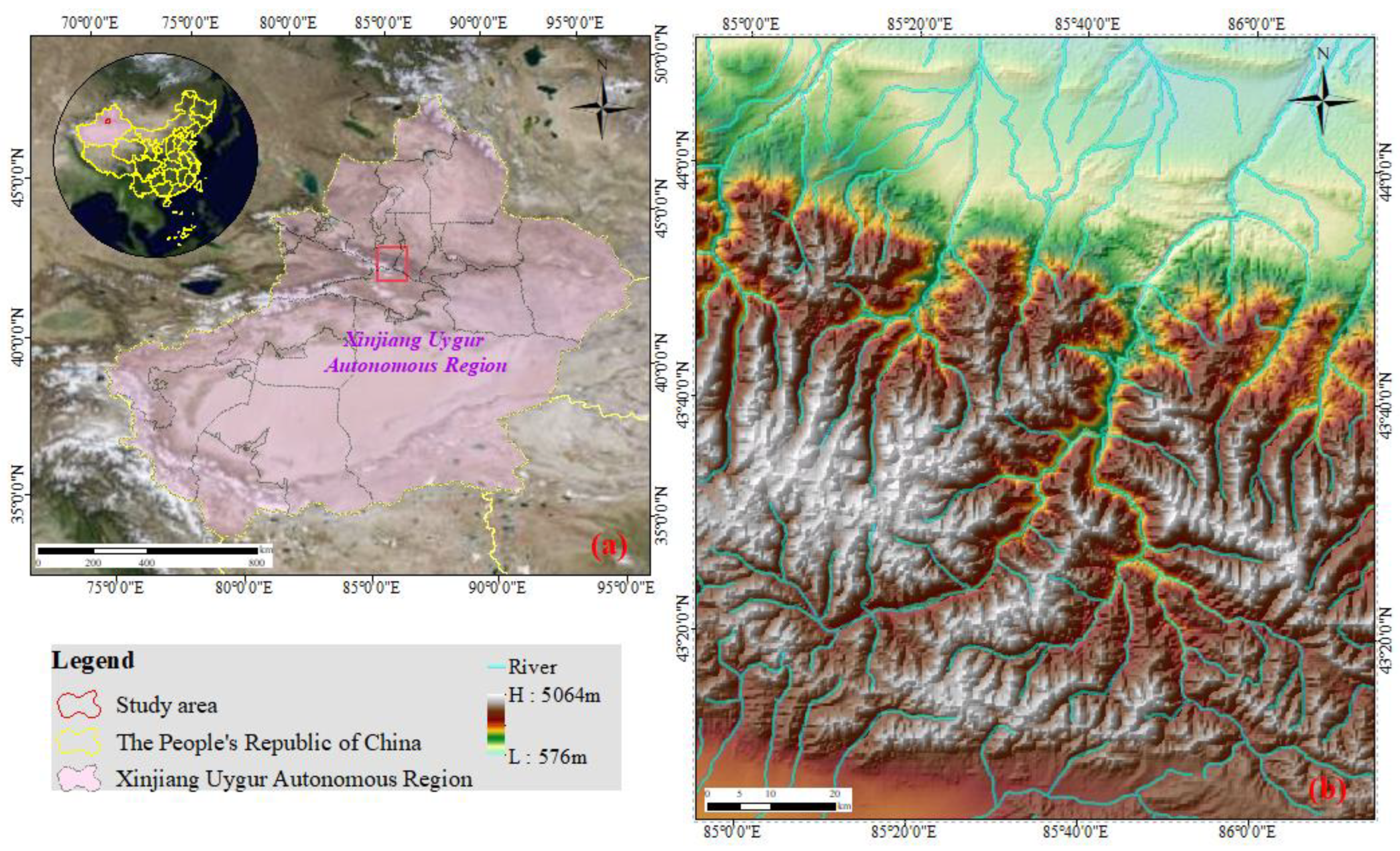
2.1. Study Area

The Manas River Basin (MRB) watershed is a subbasin of the northern Tianshan mountains in the Xinjiang Uygur autonomous regions (Figure 1). The Manas River Basin and its surrounding areas were selected as the research area, as shown in the rectangular area in Figure 1b. The areal extent lies between 84°50′E to 86°20′E longitude and 43°05′N to 44°30′N latitude, covering an area of about 5156 km². The terrain is low in the north and high in the south, and the elevation range is from 576 to 5064 m. Dominated by a typical temperate continental arid and semiarid climate, this area is characterized by extreme summer and winter temperatures [44]. The snow cover is mainly distributed in the northwestern and northern MRB. The snow cover percentage increases with elevation, from 95% in winter to 15% in summer. The snow began to accumulate in early November, and the depth reached its peak in mid-February of the following year (the snow depth in the middle of the mountains was more than 20 cm, and the snow depth in the high mountains was more than 50 cm). After that, the snow depth decreased rapidly, and the snow cover disappeared in early May. The vegetation cover is high, and the subalpine meadow zone and the mountain forest zone are distributed vertically [44]. The primary water sources for the MRB originate from snow meltwater and precipitation within the central Tianshan Mountains. The absolute maximum and minimum temperatures are 40 °C and −38 °C, respectively, with an annual average temperature of 6.2–7.8 °C. The yearly accumulated temperature over 10 °C is 2400–3500 °C.

2.2. Data Sources

Multisource remote sensing datasets were collected to extract the snow cover status and influencing factors, which were then used as independent and dependent variables in the spatial panel models.

As shown in

Table 1. The data source of snow cover metrics and influence factors.

Data Type	Data Name	Description	Abbreviations	Spatio-Temporal Resolution	Data Source	Periods
Reflectance data L-1	Landsat8 OLI/TIRS	Shady eliminated snow index	SESI	30 m/16 days	https://earthexplorer.usgs.gov/	Accessed on 15 dates as 10 and 26 February 2015, 3 and 19 March 2015, 12 and 24 April 2015, 23 March 2017, 24 April 2017, 10 May 2017, 10 and 13 March 2018, 14 April 2019, 13 and 15 March 2020, and 2 May 2020.
Meteorological variables	MOD02HKM	Land surface temperature	LST	500 m/Daily	https://modsi.gsfc.nasa.gov/
	China meteorological forcing dataset	Ai temperature	TEMP	5 km/Daily	https://data.tpdc.ac.cn/zh-hans/data/8028b944-daaa-4511-8769-965612652c49
		Wind speed	WSP
		Solar radiation	SRAD
		Precipitation	PRCP
Terrain parameters	GDEM v2	Elevation	ELE	30 m/-	https://www.gscloud.cn/sources/accessdata/421?pid=302
		Slope	SLP
		Aspect	ASP
		Roughness	ROUG
Hydrological parameters	Distribution data of lakes and rivers in Xinjiang	Distance from the river	RDIS	1:250,000 Vector data/Annual	http://www.ncdc.ac.cn/portal/metadata/d9c87a38-cdec-43f6-9c8c-f6ce82a8bce4

, descriptions of the detailed information and data sources of the dataset are listed. For the snow cover information, we collected the cloud-free optical reflectance data of Landsat 8-OLS/TIRS from February to May in the years 2015–2020. The influencing factors dataset comprised the following: (i) meteorological variables, including land surface temperature (LST), air temperature (TEMP), solar radiation (SRAD), vegetation data (NDVI), wind speed (WSP), and precipitation (PRCP). LST was inversed from Landsat 8-TIRS data and atmospheric water vapor data from MOD02HKM. The vegetation variable was calculated with the normalized difference vegetation index from Landsat 8 data. The other meteorological variables were extracted from the China meteorological forcing dataset (CMFD); (ii) terrain parameters, such as elevation (ELE), slope (SLP), aspect (ASP), and terrain roughness (ROUG), were calculated and resampled using digital elevation model data of GDEM version 2 with a 30 m resolution. Among them, the terrain roughness characterizes the variability or irregularity in elevation within a spatial unit; (iii) hydrological parameters, including the vector distribution map of lakes and rivers, were obtained from the distribution dataset of 1:250,000 lakes and rivers in Xinjiang, which was extracted from Landsat-TM data. This hydrological parameter of the river network was calculated to extract the distance from the river (RDIS).

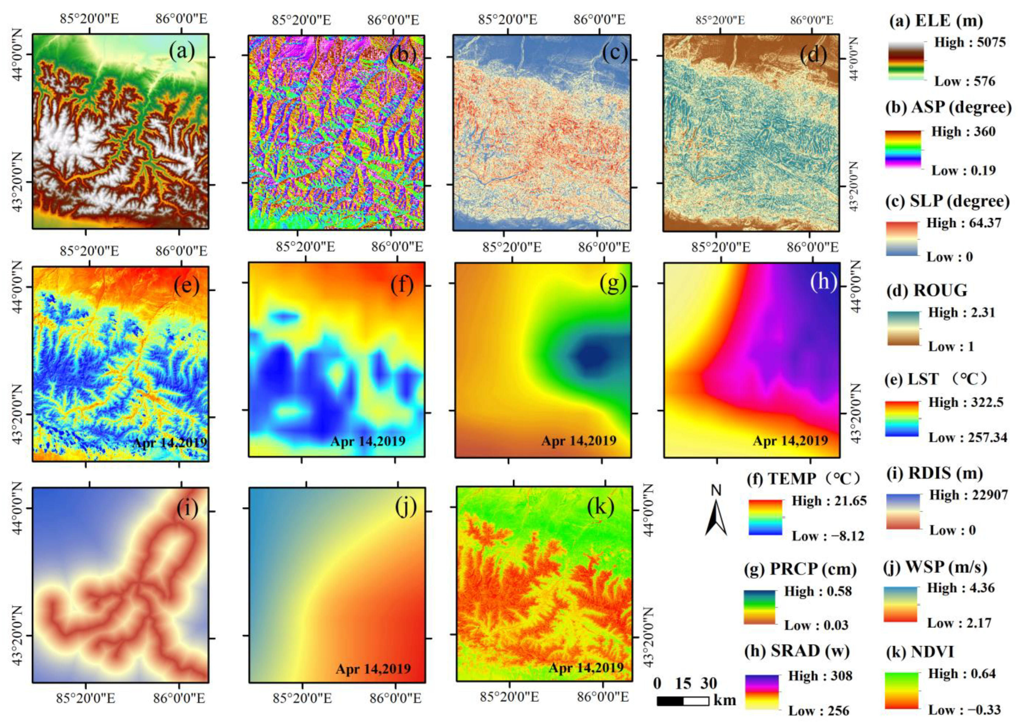
2.3. Integration of the Influencing Factors

Figure 2 is an integrated map of the eleven multisource influencing factors using a specific date as an example. Table 1 lists the selected influencing factors along with their abbreviations and descriptions. Considering the different sources and spatial resolutions of CMFD, we applied the downscaling model and resampling techniques to produce a consistent dataset with the Landsat instruments for further applications.

Specifically, given the scarcity of meteorological station data in the study area, we employed a random forest downscaling algorithm to scale down the 5 km CMFD data to 500 m using data from meteorological stations, the 500 m resolution DEM, NDVI, latitude, and surface temperature obtained from Xinjiang, China. Subsequently, the aforementioned meteorological variables and parameters were resampled to 30 m. Furthermore, compared with the daily precipitation rate, the cumulative effect of multiday precipitation on the snow melting process is more prominent. The cumulative precipitation is calculated by adding the daily precipitation between two consecutive periods. In this study, we used multiday cumulative PRCP instead of daily PRCP to comprehensively and accurately measure the effect of rainfall on snow cover change.

3. Methodologies

3.1. Overall Methodology

For data preparation, we first applied an algorithm called the shady eliminated snow index (SESI), which we established in our previous work [45]. This algorithm can effectively reflect changes in both the area covered by snow and the status of snow cover, distinguishing between new snow and old snow. Based on this algorithm, we used cloud-free Landsat 8-OLS/TIRS optical remote sensing data to extract multiple periods of snow cover status indices, which were then used as dependent variables in the “snow-factor” spatial panel model. We also included multiple influencing factors as independent variables in the spatial panel model.

An approach was established as follows. First, to distinguish the spatial pattern of snow influence factors, three spatial panel models were applied to analyze the correlation between multiple impact factors and SESIs. The fitting results under different panel models and neighboring spaces were compared to determine the influence pattern of the factors. Subsequently, the panel model with the optimal goodness of fit was selected, and impact factor assessments were conducted continuously on the continuum scale. Variation characteristics of key influencing factors were analyzed across different scales. Finally, we constructed an optimal spatial scale definition method and quantitatively measured the key influencing factors within the subbasin.

3.2. Snow Cover Index Calculations

The variation in the snow cover status is manifested not only through changes in its range but also through changes in its condition on the surface of the snowpack. These latter changes are particularly significant during the early stages of the melting period. Therefore, to comprehensively extract the snow cover status, we employed the concept of snow aging from our previous study [45]. Previous research has shown that the aging process of snow is typically observed through an increase in grain size under microscopic examination. The snow grain size index (SGI) has been widely used to differentiate between snow and non-snow pixels and indicates the extent of grain size increase using green and shortwave infrared bands [46]. The principle behind using the SGI to assess the age of snow is that within the wavelength range from 350 to 1050 nm, as the grain size increases, the reflectance typically demonstrates a decreasing trend. By normalizing the reflectance in the green and shortwave infrared bands, we can establish a distribution of SGI values that reflect changes in the size of snow grains. The index introduced in this study is a shadow-eliminated snow index (SESI) that can minimize misidentification of snow cover status caused by variations in incident angle and mountainous terrain. By incorporating the shadow-adjusted index and SGI, we can use optical remote sensing data to represent different states of snow, such as new snow, melting snow, and old snow that has melted away. The higher the index value, the newer the snow state, i.e., the state where the melting has not yet begun. Conversely, the lower the index value, the older the snow state, i.e., the snow is in the tail end of melting.

To calculate the SESI, the specific steps were as follows: The optical remote sensing image was preprocessed sequentially through sensor calibration, orthorectification, atmospheric FLAASH, and terrain correction of SCS + C. The optimization effect of preprocessing on the reflectivity of shadow areas is evaluated by analyzing the correlation between the pixel value of the remote sensing image and the cosine value of the sun’s effective incidence angle. The calculation formula for the $SESI$ is as follows:

$$SESI=SGI+c\times \frac{R_{max}-R}{R}$$

(1)

• $SGI$ is the value that normalizes the reflectance in the green and shortwave infrared bands [46], $R$ represents the reflectance of the red band, $R_{max}$ represents the maximum reflectance of the red band, and $c$ is the shadow regulator. The optimum matching algorithm is used to determine the value of shadow adjusting factor $c$. First, select the terrain effect prominent area, the initial value of a given $c$ equals 0 and 0.001 as a step for circulation, until the shadow area and highlight areas of snow index value equal or similar (the general difference is less than 0.01) end loop adjustment factor $c$ value.

3.3. Spatial Panel Regression (SPR) Modelling and Evaluation

The spatial panel regression model is a classic model in the field of spatial economics that can reflect the interactive effects and spatial spillover effects between geographical units [47,48]. The spatial panels refer to georeferenced point data over time or to spatial units such as counties and regions. The definition of spillover effects is that changes in one region will have an impact on other regions, and the dependence structure between different geographical units is related to location and distance to some extent [49]. We believe that the spillover effect in spatial interaction is very consistent with the characteristics of the snow melting process, i.e., there is an interaction between the snow state of one region and that of neighboring regions. Therefore, it is of great significance to test whether there is a statistically significant spatial spillover effect between snow state and influencing factors and quantify the scale and spatial scope of these spillover effects.

The spatial lag model (SLM), spatial error model (SEM), and spatial Durbin model (SDM) are representative models in the spatial panel regression model category. Among them, the SLM model considers the spatial spillover effect of the dependent variable (i.e., the influencing factors). The SEM discovers the effects of the omitted variables on the observation of the dependent variables, which contains a spatial error term. The SDM takes into account the spatial correlation between snow cover and adjacent areas, the spatial linear correlation between snow cover and influencing factors, and the correlation between snow cover and influencing factors in adjacent areas [50]. All of these relationships also consider spatial lag and error effects.

Considering the spatial autocorrelation and proximity effect of the snow melting process, the influence mechanism was estimated using these three candidate panel models [51]. Among them, the optimal spatial panel model was selected based on the fitting effect within these candidate models for further analysis of the multiscale effects.

Specifically, the SLM hypothesizes that the adjacent snow cover status may partially influence the snow cover of a specific location using the following formula:

$$Y_{it}=\rho {{\displaystyle \sum }}_{i=1}^N{W}_{ij}{Y}_{jt}+\beta X_{it}+{\mu }_i+{\epsilon }_{it}$$

(2)

where $Y_{it}$ is the SESI in region $i$ at time $t$ (i = 1, 2, …, N; t = 1, 2, …, t) and $W_{ij}$ is the spatial weighting matrix. Regarding the geographical effects of snow melting, the inverse distance matrix and queen neighborhood matrix (Figure A1) were adopted as the spatial weighting matrix (please refer to Appendix A for details). $\rho$ represents the spatial autoregressive coefficient, $X_{it}$ is the independent variable in region i at time $t$, $\beta$ denotes a vector of coefficients of $X_{it}$, and ${\epsilon }_{it}$ indicates the error vector.

The SEM considers the interaction effects of snow cover from both local and adjacent regions caused by omitted variables using the following formulas:

$$Y_{it}=\beta X_{it}+{\mu }_i+{\phi }_{it}$$

(3)

$${\phi }_{it}=\lambda {{\displaystyle \sum }}_{j=1}^N{W}_{ij}{\phi }_{it}+{\epsilon }_{it}$$

(4)

where ${\phi }_{it}$ is the spatially autocorrelated error term, and $\lambda$ indicates the spatial autocorrelation coefficient of the error term.

The SDM [13] considers the spatially lagged effects of both the influencing factors and the SESI using the following formula:

$$Y_{it}=\rho {{\displaystyle \sum }}_{i=1}^N{W}_{ij}{Y}_{jt}+\beta X_{it}+\gamma {{\displaystyle \sum }}_{j=1}^N{W}_{ij}{X}_{jt}+{\mu }_i+{\epsilon }_{it}$$

(5)

where $\gamma$ is the spatially autocorrelated coefficient of the independent variable, and the other variables are the same as those in the formulae mentioned above.

In this study, the dependent variable SESI has a significant spatiotemporal aggregation feature, which violates the assumptions of parameter estimation of the panel data model. The maximum likelihood estimation method is used to estimate the model parameters [52,53,54]. The classical Hausman test is used to determine whether the spatial panel data model is a fixed-effects model or a random-effects model.

The statistical testing criteria, such as the sum of squared errors, R-squared, the maximum likelihood value, Akaike’s information criterion ($AIC$), and the Schwarz criterion ($S.C.$), are jointly used to evaluate these panel autoregression models. The general forms of $AIC$ and $S.C.$ are as follows:

$$AIC=-2L/T+2K/T$$

(6)

$$S.C.=-2L/T+Klog\left(T\right)/T$$

(7)

where $K$ is the number of variables to be estimated, $L$ is the likelihood function value, and $T$ represents the number of observations.

The results of the coefficients and the statistical criteria of the spatial panel regression model are used to analyze the differences in the impact of various factors in varied adjacent intervals and to explore the influencing mechanism. The assessment was conducted by analyzing a data panel covering multiple factors and extracting the SESIs over five years.

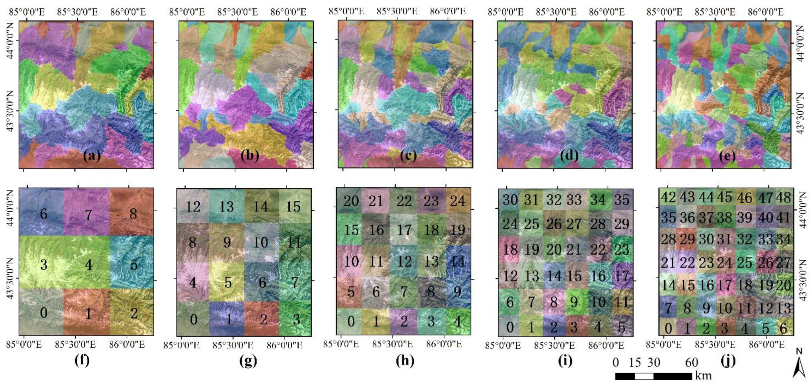
3.4. Multiscale Partitioning Scheme and Zonal Spatial Panel Model

We selected two partition schemes to divide the study area into zones of different scales. The first partition scheme involves dividing the study area into multiscale sub-catchments using the hydrological analysis tools in ArcGIS. The partition zones were extracted by filling depressions in a digital elevation model (DEM) surface raster, creating a raster of routing, simulating runoff, and calculating river network density. By referring to the small watershed division and coding specification [55], we selected threshold values of 90,000, 70,000, 50,000, 40,000, and 30,000, respectively, for river network density calculation. These threshold values correspond to the number of sub-catchments of 10, 18, 25, 36, and 50, respectively. The study area is divided on a watershed scale, considering that snow cover is an important component of the world’s water towers, and the supply and demand of water resources are interconnected on a watershed scale, with the watershed being the foundation of the water tower unit [56]. Another partition scheme divides the entire study area into grid squares, each representing a subarea. Using the fishnet creation tool in ArcGIS software, square arrays of 3 × 3, 4 × 4, 5 × 5, 6 × 6, and 7 × 7 were created based on the image of the study area. Figure 3a–j demonstrate the distribution of multiscale catchments and gridded partitions.

Further considering the multiscale effects, a separate panel model (the optimal one selected in the previous section) is applied pixel by pixel on every zone of a single scale. All panel model simulation results of each pixel in the sub-watershed were averaged to represent the characteristics of the impact factors in the subarea. We refer to the set of all models in this scale as the zonal spatial panel model. The overall fitting effect of a zonal spatial panel model is the average of all its sub-models. The significance of each influencing factor is calculated in the same manner. The characteristics of the influencing factors at different scales can be extracted from the zonal model for the corresponding scale, which is used to analyze the influence mechanism under continuous multiscales.

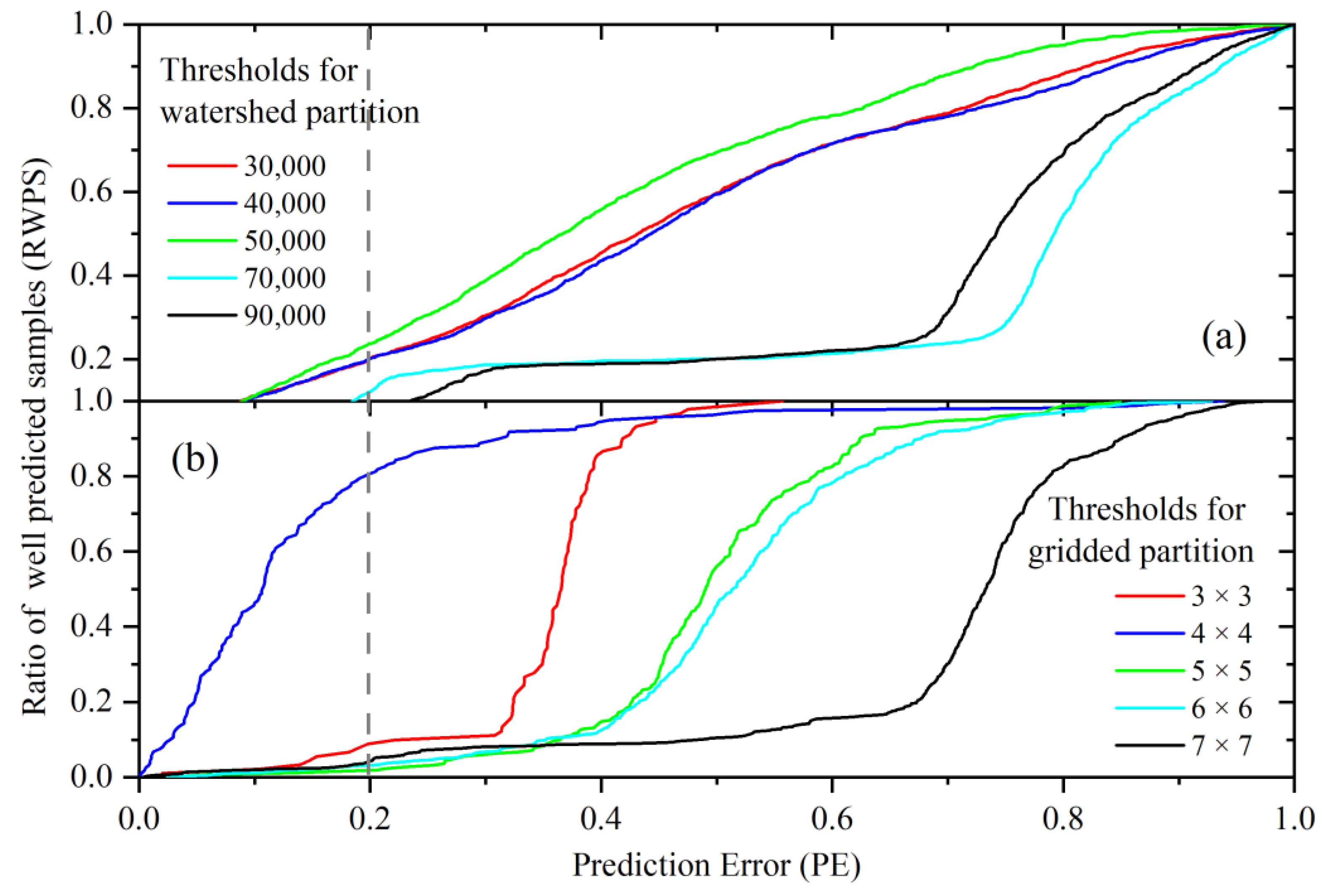
3.5. Determination and Evaluation of Optimal Partition Zone

Affected by multiple influencing factors, the snow melting process exhibits distinct characteristics within scale ranges. It is crucial to investigate the existence of an optimal partition zone and explain the snow melting process in this subregion through several key influencing factors. This so-called optimal partition zone refers to the same or similar values of SESI or the relationships of influencing factors in a specific area or the same or similar spatial phenomena.

An alternative empirical evaluation method proposed by Gao [57] was used to determine and evaluate the optimal partition zone across scales. The core idea of this empirical evaluation method is to construct a prediction rate curve to examine the comprehensive performance of the models. Samples with prediction errors falling below a specific threshold are defined as “well-predicted” samples. The prediction error (P.E.) is the difference between the estimated and observed values. We can evaluate models using the ratio of the well-predicted samples (RWPS) to the P.E., which is referred to as the “prediction rate”. Then, plot the addictive rate of n samples against the sorted P.E. The prediction rate curve of the model is obtained by joining those points. The RWPS can be indicated by the vertical axis, with P.E. being the horizontal axis. The area between the prediction rate curve and the vertical axis represents the aggregation of prediction errors. In general, a model can be considered good if this area is small. Here, we take a P.E. of less than 20% as the criterion to determine the optimal zoning scale.

4. Results

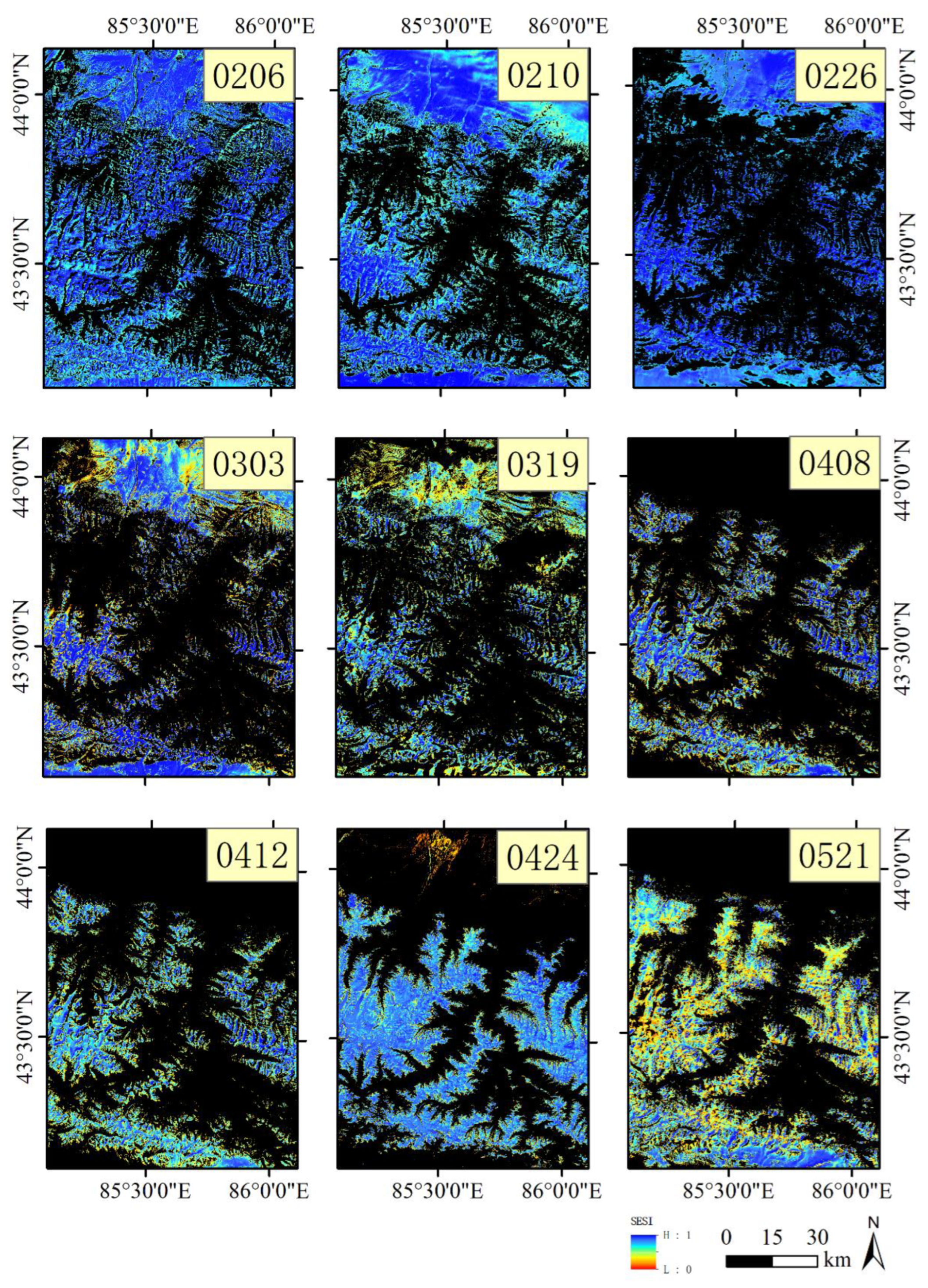
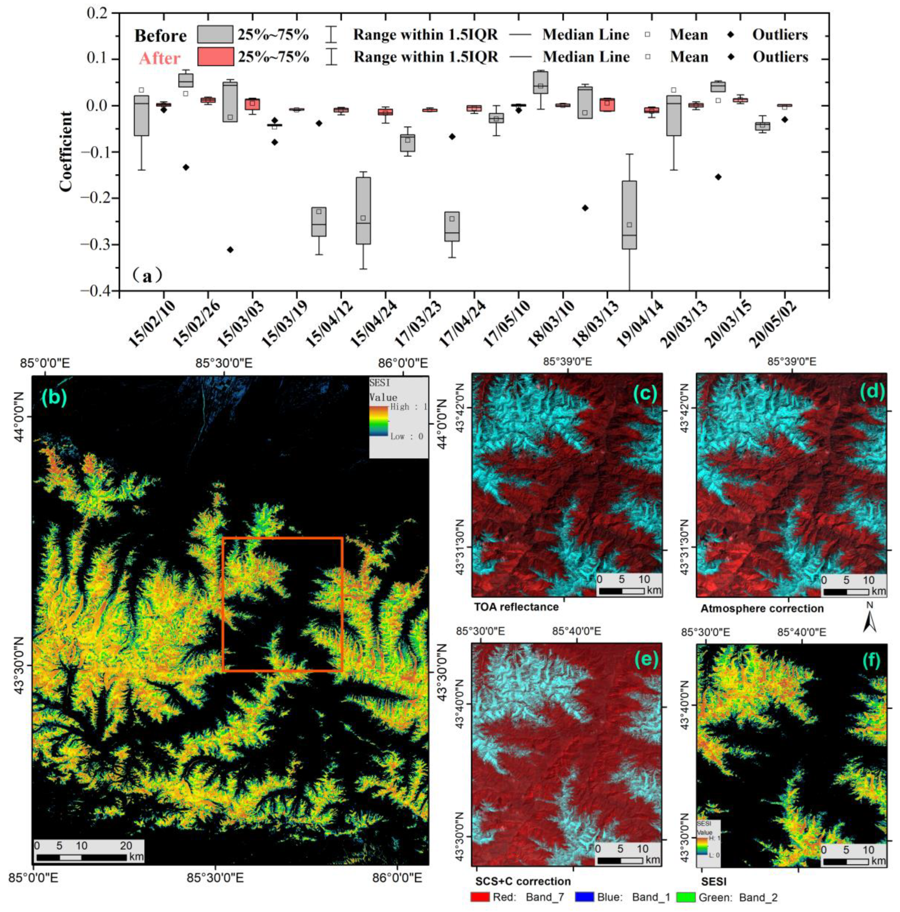
4.1. Results of Extracted SESI during the Snow Melting Period

Using the available Landsat 8-OLS data from 2015 to 2020 (Feb–May) within the MNS, fifteen periods of SESI were extracted, which depicted the typical spatial distribution of snow melting status. Figure 4a compares the coefficients for reflectance and cosine of the local incidence angle before and after preprocessing. After correction, the correlation coefficients became more stable and were closer to zero, with no more extreme values, and the difference between the upper and lower quartiles significantly decreased. Figure 4b shows the spatial distribution of the extracted SESI on 14 April 2019. The stepwise results, including the TOA reflectance, reflectance after atmospheric correction, reflectance after SCS + C terrain correction, and extracted SESI, are displayed as partially enlarged false-color images in Figure 4c–f, respectively. The multiphase SESI was extracted using the above method. The spatial distribution map of snow SESI (Figure A2) during the ablation period and the corresponding spatiotemporal variation analysis are described in Appendix B (please refer to Appendix B for details).

4.2. Mechanism of Spatial and Proximity Effect of Snow Influence Factors

Based on the Hausman tests, the p-values were significant at the 1% level; therefore, we chose the fixed-effect model to analyze the influencing factors of snow melting. As shown in Figure 5a, the regression coefficient of the 11 factors of the SLM, SEM, and SDM models with the queen and IDW proximity matrices were graphed. The R², AIC, S.C., and logarithmic likelihood values of the SLM, SEM, and SDM models were graphed in Figure 5b.

As shown in Figure 5a, through the positive and negative nature of the correlation coefficients, it is possible to determine whether the influencing factors promote or slow down snow melting. In the three panel models, the following commonalities were found: An increase in LST, TEMP, and RDIS results in intensified snow melting. The rise in ELE, NDVI, and ROUG causes a deceleration of snow aging. The correlation coefficients of the other influencing factors were all positive values close to zero, indicating that an increase in their values had an overall promoting effect on snowmelt, but the effect was weak. Relatively, the absolute values of the correlation coefficients of each influence factor in the SDM model were the highest among the three models.

The significance and magnitude of the factors differ across the panel models. In the SLM model, only one factor (ELE) achieved a significance level of 0.1%, three factors (LST, NDVI, TEMP) had a significance level of 1%, and two factors (ASP, PRCP) failed to reach a significance level of 10%. In the SEM model, two factors (ELE and TEMP) achieved a significance level of 0.1%, whereas five factors (LST, ROUG, NDVI, and SLP) had a significance level of 1%. Under the SDM model, three factors (ELE, NDVI, and TEMP) had a confidence level exceeding 0.1%. LST and ROUG were significant at the 1% level. Overall, ELE, LST, NDVI, and TEMP were highly significant across all three models. Comparatively, the SDM model had the highest number of significant factors and the highest level of significance. This indicates that the spatial lag effect between the influencing factors and snow melting is significant.

Based on the SDM model, the ROUG, TEMP, ASP, and RDIS factors exhibit slightly stronger significance than those in the SLM and SEM models. This suggests that these factors have a stronger spatial proximity effect on snowmelt. On a watershed scale, the order of factors with strong spatial proximity effects is LST, ELE, SLP, NDVI, and TEMP. However, the WSP, SRAD, and PRCP factors based on the SDM model do not exhibit greater significance than those in the SLM and SEM models. This indicates that these factors may not have a significant spatial proximity effect on snowmelt on a global scale. By comparing the modeling effects of impact factors based on the SDM model under the IDW and queen adjacency matrices, we can generally distinguish the extent of spatial proximity effects of different impact factors. The results reveal that the correlation coefficients of LST, ELE, ROUG, NDVI, and SLP based on the IDW adjacency matrix are slightly higher than those found on the queen adjacency matrix. This suggests that the spatial proximity effects of the aforementioned five impact factors are more significant beyond the pixel scale rather than only within neighboring pixels.

As shown in Figure 5b–e, on a global scale, the significance levels of the three models vary. The overall characteristics are as follows: among the three panel models, the R²(coefficient of determination) and logarithmic likelihood values of the SDM model are the highest, followed by the SEM and SLM models. The Akaike information criterion (AIC) and Schwarz criterion (S.C.) values are lowest for the SDM model, followed by the SEM and SLM models. In addition, there is a slight difference between the significance of three panel models under the two adjacency matrix models. Of the three models, the S.C. and logarithmic likelihood values of panel models with IDW adjacency matrix are all slightly lower than those with the queen adjacency matrix.

In summary, during the process of snow melting, specific factors can either accelerate or retard the rate of melting. The complexity of the melting process is attributed to the variable number and significance of local key factors, as well as the diverse range and degree of influence of neighboring factors. The melting of snow is influenced by a multitude of factors within the region, snow conditions in neighboring areas, and the combined effect of neighboring influencing factors.

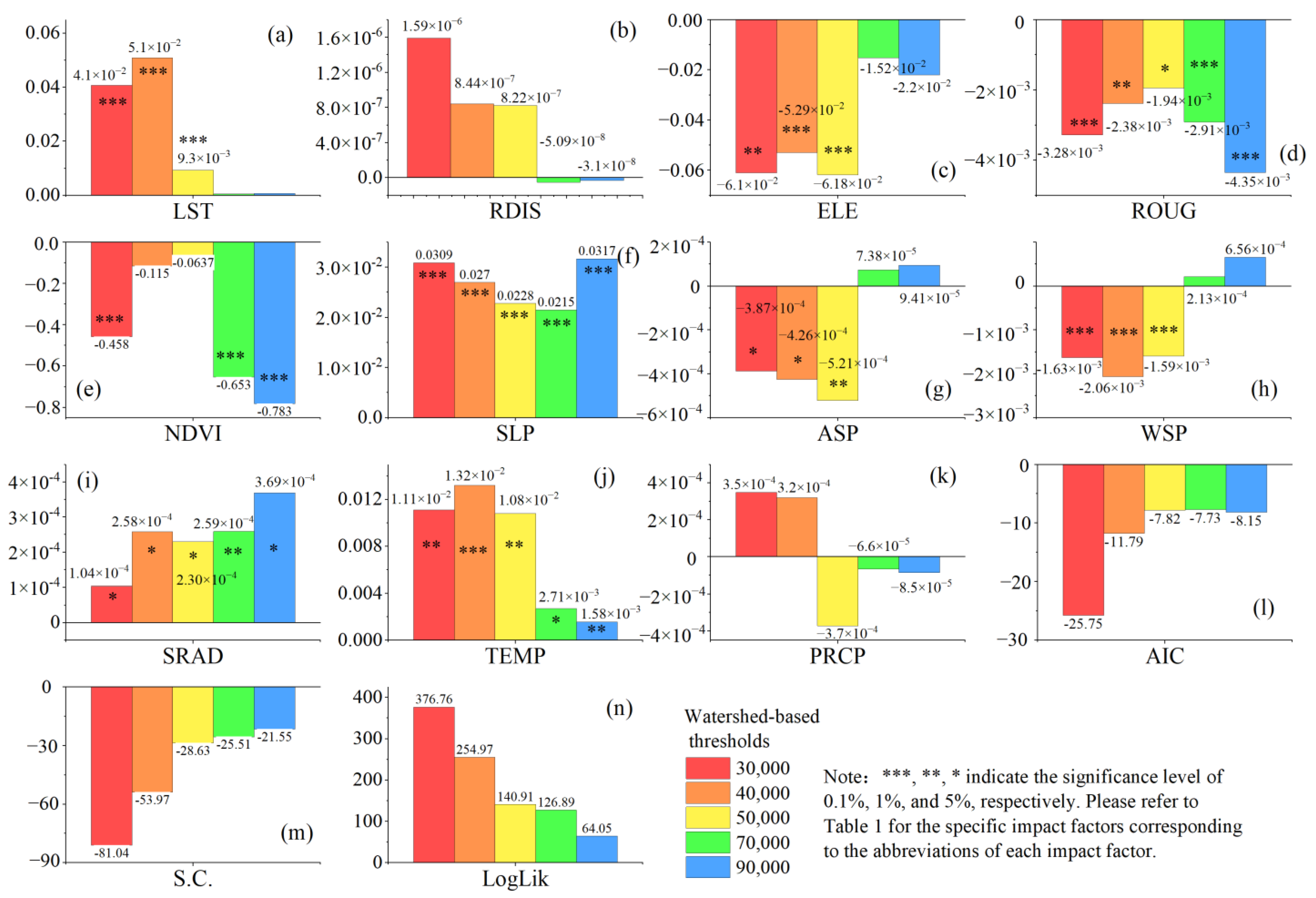
4.3. Characteristics of Influence Factors under Multiple Scales

The significance level of the influencing factors varies across scales. The simulated SDM model has the highest R², lowest AIC, he highest S.C., and highest log-likelihood values of all three models. The SDM model has a more powerful explanatory ability and better fits the snow melting process studied here. Therefore, it is selected as the optimal panel model for building zonal panel models to judge the prominent influencing factors under the two partitioning schemes at different scales.

Figure 6 presents the overall regression results and the significance of the influencing factors under watershed partitions. The significance and correlation coefficients of the influencing factors vary across different scales of watersheds, but their variation ranges are still on the same order of magnitude. Influencing factors such as LST, ELE, NDVI, SLP, TEMP, and ROUG were more significant at different size scales of watersheds, whereas RDIS and PRCP are not significant at all scales of watersheds. As the watershed-based scale decreases from large to small, the correlation coefficient and significance of specific factors show a trend of first increasing and then decreasing, such as LST, ELE, ASP, and WSP. It is worth noting that the significance of the factors changes significantly at scales exceeding a certain threshold. For example, in watersheds larger than the threshold of 50,000, the correlations of factors such as LST, ELE, WSP, TEMP, and RDIS are significantly higher. In watersheds smaller than the threshold of 70,000, the significance of NDVI increases significantly. The positive and negative values of the correlation coefficients for certain impact factors vary with scale, such as the ASP, WSP, and PRCP correlation coefficients at a watershed scale of less than 70,000, which tend to be closer to the negative value of zero. This indicates that the above factors are more significant at a watershed scale greater than the threshold value of 70,000, whereas at a watershed scale less than the threshold value of 70,000, the change in the significance of the positive and negative values may be due to estimation errors.

Figure 7 presents the overall regression results and the significance of the influencing factors under gridding partitions. The significance and magnitude of changes in various influencing factors within different gridding scales are similar to those based on watershed division. As the gridding-based scale decreases from large to small, the correlation coefficient and significance of specific factors show a decreasing trend, such as LST, ELE, and NDVI, whereas factors such as RDIS, ROUG, SLP, and SRAD show a trend of first increasing and then decreasing. It is worth noting that the significance of the factors changes remarkably at scales exceeding a certain gridding threshold. For example, in scales larger than the gridding threshold of 5 × 5, the correlation of factors such as LST, RDIS, ELE, and WSP are significantly higher. At grid scales larger than 4 × 4, the significance of LST is more prominent, whereas at smaller grid scales, its importance decreases significantly. At a grid scale of 3 × 3, the significance of elevation becomes more significant. ASP and WSP, on the other hand, have a significant increase in importance at grid scales smaller than the gridding threshold of 6 × 6.

The above results indicate that partitioning schemes can significantly affect the significance of influencing factors at each partition level. For the grid-based partition scheme, the number of variables passing the significance test increased slightly initially and then decreased as the grid became small. For the watershed-based partition scheme, the number of variables passing the significance test decreases gradually as the watershed threshold increases. There are some commonalities between the results obtained under the two partitioning schemes. The number of highly significant influencing factors decreases with decreasing scale, whereas the significance of ELE and LST decreases as the scale becomes finer. Meanwhile, the significance of NDVI, ROUG, and SLP increases as the scale decreases. It can be inferred that, at larger scales, factors such as LST, WSP, TEMP, and ELE have stronger spatial heterogeneity than those at smaller scales, which may result in their prominent significance at larger scales. At specific larger scales, the significance of LST, ELE, and TEMP significantly increased. Because these factors are the most prominent in terms of significance, they should be particularly emphasized when simulating snow conditions at larger scales. The NDVI, ROUG, and SLP may have stronger spatial heterogeneity at specific smaller scales, resulting in their prominent significance and importance at smaller scales.

4.4. Spatial Heterogeneity of Each Influencing Factor Based on Optimal Partition Scale

Figure 8a,b display the prediction rate curves of the models of the two partition schemes at different scales. Figure 5a shows significant differences in the growing RWPS trend under the five watershed partition scales. When the watershed thresholds were from 30,000 to 50,000, the P.E. and RWPS showed a positive linear correlation. Under the premise of controlling P.E. to less than 20%, the best RWPS can be achieved in the watershed partition scheme when the threshold for watershed partition is 50,000. Figure 5b shows the multiscale model prediction rate curves with the gridding partition scheme. It was found that under the 4 × 4 gridding scale, the RWPS increased significantly to about 85%. This RWPS value is significantly higher than that under other gridding partition schemes.

By comparing the model prediction rate curves under the two partitioning schemes, we found that the 4 × 4 gridding partition scheme has the best model prediction effect, accounting for about 85% of the RWPS. This result is significantly better than the other thresholds of the two partition schemes. Therefore, we set the optimal zoning scale as 4 × 4 with a gridding partition scheme to simulate the snow melting process in the study area.

Figure 9 presents the significance at different levels and regression coefficients of each influence factor obtained from the zonal spatial panel model on 24 April 2019. The influencing factors such as ELE, LST, TEMP, SLP, NDVI, ROUG, RDIS, and SRAD in zones 4, 6, 7, 8, 9, 10, and 15 all passed the significance tests at various levels. Among them, the significance level of the influencing factors in zones 6, 8, 9, 10, and 15 are the same and all passed the 0.1% significance test. Other factors passed the significance test except for PRCP, WSP, and RDIS. Only one impact factor did not pass the significance test in zones 0, 1, 11, and 14. WSP did not pass the significance test in zones 1, 3, and 11, and RDIS did not pass the significance test in zone 14. ELE, NDVI, LST, ROUG, and SLP all passed the significance test in all zones. The impact of ELE had the most significant positive impact on the change in SESI. The effect of NDVI on SESI is negative. Such an effect in zone 4 is weaker than that in the rest of the zones. The SRAD had the lowest degree of impact and failed the significance test in zones 0, 2, 3, 5, 12, and 13. Generally, the significance of influencing factors on SESI is ranked as follows: ELE, NDVI, LST, ROUG, SLP, RDIS, WSP, and SRAD.

The correlation coefficients of ELE in all zones were relatively high, with an average value greater than 0.05, showing a significant negative correlation characteristic. There is a regional difference between the north and south in the correlation coefficient of LST. The overall correlation of SLP was also significant, with a high correlation of 0.06 in the midmountain zone. The rest of the regions have a low correlation of about 0.02. In general, the correlation of TEMP is inapparent. However, in areas located in the middle mountain belt region on the northern slope of the MRB, the correlation coefficient of TEMP is relatively significant, approximately 0.017. NDVI showed a negative correlation with snow melting across the basin. The correlation coefficient distribution was relatively even across subbasins, with a value of approximately −0.015. ROUG exhibits opposite correlation characteristics in different subbasins, with relatively weak negative correlations between zones 12, 13, and 6, 7 and snowmelt, no correlation in subbasins 14 and 15, and weak positive correlations of 0.004 with snowmelt in the remaining regions. SRAD has a weak positive correlation within zones 7–10 but is insignificant in other zones. The correlation coefficients between WSP and ASP in different regions have both positive and negative differences, but overall, the correlation is weak. However, the correlation coefficient of PRCP is very weak in the entire subbasin.

Figure 10a,b show a comparison of the observed and simulated results of the SESI based on the zonal SDM panel model on 24 April 2019. The R² exceeded 0.7 in 14 zones, with an average R² of 0.79. The disparity in significance among zones within the study area was prominent. The R² values of zones 0, 1, 12, 13, 14, and 15 were above 0.8, and those of zones 13, 14, and 15 were above 0.9, indicating that the zonal panel model increased the degree of data fitting. The zonal fitting effect was assessed using the mean absolute percentage error (MAPE). MAPE quantifies the proportion of the prediction error relative to the observed value of SESI. As the MAPE value decreases, it indicates a better fitting effect. The average MAPE for all 16 zones was 23.1%. Zones 12, 13, 14, and 15 showed the most minor fitting errors (around 15%). The accuracy assessment of the simulation was also estimated using the model prediction curve. The findings indicate that in zones 5 and 9, the percentage of samples with less than 20% P.E. was less than 80%. In other zones, RWPS with a P.E. of less than 20% could reach 100%, accounting for more than 81% of the study area.

5. Discussions

5.1. The Spatial and Proximity Interaction in the Snow Melting Process

The spatial and adjacent interactions between snow cover and environmental factors have been confirmed in many studies [13,58]. For example, investigations have been conducted to measure changes in snow reflectance due to the presence of other surrounding objects. Factors such as water bodies, sparse vegetation, dry and moist soil, coal, and carbon are considered crucial in determining the effect of an adjacent feature on the spectral reflectance of snow cover [13]. Increased snow cover would cause a shift toward negative adjacent interactions in tundra plant communities [59,60]. The above research demonstrates the significant impact of neighboring objects on snow reflectivity on a microscopic scale and verifies the impact of a specific neighboring object on the snow melting rate on a large scale.

To assess the spatial and proximity effect between the snow cover and influencing factors, three types of spatial panel models, the SLM, SEM, and SDM, were used to conduct the panel regression. The significance of ELE, LST, NDVI, and TEMP is particularly noteworthy in all three spatial panel models. Therefore, it can be inferred that during the process of snow melting, the spatial spillover effects of these influencing factors are significant, and the snow conditions in neighboring areas also have a significant impact on the local snow status. The optimal performance of the SDM model indicates the coexistence of both effects. The strong correlation between these factors and heat distribution, a key driver of snow recession, may explain their significance. For example, elevation has vertical temperature gradients, whereas LST and TEMP represent heat distribution [8]. Additionally, NDVI in high-altitude mountainous areas exhibits significant vertical patterns [17,18]. Therefore, factors closely related to heat distribution have higher significance among multiple influencing factors.

Furthermore, LST, ELE, SLP, NDVI, and TEMP exhibit a significant neighboring effect. The cause of the neighboring effect on snow has not been fully studied. We speculate that this may be due to the presence of forests in high-altitude mountainous areas, where solar radiation increases the temperature of tree canopies and leads to changes in the climate near the forest belt [15]. Alternatively, it may be caused by local special terrain resulting from terrain slope, which alters the distribution of radiation in the local area [61], affects the local climate environment, and creates effects such as cold-air pooling effects [62] and temperature inversions [63,64], thereby exerting a greater influence on the snow in neighboring areas.

5.2. The Differences in Dominant Factors Affecting Snow Melting at Varied Scales

Many studies have analyzed the response or correlation of snow cover to specific influencing factors at different scales [25,26,27,65], but few studies have analyzed the significant changes and trends of multiple influencing factors at continuous scales. Our research not only considers the changing trends in the significance and correlation of various influencing factors under multiscale continuous changes but also considers the impact of different zoning schemes on the significance of influencing factors.

We attempted to explore why there are differences in the degree of influencing factors under the two partition schemes. When designing the partition scheme, we simultaneously considered two partitioning methods: one based on a grid and the other based on hydrological catchments. We took into account that the supply and demand of water resources are interconnected at the catchment scale, and catchments are the basic units of water towers [57]. Therefore, we also considered a partitioning scheme based on river basins. However, from the perspective of multiscale fitting, the grid partitioning result of 4 × 4 grid size has a better fitting effect. One possible reason is that the river basins divided based on terrain data are different from those divided based on climate, even though the latter is usually based on mountain ridges. In addition, the threshold division of each scale in the hydrological analysis may not accurately capture the homogeneous areas with similar melting mechanisms.

Nevertheless, the variation of impact factors with scale under the two zoning schemes also showed similar generalities. The number of highly significant influencing factors decreases with smaller scales, whereas the significance of ELE and LST decreases at finer scales. Meanwhile, the heterogeneity of influencing factors at different scales can change their importance. Factors with stronger spatial heterogeneity at large scales may exhibit more significant importance at large scales, and vice versa. The causes of this heterogeneity can be attributed to two aspects. On the one hand, the heterogeneity of the factors themselves varies at different scales [66]. On the other hand, the spatial resolution of downscaled remote sensing data still has limitations [67]. For example, local terrain variations can cause differences in temperature, wind speed, and radiation at small scales [68,69,70], but these differences are difficult to reflect in existing meteorological driving data. The missing meteorological stations also make it difficult for downscaling algorithms to improve local accuracy [71]. Therefore, the role of meteorological factors on a small scale still needs further exploration.

5.3. Heterogeneity of Local Influencing Factors

The local heterogeneity of influencing factors has been widely studied, with a general acceptance that geographical latitude, altitude, and air temperature primarily regulate snow accumulation and ablation processes [72,73,74]. In each sub-region within our study area, both ELE and LST exhibited significant effects, but the influence of latitude was not taken into account. Other research indicates that TEMP and PRCP play a principal role in controlling the spring snow cover fraction (SCF). Such influence is particularly strong within a specific elevational range [75]. For example, in the Keriya River Basin, the influence of TEMP on SCF is concentrated within an elevation range of 5175–6425 m, whereas PRCP serves as the main controlling factor at elevations of 2475–5175 m and above 6425 m [76]. Wu et al. identified two distinct threshold elevations in the MRB. Below a threshold elevation of 3900 ± 400 m, snow cover exhibits an inverse correlation with TEMP and a positive correlation with PRCP, and vice versa above this threshold elevation [77]. Additionally, above the threshold elevation of 1400 ± 100 m, TEMP becomes the main factor [78]. Under the premise of comprehensively considering the spatial effects of multiple influencing factors, we found that the significant impact of TEMP is more prominent in the high-altitude areas of the northern slope of MNS, whereas its significance is noticeably weaker in the low-altitude areas of both the southern and northern slopes of the MRB. Our results further confirm the influence of complex climate factors, with temperature being an essential factor that affects snow cover change.

Topographic factors such as ELE, ASP, SLP, and ROUG are related to one another and act in unison to exert an overall topographic effect [72]. Regarding the relationship between ASP and snow cover, the north-facing slopes had remarkably large snow cover ratio and snow cover duration values compared with those of the south-facing slopes, corroborating previous studies that emphasized that snow accumulates most on north-facing slopes [72,73]. However, such a relationship exhibits distinct seasonal differences in that the spatial variability of the snow cover ratio with aspect is most significant during winter. This may explain why the significance of ASP was not so prominent in spring in our study.

We also found that the significance of SLP and ROUG was significant in each subregion. In zones 9, 10, and 11 on the northern windward slope, the importance of WSP was significantly higher than that on the southern leeward slope. This is not difficult to explain, as the north slope of Tianshan Mountain is affected by water vapor from both the Atlantic and Arctic oceans compared to the south slope. It can be inferred that heat input in the upper layer of snow is the main cause of snow melting, whereas terrain redistributes heat input and wind speed alters the distribution of energy. The specific terrain also changes the wind speed, which then alters the location and state of snow accumulation. Many existing research conclusions support the above statements. For example, terrain properties such as slope and aspect have been found to affect the incoming solar radiation on the surface by modifying the intensity and duration of sun exposure at a given location [77,78,79]. Due to temperature gradients [79], snow on sunward aspects is less persistent than that on shaded slopes. Windward slopes accumulate more snow than leeward slopes as moisture converges in that direction [75]. Steeper slopes tend to have less snow than flatter slopes due to gravity [77]. It should be noted that this study examines which factors have a more significant response to the process of snow melting rather than the causal relationship between the factors. Therefore, there are significant spatial and temporal heterogeneities in the significance of various factors at a local scale.

5.4. Comparison with Existing Methods

Current research on the analysis of influencing factors in the process of snow accumulation or ablation mainly relies on long-term time series of snow parameters and influencing factors. Researchers often conduct linear or nonlinear correlation analyses between independent and dependent variables to quantitatively assess the dominant influencing factors of snow’s spatial and temporal processes [31,32,33,34,35,36]. However, such studies often only consider factors such as topographic or hydrothermal elements [11,14,29]. To gain a deeper understanding of the dominant factors driving snow accumulation and ablation, some researchers have conducted long-term observations at field measurement sites, where they select relatively homogeneous snow areas and control variables to explain the changes in snow accumulation and ablation [6,13,17]. These field measurements can more accurately capture the influencing factors at the upper and lower edges of the snow cover, as well as internal changes within the snow layer. However, the regional representativeness of these findings is often limited, making it challenging to characterize the influence mechanisms of snow cover at larger scales. Some studies consider the spatial heterogeneity of snow cover, but they often use pixels as the basic analysis unit to analyze the causes of the uneven spatial and temporal distribution of snow cover in different regions (such as detecting differences in the impact factors of different altitude zones) [32,77,78,79]. Such studies also do not consider the spatial effects of snow cover impact factors.

Although these approaches provide insights into how snow cover properties relate to each of these influencing variables, sequential regression-type relationships only explain a small percentage of the variability, and no unique relationship can be defined for different environments due to differences in the dominant processes in different locations. The unique advantage of the spatial panel data model is that it can analyze multiple spatial effects between independent and dependent variables. For example, in this study, the neighborhood effect, spatial correlation, and multiscale effect can all be included in the measurement of influencing factors. Comparatively speaking, our method relies less on time series data. The panel data used for each period are relatively independent. In addition, although there are many snowmelt runoff models based on physical processes, most of these simulations are based on independent pixels to simulate and predict snowmelt, and few of them take the spatial effects of influencing factors into consideration. We believe that the above spatial effects cannot be ignored in the spatial–temporal process of snow cover. The exploration in this article is an important supplement to the spatial–temporal mechanism of snow cover.

5.5. Limitations and Perspectives

It is essential to acknowledge discrepancies in the dataset composition. In this study, the significance of PRCP was not prominent. This is likely due to the difficulty in accurately capturing precipitation events based on the downscaled precipitation data from the CMFD dataset, resulting in insufficient accuracy of the precipitation dataset and making it difficult to reflect its correlation with snow cover changes in local space-time. Solar radiation, wind speed, and other factors may also be unable to accurately capture their significance due to their low temporal and spatial accuracy. The influencing factors of the lower edge of the snow layer, such as frozen soil, soil temperature, and humidity, have not been considered in this article, but their importance cannot be ignored. In addition, temperature and solar radiation may have a time lag effect on snow melting, as the temperature may have increased for several days before melting begins. Thus, the heat accumulation effect of temperature and radiation should also be considered.

In this study, we compared the goodness-of-fit of various panel data models based on different adjacency matrices, enabling preliminary discrimination between the proximity effects of various influencing factors. It was found that LST, ELE, SLP, NDVI, and TEMP are factors with significant proximity effects that are expressed within different ranges. However, the specific roles of each influencing factor in the process of snow melting under different adjacency matrices were not distinguished. It is evident that quantitatively measuring the range and extent of the proximity effect of various influencing factors will be a meaningful task in the next step. Additionally, it is necessary to take into account the time lag effect resulting from snow cover and the influence of other factors. We suggest using a variable distance adjacency matrix for the influencing factors in the panel model and adding a time-lag variable to improve our understanding of this system.

6. Conclusions

In this study, we established a connection between snow cover characteristics and influencing factors using a zonal panel model. The results showed that multiple unequally distributed influencing factors are related to one another and act in unison to exert an overall effect on the snow melting process. A framework of the zonal spatial panel model is proposed to determine the influencing mechanism of snowmelt with respect to spatial, proximity, and heterogeneity effects. The main findings of this study are as follows:

First, there is a prominent spatial interaction and proximity effect between snow cover and the influencing factors. The spatial dependency and magnitude and extent of the proximal effects of influence factors display spatial heterogeneity. ELE, SLP, LST, and NDVI have significant correlation coefficients and significance levels that manifest as the overall dominant influencing factors for snow melting. The impact factors with distinct proximity effects on a watershed scale are ranked as follows: LST, ELE, SLP, NDVI, and TEMP.

Second, different partition schemes and scales can significantly impact the relative importance and significance rank of the dominant influencing factors within the region. The count of highly significant influencing factors decreases with decreasing scale, whereas the significance of ELE and LST decreases as the scale becomes finer. Conversely, the significance of ROUG, RDIS, and SLP increases as the scale decreases. At a specific scale, the significance of influence factors such as ELE, NDVI, and LST will change significantly. For example, at a certain larger scale, the importance of LST, ELE, and TEMP will increase significantly, whereas at a certain smaller scale, the significance of NDVI, ROUG, and SLP will increase significantly. The spatial heterogeneity of various influencing factors might be the main reason for the differences in significant factors at multiple scales.

Third, the significance of the impact factors varies significantly within each subregion. Topographic factors such as ELE, SLP, and ROUG have significant correlations throughout the basin. The significance of LST, TEMP, and WSP exhibits a north–south difference in the MNS. The significance of NDVI is relatively even across the region, whereas the overall significance of SRAD, ASP, PRCP, and RDIS is weak.

This research demonstrates that the spatial, proximity, and multiscale effects between snow cover and numerous influencing factors should be fully considered in elucidating the influencing mechanism of snow cover. When simulating the spatial and temporal variation process of snow cover at different spatial scales, a number of influencing factors should be prioritized and screened. Methodologically, establishing a zonal spatial panel analysis is possible and can effectively capture the spatial interactive impacts of multiple factors on snowmelt. Given the growing number of upcoming satellite sensors with new capabilities in frequencies, image modes, and revisit times, the panel technique may be a robust and convenient approach for investigating the effects of influencing factors.

7. Patent

Haixing Li has patent #CN 115329561B, licensed to Nanjing Tech University.

References

1. Ahluwalia, R.S.; Rai, S.P.; Meetei, P.N.; Kumar, S.; Sarangi, S.; Chauhan, P.; Karakoti, I. Spatial-diurnal variability of snow/glacier melt runoff in glacier regime river valley: Central Himalaya, India. Quat. Int. 2021, 585, 183–194. [Google Scholar] [CrossRef]
2. Guo, D.L.; Pepin, N.; Yang, K.; Sun, J.Q.; Li, D. Local changes in snow depth dominate the evolving pattern of elevation-dependent warming on the Tibetan Plateau. Sci. Bull. 2021, 66, 1146–1150. [Google Scholar] [CrossRef] [PubMed]
3. Beniston, M. Is snow in the Alps receding or disappearing? Clim. Chang. 2012, 3, 349–358. [Google Scholar] [CrossRef]
4. Matiu, M.; Crespi, A.; Bertoldi, G.; Carmagnola, C.M.; Marty, C.; Morin, S.; Schöner, W.; Berro, D.C.; Chiogna, G.; De Gregorio, L.; et al. Observed snow depth trends in the European Alps 1971 to 2019. Cryosphere Discuss. 2021, 15, 1343–1382. [Google Scholar] [CrossRef]
5. Yi, Y.; Kimball, S.J.; Rawlins, A.M.; Moghaddam, M.; Euskirchen, E.S. The role of snow cover affecting boreal-arctic soil freeze–thaw and carbon dynamics. Biogeosciences 2015, 12, 5811–5829. [Google Scholar] [CrossRef]
6. Aanderud, Z.T.; Jones, S.E.; Schoolmaster, D.R., Jr.; Fierer, N.; Lennon, J.T. Sensitivity of soil respiration and microbial communities to altered snowfall. Soil. Biol. Biochem. 2013, 57, 217–227. [Google Scholar] [CrossRef]
7. Notarnicola, C. Hotspots of snow cover changes in global mountain regions over 2000–2018. Remote Sens. Environ. 2020, 243, 111781. [Google Scholar] [CrossRef]
8. Li, H.; Liu, J.; Lei, X.; Ju, Y.; Bu, X.; Li, H. Quantitative determination of environmental factors governing the snow melting: A geodetector case study in the central Tienshan Mountains. Sci. Rep. 2022, 12, 11565. [Google Scholar] [CrossRef]
9. Schweizer, J.; Kronholm, K. Snow cover spatial variability at multiple scales: Characteristics of a layer of buried surface hoar. Cold Reg. Sci. Technol. 2007, 47, 207–223. [Google Scholar] [CrossRef]
10. Zhang, T. Influence of the seasonal snow cover on the ground thermal regime: An overview. Rev. Geophys. 2005, 43, RG4002. [Google Scholar] [CrossRef]
11. Sharma, A.; Bhattacharya, A.; Venkataraman, C. Influence of aerosol radiative effects on surface temperature and snow melt in the Himalayan region. Sci. Total Environ. 2021, 810, 151299. [Google Scholar] [CrossRef] [PubMed]
12. Burazerovic, D.; Heylen, R.; Geens, B.; Sterckx, S.; Scheunders, P. Detecting the Adjacency Effect in Hyperspectral Imagery with Spectral Unmixing Techniques. IEEE J. Sel. Top. Appl. 2013, 6, 1070–1078. [Google Scholar] [CrossRef]
13. Garg, P.K. Effect of contamination and adjacency factors on snow using spectroradiometer and hyperspectral images. In Hyperspectral Remote Sensing; Elsevier: Amsterdam, The Netherlands, 2020; pp. 167–196. [Google Scholar]
14. Roots, E.F.; Glen, J. Hydrological aspects of Alpine and high mountain areas. In Proceedings of the Exeter Symposium, Exeter, UK, 19–30 July 1982; International Association of Hydrological Sciences: Oxfordshire, UK, 1982; pp. V–VI. [Google Scholar]
15. Currier, W.R.; Lundquist, J.D. Snow depth variability at the forest edge in multiple climates in the western United States. Water Resour. Res. 2018, 54, 8756–8773. [Google Scholar] [CrossRef]
16. Andreadis, K.M.; Storck, P.; Lettenmaier, D.P. Modeling snow accumulation and ablation processes in forested environments. Water Resour. Res. 2009, 45, W05429. [Google Scholar] [CrossRef]
17. Sanmiguel-Vallelado, A.; McPhee, J.; Carreño, P.E.O.; Morán-Tejeda, E.; Camarero, J.J.; López-Moreno, J.I. Sensitivity of forest–snow interactions to climate forcing: Local variability in a Pyrenean valley. J. Hydrol. 2022, 605, 127311. [Google Scholar] [CrossRef]
18. Watson, F.G.; Anderson, T.N.; Kramer, M.; Detka, J.; Masek, T.; Cornish, S.S.; Moore, S.W. Effects of wind, terrain, and vegetation on snow pack. Terr. Ecol. 2008, 3, 67–84. [Google Scholar]
19. Verbunt, M.; Gurtz, J.; Jasper, K.; Lang, H.; Warmerdam, P.; Zappa, M. The hydrological role of snow and glaciers in alpine river basins and their distributed modeling. J. Hydrol. 2003, 282, 36–55. [Google Scholar] [CrossRef]
20. López-Moreno, J.I.; Gascoin, S.; Herrero, J.; Sproles, E.A.; Pons, M.; Alonso-González, E.; Hanich, L.; Boudhar, A.; Musselman, K.N.; Molotch, N.P.; et al. Different sensitivities of snowpacks to warming in Mediterranean climate mountain areas. Environ. Res. Lett. 2007, 12, 074660. [Google Scholar] [CrossRef]
21. Bi, Y.; Xie, H.; Huang, C.; Ke, C. Snow cover variations and controlling factors at upper Heihe River Basin, Northwestern China. Remote Sens. 2015, 7, 6741–6762. [Google Scholar] [CrossRef]
22. Mott, R.; Vionnet, V.; Grünewald, T. The Seasonal Snow Cover Dynamics: Review on Wind-Driven Coupling Processes. Front. Earth Sci. 2018, 6, 197. [Google Scholar] [CrossRef]
23. Walker, D.A.; Billings, W.D.; Molenaar, J.G.D. Snow-vegetation interactions in tundra environments. Snow Ecol. 2001, 20, 207–223. [Google Scholar]
24. Dankers, R.; Christensen, O.B. Climate change impact on snow coverage, evaporation and river discharge in the Sub-Arctic Tana Basin, Northern Fennoscandia. Clim. Chang. 2005, 69, 367–392. [Google Scholar] [CrossRef]
25. Han, S.Z. Linkage of the preceding winter mid-latitude Eurasian atmospheric circulation with the spring northern East Asian snow cover. Atmos. Res. 2023, 293, 106926. [Google Scholar] [CrossRef]
26. Han, S.Z.; Ren, H.L.; Su, B.H.; Li, J.X. Connection between the North Atlantic Sea surface temperature and the late autumn snow cover anomalies over the central Tibetan Plateau. Atmos. Res. 2022, 279, 106926. [Google Scholar] [CrossRef]
27. Tang, Z.G.; Deng, G.; Hu, G.J.; Zhang, H.B.; Pan, H.Z.; Sang, G.Q. Satellite observed spatiotemporal variability of snow cover and snow phenology over high mountain Asia from 2002 to 2021. J. Hydrol. 2022, 613, 128438. [Google Scholar] [CrossRef]
28. Strom, J.; Svensson, J.; Moosmuller, H.; Meinander, O.; Virkkula, A.; Hyvarinen, A.; Asmi, E. Snow cover duration in northern Finland and the influence of key variables through a conceptual framework based on observed variations in snow depth. Sci. Total Environ. 2023, 903, 166333. [Google Scholar] [CrossRef] [PubMed]
29. Mankin, J.S.; Diffenbaugh, N.S. Influence of temperature and precipitation variability on near-term snow trends. Clim. Dyn. 2015, 45, 1099–1116. [Google Scholar] [CrossRef]
30. Valt, M.; Guyennon, N.; Salerno, F.; Petrangeli, A.B.; Salvatori, R.; Cianfarra, P.; Romano, E. Predicting new snow density in the Italian Alps: A variability analysis based on 10 years of measurements. Hydrol. Process. 2018, 32, 3174–3187. [Google Scholar] [CrossRef]
31. Roh, H.-J.; Sahu, P.K.; Sharma, S.; Datla, S.; Mehran, B. Statistical investigations of snowfall and temperature interaction with passenger car and truck traffic on primary highways in Canada. J. Cold Reg. End. 2016, 30, 04015006. [Google Scholar] [CrossRef]
32. Dedieu, J.P.; Lessard-Fontaine, A.; Ravazzani, G.; Cremonese, E.; Shalpykova, G.; Beniston, M. Shifting mountain snow patterns in a changing climate from remote sensing retrieval. Sci. Total Environ. 2014, 493, 1267–1279. [Google Scholar] [CrossRef]
33. Qin, D.H.; Liu, S.Y.; Li, P.J. Snow cover distribution, variability, and response to climate change in western China. J. Clim. 2006, 19, 1820–1833. [Google Scholar]
34. Jost, G.; Weiler, M.; Gluns, D.R.; Alila, Y. The influence of forest and topography on snow accumulation and melt at the watershed-scale. J. Hydrol. 2007, 347, 101–115. [Google Scholar] [CrossRef]
35. López-Moreno, J.; Fassnacht, S.; Heath, J.; Musselman, K.; Revuelto, J.; Latron, J.; Morán-Tejeda, E.; Jonas, T. Small scale spatial variability of snow density and depth over complex alpine terrain: Implications for estimating snow water equivalent. Adv. Water Resour. 2013, 55, 40–52. [Google Scholar] [CrossRef]
36. Nicholls, N. Climate variability, climate change and the Australian snow season. Aust. Meteorol. Mag. 2005, 54, 177–185. [Google Scholar]
37. LeSage, J.; Pace, R.K. Introduction to Spatial Econometrics; Chapman and Hall/CRC: Boca Raton, FL, USA, 2009. [Google Scholar]
38. Elhorst, J.P. Serial and spatial error correlation. Econ. Lett. 2008, 100, 422–424. [Google Scholar] [CrossRef]
39. De Blas, C.S.; Valcarce-Diñeiro, R.; Sipols, A.E.; Martín, N.S.; Arias-Pérez, B.; Santos-Martín, M.T. Prediction of crop biophysical variables with panel data techniques and radar remote sensing imagery. Biosyst. Eng. 2021, 205, 76–92. [Google Scholar] [CrossRef]
40. Li, C.; Managi, S.; Wang, M.H. Estimating monthly global ground-level NO2 concentrations using geographically weighted panel regression. Remote Sens. Environ. 2022, 280, 113152. [Google Scholar] [CrossRef]
41. Fu, M.; Kelly, A.; Clinch, J.P. Prediction of PM2.5 daily concentrations for grid points throughout a vast area using remote sensing data and an improved dynamic spatial panel model. Atmos. Environ. 2020, 237, 117667. [Google Scholar] [CrossRef]
42. Hu, B.D.; McAleer, M. Estimation of Chinese agricultural production efficiencies with panel data. Math. Comput. Simulat. 2005, 68, 475–484. [Google Scholar] [CrossRef]
43. Jiang, C.; Zhao, L.; Dai, J.; Liu, H.; Li, Z.; Wang, X.; Yang, Z.; Zhang, H.; Wen, M.; Wang, J. Examining the soil erosion responses to ecological restoration programs and landscape drivers: A spatial econometric perspective. J. Arid. Environ. 2020, 183, 104255. [Google Scholar] [CrossRef]
44. Hu, R.Y. The Natural Geography of Tianshan Mountain in China; China Environmental Science Press: Beijing, China, 2004. [Google Scholar]
45. Li, H.; Liu, J.; Bu, X.; Feng, X.; Xiao, P. An Integrated Shadow-Adjusted Snow-Aging Index for Alpine Regions. Remote Sens. 2020, 12, 1249. [Google Scholar] [CrossRef]
46. Negi, H.S.; Singh, S.K.; Kulkarni, A.V.; Semwal, B.S. Field-based spectral reflectance measurements of seasonal snow cover in the Indian Himalaya. Int. J. Remote Sens. 2010, 31, 2393–2417. [Google Scholar] [CrossRef]
47. Elhorst, J.P. Spatial Panel Data Analysis. Encycl. GIS 2017, 2, 2050–2058. [Google Scholar]
48. Elhorst, J.P. Spatial panel models and common factors. In Handbook of Regional Science; Springer: Berlin/Heidelberg, Germany, 2021; pp. 2141–2159. [Google Scholar]
49. Elhorst, J.P. Spatial panel data models. In Spatial Econometrics; Springer: Berlin/Heidelberg, Germany, 2014; pp. 37–93. [Google Scholar]
50. Gu, Y.L.; You, X.Y. A Spatial Quantile Regression Model for Driving Mechanism of Urban Heat Island by Considering the Spatial Dependence and Heterogeneity: An Example of Beijing, China. Sustain. Cities Soc. 2022, 79, 103692. [Google Scholar] [CrossRef]
51. Elhorst, J.; Paul, D.J.; Piras, G. On model specification and parameter space definitions in higher order spatial econometric models. Reg. Sci. Urban Econ. 2012, 42, 211–220. [Google Scholar] [CrossRef]
52. Kelejian, H.H.; Prucha, I.R. Specification and estimation of spatial autoregressive models with autoregressive and heteroskedastic disturbances. J. Econom. 2010, 157, 53–67. [Google Scholar] [CrossRef]
53. Kelejian, H.H.; Piras, G. Estimation of spatial models with endogenous weighting matrices, and an application to a demand model for cigarettes. Reg. Sci. Urban Econ. 2014, 46, 140–149. [Google Scholar] [CrossRef]
54. Lee, L.F. Asymptotic distributions of quasi-maximum likelihood estimators for spatial autor-egressive models. Econometrica 2004, 72, 140–149. [Google Scholar] [CrossRef]
55. Ministry of Water Resources of the People’s Republic of China. Announcement of the Ministry of Water Resources on approval and release of water conservancy industry standards (specification for division and encoding of the small watershed, SDESW). Bull. Minist. Water Resour. People’s Repub. China 2013, 4, 51. [Google Scholar]
56. Immerzeel, W.W.; Lutz, A.F.; Andrade, M.; Bahl, A.; Biemans, H.; Bolch, T.; Hyde, S.; Brumby, S.; Davies, B.J.; Elmore, A.C.; et al. Importance and vulnerability of the world’s water towers. Nature 2020, 577, 364–369. [Google Scholar] [CrossRef]
57. Gao, X.L.; Asami, Y.; Chung, C.J.F. An empirical evaluation of spatial regression models. Comput. Geosci. 2006, 32, 1040–1051. [Google Scholar] [CrossRef]
58. Lu, H.; Wei, W.S.; Liu, M.Z.; Han, X.; Hong, W. Observations and modeling of incoming longwave radiation to snow beneath forest canopies in the west Tianshan Mountains, China. J. Mt. Sci. 2020, 11, 1138–1153. [Google Scholar] [CrossRef]
59. Sturm, M.; McFadden, J.P.; Liston, G.E.; Chapin, F.S.; Racine, C.H.; Holmgren, J. Snow–Shrub Interactions in Arctic Tundra: A Hypothesis with Climatic Implications. J. Clim. 2001, 14, 336–344. [Google Scholar] [CrossRef]
60. Golding, D.L.; Swanson, R.H. Snow distribution patterns in clearings and adjacent forest. Water Resour. Res. 1986, 22, 1931–1940. [Google Scholar] [CrossRef]
61. Marchand, W.D.; Killingtveit, A. Analyses of the relation between spatial snow distribution and terrain characteristics. In Proceedings of the 58th Eastern Snow Conference, Ottawa, ON, Canada, 17–19 May 2001; pp. 71–84. [Google Scholar]
62. Lundquist, J.D.; Pepin, N.; Rochford, C. Automated algorithm for mapping regions of cold-air pooling in complex terrain. J. Geophys. Res. Atmos. 2008, 113, D22107. [Google Scholar] [CrossRef]
63. Anand, P.; Janardhanan, J.; Nair, A.P.; Suresh, I.; Suneel, V.; Gopika, S.; Thadathil, P. Role of subsurface layer temperature inversion in cyclone induced warming in the northern Bay of Bengal. Dynam. Atmos. Oceans 2023, 103, 101389. [Google Scholar]
64. Vitasse, Y.; Klein, G.; Kirchner, J.W.; Rebetez, M. Intensity, frequency and spatial configuration of winter temperature inversions in the closed La Brevine valley, Switzerland. Theor. Appl. Clim. 2017, 130, 1073–1083. [Google Scholar] [CrossRef]
65. Ford, K.R.; Ettinger, A.K.; Lundquist, J.D.; Raleigh, M.S.; Lambers, J.H.R. Spatial heterogeneity in ecologically important climate variables at coarse and fine scales in a high-snow mountain landscape. PLoS ONE 2013, 8, e65008. [Google Scholar] [CrossRef]
66. Atkinson, P.M. Downscaling in remote sensing. Int. J. Appl. Earth Obs. 2013, 22, 106–114. [Google Scholar] [CrossRef]
67. He, J.; Zhao, W.; Li, A.; Wen, F.; Yu, D. The impact of the terrain effect on land surface temperature variation based on Landsat-8 observations in mountainous areas. Int. J. Remote Sens. 2019, 40, 1808–1827. [Google Scholar] [CrossRef]
68. Lubitz, W.D.; White, B.R. Wind-tunnel and field investigation of the effect of local wind direction on speed-up over hills. J. Wind. Eng. Ind. Aerodyn. 2007, 95, 639–661. [Google Scholar] [CrossRef]
69. Yan, G.; Jiao, Z.-H.; Wang, T.; Mu, X. Modeling surface longwave radiation over high-relief terrain. Remote Sens. Environ. 2020, 237, 111556. [Google Scholar] [CrossRef]
70. Zuo, J.; Xu, J.; Chen, Y.; Wang, C. Downscaling precipitation in the data-scarce inland river basin of Northwest China based on Earth system data products. Atmosphere 2019, 10, 613. [Google Scholar] [CrossRef]
71. Jain, S.K.; Goswami, A.; Saraf, A.K. Role of elevation and aspect in snow distribution in snow distribution in Western Himalaya. Water Resour. Manag. 1986, 23, 71–83. [Google Scholar] [CrossRef]
72. Lopez-Moreno, J.I.; Pomeroy, J.W.; Revuelto, J.; Vicente-Serrano, S.M. Response of snow processes to climate change: Spatial variability in a small basin in the Spanish Pyrenees. Hydrol. Process. 2013, 18, 2637–2650. [Google Scholar] [CrossRef]
73. Lopez-Moreno, J.I.; Revuelto, J.; Gilaberte, M.; Moran-Tejeda, E.; Pons, M.; Jover, E.; Esteban, P.; García, C.; Pomeroy, J.W. The effect of slope aspect on the response of snowpack to climate warming in the Pyrenees. Theor. Appl. Climatol. 2014, 117, 207–219. [Google Scholar] [CrossRef]
74. Thapa, S.; Zhang, F.; Zhang, H.B.; Zeng, C.; Wang, L.; Xu, C.Y.; Thapa, A.; Nepal, S. Assessing the snow cover dynamics and its relationship with different hydro-climatic characteristics in Upper Ganges river basin and its sub-basins. Sci. Total Environ. 2021, 793, 148648. [Google Scholar] [CrossRef]
75. Yan, W.; Wang, Y.; Ma, X.; Tan, Y.; Yan, J.; Liu, M.; Liu, S. What Is the Threshold Elevation at Which Climatic Factors Determine Snow Cover Variability? A Case Study of the Keriya River Basin. Remote Sens. 2023, 15, 4725. [Google Scholar] [CrossRef]
76. Wu, S.Y.; Zhang, X.L.; Du, J.K.; Zhou, X.B.; Tuo, Y.; Li, R.J.; Duan, Z. The vertical influence of temperature and precipitation on snow cover variability in the Central Tianshan Mountains, Northwest China. Hydrol. Process. 2019, 33, 1686–1697. [Google Scholar] [CrossRef]
77. Li, K.M.; Li, H.L.; Wang, L.; Gao, W.Y. On the relationship between local topography and small glacier change under climatic warming on Mt. Bogda, eastern Tian Shan, China. J. Earth Sci. 2011, 22, 515–527. [Google Scholar] [CrossRef]
78. Hock, R. A distributed temperature-index ice- and snowmelt model including potential direct solar radiation. J. Glaciol. 1999, 45, 101–111. [Google Scholar] [CrossRef]
79. Zhang, Y.H.; Cao, T.; Kan, X.; Wang, J.G.; Tian, W. Spatial and temporal variation analysis of snow cover using MODIS over Qinghai-Tibetan Plateau during 2003–2014. J. Indian Soc. Remote Sens. 2017, 45, 887–897. [Google Scholar] [CrossRef]
80. Wisnumurti, R.D.; Pratiwi, H.; Handajani, S.S. Spatial Lag Fixed Effect Panel Model with Weights Queen Contiguity for Economic Growth Data of ASEAN Member Countries. J. Phys. Conf. Series. IOP Publ. 2019, 1306, 012033. [Google Scholar] [CrossRef]
81. Lee, L.; Yu, J. QML estimation of spatial dynamic panel data models with time-varying spatial weights matrices. Spat. Econ. Anal. 2012, 7, 31–74. [Google Scholar] [CrossRef]
Figure 1. Study area (b) located around Manas River Basin (MRB) in the Xinjiang Uygur Autonomous Region in China (a).
Remotesensing 16 00026 g001
Figure 2. Map indicating the distribution of multisource influencing factors: (a) elevation (ELE); (b) aspect (ASP); (c) slope (SLP); (d) terrain roughness (ROUG); (e) land surface temperature (LST); (f) air temperature (TEMP); (g) precipitation (PRCP); (h) solar radiation (SRAD); (i) distance from river (RDIS); (j) wind speed (WSP); (k) normalized difference vegetation index (NDVI).
Remotesensing 16 00026 g002
Figure 3. The watershed-based (ae) and gridding-based (fj) partition schemes in different scales.
Remotesensing 16 00026 g003
Figure 4. An example of the extracted SESI including (a) comparisons of coefficients of reflectance and cosine of local incidence angle before and after preprocessing, (b) distribution of SESI on 14 April 2019, (c) enlarged false-color images of Landsat bands 7, 2, and 1 of the TOA reflectance, (d) atmospheric correction result, (e) the SCS + C correction result, and (f) zoomed-out SESI.
Remotesensing 16 00026 g004
Figure 5. Panel models’ overall regression results (a) as the SLM, SEM, and SDM of influencing factors under different adjacent intervals. The R2, AIC, S.C., and logarithmic likelihood values (be) of three panel models under different adjacent intervals. Note: ***, **, *, • indicate the significance level of 0.1%, 1%, 5%, and 10% respectively. Please refer to Table 1 for the specific impact factors corresponding to the abbreviations of each impact factor.
Remotesensing 16 00026 g005
Figure 6. Overall regression results of eleven factors (ak) and their AIC, S.C., and logarithmic likelihood values (ln) of the zonal panel model in varied watershed-based partitions.
Remotesensing 16 00026 g006
Figure 7. Overall regression results of eleven factors (ak) and their AIC, S.C., and logarithmic likelihood values (ln) of the zonal panel model in varied gridding-based partitions.
Remotesensing 16 00026 g007
Figure 8. Model prediction rate curves at different thresholds in the watershed (a) and the gridded (b) partition schemes.
Remotesensing 16 00026 g008
Figure 9. Regression results of influencing factors based on the zonal SDM panel model. Note: ***, **, *, • indicate the significance level of 0.1%, 1%, 5%, and 10% respectively.
Remotesensing 16 00026 g009
Figure 10. Comparison of observed (a) and simulated SESI results (b) with the local MAPE and RWPS on 14 April 2019.
Remotesensing 16 00026 g010