
Refraction Correction Based on ATL03 Photon Parameter Tracking for Improving ICESat-2 Bathymetry Accuracy

Abstract
:
1. Introduction
2. Materials
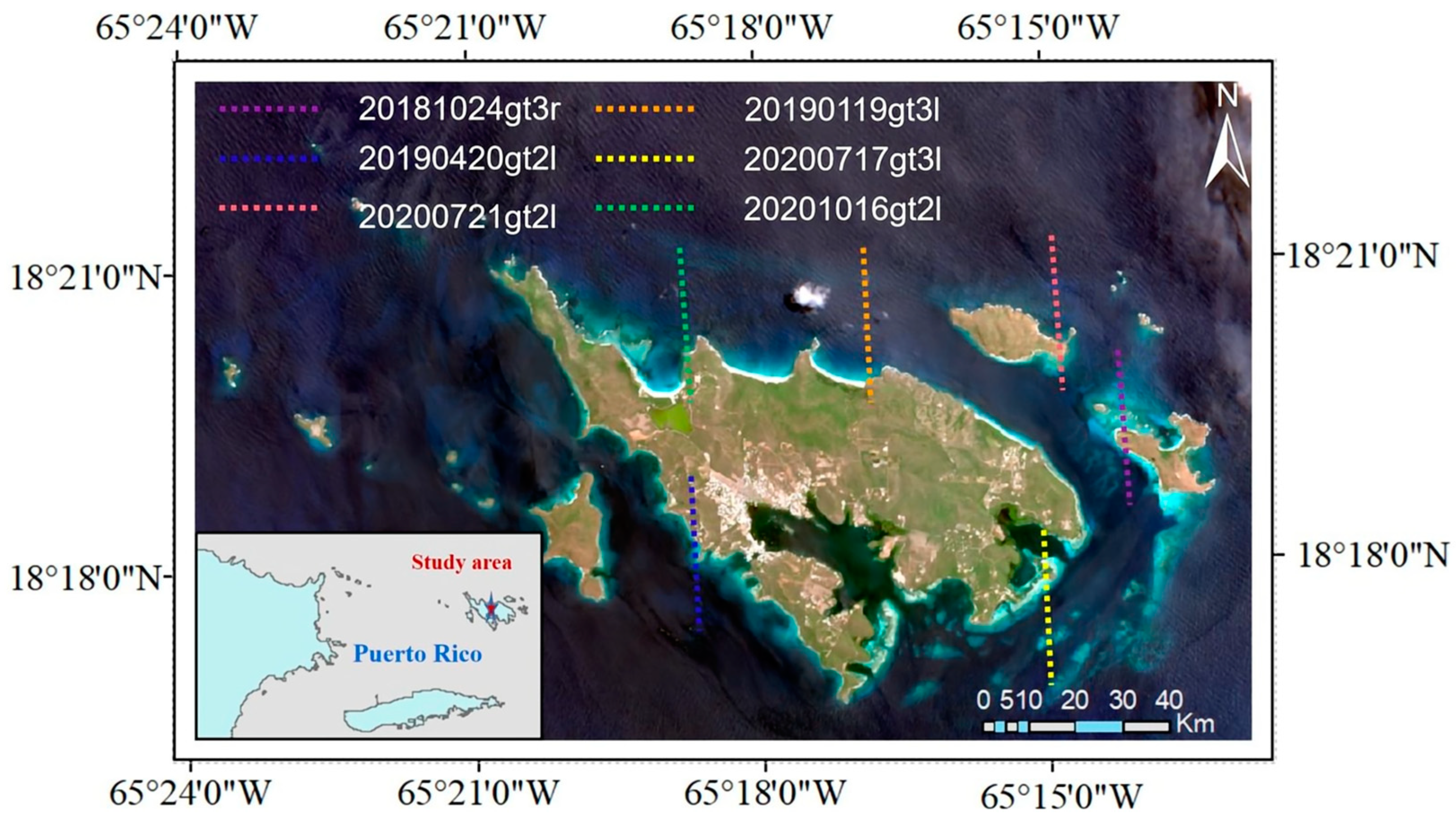
2.1. Study Area
2.2. ATL03 Dataset
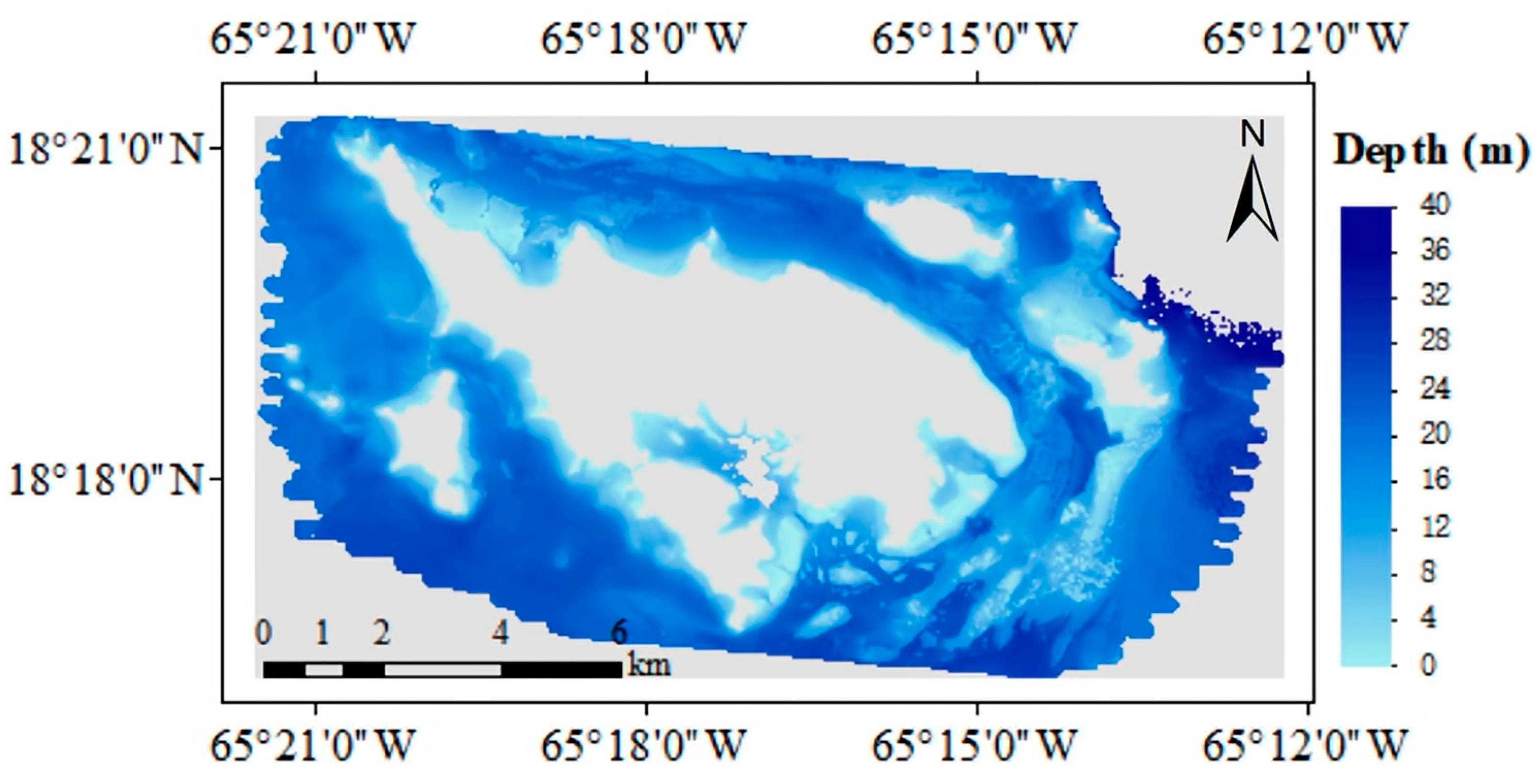
2.3. Reference ALB Data
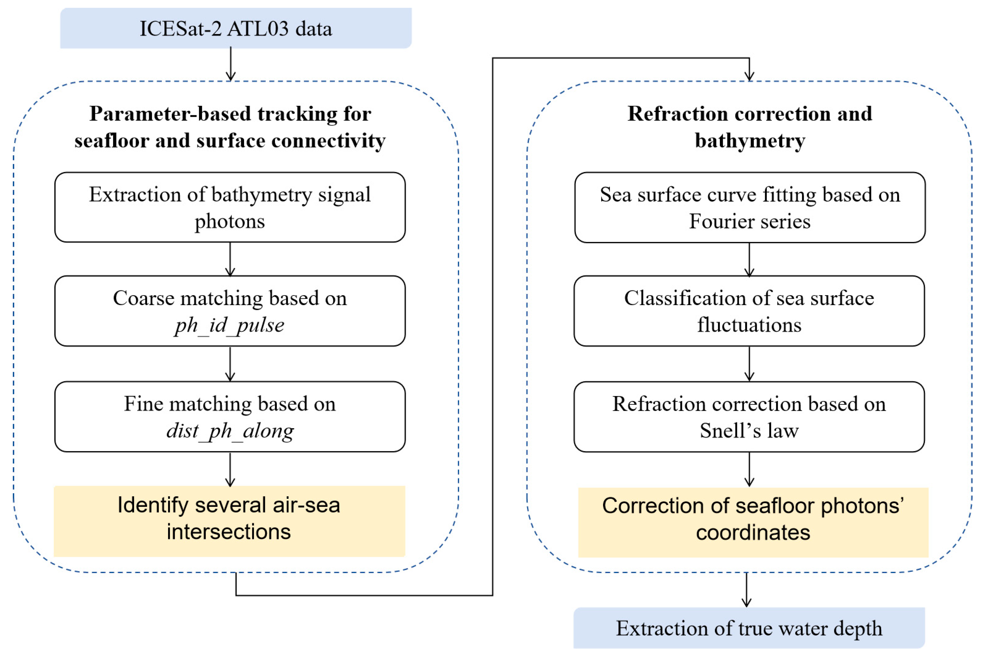
3. Methods
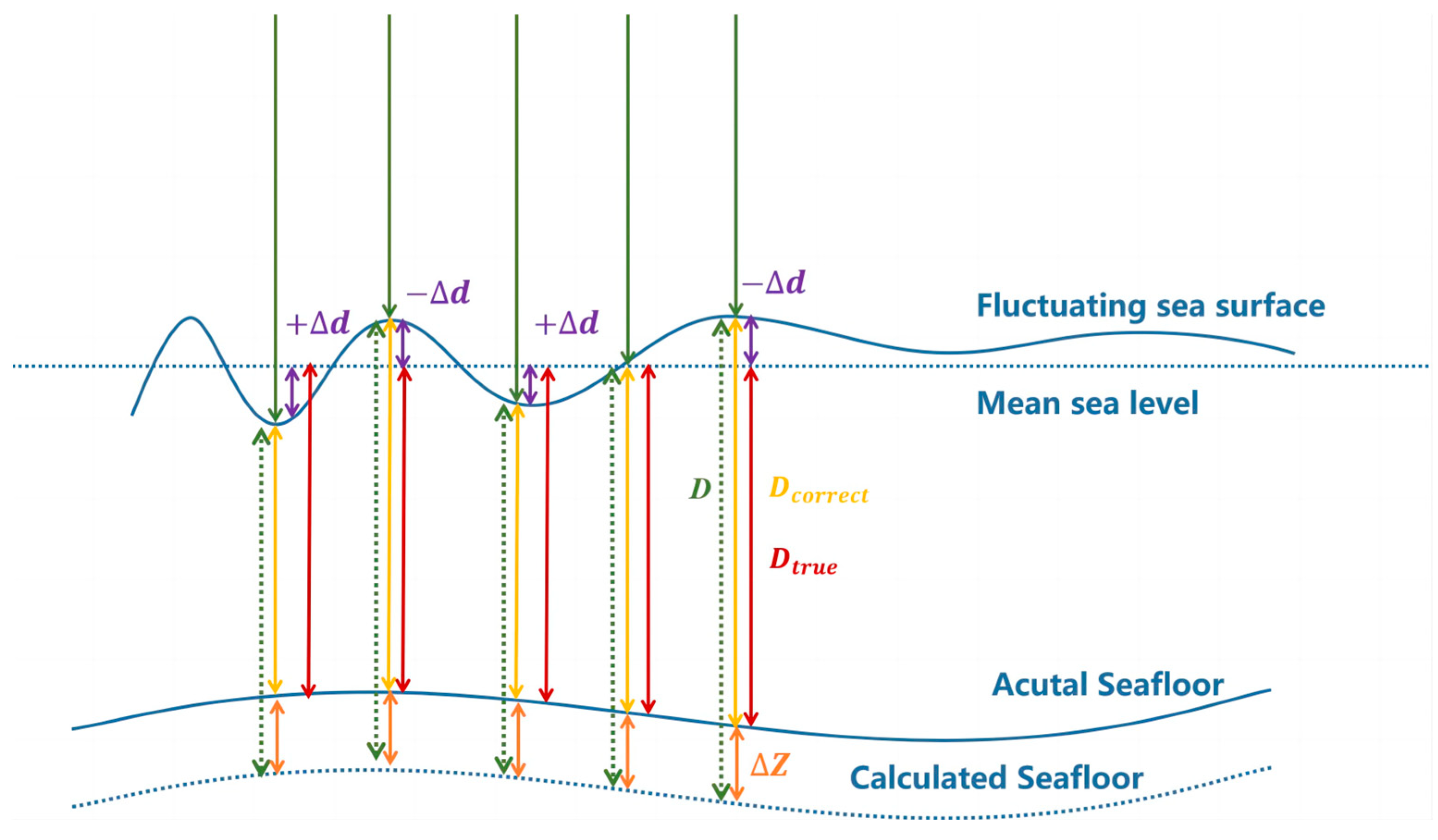
3.1. Refraction Correction and Bathymetry Model
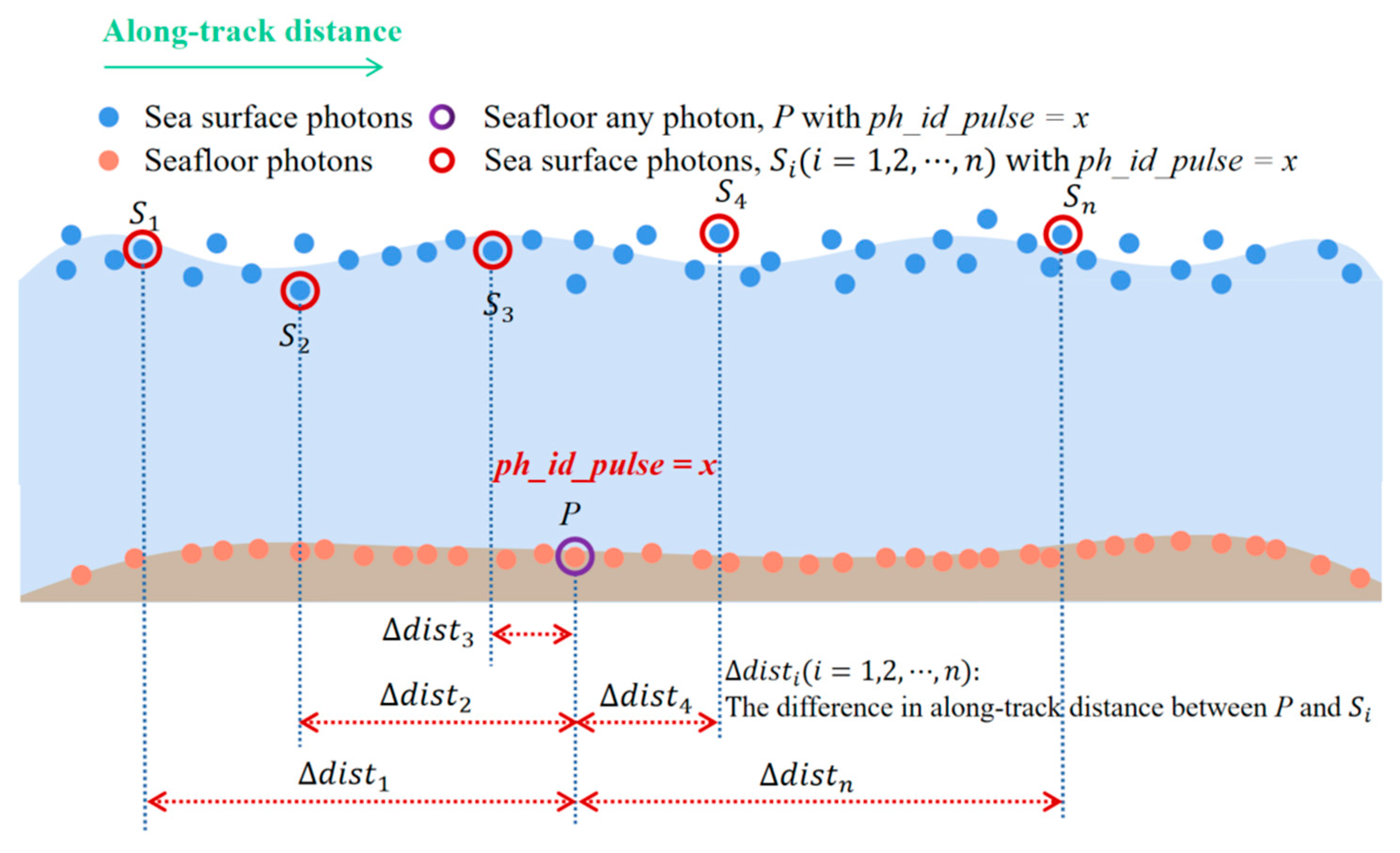
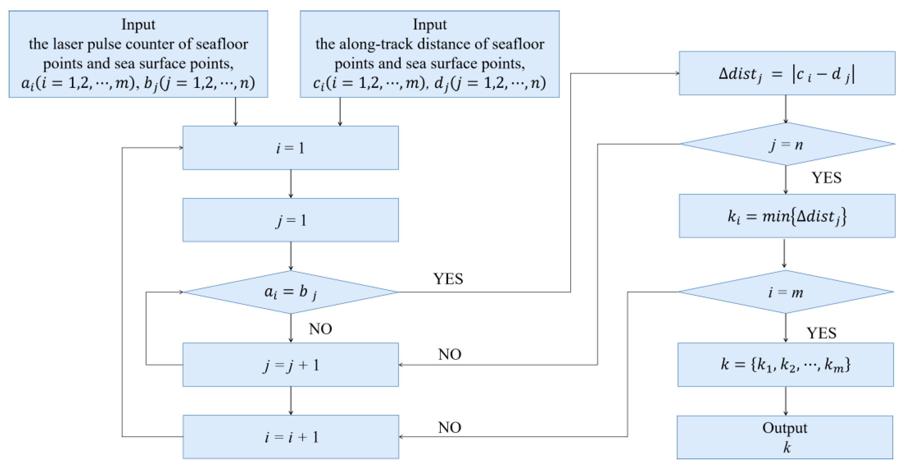
3.2. Parameter-Based Tracking for Seafloor and Surface Connectivity
4. Results
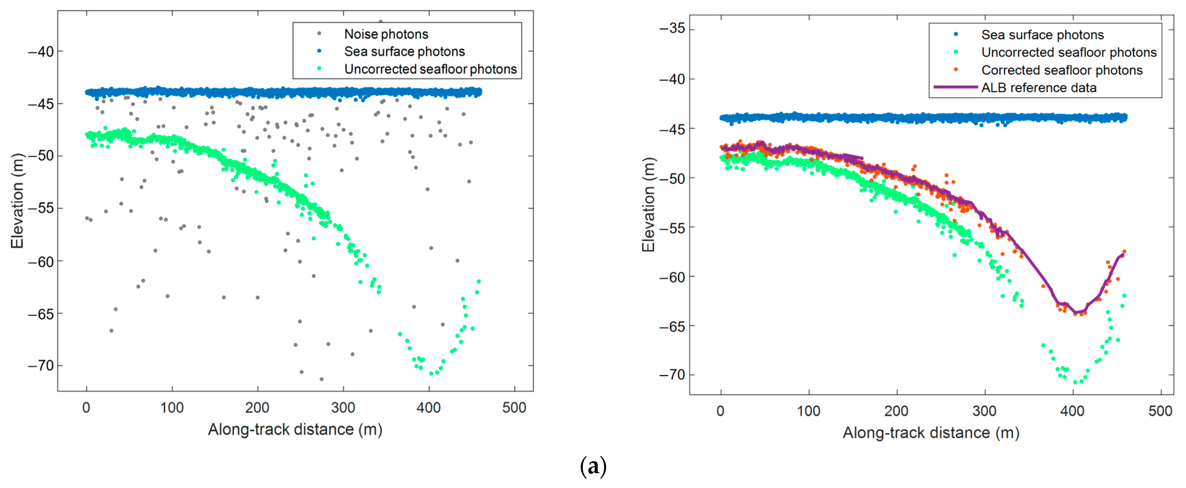
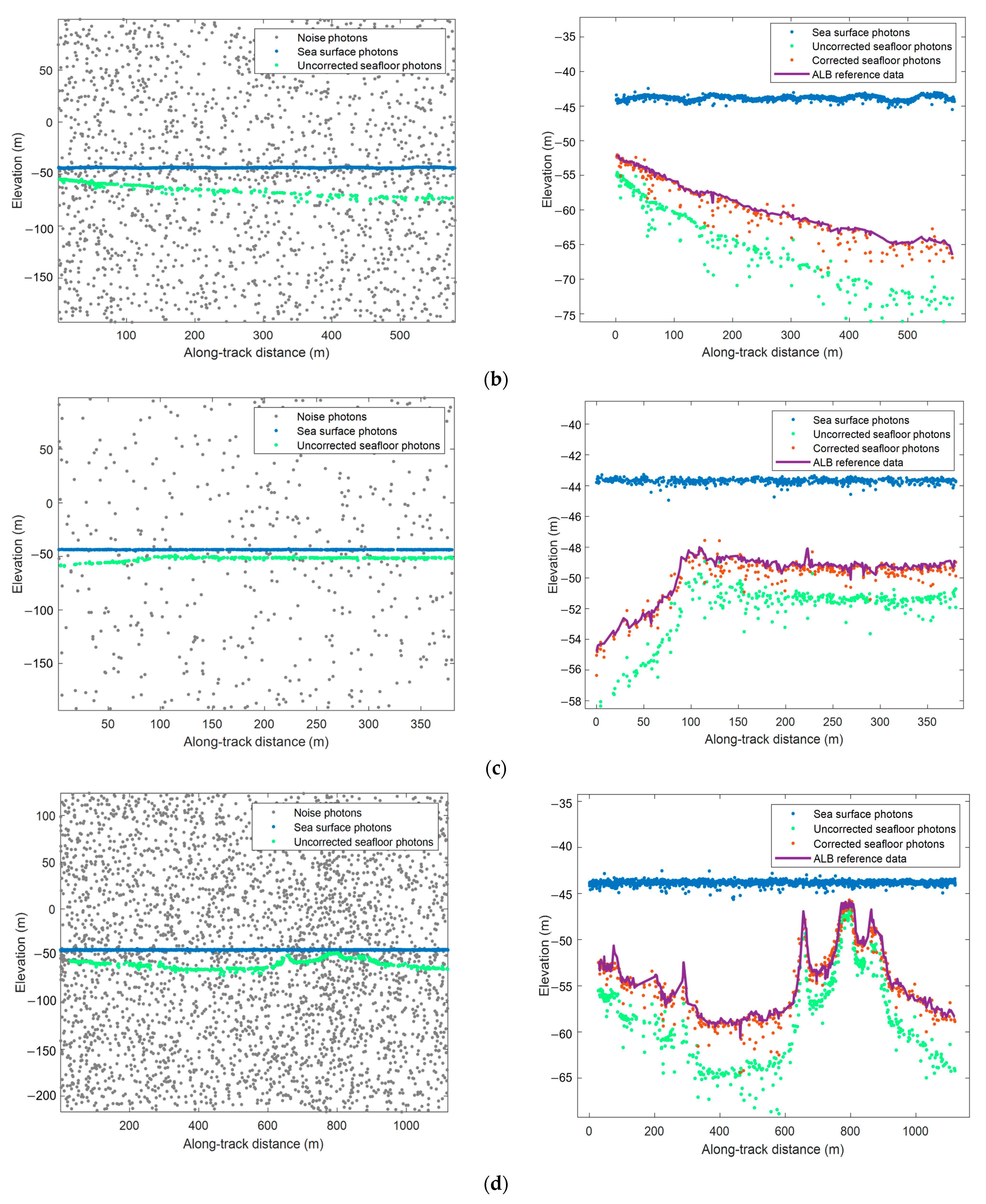
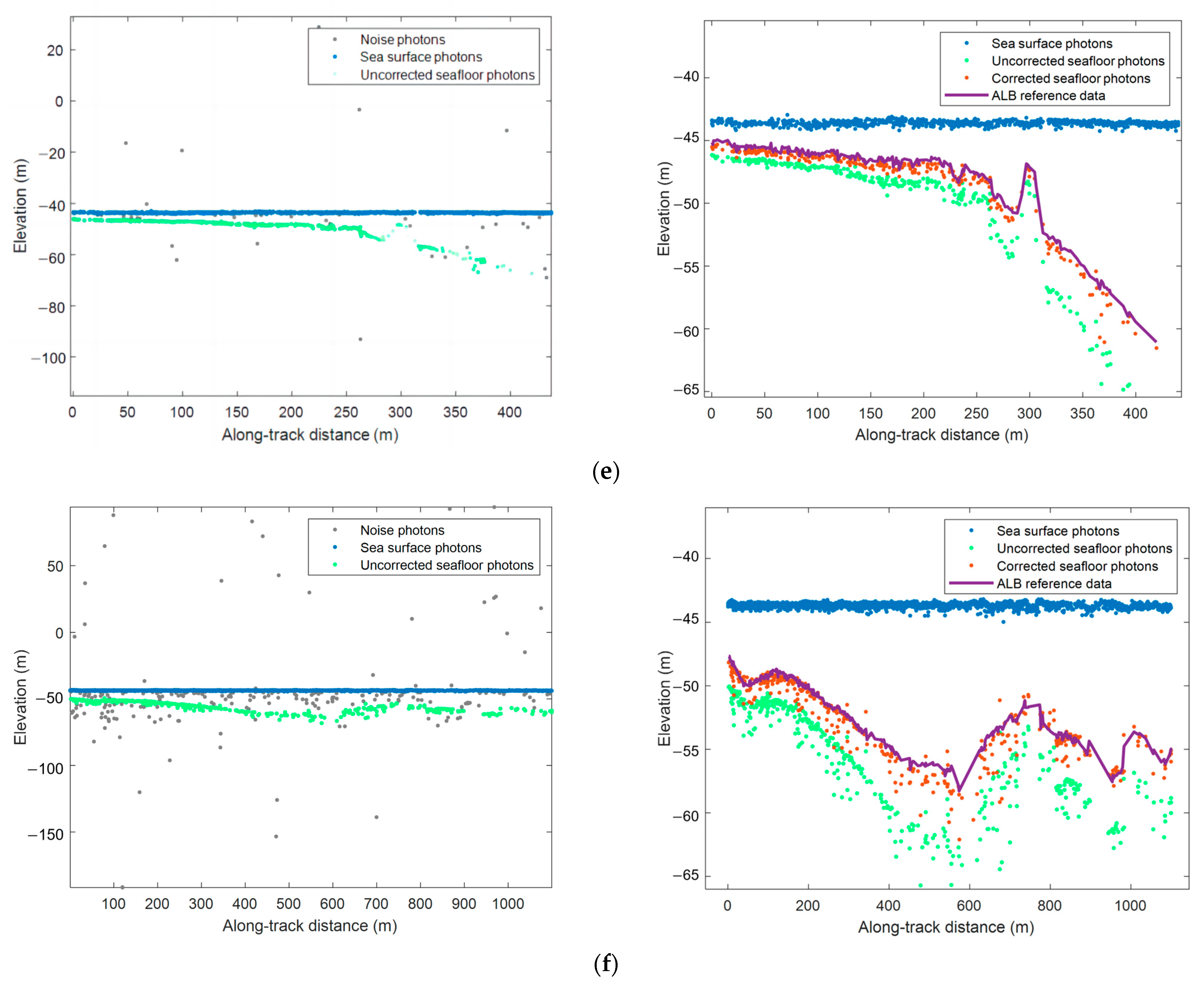
4.1. Refraction Correction and Bathymetry Results for Seafloor Signal Photons
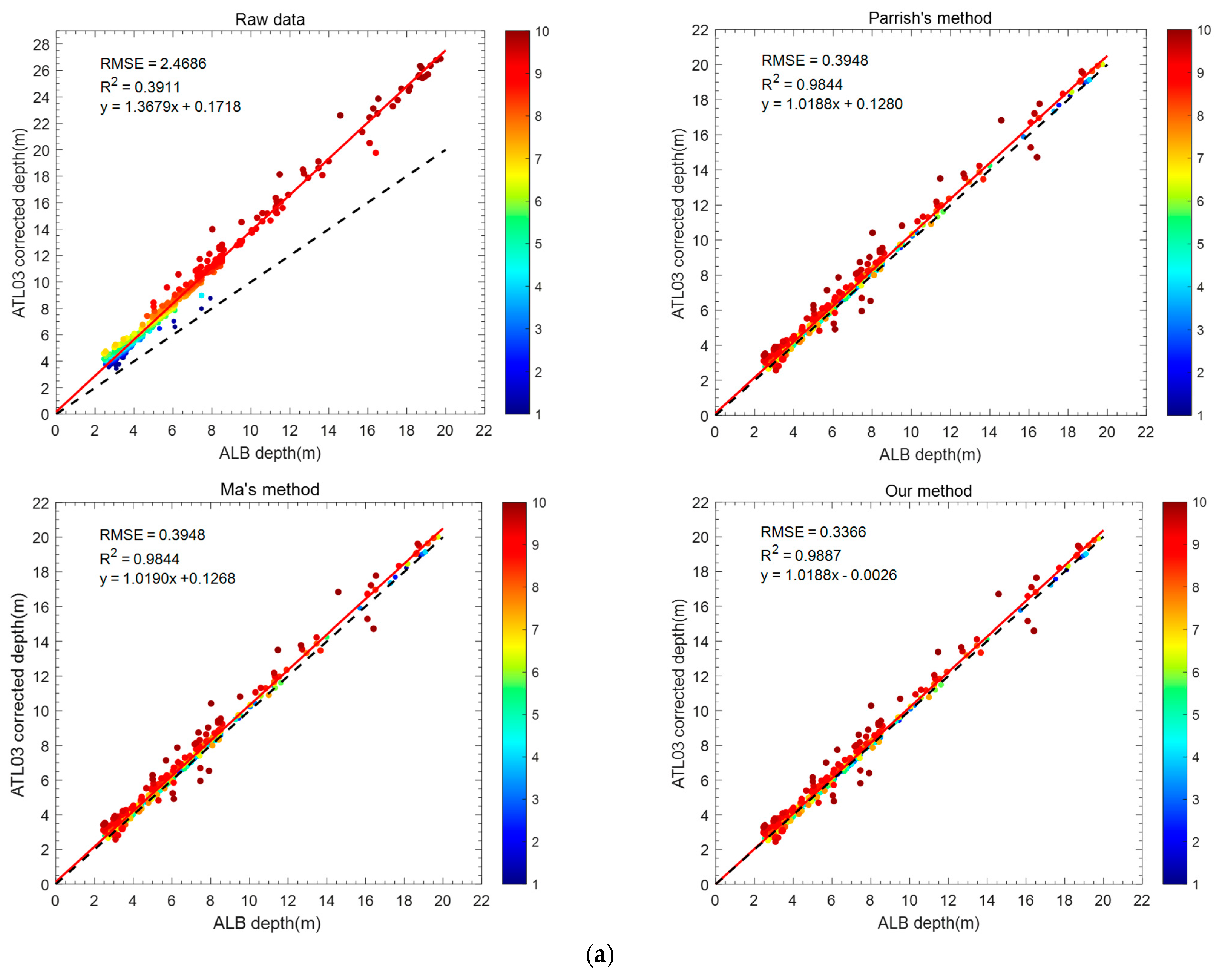
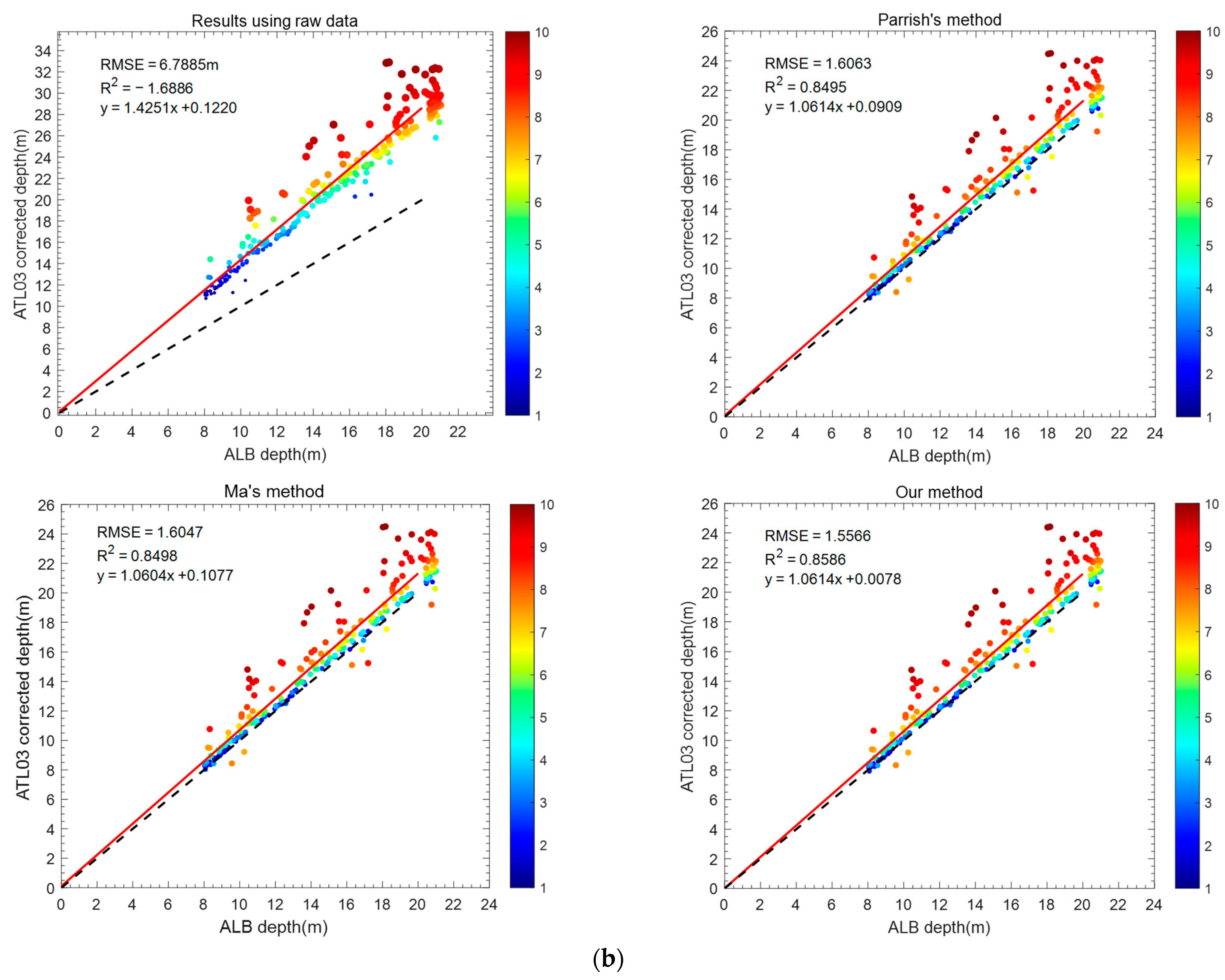
4.2. Validation of Refraction Correction and Bathymetry
5. Discussion
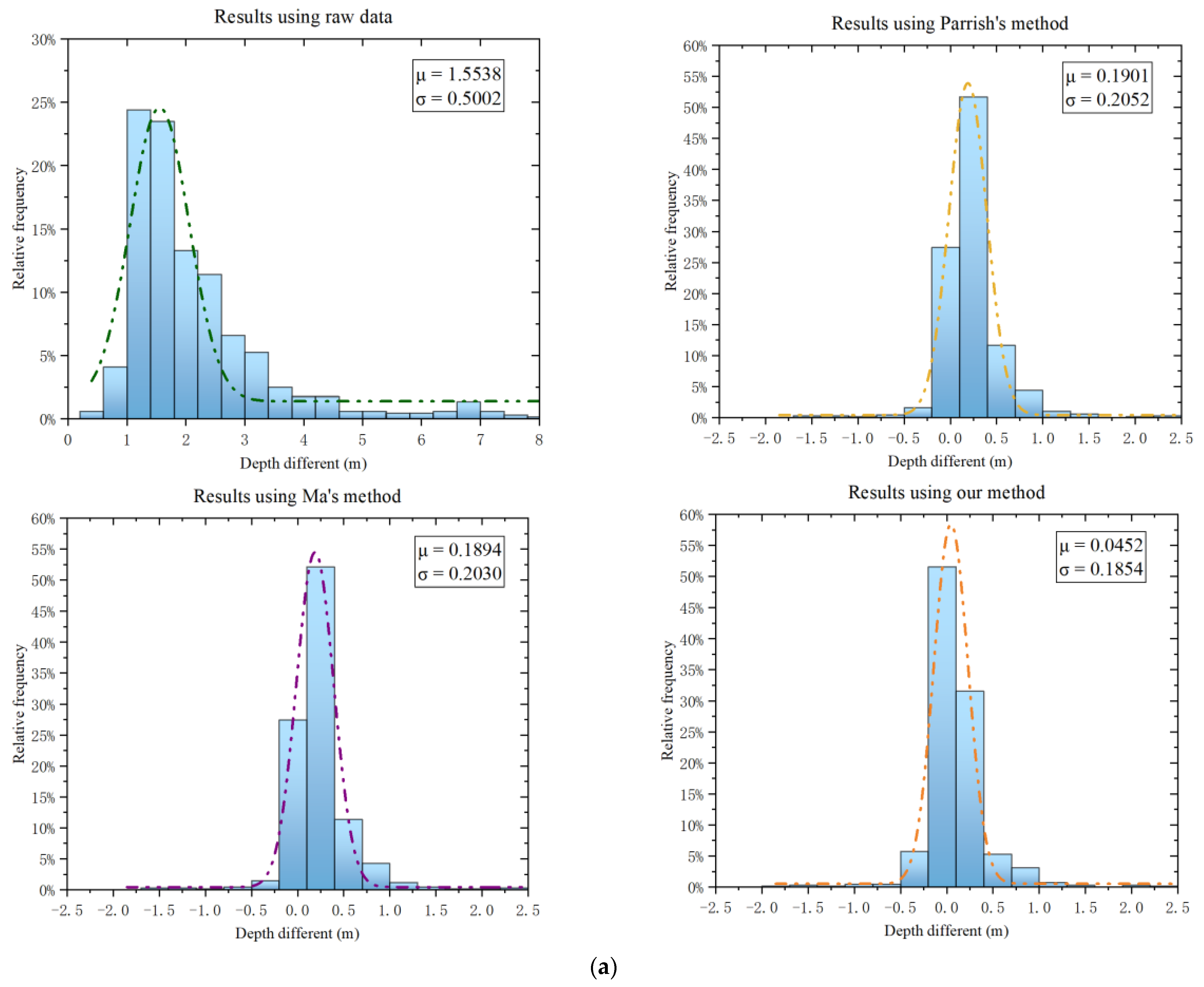
5.1. Error Analysis of Bathymetry
5.2. Analyzing the Accuracy of Refraction Correction Methods for Different Water Depth Intervals
6. Conclusions
Author Contributions
Funding
Data Availability Statement
Acknowledgments
Conflicts of Interest
References
- Dong, Y.; Liu, Y.; Hu, C.; Xu, B. Coral reef geomorphology of the Spratly Islands: A simple method based on time-series of Landsat-8 multi-band inundation maps. ISPRS J. Photogramm. Remote Sens. 2019, 157, 137–154. [Google Scholar] [CrossRef]
- Andersen, J.H.; Al-Hamdani, Z.; Harvey, E.T.; Kallenbach, E.; Murray, C.; Stock, A. Relative impacts of multiple human stressors in estuaries and coastal waters in the North Sea-Baltic Sea transition zone. Sci. Total Environ. 2020, 704, 135316. [Google Scholar] [CrossRef] [PubMed]
- Zhang, X.H.; Chen, Y.F.; Le, Y.; Zhang, D.F.; Yan, Q.; Dong, Y.S.; Han, W.; Wang, L.Z. Nearshore Bathymetry Based on ICESat-2 and Multispectral Images: Comparison Between Sentinel-2, Landsat-8, and Testing Gaofen-2. IEEE J. Sel. Top. Appl. Earth Obs. Remote Sens. 2022, 15, 2449–2462. [Google Scholar] [CrossRef]
- Wang, Z.; Yang, X.; Su, F.; Zhang, H.; Yan, F.; Zhang, J. Remote Sensing Application in China’s Coastal Zones and Islands: Recent Progress and Some Suggestions. Strateg. Study CAE 2019, 21, 59–63. [Google Scholar] [CrossRef]
- Saylam, K.; Brown, R.A.; Hupp, J.R. Assessment of depth and turbidity with airborne Lidar bathymetry and multiband satellite imagery in shallow water bodies of the Alaskan North Slope. Int. J. Appl. Earth Obs. Geoinf. 2017, 58, 191–200. [Google Scholar] [CrossRef]
- Li, Y.; Gao, H.; Jasinski, M.F.; Zhang, S.; Stoll, J.D. Deriving High-Resolution Reservoir Bathymetry from ICESat-2 Prototype Photon-Counting Lidar and Landsat Imagery. IEEE Trans. Geosci. Remote Sens. 2019, 57, 7883–7893. [Google Scholar] [CrossRef]
- Schwarz, R.; Mandlburger, G.; Pfennigbauer, M.; Pfeifer, N. Design and evaluation of a full-wave surface and bottom-detection algorithm for LiDAR bathymetry of very shallow waters. ISPRS J. Photogramm. Remote Sens. 2019, 150, 1–10. [Google Scholar] [CrossRef]
- Markus, T.; Neumann, T.; Martino, A.; Abdalati, W.; Brunt, K.; Csatho, B.; Farrell, S.; Fricker, H.; Gardner, A.; Harding, D.; et al. The Ice, Cloud, and land Elevation Satellite-2 (ICESat-2): Science requirements, concept, and implementation. Remote Sens. Environ. 2017, 190, 260–273. [Google Scholar] [CrossRef]
- Caballero, I.; Stumpf, R.P. On the use of Sentinel-2 satellites and lidar surveys for the change detection of shallow bathymetry: The case study of North Carolina inlets. Coast. Eng. 2021, 169, 103936. [Google Scholar] [CrossRef]
- Babbel, B.J.; Parrish, C.E.; Magruder, L.A. ICESat-2 Elevation Retrievals in Support of Satellite-Derived Bathymetry for Global Science Applications. Geophys. Res. Lett. 2021, 48, e2020GL090629. [Google Scholar] [CrossRef]
- Hsu, H.-J.; Huang, C.-Y.; Jasinski, M.; Li, Y.; Gao, H.; Yamanokuchi, T.; Wang, C.-G.; Chang, T.-M.; Ren, H.; Kuo, C.-Y.; et al. A semi-empirical scheme for bathymetric mapping in shallow water by ICESat-2 and Sentinel-2: A case study in the South China Sea. ISPRS J. Photogramm. Remote Sens. 2021, 178, 1–19. [Google Scholar] [CrossRef]
- Zhang, G.; Chen, W.; Xie, H. Tibetan Plateau’s lake level and volume changes from NASA’s ICESat/ICESat-2 and Landsat Missions. Geophys. Res. Lett. 2019, 46, 13107–13118. [Google Scholar] [CrossRef]
- Abdalati, W.; Zwally, H.J.; Bindschadler, R.; Csatho, B.; Farrell, S.L.; Fricker, H.A.; Harding, D.; Kwok, R.; Lefsky, M.; Markus, T.; et al. The ICESat-2 Laser Altimetry Mission. Proc. IEEE 2010, 98, 735–751. [Google Scholar] [CrossRef]
- Albright, A.; Glennie, C. Nearshore Bathymetry from Fusion of Sentinel-2 and ICESat-2 Observations. IEEE Geosci. Remote Sens. Lett. 2021, 18, 900–904. [Google Scholar] [CrossRef]
- Parrish, C.E.; Magruder, L.A.; Neuenschwander, A.L.; Forfinski-Sarkozi, N.; Alonzo, M.; Jasinski, M. Validation of ICESat-2 ATLAS Bathymetry and Analysis of ATLAS’s Bathymetric Mapping Performance. Remote Sens. 2019, 11, 1634. [Google Scholar] [CrossRef]
- Thomas, N.; Lee, B.; Coutts, O.; Bunting, P.; Lagomasino, D.; Fatoyinbo, L. A Purely Spaceborne Open Source Approach for Regional Bathymetry Mapping. IEEE Trans. Geosci. Remote Sens. 2022, 60, 4708109. [Google Scholar] [CrossRef]
- Wang, B.; Ma, Y.; Zhang, J.; Zhang, H.; Zhu, H.; Leng, Z.; Zhang, X.; Cui, A. A noise removal algorithm based on adaptive elevation difference thresholding for ICESat-2 photon-counting data. Int. J. Appl. Earth Obs. Geoinf. 2023, 117, 103207. [Google Scholar] [CrossRef]
- Yang, F.; Su, D.; Ma, Y.; Feng, C.; Yang, A.; Wang, M. Refraction Correction of Airborne LiDAR Bathymetry Based on Sea Surface Profile and Ray Tracing. IEEE Trans. Geosci. Remote Sens. 2017, 55, 6141–6149. [Google Scholar] [CrossRef]
- Xu, N.; Ma, Y.; Zhang, W.; Wang, X.H.; Yang, F.; Su, D. Monitoring Annual Changes of Lake Water Levels and Volumes over 1984-2018 Using Landsat Imagery and ICESat-2 Data. Remote Sens. 2020, 12, 4004. [Google Scholar] [CrossRef]
- Ma, Y.; Xu, N.; Liu, Z.; Yang, B.; Yang, F.; Wang, X.H.; Li, S. Satellite-derived bathymetry using the ICESat-2 lidar and Sentinel-2 imagery datasets. Remote Sens. Environ. 2020, 250, 112047. [Google Scholar] [CrossRef]
- Ma, Y.; Xu, N.; Sun, J.; Wang, X.H.; Yang, F.; Li, S. Estimating water levels and volumes of lakes dated back to the 1980s using Landsat imagery and photon-counting lidar datasets. Remote Sens. Environ. 2019, 232, 111287. [Google Scholar] [CrossRef]
- Liu, C.; Qi, J.; Li, J.; Tang, Q.; Xu, W.; Zhou, X.; Meng, W. Accurate Refraction Correction-Assisted Bathymetric Inversion Using ICESat-2 and Multispectral Data. Remote Sens. 2021, 13, 4355. [Google Scholar] [CrossRef]
- Zhang, D.; Chen, Y.; Le, Y.; Dong, Y.; Dai, G.; Wang, L. Refraction and coordinate correction with the JONSWAP model for ICESat-2 bathymetry. ISPRS J. Photogramm. Remote Sens. 2022, 186, 285–300. [Google Scholar] [CrossRef]
- Chen, Y.; Zhu, Z.; Le, Y.; Qiu, Z.; Chen, G.; Wang, L. Refraction correction and coordinate displacement compensation in nearshore bathymetry using ICESat-2 lidar data and remote-sensing images. Opt. Express 2021, 29, 2411–2430. [Google Scholar] [CrossRef] [PubMed]
- Cao, B.; Fang, Y.; Gao, L.; Hu, H.; Jiang, Z.; Sun, B.; Lou, L. An active-passive fusion strategy and accuracy evaluation for shallow water bathymetry based on ICESat-2 ATLAS laser point cloud and satellite remote sensing imagery. Int. J. Remote Sens. 2021, 42, 2783–2806. [Google Scholar] [CrossRef]
- Xu, N.; Ma, Y.; Zhou, H.; Zhang, W.; Zhang, Z.; Wang, X.H. A Method to Derive Bathymetry for Dynamic Water Bodies Using ICESat-2 and GSWD Data Sets. IEEE Geosci. Remote Sens. Lett. 2022, 19, 1500305. [Google Scholar] [CrossRef]
- Mattia Mazzaretto, O.; Menendez, M.; Lobeto, H. A global evaluation of the JONSWAP spectra suitability on coastal areas. Ocean. Eng. 2022, 266, 112756. [Google Scholar] [CrossRef]
- Zhang, G.; Xu, Q.; Xing, S.; Li, P.; Zhang, X.; Wang, D.; Dai, M. A Noise-Removal Algorithm Without Input Parameters Based on Quadtree Isolation for Photon-Counting LiDAR. IEEE Geosci. Remote Sens. Lett. 2022, 19, 6501905. [Google Scholar] [CrossRef]
- Zhu, X.; Nie, S.; Wang, C.; Xi, X.; Lao, J.; Li, D. Consistency analysis of forest height retrievals between GEDI and ICESat-2. Remote Sens. Environ. 2022, 281, 113244. [Google Scholar] [CrossRef]


| Date | Track | Time (UTC) | Latitude Range (°N) |
|---|---|---|---|
| 24 October 2018 | gt3r | 07:29 | 18.3180–18.3221 |
| 19 January 2019 | gt3l | 15:14 | 18.3324–18.3376 |
| 20 April 2019 | gt2l | 10:54 | 18.2996–18.3030 |
| 17 July 2020 | gt3l | 13:13 | 18.2810–18.2910 |
| 21 July 2020 | gt2l | 01:08 | 18.3301–18.3340 |
| 16 October 2020 | gt2l | 08:53 | 18.3299–18.3398 |
| Dataset | Raw Data | Parrish’s [15] | Ma’s [20] | Ours | ||||
|---|---|---|---|---|---|---|---|---|
| RMSE/m | RMSE/m | RMSE/m | RMSE/m | |||||
| 20181024gt3r | 0.3911 | 2.4686 | 0.9844 | 0.3948 | 0.9844 | 0.3948 | 0.9887 | 0.3366 |
| 20190119gt3l | −1.6886 | 6.7885 | 0.8495 | 1.6063 | 0.8498 | 1.6047 | 0.8586 | 1.5566 |
| 20190420gt2l | −2.1283 | 2.5723 | 0.8706 | 0.5232 | 0.8705 | 0.5233 | 0.8727 | 0.5189 |
| 20200717gt3l | −0.3472 | 4.5165 | 0.8958 | 1.2561 | 0.8959 | 1.2552 | 0.8988 | 1.2379 |
| 20200721gt2l | 0.3632 | 2.5045 | 0.9516 | 0.6905 | 0.9518 | 0.6888 | 0.9557 | 0.6603 |
| 20201016gt2l | −1.5829 | 4.2464 | 0.7229 | 1.3908 | 0.7229 | 1.3909 | 0.7359 | 1.3579 |
| Dateset | Error Correction Method of Bathymetry | Error | ||
|---|---|---|---|---|
| Range | Mean | Standard Deviation | ||
| 20181024gt3r | raw data | [0.3721, 8.0055] | 1.5538 | 0.5002 |
| Parrish’s [15] | [−1.6918, 2.4010] | 0.1901 | 0.2052 | |
| Ma’s [20] | [−1.6862, 2.4037] | 0.1894 | 0.2030 | |
| ours | [−1.8224, 2.2705] | 0.0452 | 0.1854 | |
| 20190119gt3l | raw data | [1.7275, 14.8129] | 5.7841 | 2.1795 |
| Parrish’s [15] | [−1.9490, 6.4320] | 0.4157 | 0.2539 | |
| Ma’s [20] | [−1.9479, 6.4314] | 0.4089 | 0.2395 | |
| ours | [−2.0320, 6.3493] | 0.3371 | 0.2707 | |
| 20190420gt2l | raw data | [0.2895, 5.8635] | 2.1924 | 0.2853 |
| Parrish’s [15] | [−1.2883, 2.2441] | 0.2233 | 0.1995 | |
| Ma’s [20] | [−1.2846, 2.2431] | 0.2229 | 0.1974 | |
| ours | [−1.2951, 2.2375] | 0.2184 | 0.1994 | |
| 20200717gt3l | raw data | [−0.8652, 12.5306] | 4.0070 | 1.7007 |
| Parrish’s [15] | [−3.0447, 7.2198] | 0.2904 | 0.5356 | |
| Ma’s [20] | [−3.0515, 7.2107] | 0.2946 | 0.5388 | |
| ours | [−3.0851, 7.1794] | 0.2686 | 0.5507 | |
| 20200721gt2l | raw data | [0.8338, 10.3489] | 1.3500 | 0.0750 |
| Parrish’s [15] | [−0.6951, 4.4112] | 0.4371 | 0.1774 | |
| Ma’s [20] | [−0.6881, 4.4181] | 0.4368 | 0.1737 | |
| ours | [−0.7366, 4.3697] | 0.4053 | 0.1729 | |
| 20201016gt2l | raw data | [0.5431, 17.6839] | 3.8980 | 0.6138 |
| Parrish’s [15] | [−2.0084, 11.8424] | 0.3261 | 0.2075 | |
| Ma’s [20] | [−1.9900, 11.8291] | 0.3839 | 0.2404 | |
| ours | [−2.0772, 11.7736] | 0.2985 | 0.0923 | |
| Dateset | Error Correction Method of Bathymetry | Division of Depth, RMSE of Each Segmentation (m) | ||||
|---|---|---|---|---|---|---|
| 20181024gt3r | [2, 4] | [4, 6] | [6, 8] | [8, 10] | >10 | |
| raw data | 0.9709 | 1.4238 | 2.0015 | 2.5165 | 4.4315 | |
| Parrish’s [15] | 0.4663 | 0.7341 | 0.8357 | 1.3083 | 2.0290 | |
| Ma’s [20] | 0.2812 | 0.3061 | 0.4214 | 0.5354 | 0.8042 | |
| ours | 0.2202 | 0.2784 | 0.3489 | 0.4537 | 0.6898 | |
| 20190119gt3l | [8, 10] | [10, 12] | [12, 14] | [14, 16] | >16 | |
| raw data | 3.0396 | 3.6663 | 4.6573 | 7.5903 | ||
| Parrish’s [15] | 0.4746 | 0.8646 | 1.0909 | 1.7246 | 1.9882 | |
| Ma’s [20] | 0.4976 | 0.8577 | 1.0681 | 1.7197 | 2.0265 | |
| ours | 0.4445 | 0.8099 | 1.0366 | 1.6992 | 1.9704 | |
| 20190420gt2l | [4, 6] | [6, 8] | [8, 10] | >10 | ||
| raw data | 0.3771 | 2.1623 | 3.1743 | 3.5238 | ||
| Parrish’s [15] | 0.3532 | 0.9886 | 0.4299 | 0.5578 | ||
| Ma’s [20] | 0.3536 | 1.0055 | 0.4319 | 0.5470 | ||
| ours | 0.3490 | 0.9828 | 0.4262 | 0.5328 | ||
| 20200717gt3l | [2, 4] | [4, 6] | [6, 8] | [8, 10] | >10 | |
| raw data | 1.0454 | 1.9483 | 2.9535 | 2.7689 | 5.0541 | |
| Parrish’s [15] | 0.5256 | 1.4353 | 1.2397 | 0.7974 | 1.4582 | |
| Ma’s [20] | 0.5264 | 1.4348 | 1.2393 | 0.7970 | 1.4569 | |
| ours | 0.5051 | 1.4119 | 1.2151 | 0.7917 | 1.4361 | |
| 20200721gt2l | [2, 4] | [4, 6] | [6, 8] | [8, 10] | >10 | |
| raw data | 1.2173 | 1.7142 | 2.2029 | 3.3939 | 5.3464 | |
| Parrish’s [15] | 0.4538 | 0.5732 | 1.1429 | 0.6255 | 1.4349 | |
| Ma’s [20] | 0.4502 | 0.5725 | 1.1396 | 0.6198 | 1.4367 | |
| ours | 0.4153 | 0.5430 | 1.1099 | 0.6493 | 1.4401 | |
| 20201016gt2l | [4, 6] | [6, 8] | [8, 10] | [10, 12] | >12 | |
| raw data | 2.2079 | 2.8147 | 3.2903 | 5.4403 | ||
| Parrish’s [15] | 0.4234 | 0.8270 | 0.8701 | 1.0594 | 2.7469 | |
| Ma’s [20] | 0.4184 | 0.8301 | 0.8675 | 1.0641 | 2.7481 | |
| ours | 0.3871 | 0.8194 | 0.8162 | 1.0280 | 2.3496 | |
Disclaimer/Publisher’s Note: The statements, opinions and data contained in all publications are solely those of the individual author(s) and contributor(s) and not of MDPI and/or the editor(s). MDPI and/or the editor(s) disclaim responsibility for any injury to people or property resulting from any ideas, methods, instructions or products referred to in the content. |
© 2023 by the authors. Licensee MDPI, Basel, Switzerland. This article is an open access article distributed under the terms and conditions of the Creative Commons Attribution (CC BY) license (https://creativecommons.org/licenses/by/4.0/).
Share and Cite
Chen, L.; Xing, S.; Zhang, G.; Guo, S.; Gao, M. Refraction Correction Based on ATL03 Photon Parameter Tracking for Improving ICESat-2 Bathymetry Accuracy. Remote Sens. 2024, 16, 84. https://doi.org/10.3390/rs16010084
Chen L, Xing S, Zhang G, Guo S, Gao M. Refraction Correction Based on ATL03 Photon Parameter Tracking for Improving ICESat-2 Bathymetry Accuracy. Remote Sensing. 2024; 16(1):84. https://doi.org/10.3390/rs16010084
Chicago/Turabian StyleChen, Li, Shuai Xing, Guoping Zhang, Songtao Guo, and Ming Gao. 2024. "Refraction Correction Based on ATL03 Photon Parameter Tracking for Improving ICESat-2 Bathymetry Accuracy" Remote Sensing 16, no. 1: 84. https://doi.org/10.3390/rs16010084