Technical Note

Hyperspectral Imaging Spectroscopy for Non-Destructive Determination of Grape Berry Total Soluble Solids and Titratable Acidity

1
School of Agriculture and Environment, Massey University, Palmerston North 4410, New Zealand
2
Massey Agri-Food (MAF) Digital Lab., Massey University, Palmerston North 4410, New Zealand
*
Author to whom correspondence should be addressed.
Remote Sens. 2024, 16(10), 1655; https://doi.org/10.3390/rs16101655
Submission received: 22 March 2024 / Revised: 26 April 2024 / Accepted: 4 May 2024 / Published: 7 May 2024
(This article belongs to the Special Issue Image Change Detection Research in Remote Sensing II)

Abstract

:
Wine grape quality heavily influences the price received for a product. Hyperspectral imaging has the potential to provide a non-destructive technique for predicting various enological parameters. This study aims to explore the feasibility of applying hyperspectral imaging to measure the total soluble solids (TSS) and titratable acidity (TA) in wine grape berries. A normalized difference spectral index (NDSI) spectral preprocessing method was built and compared with the conventional preprocessing method: multiplicative scatter correction and Savitzky–Golay smoothing (MSC+SG). Different machine learning models were built to examine the performance of the preprocessing methods. The results show that the NDSI preprocessing method demonstrated better performance than the MSC+SG preprocessing method in different classification models, with the best model correctly classifying 93.8% of the TSS and 84.4% of the TA. In addition, the TSS can be predicted with moderate performance using support vector regression (SVR) and MSC+SG preprocessing with a root mean squared error (RMSE) of 0.523 °Brix and a coefficient of determination (R2) of 0.622, and the TA can be predicted with moderate performance using SVR and NDSI preprocessing (RMSE = 0.19%, R2 = 0.525). This study demonstrates that hyperspectral imaging data and NDSI preprocessing have the potential to be a method for grading wine grapes for producing quality wines.

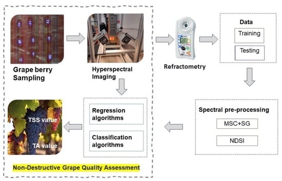
Graphical Abstract

1. Introduction

The quality of wine is strongly related to the compounds of the grape during harvesting. Traditionally, grape maturity is monitored by measuring grapes’ TSS and TA values. The TSS of grape berries directly affects the potential alcohol concentration, fermentable sugar concentration and flavor profile of the subsequent wine [1]. The TA is the concentration of organic acids present in the berries, such as tartaric acid, malic acid and citric acid, which are responsible for the overall sour taste of the subsequent wine [2]. These two enological parameters determine the optimal timing for grape harvesting and, consequently, the quality of the resulting wine. Currently, the measurement of a grape’s TSS and TA is destructive, involving handheld refractometers or traditional chemical analysis in laboratory settings. Due to differences in the position and orientation of the berries within each berry cluster, the quality of the berries varies spatially at the cluster level [3]. Most growers adopt a uniform harvesting approach, collecting grapes of varying quality together and processing them into wine. However, this production method may diminish winery profitability, as the inclusion of lower-quality berries during the production process can diminish the overall wine quality and subsequently lower its market value [4]. Obtaining the spatial variation in grape quality would require a large number of destructive measurements using the traditional method. The use of destructive measurement methods for the TSS and TA in a large number of grapes is not feasible for wine industry production as normally, viticulturists sample 200 berries per block to represent the whole block’s grape quality. Consequently, using a noninvasive and rapid method such as hyperspectral imaging (HSI) could provide a method to measure the TSS and TA in large numbers of grapes.
HSI is a non-destructive technique that combines conventional imaging with spectroscopy to capture and analyze the spatial and spectral information of objects [5]. HSI is commonly used in reflectance, transmittance and interactance modes. Among these modes, the reflectance mode is the most frequently used one for analyzing grape berries [6]. In reflectance mode, the light source directly illuminates the object’s surface, and the detector records information regarding the intensity of the light reflected by the objects, which varies according to the wavelength. Several studies have investigated using laboratory-based HSI technology to determine the following enological parameters: the TSS, TA, pH and anthocyanins [1,7,8]. One study used a laboratory-based HSI system in reflectance mode to predict grapes’ TSS values in Portugal [1]. Through the development of prediction models based on PLSR and neural networks, a prediction performance (R2) of up to 0.95 was achieved. The laboratory-based HSI system, combined with an SVR model, was employed to predict the anthocyanin concentration, pH index and TSS in whole grape berries. Determination coefficients (R2) of 0.89 (RMSE = 35.6 mg·L−1), 0.81 (RMSE = 0.25) and 0.90 (RMSE = 3.19 °Brix) were obtained for estimation of the anthocyanin concentration, pH index and TSS, respectively. These two studies highlight the potential of using HSI to predict the enological parameters in a rapid and noninvasive way. However, it is worth noting that the HSI systems commonly used in existing research primarily operate within the visible (VIS) and near-infrared (NIR) region (400–1000 nm) [1,8] (Gomes et al., 2017; Silva et al., 2018). Several studies explored the reflectance responses of grape berries in the short-wave infrared region (SWIR, 1400–3000 nm) and indicated the potential for predicting the enological parameters in the NIR and SWIR regions [7,9,10,11]. One study used a handheld spectroradiometer with a spectral range from 1600 to 2400 nm to predict a grape’s TSS within a lab setting [11]. The resultant prediction performance yielded an R2 value of 0.91 and an RMSE value of 1.42 °Brix.
Most previous studies used regression models to predict the grape TSS or TA, while the main objective of determining grape quality is classifying berries into two groups (ripe and unripe berries). The classification algorithms are important for distinguishing the quality of grapes. For example, one study explored a spectroradiometer (350–2500 nm) combined with various supervised classification methods to distinguish the maturation stages of wine grapes and obtained 93.15% accuracy [12]. In addition, several studies have reported using a spectroradiometer to classify grape quality based on the TSS or TA [13,14]. Compared with a spectroradiometer, the HSI system can provide more spatial information and is also easy to install on a berry sorting system for industrial application. Therefore, it is important to explore the potential of using the combination of HSI and classification algorithms to distinguish grape quality.
Machine learning has been widely applied in analyzing hyperspectral data, as hyperspectral imaging can provide a large amount of information with high complexity. However, many machine learning models are called “black boxes”, as the decision-making process of these models is often deemed uninterpretable [15,16]. Many interpretation methods have been developed with the aim to identify the features that contribute most to the model’s predictive performance. In grape studies, this can be useful to better understand the relevance of the specific wavelength for predicting different enological parameters [16].
This study aims to develop and evaluate the non-destructive and rapid prediction of two important compositional parameters, namely the TSS and TA, using NIR-SWIR hyperspectral imaging. The specific objectives were (1) to develop regression models to predict a grape’s TSS and TA using the combination of HSI and machine learning algorithms; (2) to develop classification models to distinguish grape quality and (3) to identify the spectral signatures which contribute most to the model’s performance.

2. Materials and Methods

2.1. Sample Acquisition

Samples of pinot noir grapes were collected three times during the pre-harvest stages in 2022 at a vineyard in Martinborough (41°13′8.73″S, 175°27′36.23″E), New Zealand. The vineyard features a cool, moist and temperate climate [17]. Random selection was employed to choose a total of 112 grapevines during the study period (Table 1). From each grapevine, three grape bunches were randomly selected (Figure 1). Subsequently, three berries were obtained from the top, middle and bottom within each bunch cluster and placed in labeled plastic bags immediately. Each sampled grapevine provided 9 berries to meet the minimum standards for subsequent TA and TSS measurements. The collected samples were immediately sent to a laboratory for hyperspectral spectrum analysis and chemical determination of the TSS and TA values. All samples were stored at 4 °C until beginning the hyperspectral imaging analysis.

2.2. Hyperspectral Image Acquisition and Analysis

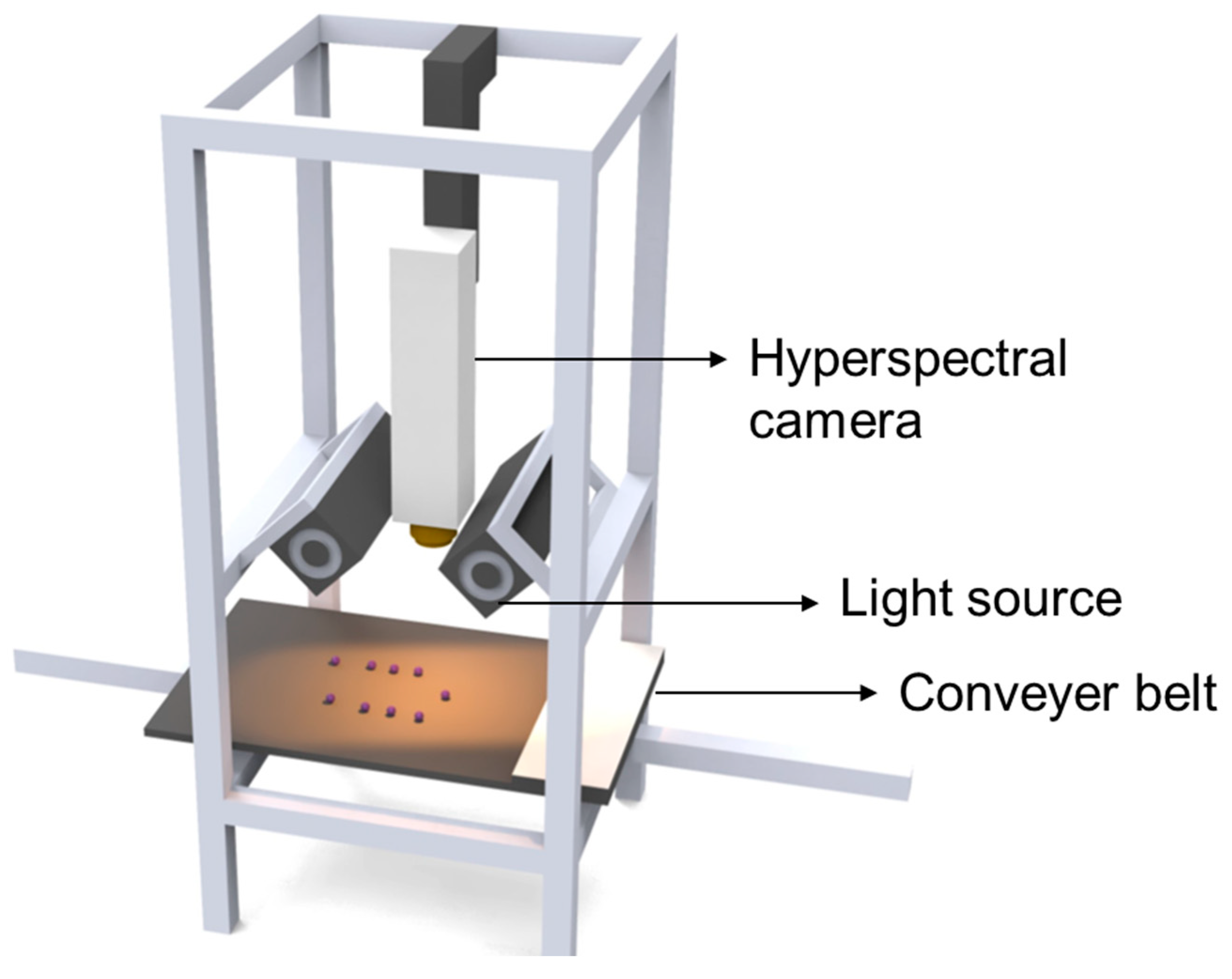
A Specim SWIR HSI system (Specim, Oulu, Finland) operating in reflectance mode was used to acquire images containing the NIR to SWIR spectra, ranging from 1000 to 2500 nm and comprising 288 spectral bands (Figure 2). The Specim SWIR is a pushbroom instrument which can capture images consisting of 384 spatial pixels. Two 50 watt tungsten halogen lamps were positioned at a 45 degree angle on both sides of the camera to provide illumination primarily focused on the grape samples for spatial information acquisition during scanning (Figure 2). The camera was situated 300 mm away from the objective base, and the imaging process was conducted using Specim Lumo software (5.6.0) within a dark room at room temperature. Each image was acquired at a rapid rate of 29 frames per second, with an exposure time of 2 ms. The grape berries were placed on a computer-controlled conveyor belt (with black light-absorbing material), which ensured consistent movement at a constant speed of 15 mm/s during the measurement process. A total of 112 images, each containing 9 fresh berries, were obtained using this HSI system (resulting in 112 samples).
To obtain surface reflectance from the raw hyperspectral images, two calibration steps were carried out using dark current and white reflectance. The dark current calibration involved closing the camera lens with a non-reflective, opaque black cap to capture the dark current values. For the white reference calibration, a white panel coated with barium sulfate, known for its near-perfect surface reflectance, was used. The reflectance value is computed as follows:
R λ = R r a w   λ R d a r k   ( λ ) R w h i t e   λ R d a r k   ( λ )
where R r a w   ( λ ) represents the intensity of the light reflected from the objective at a wavelength λ and R d a r k   ( λ ) and R w h i t e   ( λ ) represent the dark current and white reflectance at a wavelength λ, respectively.
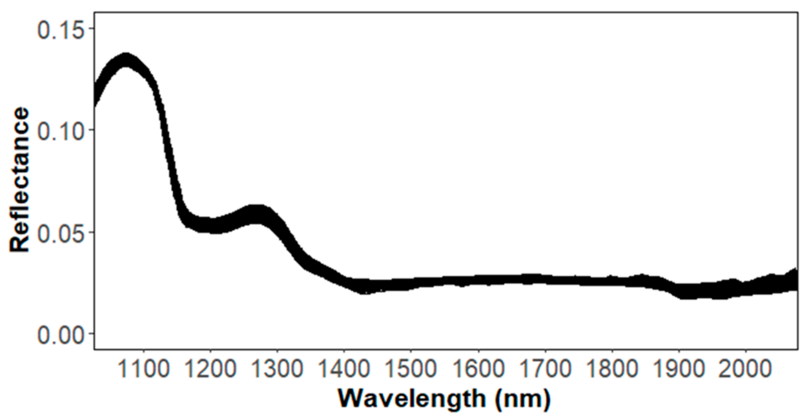
The hyperspectral images were processed by Environment for Visualizing Images (ENVI) V 5.6 software (Research Systems Inc., Boulder, CO, USA). A region of interest (ROI) was defined in the middle portion of each berry, and subsequently, the average spectrum of these ROIs was calculated to be used as the predictor variable for the prediction model (Figure 3). The average value of the nine grapes in each image was calculated to represent one sample. The ellipsoidal shape of the fruit resulted in the presence of shadows around the edges of each fruit, where the lighting was insufficient to fully illuminate the area. As a result, these shadowed regions were excluded from the selection of ROIs.
The resulting hyperspectral images exhibited various random noise, which was generate from the sensor or quantization process. The noise significantly degraded the quality of the spectral data and the overall prediction performance [18]. Before building the estimation model, multiplicative scatter correction and the Savitzky–Golay smoothing (MSC+SG) spectral preprocessing method were applied to the raw reflectance data to decrease the influence of the random noise and surface scattering. The mean of the data set was selected as the reference spectrum. Additionally, the normalized difference spectral index (NDSI) was also used to process raw reflectance data. The NDSI was calculated as follows:
N D S I = R x R y R x + R y
where R x and R y represent the reflectance at wavelengths x and y , respectively.
The Pearson’s coefficient correlation between the NDSI and TSS as well as the TA was calculated. The Pearson’s coefficient correlation ranges from +1 to −1. The closer it is to ±1, the stronger the correlation between the NDSI, TSS and TA. An NDSI with coefficients higher than 0.5 was selected for building the further regression and classification model.

2.3. Enological Parameter Measurements

After acquiring each hyperspectral image, the enological parameters of the grape berries were measured in the Massey AgriFood Digital Lab at Massey University in Palmerston North. Firstly, nine grape berries were squeezed together into juice. Then, we applied 0.2 mL of the collected juice onto a portable digital refractometer (PAL-BX/ACID F5 Digital Refractometer, ATAGO Co., Ltd., Tokyo, Japan) to measure the TSS value (°Brix). The refractometer is capable of measuring 0–60% °Brix (0.1% resolution) and 0.1–8.8% (0.01% resolution) acid. After measuring the TSS, we used reverse osmosis (RO) water to rinse the refractometer prism and then dried it with absorbent cleaning paper. The TA value was measured by a digital refractometer. We poured 1.00 g of grape juice into a beaker and diluted it with RO water at a ratio of 1:50. Then, we placed the 0.3 mL diluted sample onto the transparent prism surface of the refractometer and recorded the acidity (%) value.

2.4. Data Analysis

Before application of the prediction model, anomalous sample and spectral outlier detection was performed based on the interquartile range (IQR) and principal component analysis (PCA). The outlier was detected with the Mahalanbois distance of the first and second principal components in PCA. In this case, 107 samples were selected for building the prediction model.

2.4.1. Development of Regression Model

Three popular multivariate regression models, partial least squares regression (PLSR), SVR and random forest regression (RFR), which have been successfully applied in HSI studies, were used to build the quantitative model for the TSS and TA content in wine grapes. PLSR projects the predictor variables onto a set of latent variables which are linear combinations of the original predictor variables. These latent variables capture the maximum covariance between the predictor variables (spectral data) and the outcome variables (TSS and TA). SVR is a regression technique based on support vector machines. It aims to find a hyperplane in a high-dimensional space to fit the data through kernel functions. The Gaussian radial basis function (RBF) was chosen as the kernel function in this study. RFR is an ensemble algorithm for creating decision trees from diverse bagged samples, with the final prediction being the average of all individual decision trees’ predictions in the ensemble.
The total samples were stratified and split into training and testing sets using a 70:30 ratio, based on the distribution of each variable, to evaluate the different model performance values. To determine the optimal combination of hyperparameters and reduce overfitting, a grid search and 10 fold cross-validation were performed in the training set, with the RMSE serving as the evaluation metric. Additionally, we used the variable importance projection (VIP) or permutation feature importance (PFI) to calculate the contribution of each spectral wavelength in the best-performing regression models among the PLSR, SVR and RFR models. The testing set was used to evaluate the performance based on the root mean squared error (RMSE), coefficients of determination (R2), ratio of prediction to deviation (RPD) and Lin’s concordance correlation coefficient (CCC). The RMSE, RPD, R2 and CCC of the test set were calculated as follows:
R M S E = 1 n i = 1 n ( y i y ^ i ) 2
R P D = S D ( y ) 1 n i = 1 n ( y i y ^ i ) 2
R 2 = 1 i = 1 n ( y i y ^ i ) 2 i = 1 n ( y i y ¯ ) 2
C C C = 2 ρ σ y i σ y ^ i σ y i 2 σ y ^ i 2 + ( µ y i µ y ^ i ) 2
where n   is the number of samples used to fit the model, y i is the ground truth value of the i th sample, y ^ i is the model’s estimated value of the i th sample, y ¯ is the mean response value, S D is the standard deviation, ρ is the R2 value, σ is the corresponding variance and µ is the mean value.

2.4.2. Development of Classification Model

Distinguishing the grapes into different quality groups helps winemakers process them into wines of different qualities, thus increasing the profitability of wineries. Grape hyperspectral reflectance data were divided into two groups (low or high quality) based on the TSS and TA to develop the classification model. Three popular classification models, namely latent Dirichlet allocation (LDA), support vector machines (SVMs) and random forests (RFs), was performed. The LDA method was implemented using the linear distance definition for computation of the distance between samples to distinguish different classes. SVMs and RFs were the SVR and RFR used for classification analysis, respectively. The samples were divided into two groups (high and low quality) for each parameter and separated by the threshold limiting values: 19 °Brix for the TSS and 1.5% for the TA. The same strategy of splitting the dataset into training and testing sets when developing regression models was used. In addition, a grid search and 10 fold cross-validation were performed in the training set, with accuracy serving as the evaluation metric to determine the best hyperparameters when training the model. The testing set was used to evaluate the performance based on the accuracy (Acc), recall, false positives (FPs) and classification error rate (Ce), which was calculated from the confusion matrices of each model. The calculations of the Acc, recall and Ce are defined below:
A c c = T P + T N T P + F N + F P + T N
R e c a l l = T P T P + F N
C e = F P + F N T P + F N + F P + T N
where TP, FN, FP, and TN are the true positive, false negative, false positive and true negative values, respectively.

3. Results

3.1. Statistical Analysis of Measured TSS, TA and Hyperspectral Reflectance

The descriptive statistics of the measured TSS and TA obtained by the destructive method are shown in Table 2 and Figure A1. Table 2 shows the changes in the TSS and TA within a month during harvest time. The TSS value increased from 16.9 to 21.2 °Brix during the study period. At the same time, the TA decreased from 2.26 to 0.92%.
Figure 4 shows the processed spectra of each sample in the spectral range of 1026–2027 nm. The spectra for the samples showed a similar pattern. The reflectance between 1150–1200 nm and 1350–1400 nm was due to the overtone of C-H and O-H [7]. Additionally, the sugars such as glucose and fructose present in grapes can exhibit C-H stretching vibrations that contribute to the absorption peak at around 1200 nm [19]. The strong reflectance peak at around 1100 nm was due to the combination bands of O-H in the water [20]. The absorption peaks at around 1190, 1450 and 1940 nm were also related to the large amount of water in the berry [21].

3.2. TSS and TA Estimation Based on Hyperspectral Narrowband NDSI

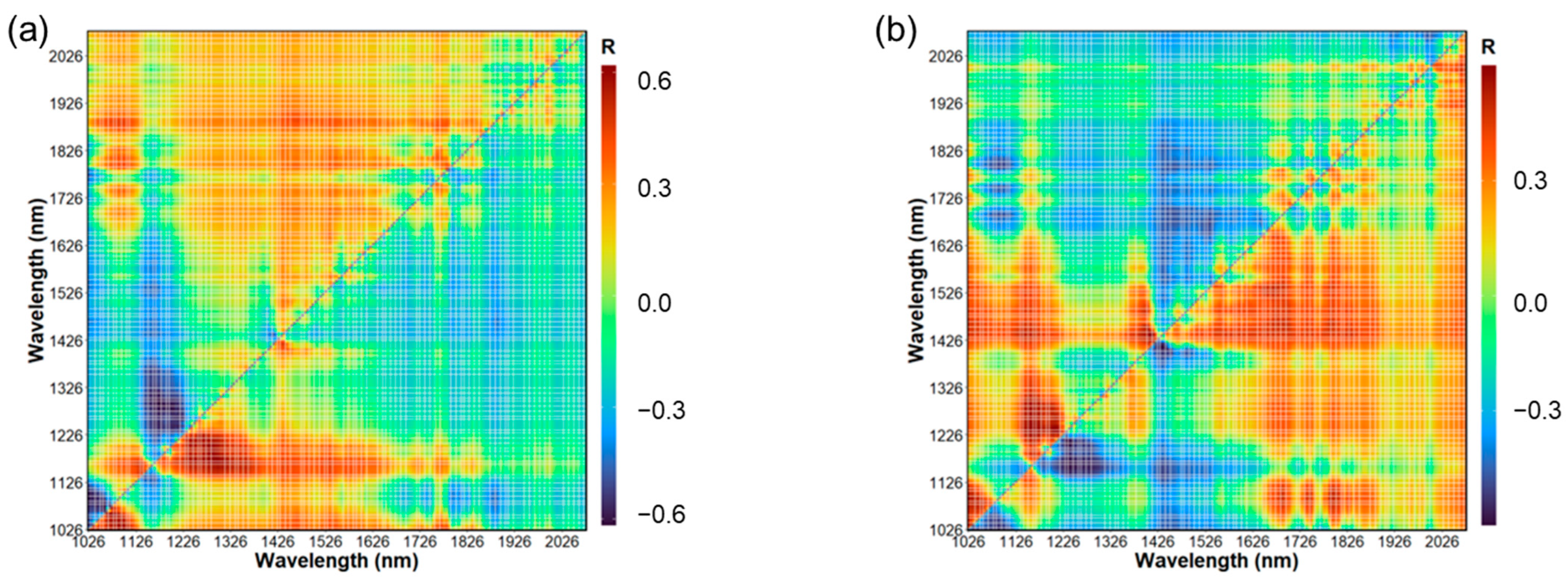
To minimize the signal noise and scattering effect, hyperspectral reflectance was transformed into narrowband spectral indices, such as the spectral ratio (SR), difference spectral indices (DSIs) and normalized difference spectral indices (NDSIs) [22]. Among them, the NDSI has been widely used, and thus we explored the correlation between the TSS, TA and NDSI, as shown in Figure 5. The NDSI was calculated for each possible wavelength combination. The highest correlation variable between the TSS and NDSI was (R1289 − R1177)/(R1289 + R1177), with a correlation coefficient of 0.62. In addition, (R1294 − R1177)/(R1294 + R1177), (R1076 − R1060)/(R1076 + R1060) and (R1300 − R1177)/(R1300 + R1177) had high correlation with the TSS. The most relevant NDSI with the TA was (R1411 − R1434)/(R1411 + R1434), with a correlation coefficient of 0.6. The correlation plots showed the combination of NDSIs between 1500–1800 nm had a higher correlation with the TA than the TSS (Figure 5).

3.3. Predictive Model Performance Based on Regression Models

The results obtained for testing the dataset based on different predictive models are shown in Table 3. Previous studies commonly used the RMSE and R2 to evaluate model performance, indicating that the best performance model shows low RMSE and high R2 values. In addition to the RMSE and R2, we used the RPD and CCC to evaluate the model performance. The RPD represents the ratio of a variable’s standard deviation to its standard error of prediction using a specific model. For the RPD, a model is considered almost perfect when RPD > 2, a moderate model when 2 > RPD > 1.4 and a poor model when RPD < 1.4 [23]. The CCC represents how close a model prediction conforms to the ground truth data along a 45 degree line from the origin. For the CCC, there is an excellent model with CCC > 0.8, a moderate model with 0.8 > CCC > 0.65 and a poor model with CCC < 0.65 [24].
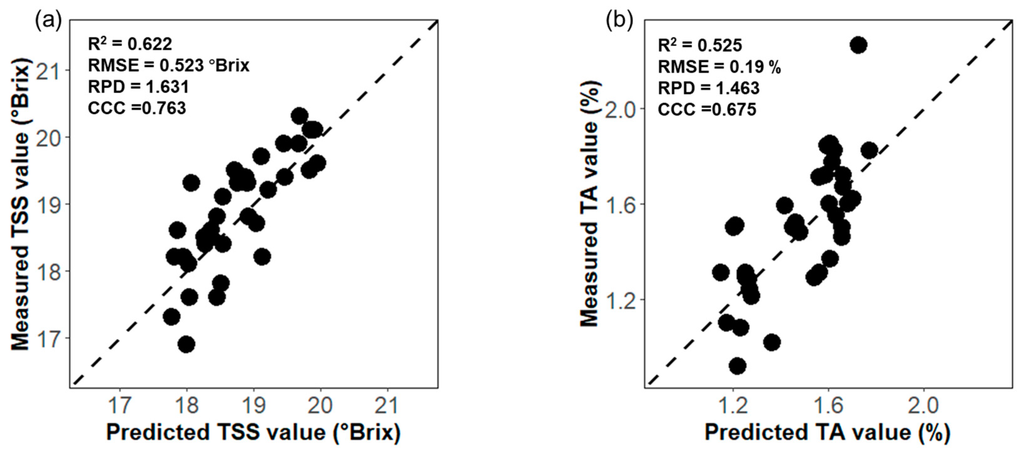
For predicting the TSS based on MSC+SG spectral preprocessing, the PLSR presented an RMSE, R2, RPD and CCC of 0.554 °Brix, 0.583, 1.54 and 0.693, respectively. The results of predicting the TSS based on NDSI spectral preprocessing were an RMSE of 0.726 °Brix, an R2 of 0.305, an RPD of 1.114 and a CCC of 0.548 in the PLSR model. When it came to the TA, the PLSR showed poor performance with both the MSC+SG and NDSI preprocessing methods (Table 3). The PLSR has been established as an effective predictive model for processing hyperspectral data [1,7,25]. In this study, the results show that the PLSR had moderate performance when predicting a grape’s TSS through using MSC+SG preprocessing, while it had poor performance when predicting the grape’s TA. In addition to traditional regression models, we also explored the predictive power of two machine learning models (SVR and RFR). For SVR, the results of predicting the TSS based on MSC+SG preprocessing showed the best prediction performance among all the regression models, with a resulting RMSE, R2, RPD and CCC of 0.523 °Brix, 0.622, 1.631 and 0.763, respectively. When using the selected NDSIs as the input variables, the prediction performance of the SVR model decreased but still showed moderate prediction performance (Table 3). For predicting the TA based on the MSC+SG preprocessing features, SVR presented poor model performance, with an RMSE, R2, RPD and CCC of 0.333%, 0.03, 0.751 and 0.168, respectively. The combination of SVR and NDSI preprocessing showed moderate prediction accuracy, with an RMSE, R2, RPD and CCC of 0.19%, 0.525, 1.463 and 0.675, respectively. For RFR, the results of predicting the TSS based on MSC+SG preprocessing showed poor model performance (RMSE = 0.642 °Brix, R2 = 0.449, RPD = 1.368 and CCC = 0.549). When the selected NDSIs were used as input variables, the performance of the RFR model was better than that using MSC+SG and showed moderate performance (Table 3). When using MSC+SG for the input variables, the RFR model showed the best model performance (RMSE = 0.217%, R2 = 0.43, RPD = 1.346 and CCC = 0.595) in predicting a grape’s TA compared with other regression models (Table 3). In addition, the combination of RFR and NDSIs showed moderate prediction performance to predict a grape’s TA (Table 3). Figure 6 shows the best model performance when predicting a grape’s TSS and TA.

3.4. Spectral Feature Importance of TSS and TA

In order to identify the spectral signatures that contributed the most to the model’s performance, the feature importance of the best performance model based on MSC+SG preprocessing was calculated (Figure 7). The PFI measures a feature’s importance by calculating the increase in the model’s prediction error after permuting the feature. For example, the reflectance value in band 1104 was most important for the SVR model predicting the TSS. If permuting the wavelength of 1104 nm in the data, then the RMSE of the SVR model increased by a factor of around 1.04. In addition, the PFI values show that the electromagnetic spectrum contributed more at approximately 1088–1127, 1278–1322 and 1810–1838 nm (Figure 7a). The PFI values for the RFR model predicting the TA fluctuated near 1088–1104, 1138–1155, 1227, 1250 and 1788 nm (Figure 7b). Figure 7 indicates that the PFI values were large at approximately 1100 nm in the TSS and TA prediction model. The peaks at 1100 nm were due to vibrations related to the O-H and C-H bonds [26]. It is worth noting that the NDSI values of the combination of these bands also had a high Pearson’s correlation coefficient with the TSS or TA. Therefore, future studies should continue to explore the potential of using these relevant narrowband NDSIs to classify or predict grape maturity.

3.5. Discrimination Capacity Based on Classification Models

Classification analyses were performed for fresh berries using LDA, SVMs and RFs. The samples were divided into two groups (high and low quality) for each parameter and separated by the threshold-limiting values: 19 °Brix for the TSS and 1.5% for the TA. Table 4 shows the discrimination capacity of grape quality using different classification models and spectral preprocessing methods. The LDA model of the TSS presented a moderate classification capacity, with an accuracy rate of 75% for the MSC+SG dataset and 68.8% for the NDSI dataset. When using SVMs to discriminate the TSS, 78.1% of the samples were correctly classified with MSC+SG features, and 93.8% of the samples were correctly classified with NDSI features. When using RFs to discriminate the TSS, the percentage of total samples correctly classified was 84.4% with MSC+SG features and 90.6% with NDSI features. With respect to the TA classification of fresh berries, the two quality groups were correctly classified with an accuracy rate from 75% to 84.4%. Compared with MSC+SG, NDSI preprocessing has the ability to improve the classification performance when discriminating grape quality parameters.

4. Discussion

The PLSR, SVR and RFR models developed based on an SWIR hyperspectral imaging system showed overall moderate performance for predicting the TSS. When comparing the present work to previous work carried out for reflectance models, for the TSS, the present R2 values were slightly worse than those in [1,8,27]. One possible reason for this is that the range of the spectrum used in the previous study was 400–1000 nm. However, when using the RMSE as the model performance criteria, the present work showed better performance than those in previous studies. We used the RPD and CCC to further assess the regression model’s performance. The results show that the combination of SVR and MSC+SG demonstrated moderate prediction performance (RPD = 1.631 and CCC = 0.763). The comparison suggests that the spectrum range between 400 and 1000 nm may be more informative for quantifying the TSS value of grape berries. This is because a VIS–NIR HSI system for predicting grape TSS values may be more practical, given that it is usually cheaper and has better predictive performance than an SWIR HSI system for industry use. In addition, using a different variety of grape than those in previous works may have contributed to the poor performance of our model. Compared with the TSS, the prediction for the TA was lower in the regression models. The model accuracy was also worse than in previous findings [14,28]. Previous studies mainly used HSI between 400 and 1000 nm to predict the TA. The authors of [14] used a portable spectrophotometer to measure the enological parameters in the spectral range of 400–1000 nm. An R2 of 0.81 was obtained for estimating a grape’s TA value in [14]. The reduced predictive accuracy compared with the present work may be due to the different regression models, spectroscopic modes and grape varieties. Future studies should continue to explore using current HSI systems to predict enological parameters based on different grape varieties. It is noticeable that this study used two spectra preprocessing methods: MSC+SG and NDSIs. The NDSI preprocessing method significantly improved the model prediction performance when predicting the TA value. Additionally, the smoothing techniques used in this study possibly filtered the noise of raw reflectance data through the rapid exposure time. However, a smoothing technique will lose some characteristic values when processing spectral data, and thus further studies should try to adjust the camera parameters to avoid using a smoothing technique.
This study also examined the possibility of using an HSI system to classify grape maturity. The SVM and RF models showed good classification performance for the TSS. Compared with the TSS, the LDA, SVM and RF models only showed moderate classification performance for the TA. The classification accuracies were higher than those om [14], where the combination of a spectrometer (1600–2400 nm) and PLS-DA was used to classify grape maturity, obtaining 77.1% for the TSS and 68.6% for the TA. However, the 84.4% accuracy rate when classifying the TA cannot meet the requirements for industrial application. The low sample size used in this study may have limited the classification model’s performance when classifying the TA. Thus, further studies can use larger sample sizes with a wide range of TA values to examine the classification model’s performance. When compared with a study using a spectrum of 350–2500 nm, our classification accuracy was similar to that in [12], where different supervised classification methods were used to determine the maturation stage of wine grapes, obtaining accuracy rates from 92.26 to 93.15%. However, it is worth noting that running HSI or spectrometers in the range of 400–2500 nm is expensive for industrial applications. Further research can continue to explore the possibility of selecting a specific band range for grading grape quality. In conclusion, classification models in this study would combine with current optical berry sorting systems to give winemakers a non-destructive tool for selecting the preferred berries.

5. Conclusions

The presented study explored the feasibility of applications of non-destructive means of estimating the TSS and TA values of wine grapes by using the SWIR, with hyperspectral imaging in the spectral range of 1000–2500 nm. The Pearson’s correlation coefficient between the NDSI, TSS and TA showed that the NDSIs (R1289 − R1177)/(R1289 + R1177) and (R1411 − R1434)/(R1411 + R1434) had high correlation with the TSS and TA, respectively. Furthermore, PLSR, SVR and RFR models were constructed to predict the TSS and TA based on the MSC+SG features or NDSI features. The prediction results demonstrate that the TSS of wine grapes can be predicted with moderate performance using SVR combined with an MSC+SG spectral pretreatment process (RMSE = 0.523 °Brix, R2 = 0.622, RPD = 1.631 and CCC = 0.763). Compared with the TSS, the regression model performance values for the TA were relatively low, with the best model performance obtained from SVR combined with NDSI preprocessing (RMSE = 0.19%, R2 = 0.525, RPD = 1.463 and CCC = 0.675). We explored the spectral feature importance of the TSS and TA, and the results indicate that the significant regions and wavelengths relevant to TSS and TA estimation were at around 1100 nm. Finally, LDA, SVM and RF models were used to discriminate a grape’s TSS and TA through different spectral preprocessing methods. Samples were divided into high or low quality for each parameter based on a threshold limiting value. The results show that the best model correctly classified 93.8% of the samples for distinguishing the TSS and 84.4% of the samples for distinguishing the TA. To enhance the industrial applicability of this technique, it is crucial to validate the developed regression or classification models on a broader range of wine grape varieties. This study has demonstrated the potential of using NIR-SWIR hyperspectral imaging for the rapid and non-destructive determination of the TSS and TA values of wine grapes.

Author Contributions

Conceptualization, H.L. and M.G.; methodology, H.L., T.R., M.G. and M.I.; software, H.L., M.I. and E.S.; validation, H.L., T.R., M.I. and E.S.; formal analysis, H.L.; investigation, H.L., E.S., T.R. and M.I.; resources, M.G. and E.S.; data curation, H.L., M.I. and E.S.; writing—original draft preparation, H.L.; writing—review and editing, M.G. and T.R.; visualization, H.L. and M.I.; supervision, M.G., T.R. and M.I.; project administration, M.G.; funding acquisition, M.G. All authors have read and agreed to the published version of the manuscript.

Funding

This research received no external funding.

Data Availability Statement

The raw data supporting the conclusions of this article will be made available by the authors on request.

Conflicts of Interest

The authors declare no conflict of interest.

Appendix A

Figure A1. Boxplot of TSS (a) and TA (b).
Remotesensing 16 01655 g0a1

References

  1. Gomes, V.; Fernandes, A.; Faia, A.; Melo-Pinto, P. Comparison of Different Approaches for the Prediction of Sugar Content in New Vintages of Whole Port Wine Grape Berries Using Hyperspectral Imaging. Comput. Electron. Agric. 2017, 140, 244–254. [Google Scholar] [CrossRef]
  2. Lee, J.-H.; Kang, T.H.; Um, B.H.; Sohn, E.-H.; Han, W.-C.; Ji, S.-H.; Jang, K.-H. Evaluation of Physicochemical Properties and Fermenting Qualities of Apple Wines Added with Medicinal Herbs. Food Sci. Biotechnol. 2013, 22, 1039–1046. [Google Scholar] [CrossRef]
  3. Baluja, J.; Tardaguila, J.; Ayestaran, B.; Diago, M.P. Spatial Variability of Grape Composition in a Tempranillo (Vitis Vinifera L.) Vineyard over a 3-Year Survey. Precis. Agric. 2013, 14, 40–58. [Google Scholar] [CrossRef]
  4. Bramley, R.; Pearse, B.; Chamberlain, P. Being Profitable Precisely -A Case Study of Precision Viticulture from Margaret River. Aust. New Zealand Grapegrow. Winemak. Annu. Tech. Issue 2003, 473a, 84–87. [Google Scholar]
  5. Zhao, M.; Cang, H.; Chen, H.; Zhang, C.; Yan, T.; Zhang, Y.; Gao, P.; Xu, W. Determination of Quality and Maturity of Processing Tomatoes Using Near-Infrared Hyperspectral Imaging with Interpretable Machine Learning Methods. LWT 2023, 183, 114861. [Google Scholar] [CrossRef]
  6. Li, S.; Luo, H.; Hu, M.; Zhang, M.; Feng, J.; Liu, Y.; Dong, Q.; Liu, B. Optical Non-Destructive Techniques for Small Berry Fruits: A Review. Artif. Intell. Agric. 2019, 2, 85–98. [Google Scholar] [CrossRef]
  7. Chen, S.; Zhang, F.; Ning, J.; Liu, X.; Zhang, Z.; Yang, S. Predicting the Anthocyanin Content of Wine Grapes by NIR Hyperspectral Imaging. Food Chem. 2015, 172, 788–793. [Google Scholar] [CrossRef]
  8. Silva, R.; Gomes, V.; Mendes-Faia, A.; Melo-Pinto, P. Using Support Vector Regression and Hyperspectral Imaging for the Prediction of Oenological Parameters on Different Vintages and Varieties of Wine Grape Berries. Remote Sens. 2018, 10, 312. [Google Scholar] [CrossRef]
  9. Ferrer-Gallego, R.; Hernández-Hierro, J.M.; Rivas-Gonzalo, J.C.; Escribano-Bailón, M.T. Determination of Phenolic Compounds of Grape Skins during Ripening by NIR Spectroscopy. LWT-Food Sci. Technol. 2011, 44, 847–853. [Google Scholar] [CrossRef]
  10. González-Caballero, V.; Sánchez, M.-T.; Fernández-Novales, J.; López, M.-I.; Pérez-Marín, D. On-Vine Monitoring of Grape Ripening Using near-Infrared Spectroscopy. Food Anal. Methods 2012, 5, 1377–1385. [Google Scholar] [CrossRef]
  11. Urraca, R.; Sanz-Garcia, A.; Tardaguila, J.; Diago, M.P. Estimation of Total Soluble Solids in Grape Berries Using a Hand-held NIR Spectrometer under Field Conditions. J. Sci. Food Agric. 2016, 96, 3007–3016. [Google Scholar] [CrossRef]
  12. dos Santos Costa, D.; Mesa, N.F.O.; Freire, M.S.; Ramos, R.P.; Mederos, B.J.T. Development of Predictive Models for Quality and Maturation Stage Attributes of Wine Grapes Using Vis-Nir Reflectance Spectroscopy. Postharvest Biol. Technol. 2019, 150, 166–178. [Google Scholar] [CrossRef]
  13. Dambergs, R.G.; Cozzolino, D.; Esler, M.B. The Use of near Infrared Spectroscopy for Rape Quality Measurement. Aust. New Zealand Grapegrow. Winemak. 2003, 69–76. [Google Scholar]
  14. Guidetti, R.; Beghi, R.; Bodria, L. Evaluation of Grape Quality Parameters by a Simple Vis/NIR System. Trans. ASABE 2010, 53, 477–484. [Google Scholar] [CrossRef]
  15. Wei, H.-E.; Grafton, M.; Bretherton, M.; Irwin, M.; Sandoval, E. Evaluation of Point Hyperspectral Reflectance and Multivariate Regression Models for Grapevine Water Status Estimation. Remote Sens. 2021, 13, 3198. [Google Scholar] [CrossRef]
  16. Lyu, H.; Grafton, M.; Ramilan, T.; Irwin, M.; Sandoval, E. Assessing the Leaf Blade Nutrient Status of Pinot Noir Using Hyperspectral Reflectance and Machine Learning Models. Remote Sens. 2023, 15, 1497. [Google Scholar] [CrossRef]
  17. Lyu, H.; Grafton, M.; Ramilan, T.; Irwin, M.; Wei, H.-E.; Sandoval, E. Using Remote and Proximal Sensing Data and Vine Vigor Parameters for Non-Destructive and Rapid Prediction of Grape Quality. Remote Sens. 2023, 15, 5412. [Google Scholar] [CrossRef]
  18. Pullanagari, R.R.; Li, M. Uncertainty Assessment for Firmness and Total Soluble Solids of Sweet Cherries Using Hyperspectral Imaging and Multivariate Statistics. J. Food Eng. 2021, 289, 110177. [Google Scholar] [CrossRef]
  19. Williams, P.; Norris, K. Near-Infrared Technology in the Agricultural and Food Industries; American Association of Cereal Chemists, Inc.: St Paul, MN, USA, 1987; ISBN 0-913250-49-X. [Google Scholar]
  20. Iqbal, A.; Sun, D.-W.; Allen, P. Prediction of Moisture, Color and pH in Cooked, Pre-Sliced Turkey Hams by NIR Hyperspectral Imaging System. J. Food Eng. 2013, 117, 42–51. [Google Scholar] [CrossRef]
  21. Fairuz Omar, A. Spectroscopic Profiling of Soluble Solids Content and Acidity of Intact Grape, Lime, and Star Fruit. Sens. Rev. 2013, 33, 238–245. [Google Scholar] [CrossRef]
  22. Wang, F.; Zhao, C.; Yang, H.; Jiang, H.; Li, L.; Yang, G. Non-Destructive and in-Site Estimation of Apple Quality and Maturity by Hyperspectral Imaging. Comput. Electron. Agric. 2022, 195, 106843. [Google Scholar] [CrossRef]
  23. Chang, C.-W.; Laird, D.A.; Mausbach, M.J.; Hurburgh, C.R. Near-infrared Reflectance Spectroscopy–Principal Components Regression Analyses of Soil Properties. Soil Sci. Soc. Am. J. 2001, 65, 480–490. [Google Scholar] [CrossRef]
  24. Zhao, X.; Zhao, D.; Wang, J.; Triantafilis, J. Soil Organic Carbon (SOC) Prediction in Australian Sugarcane Fields Using Vis–NIR Spectroscopy with Different Model Setting Approaches. Geoderma Reg. 2022, 30, e00566. [Google Scholar] [CrossRef]
  25. Grafton, M.; Kaul, T.; Palmer, A.; Bishop, P.; White, M. Regression Analysis of Proximal Hyperspectral Data to Predict Soil pH and Olsen P. Agriculture 2019, 9, 55. [Google Scholar] [CrossRef]
  26. Golic, M.; Walsh, K.; Lawson, P. Short-Wavelength near-Infrared Spectra of Sucrose, Glucose, and Fructose with Respect to Sugar Concentration and Temperature. Appl. Spectrosc. 2003, 57, 139–145. [Google Scholar] [CrossRef]
  27. Gutiérrez, S.; Tardáguila, J.; Fernández-Novales, J.; Diago, M.P. On-the-go Hyperspectral Imaging for the In-field Estimation of Grape Berry Soluble Solids and Anthocyanin Concentration. Aust. J. Grape Wine Res. 2019, 25, 127–133. [Google Scholar] [CrossRef]
  28. González-Caballero, V.; Pérez-Marín, D.; López, M.-I.; Sánchez, M.-T. Optimization of NIR Spectral Data Management for Quality Control of Grape Bunches during On-Vine Ripening. Sensors 2011, 11, 6109–6124. [Google Scholar] [CrossRef]
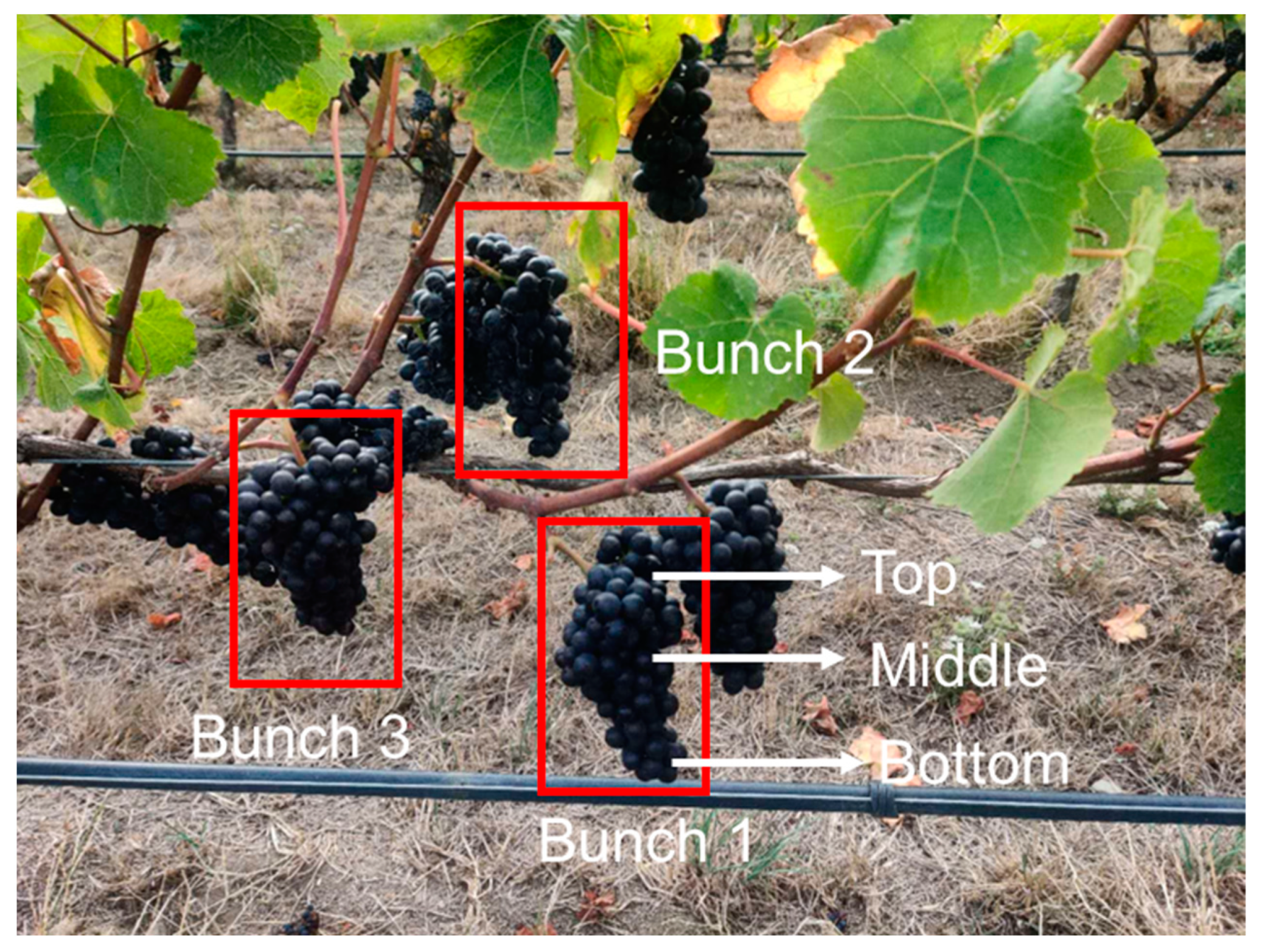
Figure 1. Example of the sampled grapevine.
Remotesensing 16 01655 g001
Figure 2. The Specim SWIR hyperspectral imaging system.
Remotesensing 16 01655 g002
Figure 3. The sampled grape berries image in the 1177 nm band (a) and region of interest grape berries (b).
Remotesensing 16 01655 g003
Figure 4. Reflectance spectrum of pinot noir variety.
Remotesensing 16 01655 g004
Figure 5. Correlation coefficient between NDSI and TSS (a) and TA (b).
Remotesensing 16 01655 g005
Figure 6. Predicted vs. measured values of TSS of grapes using SVR and MSC+SG (a). Predicted vs. measured values of TA of grapes using SVR and NDSI (b). The dotted line is the 1:1 line.
Remotesensing 16 01655 g006
Figure 7. The permutation feature importance for the TSS based on the SVR model (a) and the TA based on the RFR model (b).
Remotesensing 16 01655 g007
Table 1. The number of samples during each sampling date.
DateNumber of Samples
7 March22
15 March57
27 March33
Table 2. Descriptive statistics of enological parameters during study period.
ParameterDateNMinimumMaximumMeanSD
°Brix7 March2117.31918.210.58
15 March5316.919.918.630.67
27 March3318.821.219.590.49
TA7 March211.282.261.720.33
15 March531.171.931.590.17
27 March330.921.511.230.14
N = number of samples; SD = standard deviation.
Table 3. Model performance on testing set based on regression models.
ParameterFeatureModelRMSERPDR2CCC
TSS (°Brix)MSC+SGPLSR0.5541.540.5830.693
MSC+SGSVR0.5231.6310.6220.763
MSC+SGRFR0.6421.3680.4490.549
NDSIPLSR0.7261.1140.3050.548
NDSISVR0.5431.490.5890.655
NDSIRFR0.5921.4290.5310.687
TA (%)MSC+SGPLSR0.3050.820.0250.15
MSC+SGSVR0.3330.7510.030.168
MSC+SGRFR0.2171.3460.430.595
NDSIPLSR0.2071.3430.510.54
NDSISVR0.191.4630.5250.675
NDSIRFR0.1981.4440.50.652
Table 4. Discrimination performance on the testing set based on classification models.
ParameterFeatureModelAccFPRecallCe
TSS (°Brix)MSC+SGLDA0.7510.5880.25
MSC+SGSVM0.78150.8460.219
MSC+SGRF0.84420.80.156
NDSILDA0.68870.7690.313
NDSISVM0.93810.9330.0625
NDSIRF0.90620.9330.094
TA (%)MSC+SGLDA0.7570.9330.25
MSC+SGSVM0.78110.6670.219
MSC+SGRF0.84420.80.156
NDSILDA0.7570.9410.25
NDSISVM0.84430.8570.156
NDSIRF0.84430.8570.156
Disclaimer/Publisher’s Note: The statements, opinions and data contained in all publications are solely those of the individual author(s) and contributor(s) and not of MDPI and/or the editor(s). MDPI and/or the editor(s) disclaim responsibility for any injury to people or property resulting from any ideas, methods, instructions or products referred to in the content.