Article

Refined Analysis of Vegetation Phenology Changes and Driving Forces in High Latitude Altitude Regions of the Northern Hemisphere: Insights from High Temporal Resolution MODIS Products

1
State Key Laboratory of Resources and Environment Information System, Institute of Geographic Sciences and Natural Resources Research, Chinese Academy of Sciences, Beijing 100101, China
2
Peng Cheng Laboratory, Shenzhen 518000, China
3
State Key Laboratory of Desert and Oasis Ecology, Xinjiang Institute of Ecology and Geography, Chinese Academy of Sciences, Urumqi 830011, China
4
Key Laboratory of Low Altitude Geographic Information and Air Route, Civil Aviation Administration of China, Beijing 100101, China
5
The Research Center for UAV Applications and Regulation, Chinese Academy of Sciences, Beijing 100101, China
6
Faculty of Geographical Science, Beijing Normal University, Beijing 100875, China
7
University of the Chinese Academy of Sciences, Beijing 100049, China
8
Xinjiang Key Laboratory of Water Cycle and Utilization in Arid Zone, Urumqi 830011, China
*
Author to whom correspondence should be addressed.
These authors contributed equally to this work.
Remote Sens. 2024, 16(10), 1744; https://doi.org/10.3390/rs16101744
Submission received: 14 March 2024 / Revised: 4 May 2024 / Accepted: 11 May 2024 / Published: 14 May 2024

Abstract

:
The vegetation patterns in high-latitude and high-altitude regions (HLAR) of the Northern Hemisphere are undergoing significant changes due to the combined effects of global warming and human activities, leading to increased uncertainties in vegetation phenological assessment. However, previous studies on vegetation phenological changes often relied on long-term time series of remote sensing products for evaluation and lacked comprehensive analysis of driving factors. In this study, we utilized high temporal resolution seamless MODIS products (MODIS-NDVISDC and MODIS-EVI2SDC) to assess the vegetation phenological changes in High-Latitude-Altitude Regions (HLAR) of the Northern Hemisphere. We quantified the differences in vegetation phenology among different land-use types and determined the main driving factors behind vegetation phenological changes. The results showed that the length of the growing season (LOS) derived from MODIS-NDVISDC was 8.9 days longer than that derived from MODIS-EVI2SDC, with an earlier start of the growing season (SOS) by 1.5 days and a later end of the growing season (EOS) by 7.4 days. Among different vegetation types, deciduous needleleaf forests exhibited the fastest LOS extension (p < 0.01), while croplands showed the fastest LOS reduction (p < 0.05). Regarding land-use transitions, the conversion of built-up land to forest and grassland had the longest LOS. In expanding agricultural areas, the LOS of land converted from built-up land to cropland was significantly higher than that of other land conversions. We analyzed human activities and found that as the human footprint gradient increased, the LOS showed a decreasing trend. Among the climate-related factors, the dominant response of phenology to temperature was the strongest in the vegetation greening period. During the vegetation browning period, the temperature control was weakened, and the control of radiation and precipitation was enhanced, accounting for 20–30% of the area, respectively. Finally, we supplement and prove that the highest contributions to vegetation greening in the Northern Hemisphere occurred during the SOS period (May–June) and the EOS period (October). Our study provides a theoretical basis for vegetation phenological assessment under global change. It also offers new insights for land resource management and planning in high-latitude and high-altitude regions.

Graphical Abstract

1. Introduction

One strategy for land vegetation to adapt to environmental changes to continuously adjust its growth and development patterns, including early greening and delayed dormancy [1,2,3]. Climate change, including increasing temperatures [4], changing precipitation patterns [5], solar radiation [6], wind speed [7], and environmental factors such as carbon dioxide (CO2) and atmospheric nitrogen (N) deposition [8], is a major factor leading to changes in vegetation phenology, such as budburst, leaf expansion, flowering, fruiting, and leaf senescence. However, in addition to climate change, the impact of land use and land cover change (LULCC) on vegetation phenology in high-latitude regions is often overlooked. Human activities, through changes in land use and management practices, alter surface vegetation patterns and structures, which also have significant impacts on ecosystem services and biodiversity [9]. The impact of LULCC on vegetation phenology is manifested in changes in vegetation types or as feedback after greening. Furthermore, LULCC can also affect ecological processes such as ecosystem structure and function, carbon balance [10], water cycle, and energy flow [11,12]. While the greening of the land’s surface has contributed to carbon sinks in the past two decades [9,13], it can also have negative impacts on the surrounding environment, leading to a reduction in ecosystem services. For example, increased transpiration resulting from greening can lead to soil moisture deficits, increasing the frequency of drought events in water-limited arid and semi-arid regions [14]. This can disrupt the natural phenological cycles of plants and affect their growth and development patterns. Therefore, it is important to understand the impact of vegetation dynamics and patterns on phenology.
Remote sensing-based land surface phenology (LSP) refers to the phenological information of land surface reflectance captured at the pixel scale by satellite sensors [15,16]. Currently, a significant amount of research focuses on overall studies of different vegetation functional types, neglecting the phenology of native functional types and the LSP differences caused by LULCC [17,18,19]. For example, native vegetation exhibits a higher resistance to environmental disturbances due to its stable ecological community structure compared to non-native vegetation [20,21]. Non-native vegetation may require more or less water and soil nutrients during its growth compared to native vegetation [14,22,23], and it also shows different responses to climate compared to native vegetation during environmental adaptation [19]. Therefore, it is of great significance to elucidate the phenological differences among different vegetation types and under LULCC in order to gain a deep understanding of the driving mechanisms of regional vegetation phenology.
Currently, most remote sensing datasets used to retrieve LSP, such as MODIS products (MOD13Q1, MOD13A2, MOD09A1) with 16-day or 8-day intervals and the AVHRR GIMMS NDVI3g dataset with a 15-day interval, are generated using the maximum value synthesis method. These products excel at mitigating cloud/shadow effects and reducing noise in surface bidirectional reflectance [24,25,26,27]. However, there is considerable uncertainty in the accuracy of LSP using the maximum value synthesis method. Some studies have quantified the influence of temporal resolution differences on the accuracy of phenological retrieval, emphasizing the importance of temporal resolution [28,29,30]. Other studies have indicated that higher temporal resolution leads to higher accuracy in phenological retrieval [31,32,33]. Therefore, selecting datasets with the highest possible temporal resolution is crucial for improving the accuracy of LSP retrieval.
The human footprint integrates various pressure indicators, including the built environment, nighttime lights, population density, land cover, and land use changes, to comprehensively assess the degree of environmental impact caused by human activities [34]. Compared to single indicators, the human footprint provides a better understanding of the extent to which human activities affect the natural environment and has been widely applied in studies evaluating the impact of human activities on biodiversity conservation and climate change [35,36,37]. Previous research has utilized the human footprint to assess the differential trends in NDVI and LST (Land Surface Temperature) based on the MCD43C4 (Collection5 and Collection6) and MOD11C2 (Collection5 and Collection6) datasets [38]. The human footprint serves as an important indicator for assessing the intensity of human activities and has been found to exert a moderate indirect negative influence on net primary productivity in the Qilian Mountain region [39]. Moreover, the human footprint has been utilized to calculate the ecological vulnerability index for the Qinghai-Tibet Plateau region and quantify important indicators of vegetation-driven impacts in ecologically fragile areas [40,41]. These studies highlight the potential of the human footprint in evaluating the impact of human activities on the natural environment, thus emphasizing the significance of research on vegetation phenology changes.
The HLAR in the Northern Hemisphere is known to be sensitive to climate responses [42,43]. Since the beginning of the 21st century, these regions have experienced significant climate changes and the combined effects of human activities. This study conducted a comparative analysis of phenological differences in the HLAR using the seamless data cube (SDC) product derived from MODIS data. The main objectives of this research were: (1) to quantitatively analyze the spatiotemporal variations of LSP in the HLAR using NDVISDC and EVI2SDC products; (2) to examine the differences in LSP across different land use changes in the HLAR; (3) to quantify the effects of human activities and climate factors on LSP in the HLAR; and (4) to analyze the response of LSP in the HLAR to global greening/browning. This study aims to provide a theoretical basis for assessing LSP in the HLAR under global change and to offer new insights for land resource management and planning in this region.

2. Materials and Methods

2.1. Study Area

The study area includes the continents of Eurasia and North America (Figure 1), with a total area of approximately 92.51 × 10⁶ km2. The dominant vegetation cover types in the area are grassland (46.25%), followed by other land uses (15.34%), forests (13.49%), shrubs (12.46%), croplands (8.15%), water bodies (3.97%), and built-up areas (0.34%). The region exhibits a diverse range of climate types, including temperate monsoon climate, temperate maritime climate, mediterranean climate, temperate continental climate, subarctic coniferous forest climate, plateau mountain climate, and frigid climate. In terms of topography, the study area includes the Qinghai-Tibet Plateau, which has some of the highest elevations in the world. Plains below 200 m in elevation account for 34.3% of the total area. The climate of the study area is characterized by an average temperature of −19.05 °C in January, an average temperature of 14.2 °C in July, and an average annual precipitation of 40.15 mm. The vegetation in the study area exhibits distinct latitudinal, longitudinal, and vertical zoning patterns [44].

2.2. Data Sources

2.2.1. Remote Sensing Dataset

The MODIS Seamless Data Cube (SDC) used in this study is obtained from the Pengcheng Star Cloud platform (http://data.starcloud.pcl.ac.cn/resource/28, accessed on 1 May 2024). This dataset is based on the daily MOD09GA 500m product and utilizes time-series algorithms to fill in gaps in discrete observations, effectively preserving the dynamic changes in surface reflectance [45]. The SDC product provides two spatial resolutions: 500 m and 0.05°. The 0.05° resolution is derived by aggregating data from the 500-m scale using the same method as MODIS’ aggregation from 500 m to 0.05°. Considering various factors, including data volume and temporal resolution, we have chosen the SDC reflectance dataset with a temporal interval of 4 days and a spatial resolution of 0.05° for conducting phenological research. This high-precision dataset provides the necessary conditions for accurately assessing vegetation phenology in the study area.
The land cover dataset chosen is MCD12C1 (https://lpdaac.usgs.gov/, accessed on 1 May 2024), which has been further aggregated into categories of forest, shrub, grassland, cropland, built-up land, water bodies, and other land using the International Geosphere-Biosphere Programme (IGBP) classification system. The dataset has a resolution of 0.05°. We have chosen the land cover datasets for the years 2001 and 2022 to calculate the land transfer matrix and conduct further research.

2.2.2. Climate Dataset

This study investigates the response of LSP to global climate change during the period from 2001 to 2022 using climate variables. The monthly precipitation and solar radiation datasets are sourced from the TerraClimate dataset (http://www.climatologylab.org/terraclimate.html, accessed on 1 May 2024) at a spatial resolution of approximately 4.6 km. The monthly temperature dataset is obtained from the MODIS MOD11C3 product (https://lpdaac.usgs.gov/, accessed on 1 May 2024), with a resolution of 0.05°. To maintain consistency in spatial resolution, the precipitation and solar radiation datasets were resampled to 0.05°.

2.2.3. Human Footprint Dataset

The human footprint dataset characterizes the degree of human pressure on the natural environment. A higher value indicates a greater level of disturbance caused by human activities in a specific area, while a lower value signifies a lesser impact from human activities [34]. For this study, we utilized the human footprint dataset from 2001 to 2020 (https://doi.org/10.6084/m9.figshare.16571064, accessed on 1 May 2024). The dataset has a spatial resolution of 1 km. Subsequently, the dataset was resampled to a resolution of 0.05°. To better analyze the influence of human activities on regional vegetation phenology, we categorized the dataset into five levels: lowest (0 < Value ≤ 10), low (10 < Value ≤ 20), medium (20 < Value ≤ 30), high (30 < Value ≤ 40), and highest (40 < Value ≤ 50).

2.2.4. Phenology Validation Dataset

The USA National Phenology Network (USA-NPN) has recorded a significant number of phenological events for deciduous forests (deciduous broadleaf forests and deciduous needleleaf forests) during spring and fewer events during autumn (https://www.usanpn.org/data#Dashboard, accessed on 1 May 2024). To ensure the accuracy of phenological observations, we compared the vegetation types associated with USA-NPN sites to the MCD12C1 land cover types. Sites with matching vegetation types were retained, while sites with unmatched vegetation types were not considered within the scope of validation.
Additionally, the observation dates were restricted to a range of 1–180 days for spring phenological events and 180–365 days for autumn phenological events. During the validation process, the SOS corresponded to breaking leaf buds phenophases in deciduous forests, while the MidGreendown corresponded to all leaves fallen phenophases in deciduous broadleaf forests and deciduous needleleaf forests [25,46]. Ultimately, 300 records of breaking leaf buds phenophases and 100 records of all leaves fallen phenophases for deciduous forests from 2011 to 2022 were selected for phenological validation.
The Pan-European Phenology Project (PEP27) records long-term phenological observations for 78 species in 25 European countries (http://www.pep725.eu/, accessed on 1 May 2024) [47]. Similarly, we matched the vegetation types associated with monitoring sites to the MCD12C1 land cover types and excluded sites with inconsistent vegetation types. In cases where multiple vegetation types were present at a site, the arithmetic mean was selected as the final phenological result for that site. The timing of SOS corresponds to the timing of the first visible leaves (BBCH11) in deciduous broadleaf forests and the first leaves separated (BBCH10) in evergreen needleleaf forests. The timing of MidGreendown corresponds to the date when leaves in deciduous broadleaf forests exhibit 50% autumn coloration (BBCH94) [48,49,50,51,52]. Due to the lack of autumn phenology data for evergreen needleleaf forests and grasslands, their autumn phenological stages were not considered in this study. Finally, 300 records of the first visible leaves and 50% autumn coloration dates for deciduous forests, as well as 73 records of the first leaves separated phenophase for evergreen needleleaf forests, were selected for phenological validation.

2.3. Methods

2.3.1. Retrieval of LSP

In HLAR of the Northern Hemisphere, the presence of snow-covered vegetation greatly affects the data quality of satellite observations and has significant implications for phenological retrieval. To mitigate the impact of snow on vegetation indices, previous studies have relied on either daily temperature data or the interpolation of monthly temperature data to a daily scale [53]. Subsequently, consecutive 5-day periods with temperatures below 0 °C are identified as snow pixels and replaced with values from the nearest uncontaminated dates [3,54]. However, the interpolation of monthly temperature data to a daily scale may introduce uncertainties. Additionally, in HLAR, where temperatures fluctuate greatly, using 0 °C as the threshold for determining the presence of snow may lead to misclassifying snow-free areas as snow-covered, further increasing the level of uncertainty. Therefore, considering the uncertainties associated with previous studies, we utilized spectral indices for snow identification. The Normalized Difference Snow Index (NDSI) was employed, where pixel values greater than 0 indicate the presence of snow in a particular area [55]. This method is also used by NASA for phenological datasets. In our study, we first calculated NDVI, EVI2, and NDSI using the SDC reflectance dataset (Table 1). Then, we filtered out snow using NDSI values greater than 0. Background values were replaced with the 5th percentile of non-snow observations. Finally, a Savitzky-Golay filter was applied to the data to smooth it and eliminate inherent noise.
The amplitude threshold method is used for phenological extraction, which is also utilized by NASA to generate phenology products. This method, originally proposed by Fischer [56], is applied using the NDVI from the SDC reflectance dataset (see Table S1 for details). Following the same procedure, seven phenological parameters are extracted: SOS, MidGreenup, Maturity, Senescence, MidGreendown, EOS, and LOS.
Table 1. Spectral index formulas.
Vegetation IndicesFormulasReferences
NDVI N D V I = P 2 P 1 / P 2 + P 1 [57]
EVI2 E V I 2 = 2.5 × P 2 P 1 / P 2 + 2.4 × P 1 + 1 [58]
NDSI N D S I = P 4 P 5 / P 4 + P 5 [59]
Note: P 1 represents the red band, P 2 represents the near-infrared band, P 4 represents the green band, and P 5 represents the shortwave infrared band.

2.3.2. Accuracy Assessment of LSP

We employed ordinary least squares linear regression models to establish the relationship between actual phenological observation and remote sensing vegetation index retrieval phenology. To evaluate the accuracy of vegetation index retrieval phenology, we utilized regression measurement statistics, including root mean square error (RMSE), R-squared (R2), and bias [60,61,62]. The smaller RMSE and bias indicate that the phenology retrieved by the remote sensing vegetation index is closer to the actual observed phenology, while the larger R2 indicates that the model has stronger explanatory power, that is, the use of the remote sensing vegetation index can better reflect phenological changes. The formula is as follows:
R M S E = 1 n i = 1 n y i ^ y i 2
R 2 = 1 i = 1 n y i y i ^ 2 i = 1 n y i y ¯ 2
B i a s = 1 n i = 1 n y i ^ y i
where y i ^ represents the phenological results obtained from remote sensing vegetation index retrievals, y i represents the corresponding actual observed results from the site, n represents the sample size, and y ¯ denotes the average value of the observed results.

2.3.3. Trend Detection Method

The spatial trend analysis of vegetation phenology applied the Theil-Sen slope estimation method [63]. When the slope is greater than 0, it indicates that the vegetation phenology is delayed, and when the slope is less than 0, it indicates that the vegetation phenology is advanced. At the same time, the Mann-Kendall test is used to measure the significance of the trend [64]. When the P value is less than 0.05, it shows that there is a significant trend in the results. These two methods have been widely used to detect phenological trend changes due to their high computational efficiency and no interference from spillover values [27,39,65,66]. The formula for Theil-Sen slope estimation can be written as follows:
S l o p e = M e d i u m x i x j i j
In the equation, S l o p e represents the trend change of vegetation phenological parameters estimated by Sen’s slope estimation method. x i and x j denote the values of the vegetation phenological parameters for the i -th and j -th years, respectively.

2.3.4. The Speed of Vegetation Development

In order to reveal the speed of vegetation development during each phenophase, Piao’s method was employed [67]. Taking the NDVI as an example, the calculation formula is as follows:
V N D V I t = N D V I t N D V I t 1
The V N D V I t represents the difference in NDVI between two consecutive months within the year. If V N D V I ( t ) > 0, it indicates the development of vegetation, while if V N D V I ( t ) < 0, it represents the senescence of the vegetation.

2.3.5. Partial Correlation Analysis

In this study, the partial correlation analysis method was used to investigate the correlations between precipitation, temperature, solar radiation, and LSP. Partial correlation refers to examining the correlation between a single climate factor and LSP while controlling for the influence of other climate factors [3]. The formula is as follows:
R x y × z = R x y R x z R y z 1 R x z 2 1 R y z 2
R x y denotes the correlation between x and y while controlling for z . R x y , R x z , and R y z represent the correlations between two factors. Due to the lagged and cumulative effects of climate on LSP, this study also investigated the optimal preseason length for each climate factor [42,68]. The preseason length was set from 0 to 4 months, and the maximum preseason partial correlation coefficient was used as the correlation between LSP and climate factors [69].

3. Results

3.1. Accuracy Verification of LSP

Based on the phenological results of deciduous vegetation recorded by the PEP27, they show good agreement with phenological observations obtained from remote sensing data (Figure 2). For PEP27, the timing of the first visible leaves in deciduous broadleaf forests (DBF) was concentrated between 60 and 110 days. The SOS derived from NDVISDC was concentrated between 40 and 120 days (R2 = 0.64, RMSE = 16.05 d). The SOS derived from EVI2SDC was concentrated between 65 and 115 days (R2 = 0.68, RMSE = 9.36 d). The timing of 50% of leaves exhibiting autumn coloration in deciduous broadleaf forests was concentrated between 250 and 310 days. The MidGreendown of NDVISDC was concentrated between 260–320 days (R2 = 0.62, RMSE = 12.39 d), while the MidGreendown of EVI2SDC was concentrated between 260–310 days (R2 = 0.65, RMSE = 6.81 d). Furthermore, the validation results of vegetation phenology derived from remote sensing observations exhibit high R2 and low RMSE when compared to the phenological records of evergreen forest from the PEP27 and deciduous forest observations from the USA-NPN (Table S2, Figures S1 and S2). Based on these findings, both vegetation indices provide acceptable accuracy in representing vegetation phenology results, thereby enabling further analysis and research.

3.2. Human Footprint and Land Use Changes in HLAR

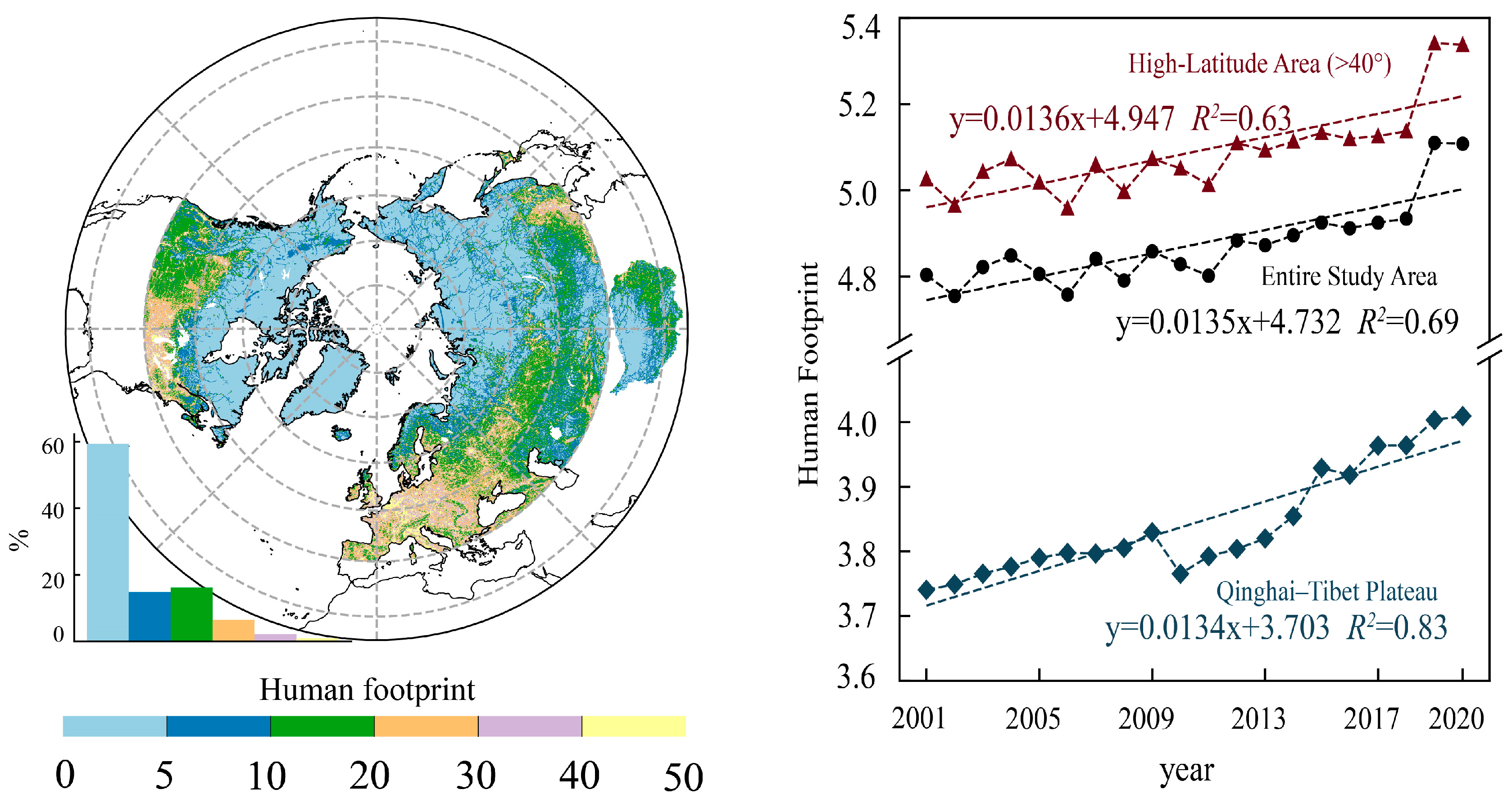
In the HLAR, the human footprint exhibits an overall increasing trend (+0.0135 yr−1), indicating a significant rise in the pressure exerted by human activities on the natural environment (Figure 3). The highest human footprint is observed in Europe and the Great Lakes region of North America, while the Arctic region has the lowest human footprint. From 2001 to 2022, the area of grassland experienced the largest increase, expanding by approximately 165.6 × 10⁴ km2, followed by built-up areas with an increase of approximately 2200 km2. Forests, shrubs, croplands, other land types, and water bodies all experienced decreases, with water bodies undergoing the largest reduction, amounting to a decrease of 84.61 × 10⁴ km2 (Table 2). The land transfer flow chart (Figure S3) reveals a predominant transition of land cover types towards grasslands, followed by forests.

3.3. Spatial and Temporal Variation of LSP

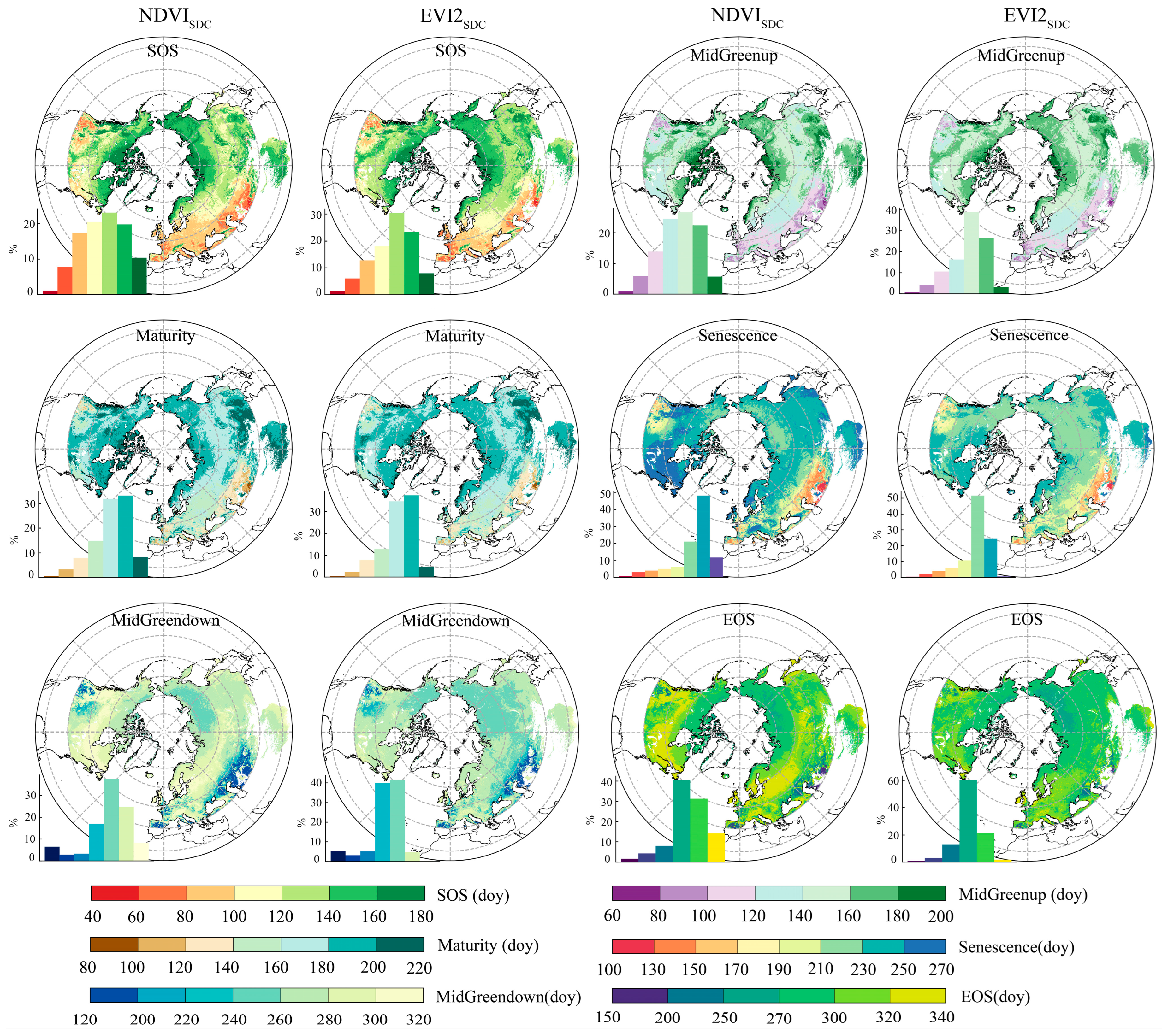
In the spatial distribution of LSP in HLAR (Figure 4), the general patterns of LSP of the two vegetation indices are similar. However, the difference between the two vegetation indices is still noticeable, the EVI2SDC shows a later date for vegetation greening compared to the NDVISDC (later days: 1.5 d for SOS, 2.9 d for MidGreenup, 0.1 d for Maturity). Additionally, the vegetation senescence phase of EVI2SDC occurs earlier than NDVISDC (earlier days: 9.2 d for Senescence, 11.5 d for MidGreendown, 7.4 d for EOS). The LOS of NDVISDC is longer than that of EVI2SDC (longer days: 8.9 d for LOS).
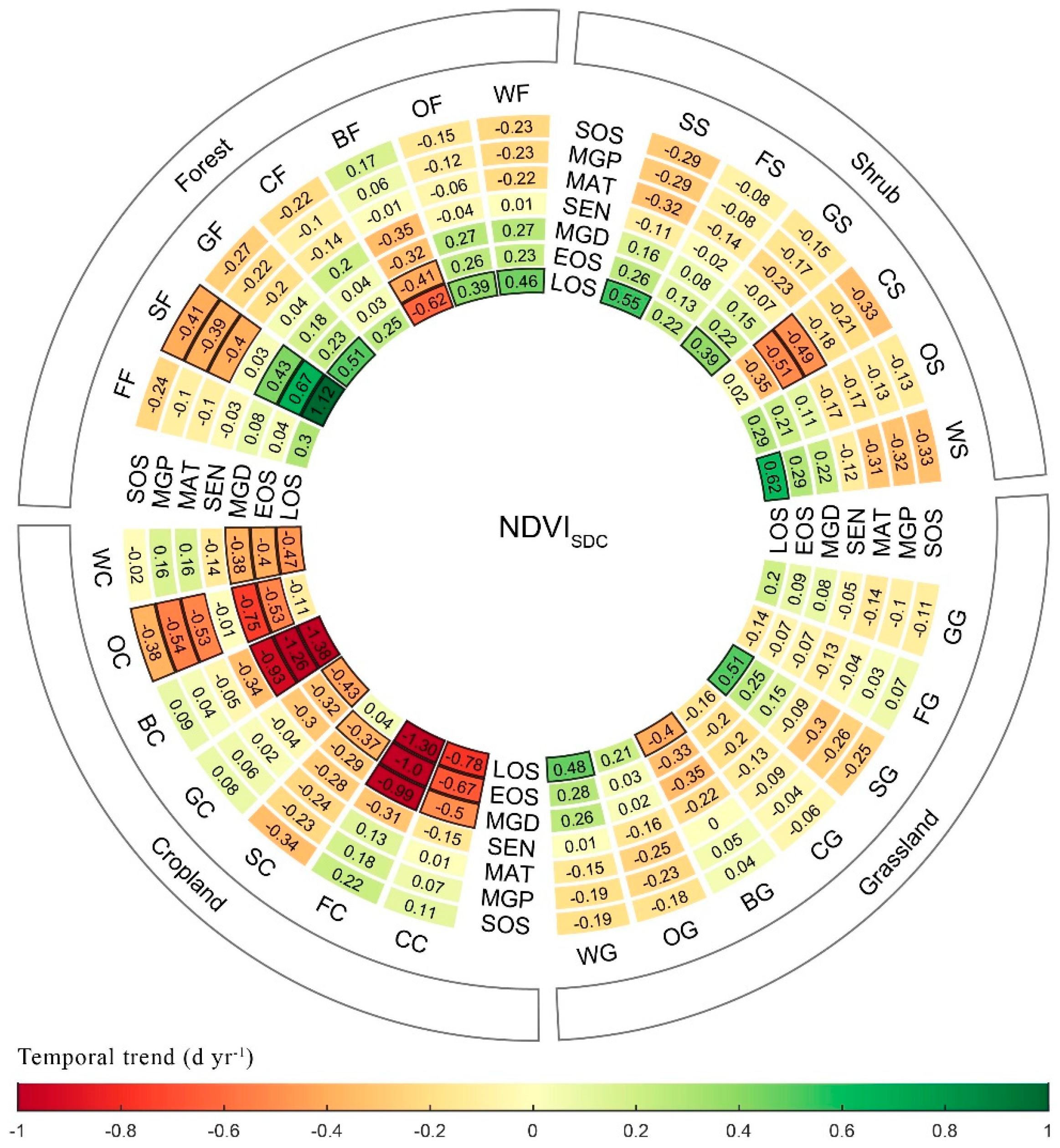
The LSP retrieved by NDVISDC and EVI2SDC showed no significant difference in the trend change (Figure 5). The trend of the SOS, MidGreenup, Maturity, and Senescence is mainly characterized by advanced phenology (advanced trends ratio (significant advanced trends ratio): 58.73–72.85% (10.29–17.58%) for NDVISDC, 67.66–76.5% (12.48–18.23%) for EVI2SDC). The trend of the MidGreendown and EOS is mainly characterized by delayed phenology (delayed trends ratio (significant delayed trends ratio): 58.47–61.72% (10.49–11.29%) for NDVISDC, 52.89–59.36% (11.28–12.35%) for EVI2SDC), as shown in Table S3. The overall LOS is mainly extended (extended trends ratio (significant extended trends ratio): 65.01% (18.06%) for NDVISDC, 65.20% (17.33%) for EVI2SDC). The LOS for NDVISDC and EVI2SDC is extended by 0.11 d yr−1 and 0.13 d yr−1, respectively.
Among different vegetation types, the average LOS retrieved by NDVISDC and EVI2SDC is longest for evergreen broadleaf forests (212.62 d) and shortest for open shrublands (118.92 d) (Figure S5). From the trend analysis over time, LOS shows a shortening trend for evergreen broadleaf forests (−0.36 d yr−1), deciduous broadleaf forests (−0.08 d yr−1), grasslands (−0.10 d yr−1), and croplands (−0.62 d yr−1) (Figure S6). The vegetation type with the longest extension is deciduous coniferous forests (+0.78 d yr−1), followed by open shrubs (+0.50 d yr−1).

3.4. LSP under Different LULCCs

Different LULCCs have a significant impact on LSP. Analyzing the SOS, EOS, and LOS based on NDVISDC and EVI2SDC (Figure 6a–d and Figure S7), it is observed that the longest LOS occurs after land conversion from built-up areas to forests (218.40 d, 207.60 d) and grasslands (217.6 d, 209.0 d). The SOS (129.53 d, 134.02 d) and EOS (301.54 d, 286.09 d) are the latest and earliest, respectively, for shrub conversion to forests. Among the shrub land use change patterns, the EOS is the latest for conversion to forests (283.71 d, 272.88 d). In the cropland land use change pattern, the LOS is highest for conversion from forests to croplands (197.62 d, 168.70 d), and the SOS is earliest for conversion from shrubs to croplands (71.93 d, 64.60 d).
Analyzing the phenological parameters of MidGreenup, Maturity, Senescence, and MidGreendown (Figure 6e–h and Figure S8), it is observed that in the forest land use change pattern, the MidGreendown is earliest for conversion from croplands to forests (127.18 d, 133.98 d), and the Senescence is earliest for conversion from built-up areas to forests (222.03 d, 208.63 d). In the grassland land use change pattern, the MidGreenup is earliest for conversion from built-up areas to grasslands (115.84 d, 119.03 d). The Maturity is the latest for conversion from shrubs to grasslands (184.44 d, 185.77 d). In the cropland land use change pattern, MidGreenup (91.57 d, 88.25 d), Maturity (116.09 d, 115.04 d), Senescence (148.13 d, 147.87 d), and MidGreendown (171.03 d, 175.43 d) are the earliest for conversion from shrubs to croplands. Conversely, MidGreenup (110.84 d, 113.01 d), Maturity (148.38 d, 147.47 d), Senescence (199.25 d, 194.81 d), and MidGreendown (247.71 d, 246.16 d) are the latest for conversion from built-up areas to croplands.
By comparing the differences in phenological trends under different LULCC in the NDVISDC and EVI2SDC (Figure 7 and Figure S9), it is observed that the SOS is delayed and the EOS is advanced in most cases of land conversion to croplands. However, for cropland conversion to shrubs, the LSP shows an earlier Senescence, MidGreendown, and EOS, which is opposite to the phenological trend of native shrub forest, forest land to shrub, grassland to shrub, and water body to shrub.

3.5. The Impact of Human Activities (Human Footprint) on LSP

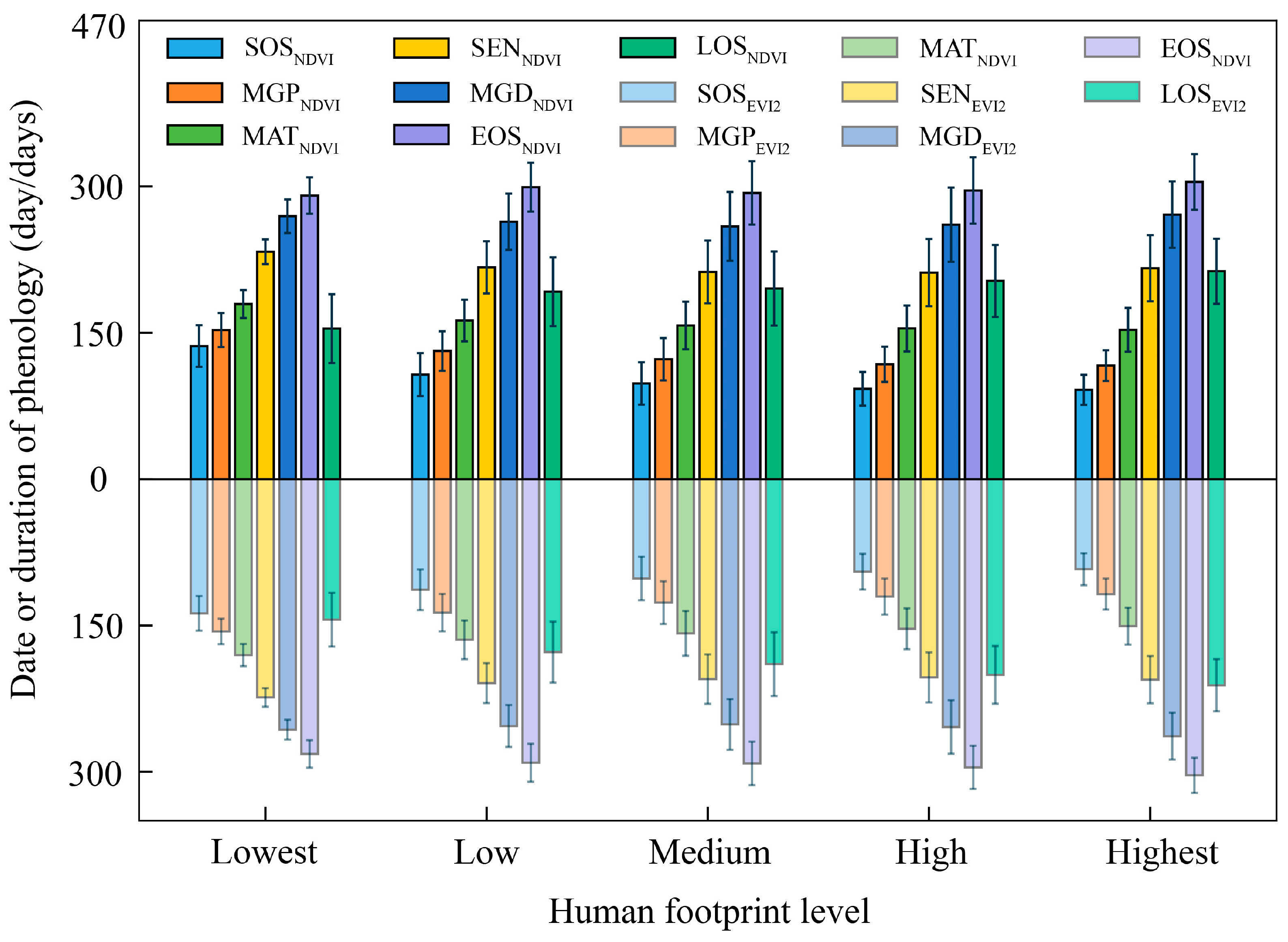
Figure 8 shows that as the human footprint gradient gradually increases, the SOS and EOS of NDVISDC and EVI2SDC show early greening and late dormancy. In the lowest and highest levels of human footprint, the SOS and EOS represented by NDVISDC (EVI2SDC) differed by 44.83 d (45.24 d) and 14.00 d (21.89 d). As the gradient of the human footprint increases, the LOS becomes longer.
Within the lowest and highest levels of human footprint, the differences in LOS for NDVISDC and EVI2SDC are 58.84 d and 67.13 d, respectively. MidGreenup, Maturity, and Senescence occur earlier with the increasing gradient of human footprint. Within the lowest and highest levels of human footprint, the differences in these phenological parameters for NDVISDC (EVI2SDC) are 36.44 d (38.28 d), 26.44 d (29.68 d), and 16.85 d (18.22 d), respectively.
Figure 9 shows the trends of LSP under different gradients of human footprint. Within the lowest level of human footprint, both NDVISDC and EVI2SDC show an overall trend of advancing from the SOS to the Senescence, while the MidGreendown to the EOS exhibits a delayed trend. The LOS for NDVISDC and EVI2SDC increases by 0.28 d yr−1 and 0.25 d yr−1, respectively. However, in the remaining scenarios, the MidGreendown and EOS show an overall trend of advancement. At the same time, the LOS exhibits a shortening trend. The largest reduction of LOS for NDVISDC and EVI2SDC is observed when the human footprint is in the range of 20–30, with an annual reduction of 0.86 d and 0.35 d, respectively.

4. Discussion

4.1. The Impact of Climate Change on LSP

Temperature, precipitation, and solar radiation were selected as climatic variables, and the response of each phenological parameter to climate variables was quantified by using the maximum partial correlation (Figure 10 and Figure S10). We found that the temperature was dominated by the negative correlation from the SOS to the Senescence, indicating that with the increase in temperature, the phenological period of vegetation greening was advanced. For EOS, the positive correlation was dominant, indicating that higher temperatures can prevent the decrease of vegetation chlorophyll caused by low temperatures and the discoloration of leaves caused by unsaturated membrane fatty acids [70], which delayed the autumn phenology, especially in high latitudes.
We found that temperature exhibits different responses to the SOS, MidGreenup, and Maturity in the HLAR. In high-latitude regions, elevated temperatures meet the heat requirements for early regreening of cold-adapted vegetation, promoting early regreening and growth [71]. However, in high-altitude areas such as the Qinghai-Tibet Plateau, there is a significant positive correlation between temperature and the greening phase of phenology, which can be attributed to the consumption of a significant amount of heat during the process of thawing frozen soil and increasing soil moisture, resulting in a gradual decrease in temperature and the early regreening of vegetation. Some studies suggest that vegetation on the Qinghai-Tibet Plateau is primarily controlled by precipitation. As temperatures increase, increased surface water evaporation delays vegetation regreening [72,73].
The proportional difference between the positive and negative correlations of radiation and precipitation throughout the entire phenological period is within 20%, which suggests that their influences on vegetation phenology in HLAR of the Northern Hemisphere are relatively balanced compared to temperature. Various vegetation types, geographical regions, and complex ecosystems cause different responses to precipitation and temperature, resulting in little difference in positive and negative partial correlations between radiation and precipitation on phenology. For example, in cold and wet regions, increased precipitation during spring is often accompanied by low temperatures, which negatively affect vegetation growth [66,74]. Conversely, in arid regions, higher temperatures promote vegetation growth. During the vegetation browning phase, increased precipitation is often accompanied by low temperatures and cloudiness, which reduce solar radiation and photoperiod in autumn and accelerate the accumulation of senescence enzymes and leaf aging. Additionally, the higher soil moisture resulting from increased precipitation is unfavorable for the growth of vegetation roots, leading to an early onset of dormancy [75]. In arid regions, increased solar radiation accelerates vegetation activity, shortens the growth cycle, promotes leaf senescence, and causes vegetation to enter dormancy earlier [76].
The predominant climatic factors driving the seven phenological characteristics in HLAR were studied by calculating the absolute maximum partial correlation coefficients between temperature, precipitation, and radiation (Table S4). Temperature accounts for more than 74% of the control over vegetation phenology in HLAR of the Northern Hemisphere for the SOS, MidGreenup, and Maturity. However, for the Senescence, MidGreendown, and EOS, the influence of temperature on vegetation phenology decreases significantly compared to the greening period. In contrast, the control effects of precipitation and radiation show an increasing trend, accounting for approximately 20–30% of the region, respectively. Nevertheless, temperature remains the primary factor governing vegetation senescence in HLAR in the Northern Hemisphere. In addition, the preseason length of the response of each phenological parameter to climate variables was studied (Figures S11–S16). The influence of temperature and solar radiation on the phenological parameters of the month is slightly greater than that of the preseason temperature and solar radiation from 1 to 4 months. Temperature with a preseason length of 1 month had a greater impact on SOS and MidGreenup. Temperature with a preseason length of 2 months has a greater impact on Maturity. The temperature of the month and the preseason length of 4 months have a greater impact on Senescence. The temperature of the month has a great influence on the MidGreendown and EOS.

4.2. The Effects of Global Greening on LSP

Researchers have developed a clear understanding of the trend change of LSP over time. However, there has been relatively limited exploration of the changes in NDVI or EVI2 during vegetation phenology, as well as the associated speed of vegetation development. Therefore, we calculated the monthly speed of vegetation development (VNDVI and VEVI2) based on NDVISDC and EVI2SDC, and discussed the changes in NDVI (EVI2) and the speed of vegetation development under vegetation phenology.
The VNDVI and VEVI2 of the SOS exhibit a positive development trend (Figure 11 and Figure S18), with the fastest vegetation development observed in June. However, there are significant variations in vegetation development among different phenological months. The speed of vegetation development is highest during the SOS in May and June, while it slows down during March and April. For the SOS derived from NDVISDC and EVI2SDC, the pixel proportion for March-April is 36.89% and 29.75%, respectively, whereas it increases to 62.34% and 69.32% for May–June (Figure S17), which indicates that vegetation with SOS occurring in May–June plays a dominant role in greening in HLAR.
During MidGreenup and Maturity, the speed of vegetation development slows down dominantly, while the trends in NDVISDC and EVI2SDC show an increasing pattern (Figures S19–S22). During the Senescence, the speed of vegetation senescence from September to November accelerates dominantly, and the trends of NDVISDC and EVI2SDC were increasing, and the pixel proportions reached 90.96% and 90.10%, respectively. For the EOS, NDVISDC and EVI2SDC accounted for 93.83% and 97.69% of the phenological pixels from September to November, of which the largest proportion was in October, reaching 44.87% and 60.58%. The speed of vegetation senescence from September to November is slowing down, and the trend is increasing significantly. Therefore, during the EOS, the vegetation dominated by October contributed the most to the greening of the HLAR. This study can be a useful supplement to Liu‘s view that June and October dominate greening in the Northern Hemisphere [77].
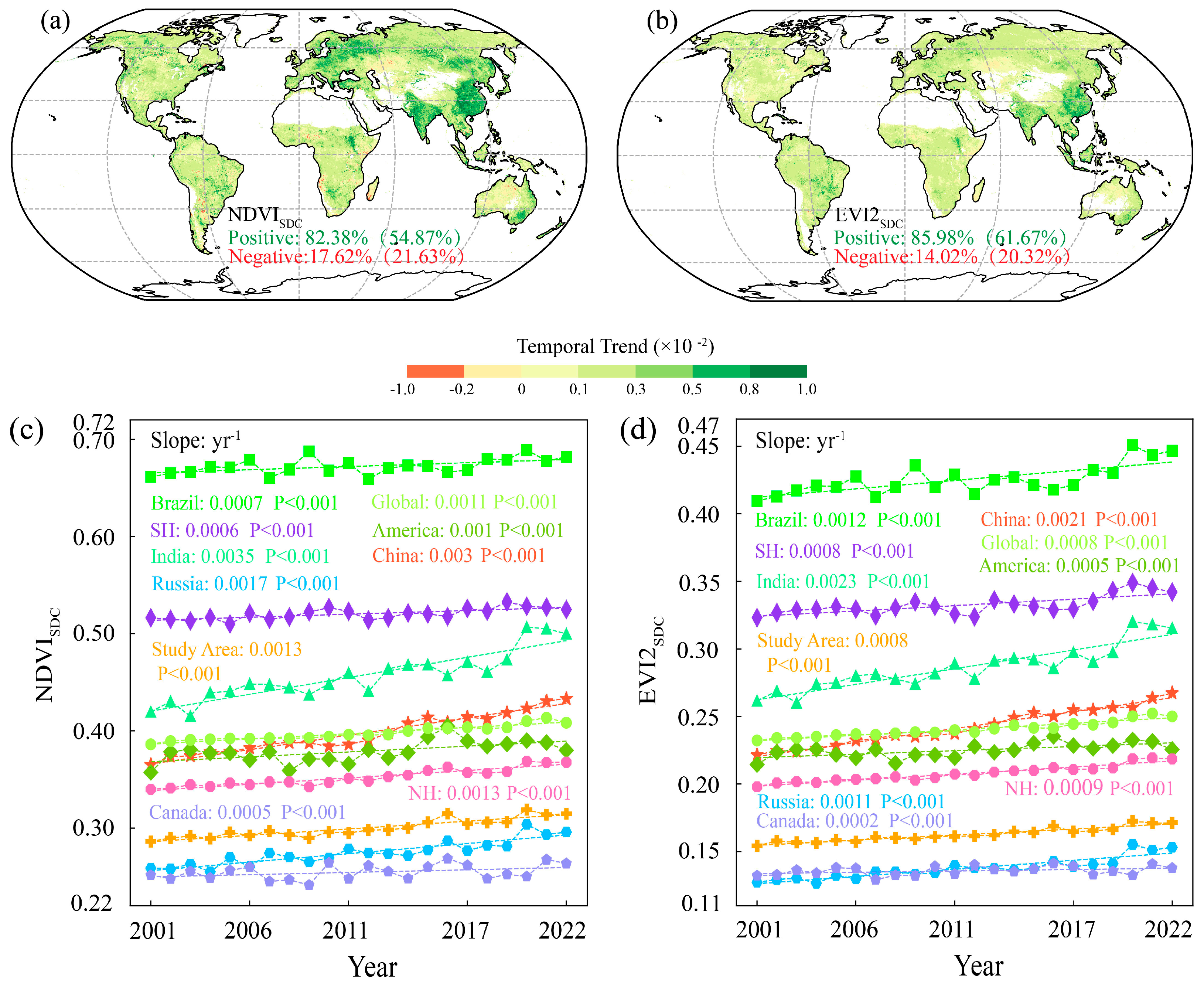
Based on the NDVISDC and EVI2SDC datasets, we conducted a trend analysis of NDVISDC and EVI2SDC from 2001 to 2022 at the global scale and in several typical regions. The results indicate that NDVISDC and EVI2SDC have 82.38% and 85.98% of the pixels showing a positive growth trend, and the proportion of significant pixels is 54.87% and 61.67%, respectively (Figure 12). Global NDVISDC (EVI2SDC) increased at a rate of 0.011 (0.008) decade−1. The greening rate in the Northern Hemisphere is higher than that in the Southern Hemisphere (NDVISDC: 0.013 vs. 0.006 decade−1; EVI2SDC: 0.009 vs. 0.008 decade−1). Among the continents (Figure S23), Europe exhibits the highest greening rate (NDVISDC(EVISDC): 0.022 (0.013) decade−1), followed by Asia (NDVISDC(EVISDC): 0.016 (0.011) decade−1), which are both higher than the overall global greening rate. The contributions of Asia and Europe to global greening, as revealed by NDVISDC and EVI2SDC, were 50.67% and 51.14%, respectively. Oceania had the smallest contribution to greening, with 4.10% for NDVISDC and 3.79% for EVI2SDC. At the national scale, China and India exhibit the most significant greening trends, with India having a higher greening rate than China (NDVISDC: 0.035 vs. 0.03 decade−1; EVI2SDC: 0.023 vs. 0.021 decade−1). Additionally, Russia shows a relatively fast greening trend among these countries (NDVISDC(EVI2SDC): 0.017 (0.011) decade−1), surpassing the global and Northern Hemisphere greening rates. Canada has the lowest greening rate among these countries (NDVISDC(EVI2SDC): 0.005 (0.002) decade−1). Russia’s relatively fast greening trend may be attributed to the increase in forest and grassland area by 79.27 km2×104 from 2001 to 2022. Additionally, with global climate warming, the extension of the vegetation growing period in high-latitude regions has increased the accumulation of NDVI and EVI. Human land use management is the main driving force behind land greening in China and India [78]. The rate of greening in India is dominated by cultivated land (69.30% for NDVISDC, 68.90% for EVI2SDC), and the rate of greening in China is dominated by grassland (66.31% for NDVISDC, 64.42% for EVI2SDC), as shown in Table S6. China‘s greening is mainly due to the gradual implementation of policies such as returning farmland to forests and grasslands for low-yielding fields in the past 20 years and the national construction of the Three-North Shelterbelt [79], which has led to a rapid increase in the area of green space and played an important role in improving land degradation, reducing surface temperature, and carbon storage [79,80,81]. India’s greening is primarily driven by the expansion of agricultural land and multiple cropping patterns. With India‘s growing population and food demand, India continues to increase the use of chemical fertilizers and irrigation of surface water and groundwater [82]. This pattern of greening may not be sustainable in the long term.

4.3. The Relationship between Different Vegetation Types and Vegetation Phenology

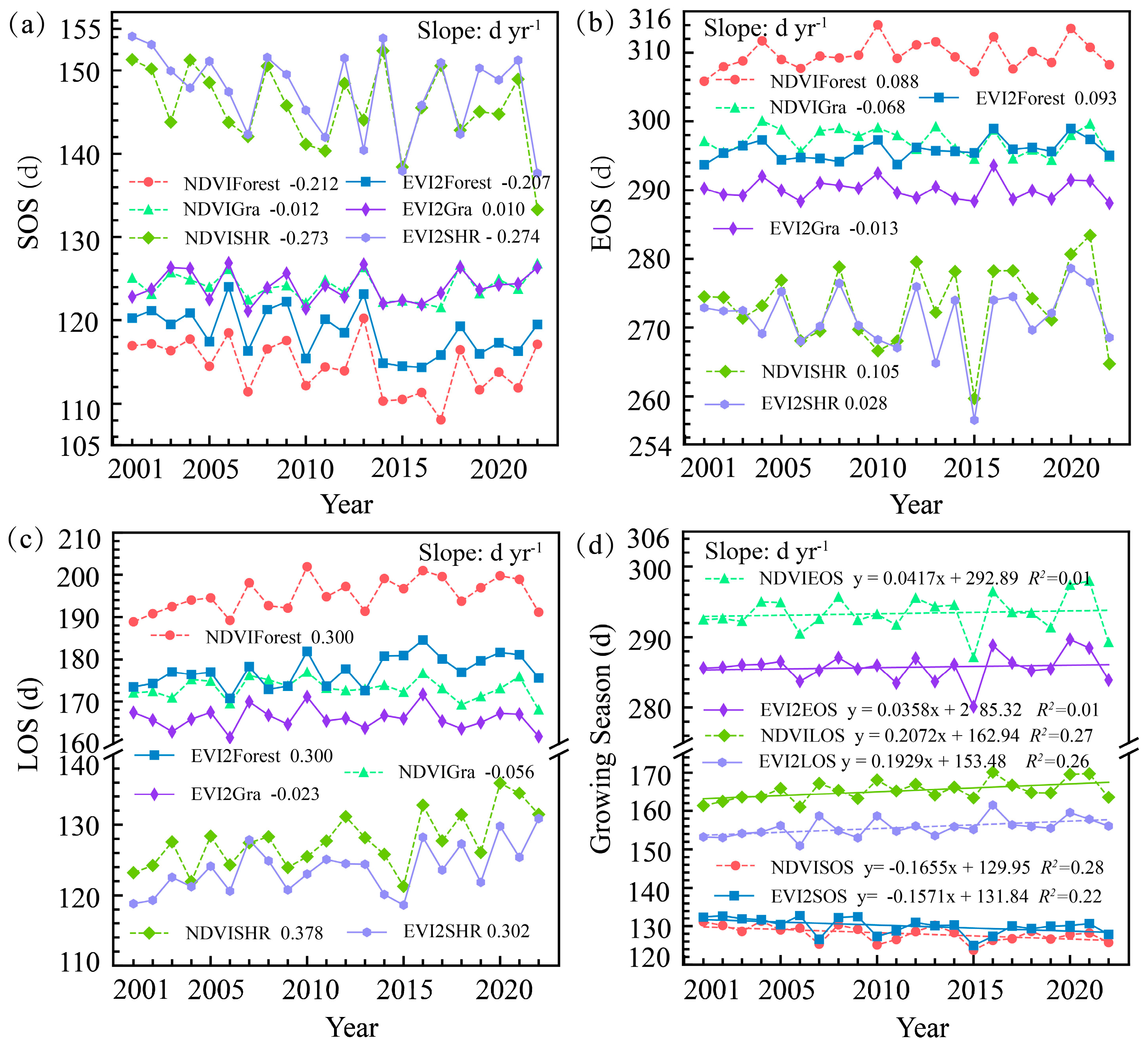
We analyzed the interannual variations of LSP for three vegetation types: forest, grassland, and shrub. NDVISDC and EVI2SDC exhibit the trends of these phenological parameters for each vegetation type, and the trend direction was basically similar. However, there are some discrepancies in the trend directions for grassland during the SOS and for shrubs during the MidGreenup. For instance, for the SOS of grassland, NDVISDC indicates an advancement of −0.012 d yr−1, while EVI2SDC shows a delay of 0.01 d yr−1. During the MidGreenup of shrubs, NDVISDC shows a delay of 0.069 d yr−1, whereas EVI2SDC shows an advancement of 0.102 d yr−1 (Figure 13 and Figure S24). The discrepancies in phenological trends shown by different datasets have also been reported in other studies [83]. The phenological stages of forests, including the SOS, MidGreenup, Maturity, Senescence, and MidGreendown, are all advancing at rates of −0.21 d yr−1, −0.16 d yr−1, −0.17 d yr−1, and −0.01 d yr−1 for NDVISDC, respectively. Similarly, for EVI2SDC, these stages are advancing at rates of −0.21 d yr−1, −0.14 d yr−1, −0.19 d yr−1, and −0.11 d yr−1. However, the EOS for forests is delaying by 0.09 d yr−1 for NDVISDC and 0.09 d yr−1 for EVI2SDC. The result also indicates that shrubs are experiencing changes in their phenological stages. Specifically, the SOS, MidGreenup, Maturity, and Senescence are all advancing at rates of −0.27 d yr−1, −0.24 d yr−1, −0.27 d yr−1, and −0.15 d yr−1 for NDVISDC, respectively. Similarly, for EVI2SDC, these stages are advancing at rates of −0.27 d yr−1, −0.26 d yr−1, −0.29 d yr−1, and −0.21 d yr−1. However, contrary to the trend in earlier stages, the EOS for shrubs is prolonging, with a rate of 0.11 d yr−1 for NDVISDC and 0.03 d yr−1 for EVI2SDC. From 2001 to 2022, in the overall phenological changes of forests, shrubs, and grasslands, the trend of SOS was advanced (NDVISDC: 1.7 d decades−1, EVI2SDC: 1.6 d decades−1), the trend of EOS was delayed (NDVISDC: 0.4 d decade−1, EVI2SDC: 0.4 d decade−1), and the trend of LOS is prolonged (NDVISDC: 2.0 d decades−1, EVI2SDC: 1.9 d decades−1).
Table 3 compares the phenological trends of different vegetation types. Due to the selection of different datasets, different phenological retrieval methods, different time spans, and different types of vegetation definitions, the same vegetation type may exhibit variations within the same region. Some scholars have compared vegetation phenology in the Northern Hemisphere (>30°) using the MOD13C1 and CIF datasets. They focused on secondary land cover types within different vegetation types, such as deciduous broadleaf forests, open shrublands, and sparse grasslands, to examine the phenological trends [83]. Researchers have conducted phenological studies in the temperate region of China, where the fastest advancement of SOS in the deciduous broadleaf forests was observed (13.6 d decade−1) [84]. In the Northern Hemisphere (>30°), the SOS of deciduous forests showed an advancement of 1.7 d decade−1 based on the MOD13C1 dataset and 1.3 d decade−1 based on the SIF dataset [83]. For mixed forests in the temperate region of China, the SOS advanced by 6.5 d decade−1 [84], while it advanced by 2.6 d decade−1 in mixed forests in the Northern Hemisphere (>40°) [85]. The SOS of deciduous coniferous forests exhibited an advancement of 3.3 d decade−1 from 1982 to 2014 in Xinjiang, China [86]. Some scholars have also studied the phenological trends of primary vegetation types in the Northern Hemisphere (>40°) from 1982 to 2013 and found that shrubs and grasslands have delayed SOS and EOS, and the LOS of shrubs is reduced by 0.1 d decade−1. In our study, shrubs showed earlier SOS and delayed EOS, with an extension of the LOS by 3.8 d decade−1 according to NDVISDC and 3.0 d decade−1 according to EVI2SDC. Additionally, forests and grasslands showed early SOS and delayed EOS from 1982 to 2014 in Northeast China, and the LOS of forests and grasslands was extended by 2.2 d decades−1 and 0.9 d decades−1 [87].

5. Conclusions

In this study, high temporal resolution MODIS products (NDVISDC and EVI2SDC) from 2001 to 2022 were used to explore the vegetation phenology in HLAR of the Northern Hemisphere from the perspective of human footprint and land use change, and the relationship between climate drive and vegetation greening and phenology was analyzed. The LSP characterized by EVI2SDC is later than NDVISDC in the development period of vegetation and earlier than NDVISDC in the senescence period of vegetation. From the analysis of time trends, the trend of the SOS, MidGreenup, Maturity, and Senescence is mainly in advance, and the MidGreendown to the EOS is mainly delayed. The LOS of NDVISDC and EVI2SDC was prolonged by 0.11 d yr−1 and 0.13 d yr−1, respectively. Among different vegetation types, the LOS of evergreen broadleaf forest was the longest (212.62 d), the LOS of open shrub was the shortest (118.92 d), and the deciduous coniferous forest exhibits the fastest rate of LOS extension (0.78 d yr−1). Regarding phenological changes under land use transitions of forests and grasslands, the LOS is the longest when the land is converted from built-up areas to forests and grasslands, with LOS values of 217.76 d (NDVISDC) and 209.0 d (EVI2SDC), respectively. In the expansion of cropland pattern, the conversion of forests to cropland has the highest LOS, with values of 197.62 d (NDVISDC) and 168.70 d (EVI2SDC), respectively.
Based on the analysis of temporal trends, in the case of most land cover conversion to cropland, the SOS is delayed and the EOS is advanced, which is contrary to the trend of most forests, grasslands, and shrubs. As the gradient of the human footprint gradually increases, the timing of SOS and EOS of NDVISDC and EVI2SDC appears earlier and later, but LOS shows a shortening trend. Temperature plays a predominant role in phenological responses, while the effects of precipitation and radiation on phenology are relatively balanced compared to temperature. At the same time, we supplemented the vegetation development and senescence months that play a key role in greening in the northern hemisphere. This study provides important insights into land use management under global climate change and enhances our understanding of global greening processes.

Supplementary Materials

The following supporting information can be downloaded at: https://www.mdpi.com/article/10.3390/rs16101744/s1, Figures S1–S24; Tables S1–S7.

Author Contributions

Conceptualization, X.M.; methodology, X.M.; validation, H.Y. (Hanmin Yin), Q.L. and Y.L.; resources, Q.L.; data curation, H.Y. (Hanmin Yin); writing—original draft preparation, H.Y. (Hanmin Yin) and Q.L.; writing—review and editing, H.Y. (Hanmin Yin) and Q.L.; supervision, X.L. and H.Y. (Huping Ye). All authors have read and agreed to the published version of the manuscript.

Funding

This research was funded by the Open Project of Key Laboratory, Xinjiang Uygur Autonomous Region (2023D04073), the Xinjiang Tianshan Youth Talent Top Project (2023TSYCCX0078), the Major Key Project of PCL, and the National Key Research and Development Program of China (2020YFA0608703).

Data Availability Statement

The MODIS Seamless Data Cube (SDC) is obtained from the Pengcheng Star Cloud platform (http://data.starcloud.pcl.ac.cn/resource/28, accessed on 1 May 2024).

Acknowledgments

We would like to thank NASA’s Land Process Distributed Active Archive Center (LPDAAC) (https://lpdaac.usgs.gov/, accessed on 1 May 2024) for the MOD11C3 and MCD12C1 datasets, the solar radiation and precipitation dataset provided by TerraClimate, the human footprint dataset shared by Haowei Mu, and the validation dataset provided by the United States National Phenology Network (USA-NPN) and the Pan-European Phenological Data Project (PEP27). Their contribution is crucial to the success of this project, and we sincerely thank them for their support.

Conflicts of Interest

The authors declare no conflicts of interest.

References

  1. Yang, Z.; Shen, M.; Jia, S.; Guo, L.; Yang, W.; Wang, C.; Chen, X.; Chen, J. Asymmetric responses of the end of growing season to daily maximum and minimum temperatures on the Tibetan Plateau. J. Geophys. Res. Atmos. 2017, 122, 13278–13287. [Google Scholar] [CrossRef]
  2. Piao, S.; Liu, Q.; Chen, A.; Janssens, I.A.; Fu, Y.; Dai, J.; Liu, L.; Lian, X.; Shen, M.; Zhu, X. Plant phenology and global climate change: Current progresses and challenges. Glob. Change Biol. 2019, 25, 1922–1940. [Google Scholar] [CrossRef] [PubMed]
  3. Li, P.; Liu, Z.; Zhou, X.; Xie, B.; Li, Z.; Luo, Y.; Zhu, Q.; Peng, C. Combined control of multiple extreme climate stressors on autumn vegetation phenology on the Tibetan Plateau under past and future climate change. Agric. For. Meteorol. 2021, 308, 108571. [Google Scholar] [CrossRef]
  4. Park, H.; Jeong, S.; Peñuelas, J. Accelerated rate of vegetation green-up related to warming at northern high latitudes. Glob. Change Biol. 2020, 26, 6190–6202. [Google Scholar] [CrossRef] [PubMed]
  5. Liu, Q.; Fu, Y.H.; Zeng, Z.; Huang, M.; Li, X.; Piao, S. Temperature, precipitation, and insolation effects on autumn vegetation phenology in temperate China. Glob. Change Biol. 2016, 22, 644–655. [Google Scholar] [CrossRef] [PubMed]
  6. Basler, D.; Körner, C. Photoperiod and temperature responses of bud swelling and bud burst in four temperate forest tree species. Tree Physiol. 2014, 34, 377–388. [Google Scholar] [CrossRef] [PubMed]
  7. Dong, L.; Wu, C.; Wang, X.; Zhao, N. Satellite observed delaying effects of increased winds on spring green-up dates. Remote Sens. Environ. 2023, 284, 113363. [Google Scholar] [CrossRef]
  8. Guo, M.; Wu, C.; Peng, J.; Lu, L.; Li, S. Identifying contributions of climatic and atmospheric changes to autumn phenology over mid-high latitudes of Northern Hemisphere. Glob. Planet. Change 2021, 197, 103396. [Google Scholar] [CrossRef]
  9. Chazdon, R.; Brancalion, P. Restoring forests as a means to many ends. Science 2019, 365, 24–25. [Google Scholar] [CrossRef]
  10. Keenan, T.F.; Gray, J.; Friedl, M.A.; Toomey, M.; Bohrer, G.; Hollinger, D.Y.; Munger, J.W.; O’Keefe, J.; Schmid, H.P.; Wing, I.S. Net carbon uptake has increased through warming-induced changes in temperate forest phenology. Nat. Clim. Change 2014, 4, 598–604. [Google Scholar] [CrossRef]
  11. Huntington, T.G. Climate change, growing season length, and transpiration: Plant response could alter hydrologic regime. Plant Biol. 2004, 6, 651–653. [Google Scholar] [CrossRef]
  12. Peñuelas, J.; Rutishauser, T.; Filella, I. Phenology feedbacks on climate change. Science 2009, 324, 887–888. [Google Scholar] [CrossRef] [PubMed]
  13. Griscom, B.W.; Adams, J.; Ellis, P.W.; Houghton, R.A.; Lomax, G.; Miteva, D.A.; Schlesinger, W.H.; Shoch, D.; Siikamäki, J.V.; Smith, P. Natural climate solutions. Proc. Natl. Acad. Sci. USA 2017, 114, 11645–11650. [Google Scholar] [CrossRef] [PubMed]
  14. Feng, X.; Fu, B.; Piao, S.; Wang, S.; Ciais, P.; Zeng, Z.; Lü, Y.; Zeng, Y.; Li, Y.; Jiang, X. Revegetation in China’s Loess Plateau is approaching sustainable water resource limits. Nat. Clim. Change 2016, 6, 1019–1022. [Google Scholar] [CrossRef]
  15. Delbart, N.; Kergoat, L.; Le Toan, T.; Lhermitte, J.; Picard, G. Determination of phenological dates in boreal regions using normalized difference water index. Remote Sens. Environ. 2005, 97, 26–38. [Google Scholar] [CrossRef]
  16. Helman, D. Land surface phenology: What do we really ‘see’ from space? Sci. Total Environ. 2018, 618, 665–673. [Google Scholar] [CrossRef] [PubMed]
  17. Lewis, S.L.; Wheeler, C.E.; Mitchard, E.T.; Koch, A. Restoring natural forests is the best way to remove atmospheric carbon. Nature 2019, 568, 25–28. [Google Scholar] [CrossRef]
  18. Buechel, M.; Slater, L.; Dadson, S. Hydrological impact of widespread afforestation in Great Britain using a large ensemble of modelled scenarios. Commun. Earth Environ. 2022, 3, 6. [Google Scholar] [CrossRef]
  19. Wang, L.; She, D.; Xia, J.; Meng, L.; Li, L. Revegetation affects the response of land surface phenology to climate in Loess Plateau, China. Sci. Total Environ. 2023, 860, 160383. [Google Scholar] [CrossRef]
  20. Hua, F.; Bruijnzeel, L.A.; Meli, P.; Martin, P.A.; Zhang, J.; Nakagawa, S.; Miao, X.; Wang, W.; McEvoy, C.; Peña-Arancibia, J.L. The biodiversity and ecosystem service contributions and trade-offs of forest restoration approaches. Science 2022, 376, 839–844. [Google Scholar] [CrossRef]
  21. Wang, C.; Zhang, W.; Li, X.; Wu, J. A global meta-analysis of the impacts of tree plantations on biodiversity. Glob. Ecol. Biogeogr. 2022, 31, 576–587. [Google Scholar] [CrossRef]
  22. Jia, Y.; Li, T.; Shao, M.a.; Hao, J.; Wang, Y.; Jia, X.; Zeng, C.; Fu, X.; Liu, B.; Gan, M. Disentangling the formation and evolvement mechanism of plants-induced dried soil layers on China’s Loess Plateau. Agric. For. Meteorol. 2019, 269, 57–70. [Google Scholar] [CrossRef]
  23. Zhou, G.; Xia, J.; Zhou, P.; Shi, T.; Li, L. Not vegetation itself but mis-revegetation reduces water resources. Sci. China Earth Sci. 2021, 64, 404–411. [Google Scholar] [CrossRef]
  24. Li, P.; Peng, C.; Wang, M.; Luo, Y.; Li, M.; Zhang, K.; Zhang, D.; Zhu, Q. Dynamics of vegetation autumn phenology and its response to multiple environmental factors from 1982 to 2012 on Qinghai-Tibetan Plateau in China. Sci. Total Environ. 2018, 637, 855–864. [Google Scholar] [CrossRef] [PubMed]
  25. Xin, Q.; Li, J.; Li, Z.; Li, Y.; Zhou, X. Evaluations and comparisons of rule-based and machine-learning-based methods to retrieve satellite-based vegetation phenology using MODIS and USA National Phenology Network data. Int. J. Appl. Earth Obs. Geoinf. 2020, 93, 102189. [Google Scholar] [CrossRef]
  26. Qi, Y.; Wang, H.; Ma, X.; Zhang, J.; Yang, R. Relationship between vegetation phenology and snow cover changes during 2001–2018 in the Qilian Mountains. Ecol. Indic. 2021, 133, 108351. [Google Scholar] [CrossRef]
  27. Ge, C.; Sun, S.; Yao, R.; Sun, P.; Li, M.; Bian, Y. Long-term vegetation phenology changes and response to multi-scale meteorological drought on the Loess Plateau, China. J. Hydrol. 2022, 614, 128605. [Google Scholar] [CrossRef]
  28. Zhu, Y.; Zhang, Y.; Zu, J.; Wang, Z.; Huang, K.; Cong, N.; Tang, Z. Effects of data temporal resolution on phenology extractions from the alpine grasslands of the Tibetan Plateau. Ecol. Indic. 2019, 104, 365–377. [Google Scholar] [CrossRef]
  29. Zhao, D.; Hou, Y.; Zhang, Z.; Wu, Y.; Zhang, X.; Wu, L.; Zhu, X.; Zhang, Y. Temporal resolution of vegetation indices and solar-induced chlorophyll fluorescence data affects the accuracy of vegetation phenology estimation: A study using in-situ measurements. Ecol. Indic. 2022, 136, 108673. [Google Scholar] [CrossRef]
  30. Zhao, Y.; Wang, M.; Zhao, T.; Luo, Y.; Li, Y.; Yan, K.; Lu, L.; Tran, N.N.; Wu, X.; Ma, X. Evaluating the potential of H8/AHI geostationary observations for monitoring vegetation phenology over different ecosystem types in northern China. Int. J. Appl. Earth Obs. Geoinf. 2022, 112, 102933. [Google Scholar] [CrossRef]
  31. Zhang, X.; Friedl, M.A.; Schaaf, C.B. Sensitivity of vegetation phenology detection to the temporal resolution of satellite data. Int. J. Remote Sens. 2009, 30, 2061–2074. [Google Scholar] [CrossRef]
  32. Kross, A.; Fernandes, R.; Seaquist, J.; Beaubien, E. The effect of the temporal resolution of NDVI data on season onset dates and trends across Canadian broadleaf forests. Remote Sens. Environ. 2011, 115, 1564–1575. [Google Scholar] [CrossRef]
  33. Cui, T.; Martz, L.; Zhao, L.; Guo, X. Investigating the impact of the temporal resolution of MODIS data on measured phenology in the prairie grasslands. GISci. Remote Sens. 2020, 57, 395–410. [Google Scholar] [CrossRef]
  34. Mu, H.; Li, X.; Wen, Y.; Huang, J.; Du, P.; Su, W.; Miao, S.; Geng, M. A global record of annual terrestrial Human Footprint dataset from 2000 to 2018. Sci. Data 2022, 9, 176. [Google Scholar] [CrossRef] [PubMed]
  35. Venter, O.; Sanderson, E.W.; Magrach, A.; Allan, J.R.; Beher, J.; Jones, K.R.; Possingham, H.P.; Laurance, W.F.; Wood, P.; Fekete, B.M. Sixteen years of change in the global terrestrial human footprint and implications for biodiversity conservation. Nat. Commun. 2016, 7, 12558. [Google Scholar] [CrossRef] [PubMed]
  36. Tucker, M.A.; Böhning-Gaese, K.; Fagan, W.F.; Fryxell, J.M.; Van Moorter, B.; Alberts, S.C.; Ali, A.H.; Allen, A.M.; Attias, N.; Avgar, T. Moving in the Anthropocene: Global reductions in terrestrial mammalian movements. Science 2018, 359, 466–469. [Google Scholar] [CrossRef] [PubMed]
  37. Hoffmann, S.; Irl, S.D.; Beierkuhnlein, C. Predicted climate shifts within terrestrial protected areas worldwide. Nat. Commun. 2019, 10, 4787. [Google Scholar] [CrossRef]
  38. Heck, E.; de Beurs, K.M.; Owsley, B.C.; Henebry, G.M. Evaluation of the MODIS collections 5 and 6 for change analysis of vegetation and land surface temperature dynamics in North and South America. ISPRS J. Photogramm. Remote Sens. 2019, 156, 121–134. [Google Scholar] [CrossRef]
  39. Wang, C.; Zhao, W.; Zhang, Y. The change in net ecosystem productivity and its driving mechanism in a mountain ecosystem of arid regions, Northwest China. Remote Sens. 2022, 14, 4046. [Google Scholar] [CrossRef]
  40. Zhao, Z.; Li, T.; Zhang, Y.; Lü, D.; Wang, C.; Lü, Y.; Wu, X. Spatiotemporal patterns and driving factors of ecological vulnerability on the Qinghai-Tibet Plateau based on the google earth engine. Remote Sens. 2022, 14, 5279. [Google Scholar] [CrossRef]
  41. Yang, S.; Zhao, Y.; Yang, D.; Lan, A. Analysis of Vegetation NDVI Changes and Driving Factors in the Karst Concentration Distribution Area of Asia. Forests 2024, 15, 398. [Google Scholar] [CrossRef]
  42. Piao, S.; Fang, J.; Zhou, L.; Ciais, P.; Zhu, B. Variations in satellite-derived phenology in China’s temperate vegetation. Glob. Change Biol. 2006, 12, 672–685. [Google Scholar] [CrossRef]
  43. Cong, N.; Wang, T.; Nan, H.; Ma, Y.; Wang, X.; Myneni, R.B.; Piao, S. Changes in satellite-derived spring vegetation green-up date and its linkage to climate in China from 1982 to 2010: A multimethod analysis. Glob. Change Biol. 2013, 19, 881–891. [Google Scholar] [CrossRef] [PubMed]
  44. Gao, M.; Wang, X.; Meng, F.; Liu, Q.; Li, X.; Zhang, Y.; Piao, S. Three-dimensional change in temperature sensitivity of northern vegetation phenology. Glob. Change Biol. 2020, 26, 5189–5201. [Google Scholar] [CrossRef]
  45. Liang, X.; Liu, Q.; Wang, J.; Chen, S.; Gong, P. Global 500 m seamless dataset (2000–2022) of land surface reflectance generated from MODIS products. Earth Syst. Sci. Data Discuss. 2023, 2023, 1–40. [Google Scholar] [CrossRef]
  46. Elmore, A.J.; Stylinski, C.D.; Pradhan, K. Synergistic Use of Citizen Science and Remote Sensing for Continental-Scale Measurements of Forest Tree Phenology. Remote Sens. 2016, 8, 502. [Google Scholar] [CrossRef]
  47. Templ, B.; Koch, E.; Bolmgren, K.; Ungersböck, M.; Paul, A.; Scheifinger, H.; Rutishauser, T.; Busto, M.; Chmielewski, F.-M.; Hájková, L. Pan European Phenological database (PEP725): A single point of access for European data. Int. J. Biometeorol. 2018, 62, 1109–1113. [Google Scholar] [CrossRef] [PubMed]
  48. Ma, Q.; Huang, J.-G.; Hänninen, H.; Berninger, F. Reduced geographical variability in spring phenology of temperate trees with recent warming. Agric. For. Meteorol. 2018, 256–257, 526–533. [Google Scholar] [CrossRef]
  49. Fu, Y.H.; Zhang, X.; Piao, S.; Hao, F.; Geng, X.; Vitasse, Y.; Zohner, C.; Peñuelas, J.; Janssens, I.A. Daylength helps temperate deciduous trees to leaf-out at the optimal time. Glob. Change Biol. 2019, 25, 2410–2418. [Google Scholar] [CrossRef]
  50. Paoli, A.; Weladji, R.B.; Holand, Ø.; Kumpula, J. The onset in spring and the end in autumn of the thermal and vegetative growing season affect calving time and reproductive success in reindeer. Curr. Zool. 2019, 66, 123–134. [Google Scholar] [CrossRef]
  51. Bórnez, K.; Descals, A.; Verger, A.; Peñuelas, J. Land surface phenology from VEGETATION and PROBA-V data. Assessment over deciduous forests. Int. J. Appl. Earth Obs. Geoinf. 2020, 84, 101974. [Google Scholar] [CrossRef]
  52. Liu, Y.; Wu, C.; Tian, F.; Wang, X.; Gamon, J.A.; Wong, C.Y.; Zhang, X.; Gonsamo, A.; Jassal, R.S. Modeling plant phenology by MODIS derived photochemical reflectance index (PRI). Agric. For. Meteorol. 2022, 324, 109095. [Google Scholar] [CrossRef]
  53. Xu, X.; Du, H.; Fan, W.; Hu, J.; Mao, F.; Dong, H. Long-term trend in vegetation gross primary production, phenology and their relationships inferred from the FLUXNET data. J. Environ. Manag. 2019, 246, 605–616. [Google Scholar] [CrossRef] [PubMed]
  54. Liu, Y.; Wu, C.; Wang, X.; Jassal, R.S.; Gonsamo, A. Impacts of global change on peak vegetation growth and its timing in terrestrial ecosystems of the continental US. Glob. Planet. Change 2021, 207, 103657. [Google Scholar] [CrossRef]
  55. Chang, Q.; Xiao, X.; Jiao, W.; Wu, X.; Doughty, R.; Wang, J.; Du, L.; Zou, Z.; Qin, Y. Assessing consistency of spring phenology of snow-covered forests as estimated by vegetation indices, gross primary production, and solar-induced chlorophyll fluorescence. Agric. For. Meteorol. 2019, 275, 305–316. [Google Scholar] [CrossRef]
  56. Fischer, A. A model for the seasonal variations of vegetation indices in coarse resolution data and its inversion to extract crop parameters. Remote Sens. Environ. 1994, 48, 220–230. [Google Scholar] [CrossRef]
  57. Rouse, J.W.; Haas, R.H.; Schell, J.A.; Deering, D.W. Monitoring vegetation systems in the Great Plains with ERTS. NASA Spec. Publ. 1974, 351, 309. [Google Scholar]
  58. Huete, A.; Didan, K.; Miura, T.; Rodriguez, E.P.; Gao, X.; Ferreira, L.G. Overview of the radiometric and biophysical performance of the MODIS vegetation indices. Remote Sens. Environ. 2002, 83, 195–213. [Google Scholar] [CrossRef]
  59. Hall, D.K.; Riggs, G.A. Normalized-difference snow index (NDSI). In Encyclopedia of Snow, Ice and Glaciers; Springer: Berlin/Heidelberg, Germany, 2010. [Google Scholar]
  60. Delloye, C.; Weiss, M.; Defourny, P. Retrieval of the canopy chlorophyll content from Sentinel-2 spectral bands to estimate nitrogen uptake in intensive winter wheat cropping systems. Remote Sens. Environ. 2018, 216, 245–261. [Google Scholar] [CrossRef]
  61. Chen, X.; Yang, Y. Observed earlier start of the growing season from middle to high latitudes across the Northern Hemisphere snow-covered landmass for the period 2001–2014. Environ. Res. Lett. 2020, 15, 034042. [Google Scholar] [CrossRef]
  62. Xu, D.; Wang, C.; Chen, J.; Shen, M.; Shen, B.; Yan, R.; Li, Z.; Karnieli, A.; Chen, J.; Yan, Y. The superiority of the normalized difference phenology index (NDPI) for estimating grassland aboveground fresh biomass. Remote Sens. Environ. 2021, 264, 112578. [Google Scholar] [CrossRef]
  63. Sen, P.K. Estimates of the regression coefficient based on Kendall’s tau. J. Am. Stat. Assoc. 1968, 63, 1379–1389. [Google Scholar] [CrossRef]
  64. Tošić, I. Spatial and temporal variability of winter and summer precipitation over Serbia and Montenegro. Theor. Appl. Climatol. 2004, 77, 47–56. [Google Scholar] [CrossRef]
  65. Cai, B.; Yu, R. Advance and evaluation in the long time series vegetation trends research based on remote sensing. J. Remote Sens. 2009, 13, 1170–1186. [Google Scholar]
  66. Xu, L.; Myneni, R.B.; Chapin Iii, F.S.; Callaghan, T.V.; Pinzon, J.E.; Tucker, C.J.; Zhu, Z.; Bi, J.; Ciais, P.; Tømmervik, H.; et al. Temperature and vegetation seasonality diminishment over northern lands. Nat. Clim. Change 2013, 3, 581–586. [Google Scholar] [CrossRef]
  67. Piao, S.; Wang, J.; Li, X.; Xu, H.; Zhang, Y. Spatio-temporal changes in the speed of canopy development and senescence in temperate China. Glob. Change Biol. 2022, 28, 7366–7375. [Google Scholar] [CrossRef]
  68. JEONG, S.-J.; HO, C.-H.; GIM, H.-J.; BROWN, M.E. Phenology shifts at start vs. end of growing season in temperate vegetation over the Northern Hemisphere for the period 1982–2008. Glob. Change Biol. 2011, 17, 2385–2399. [Google Scholar] [CrossRef]
  69. Wu, C.; Wang, X.; Wang, H.; Ciais, P.; Peñuelas, J.; Myneni, R.B.; Desai, A.R.; Gough, C.M.; Gonsamo, A.; Black, A.T. Contrasting responses of autumn-leaf senescence to daytime and night-time warming. Nat. Clim. Change 2018, 8, 1092–1096. [Google Scholar] [CrossRef]
  70. Matos, F.S.; de Oliveria, L.R.; de Freitas, R.G.; Evaristo, A.B.; Missio, R.F.; Cano, M.A.n.O.; dos Santos Dias, L.A. Physiological characterization of leaf senescence of Jatropha curcas L. populations. Biomass Bioenergy 2012, 45, 57–64. [Google Scholar] [CrossRef]
  71. Fu, Y.H.; Piao, S.; Vitasse, Y.; Zhao, H.; De Boeck, H.J.; Liu, Q.; Yang, H.; Weber, U.; Hänninen, H.; Janssens, I.A. Increased heat requirement for leaf flushing in temperate woody species over 1980–2012: Effects of chilling, precipitation and insolation. Glob. Change Biol. 2015, 21, 2687–2697. [Google Scholar] [CrossRef]
  72. Piao, S.; Cui, M.; Chen, A.; Wang, X.; Ciais, P.; Liu, J.; Tang, Y. Altitude and temperature dependence of change in the spring vegetation green-up date from 1982 to 2006 in the Qinghai-Xizang Plateau. Agric. For. Meteorol. 2011, 151, 1599–1608. [Google Scholar] [CrossRef]
  73. Shen, M.; Zhang, G.; Cong, N.; Wang, S.; Kong, W.; Piao, S. Increasing altitudinal gradient of spring vegetation phenology during the last decade on the Qinghai–Tibetan Plateau. Agric. For. Meteorol. 2014, 189, 71–80. [Google Scholar] [CrossRef]
  74. Liu, H.; Tian, F.; Hu, H.; Hu, H.; Sivapalan, M. Soil moisture controls on patterns of grass green-up in Inner Mongolia: An index based approach. Hydrol. Earth Syst. Sci. 2013, 17, 805–815. [Google Scholar] [CrossRef]
  75. Du, H.; Wang, M.; Liu, Y.; Guo, M.; Peng, C.; Li, P. Responses of autumn vegetation phenology to climate change and urbanization at northern middle and high latitudes. Int. J. Appl. Earth Obs. Geoinf. 2022, 115, 103086. [Google Scholar] [CrossRef]
  76. Yang, Y.; Guan, H.; Shen, M.; Liang, W.; Jiang, L. Changes in autumn vegetation dormancy onset date and the climate controls across temperate ecosystems in China from 1982 to 2010. Glob. Change Biol. 2015, 21, 652–665. [Google Scholar] [CrossRef] [PubMed]
  77. Liu, X.; Chen, Y.; Li, Z.; Li, Y. Greening in the middle and high latitudes in the Northern Hemisphere is determined by changes in the growth rate of natural vegetation during the growing season. Ecol. Indic. 2023, 155, 111025. [Google Scholar] [CrossRef]
  78. Chen, C.; Park, T.; Wang, X.; Piao, S.; Xu, B.; Chaturvedi, R.K.; Fuchs, R.; Brovkin, V.; Ciais, P.; Fensholt, R. China and India lead in greening of the world through land-use management. Nat. Sustain. 2019, 2, 122–129. [Google Scholar] [CrossRef] [PubMed]
  79. Zhang, Y.; Peng, C.; Li, W.; Tian, L.; Zhu, Q.; Chen, H.; Fang, X.; Zhang, G.; Liu, G.; Mu, X. Multiple afforestation programs accelerate the greenness in the ‘Three North’region of China from 1982 to 2013. Ecol. Indic. 2016, 61, 404–412. [Google Scholar] [CrossRef]
  80. Lu, F.; Hu, H.; Sun, W.; Zhu, J.; Liu, G.; Zhou, W.; Zhang, Q.; Shi, P.; Liu, X.; Wu, X. Effects of national ecological restoration projects on carbon sequestration in China from 2001 to 2010. Proc. Natl. Acad. Sci. USA 2018, 115, 4039–4044. [Google Scholar] [CrossRef]
  81. Tong, X.; Brandt, M.; Yue, Y.; Horion, S.; Wang, K.; Keersmaecker, W.D.; Tian, F.; Schurgers, G.; Xiao, X.; Luo, Y. Increased vegetation growth and carbon stock in China karst via ecological engineering. Nat. Sustain. 2018, 1, 44–50. [Google Scholar] [CrossRef]
  82. Lu, C.; Tian, H. Global nitrogen and phosphorus fertilizer use for agriculture production in the past half century: Shifted hot spots and nutrient imbalance. Earth Syst. Sci. Data 2017, 9, 181–192. [Google Scholar] [CrossRef]
  83. Chen, A.; Meng, F.; Mao, J.; Ricciuto, D.; Knapp, A.K. Photosynthesis phenology, as defined by solar-induced chlorophyll fluorescence, is overestimated by vegetation indices in the extratropical Northern Hemisphere. Agric. For. Meteorol. 2022, 323, 109027. [Google Scholar] [CrossRef]
  84. Zhou, X.; Geng, X.; Yin, G.; Hänninen, H.; Hao, F.; Zhang, X.; Fu, Y.H. Legacy effect of spring phenology on vegetation growth in temperate China. Agric. For. Meteorol. 2020, 281, 107845. [Google Scholar] [CrossRef]
  85. Zhao, J.; Zhang, H.; Zhang, Z.; Guo, X.; Li, X.; Chen, C. Spatial and temporal changes in vegetation phenology at middle and high latitudes of the Northern Hemisphere over the past three decades. Remote Sens. 2015, 7, 10973–10995. [Google Scholar] [CrossRef]
  86. Li, C.; Wang, R.; Cui, X.; Wu, F.; Yan, Y.; Peng, Q.; Qian, Z.; Xu, Y. Responses of vegetation spring phenology to climatic factors in Xinjiang, China. Ecol. Indic. 2021, 124, 107286. [Google Scholar] [CrossRef]
  87. Guo, J.; Hu, Y. Spatiotemporal variations in satellite-derived vegetation phenological parameters in Northeast China. Remote Sens. 2022, 14, 705. [Google Scholar] [CrossRef]
  88. Ma, R.; Shen, X.; Zhang, J.; Xia, C.; Liu, Y.; Wu, L.; Wang, Y.; Jiang, M.; Lu, X. Variation of vegetation autumn phenology and its climatic drivers in temperate grasslands of China. Int. J. Appl. Earth Obs. Geoinf. 2022, 114, 103064. [Google Scholar] [CrossRef]
Figure 1. Spatial distribution of land cover (a) and phenological observation sites (b) in the study area. The histogram in the bottom left corner (a) represents the regional proportions of different land cover types. The vegetation types at the phenological observation sites are primarily evergreen and deciduous forest.
Remotesensing 16 01744 g001
Figure 2. Comparison of phenological accuracy between LSP and phenological observations derived from the PEP27 dataset for deciduous broadleaf forests. The LSP of the year shows temporal consistency with the observed phenological stations in time. DBF is an abbreviation for deciduous broadleaf forest.
Remotesensing 16 01744 g002
Figure 3. The average spatial distribution and interannual variation of the human footprint in the study area. The left panel illustrates the average spatial distribution of the human footprint from 2001 to 2020. The right panel represents the interannual variation of the human footprint. The histogram in the left panel represents the proportion of different human footprints.
Remotesensing 16 01744 g003
Figure 4. The spatial distribution of multi-year average phenological parameters retrieved by NDVISDC and EVI2SDC in HLAR from 2001 to 2022. Histograms depict the frequency distribution of corresponding phenological dates. The LOS can be found in Figure S4.
Remotesensing 16 01744 g004
Figure 5. The spatial distribution of the temporal trends in HLAR from 2001 to 2022. Each histogram represents the frequency distribution of the corresponding trend. The black dots represent the trend pixels that have undergone a significant MK test (p < 0.05).
Remotesensing 16 01744 g005
Figure 6. The phenological differences of LSP based on the NDVISDC for LULCC in forests (a,e), shrubs (b,f), grasslands (c,g), and croplands (d,h). In panels (ad) and (eh), the first three or four boxplots represent the phenology under native vegetation. These boxplots are labeled using abbreviated phenological parameters. The naming rule of the remaining abscissa names is that the land cover type represented by the first letter (S: shrub, G: grassland, C: cropland, B: build-up, O: other land, W: water) is transferred to the land cover type represented by the second letter. The third letter or the third and fourth letters represent phenological parameters (S: SOS, E: EOS, L: LOS, MG: MidGreenup, MA: Maturity, SE: Senescence, MD: MidGreendown). The gray dotted line from top to bottom represents the average EOS, LOS, and SOS (ad) under different LULCC patterns, as well as the average MidGreendown, Senescence, Maturity, and MidGreenup (eh). The phenological differences of LSP retrieved by EVI2SDC are shown in Figures S7 and S8.
Remotesensing 16 01744 g006
Figure 7. Land use change patterns in forest, shrub, grassland, and cropland based on the phenological trend retrieved from NDVISDC. Each column in the picture represents the change in land use type. From left to right, the land cover type represented by the first letter (S: shrub, G: grassland, C: cropland, B: build-up, O: other land, W: water) is transferred to the land cover type represented by the second letter. Each row represents the corresponding phenological parameters. MGP, MAT, SEN, and MGD are abbreviations of MidGreenup, Maturity, Senescence, and MidGreendown. The black borders with trends greater than 0.35 or less than 0.35 are specially marked. Similarly, the trend distribution of EVI2SDC is shown in Figure S9.
Remotesensing 16 01744 g007
Figure 8. Vegetation phenology at different human footprint levels.
Remotesensing 16 01744 g008
Figure 9. The trend of LSP under different human footprint levels. Symbols *, **, and *** represent the significance levels at 95 % (p < 0.05), 99 % (p < 0.01), and 99.9 % (p < 0.001), respectively. The NDVI and EVI2 for each phenological parameter refer to the NDVISDC and EVI2SDC datasets, respectively.
Remotesensing 16 01744 g009
Figure 10. Spatial distribution of the partial correlation coefficients between phenological patterns (SOS and EOS) and climate variables (temperature, precipitation, and solar radiation) over the HLAR. The histograms represent the frequency distribution of the corresponding partial correlation coefficients.
Remotesensing 16 01744 g010
Figure 11. Monthly trends in VNDVI/EVI2 for SOS and EOS. Symbols ** and *** represent the significance levels at 99% (p < 0.01) and 99.9% (p < 0.001), respectively.
Remotesensing 16 01744 g011
Figure 12. Spatial trends and interannual variations of NDVISDC and EVI2SDC. (a,b) represent the spatial trends of global NDVISDC and EVI2SDC from 2001 to 2022, (c,d) represent the interannual trends in typical areas; SH represents the Southern Hemisphere; NH represents the Northern Hemisphere; and the Study area represents the HLAR. Green and red fonts represent the proportion of positive pixels and negative pixels, and the proportion of significant pixels is in parentheses for panels (a,b).
Remotesensing 16 01744 g012
Figure 13. The interannual phenological variations of forests, shrubs, and grasslands from 2001 to 2022. Panels (ac) represent the interannual variations of the SOS, EOS, and LOS for forests, shrubs, and grasslands, respectively. Panel (d) illustrates the overall phenological changes of forests, shrubs, and grasslands. The abbreviations “Gra” and “SHR” represent grasslands and shrubs, respectively.
Remotesensing 16 01744 g013
Table 2. The land use transfer matrix of the study area from 2001 to 2022 (× 104 km2).
2001GrasslandForestShrubCroplandBuilt-UpOther LandsWaterTotal
2022
Grassland2122.2116.985.645.40.950.367.02488.3
Forest97.7668.10.56.40.10.045.5778.34
Shrub41.81.0420.20.3--1.217.9482.4
Cropland41.13.00.2484.00.50.30.5529.6
Built-up0.70.2--0.820.70.010.0222.43
Other lands16.00.10.2-----565.01.2582.5
Water3.20.90.20.20.013.04360.04367.51
Total2322.7790.2506.9537.122.21619.854452.129251.08
Table 3. Comparison of LSP of forest, shrub, and grassland in different study regions.
Study AreaVegetation TypesPeriodsTrend (d yr−1)Satellite DataResolutionReference
SOSEOSLOS
The NH (>30°)DBF2001–2018−0.17−0.050.12MOD13C10.05°[83]
The NH (>30°)OS2001–2018−0.100.140.23MOD13C10.05°[83]
The NH (>30°)SA2001–2018−0.13−0.010.12MOD13C10.05°[83]
The NH (>30°)DBF2001–2018−0.13−0.080.06SIF0.05°[83]
The NH (>30°)OS2001–2018−0.06−0.010.05SIF0.05°[83]
The NH (>30°)SA2001–2018−0.13−0.020.11SIF0.05°[83]
The NH (>40°)MF1982–2013−0.260.350.61AVHRR GIMMS8KM[85]
The NH (>40°)Shrub1982–20130.080.07−0.01AVHRR GIMMS8KM[85]
The NH (>40°)GRA1982–20130.020.040.02AVHRR GIMMS8KM[85]
Temperate region China GRA1982–2015---0.16---AVHRR GIMMS8KM[88]
Temperate region ChinaMEA1982–2015---0.17----AVHRR GIMMS8KM[88]
Temperate region ChinaCNF1982–2015−1.08------AVHRR GIMMS8KM[84]
Temperate region ChinaMF1982–2015−0.65------AVHRR GIMMS8KM[84]
Temperate region ChinaDBF1982–2015−1.36------AVHRR GIMMS8KM[84]
Temperate region ChinaGRA1982–2015−0.33-------AVHRR GIMMS8KM[84]
Xinjiang, ChinaDNF1982–2014−0.30------AVHRR GIMMS8KM[86]
The Northeast ChinaForest1982–2014−0.060.160.22AVHRR GIMMS8km[87]
The Northeast ChinaGRA1982–2014−0.070.020.09AVHRR GIMMS8km[87]
The HLAR of NHForest2001–2022−0.210.090.30NDVISDC0.05°This study
The HLAR of NHGRA2001–2022−0.01−0.07−0.06NDVISDC0.05°This study
The HLAR of NHShrub2001–2022−0.270.110.38NDVISDC0.05°This study
The HLAR of NHForest2001–2022−0.210.090.30EVI2SDC0.05°This study
The HLAR of NHGRA2001–20220.01−0.01−0.02EVI2SDC0.05°This study
The HLAR of NHShrub2001–2022−0.270.030.30EVI2SDC0.05°This study
Note: DNF: Deciduous Needleleaf Forests, OS: Open Shrublands, SA: Savannas, CNF: Cold-temperate Needleleaf Forest, MF: Mixed Needle-leaf and Broadleaf Forests, DBF: Deciduous Broadleaf Forests, MEA:MEADOW.
Disclaimer/Publisher’s Note: The statements, opinions and data contained in all publications are solely those of the individual author(s) and contributor(s) and not of MDPI and/or the editor(s). MDPI and/or the editor(s) disclaim responsibility for any injury to people or property resulting from any ideas, methods, instructions or products referred to in the content.