Article

Constrained Iterative Adaptive Algorithm for the Detection and Localization of RFI Sources Based on the SMAP L-Band Microwave Radiometer

by
Xinxin Wang
1,2,3,
Xiang Wang
2,
Lin Wang
2,
Jianchao Fan
4 and
Enbo Wei
1,3,*
1
Key Laboratory of Ocean Observation and Forecasting and Key Laboratory of Ocean Circulation and Waves, Institute of Oceanology, Chinese Academy of Sciences, Qingdao 266071, China
2
National Marine Environmental Monitoring Center, Dalian 116023, China
3
University of Chinese Academy of Sciences, Beijing 100049, China
4
School of Control Science and Engineering, Dalian University of Technology, Dalian 116023, China
*
Author to whom correspondence should be addressed.
Remote Sens. 2024, 16(10), 1791; https://doi.org/10.3390/rs16101791
Submission received: 9 April 2024 / Revised: 12 May 2024 / Accepted: 16 May 2024 / Published: 18 May 2024

Abstract

:
The Soil Moisture Active Passive (SMAP) satellite carries an L-band microwave radiometer. This sensor can be used to observe global soil moisture (SM) and sea surface salinity (SSS) within the protected L-band spectrum (1400–1427 MHz). Owing to the complex effects of radio frequency interference (RFI), the SM and SSS data are missing or have low accuracy. In this paper, a constrained iterative adaptive algorithm for the detection, identification, and localization of RFI sources is designed, named MICA-BEID. The algorithm synthesizes antenna temperatures for the third and fourth Stokes parameters before RFI filtering, creating a new polarization parameter called WSPDA, designed to approximate the level of RFI interference on the L-band microwave radiometer. The algorithm then utilizes the WSPDA intensity and distribution density of RFI detection samples to enhance the identification and classification of RFI sources across various intensity levels. By utilizing statistical methods such as the probability density function (PDF) and the cumulative distribution function (CDF), the algorithm dynamically adjusts adaptive parameters, including the RFI detection threshold and the maximum effective radius of RFI sources. Through the application of multiple iterative clustering methods, the algorithm can adaptively detect and identify RFI sources at various satellite orbits and intensity levels. Through extensive comparative analysis with other localization results and known RFI sources, the MICA-BEID algorithm can achieve optimal localization accuracy of approximately 1.2 km. The localization of RFI sources provides important guidance for identifying and turning off illegal RFI sources. Moreover, the localization and long-time-series characteristic analysis of RFI sources that cannot be turned off is of significant value for simulating the spatial distribution characteristics of localized RFI source intensity in local areas.

1. Introduction

In recent years, observing soil moisture (SM) and sea surface salinity (SSS) with satellite-borne L-band microwave radiometers has become an emerging technology with broad scientific research and application prospects [1]. The Soil Moisture Active Passive (SMAP) satellite is the third scientific research satellite carrying an L-band microwave radiometer, following the Soil Moisture and Ocean Salinity (SMOS) and Aquarius/SAC-D satellites. It is mainly used to monitor global SM; however, it is also currently widely used in the satellite remote sensing observation of SSS due to its operating band and instrument design features [2,3,4,5].
The preferred band for the satellite observation of SM and SSS is 1413 MHz [6,7]. In accordance with the provisions in the Radio Regulations of International Telecommunications Union—Radiocommunication Sector (ITU-R), all emissions within the L-band frequency range from 1400 to 1427 MHz are prohibited [8,9]. However, numerous research results indicate that considerable radio frequency interference (RFI) has been observed worldwide for each satellite-borne L-band microwave radiometer [9,10,11,12,13,14]. Research institutes have taken into account RFI detection and mitigation methods in the design of each L-band microwave radiometer. Nevertheless, the unique design of the satellite sensor hardware alone cannot completely enable the detection and suppression of RFI, and different algorithms for radiation calibration, detection, and suppression are still required to alleviate the influences of RFI sources on L-band microwave radiometers [12,14,15].
Common L-band RFI sources primarily include radar systems, ground-based wireless services (such as monitoring cameras and WIFI networks), broadcasting satellite services, and meteorological satellite services [13,16]. These RFI sources are mainly distributed in large parts of Europe, Asia, and the Middle East [9,17]. Strong RFI emissions may cause abnormal increases in brightness temperature data, leading to significant data loss for scientific retrievals [9]. Moreover, weak RFI signals may be submerged in natural radiation signals, making them difficult to detect and identify and reducing the accuracy of SM and SSS inversion results, thus having a non-negligible influence on microwave radiometers [9,12,14].
The SMAP satellite carries an advanced L-band digital microwave radiometer that provides rich time and frequency sampling data, offering more support for RFI detection and suppression [11,18]. The integrated detection and suppression algorithms used by the SMAP satellite include time domain detection, cross-frequency detection, kurtosis detection, and polarimetric RFI detection algorithms. The output flag results from these RFI detectors are integrated through the maximum probability of detection (MPD) algorithm to reach the MPD and remove the RFI-corrupted pixels in each footprint [18,19,20]. In recent years, machine learning methods have been applied for RFI detection and localization using SMAP data. Soldo et al. (2018) proposed a method that employs Density-Based Spatial Clustering for Applications with Noise (DBSCAN) along with centroid calculation to estimate the location of RFI sources [14]. Nazar et al. (2023) conducted a multi-dimensional semi-supervised learning approach [21]. Owfi et al. (2023) proposed an autoencoder-based RFI mitigation method [22]. These methods offer novel detection strategies to address the complex and variable characteristics of RFI. Furthermore, they enhance our understanding of the characteristics of RFI.
China is within the influential range of terrestrial RFI, so satellite observation data of earth surface brightness temperature are of low quality, further influencing the accuracy of inverted SM and SSS data and seriously constraining the research and service applications of satellite-borne L-band microwave radiometers [23,24]. The diverse types and varying intensities of RFI sources, widely distributed on land, coupled with the spatiotemporal variability of overlapping RFI signals, make the impact on L-band microwave radiometers extremely complex and difficult to suppress effectively.
Given the sensitivity of the third and fourth Stokes parameters of L-band microwave radiometers to RFI, we have constructed a polarization parameter and evaluated its capability to characterize RFI features. Based on the intensity and spatiotemporal distribution characteristics of this polarization parameter, a constrained iterative adaptive algorithm for RFI sources detection, clustering, identification, and localization using machine learning methods is designed. The algorithm is applied to analyze and identify the localization of various types of RFI sources using SMAP satellite L-band microwave radiometer data. The results provide important technical support for both locating and turning off illegal RFI sources, enhancing the accuracy of retrieval data. As China’s ocean salinity satellite approaches launch, this study is essential for developing SSS retrieval algorithms capable of effectively detecting and mitigating interference effects from RFI.

2. Materials and Methods

2.1. SMAP L1B_TB Data

In this study, we utilized the SMAP Level 1B Brightness Temperature Product (L1B_TB) provided by the NASA National Snow and Ice Data Center (NSIDC). This Level-1B product provided calibrated estimates of time-ordered geolocated brightness temperatures measured by the SMAP passive microwave radiometer. The algorithm established in this study primarily utilized the antenna temperatures for the third and fourth Stokes parameters, denoted as ta_3 and ta_4, for each footprint before RFI filtering. The RFI original detection flag (tb_qual_flag_3/4/h/v) and the longitude and latitude of the intersection of the antenna boresight vector and the Earth’s surface (tb_lon and tb_lat) are used as inputs, as distributed in the L1B_TB products of SMAP.

2.2. Theoretical Analysis of RFI Influence Characteristics

The Stokes parameter matrix of polarization data from satellite-borne L-band microwave radiometers contains four Stokes parameters representing the polarization characteristics of ground object microwave radiation. The third and fourth Stokes parameters are proportional to the real and imaginary parts of the correlation between fields in horizontal and vertical polarizations, respectively. The modified Stokes vector expressed with brightness temperature is as follows [25,26]:
T B = T h T v T 3 T 4 = λ 2 k B η E h 2 E v 2 2 R e E v E h * 2 I m E v E h *
where λ is the radiometer’s wavelength, k is Boltzmann’s constant, B is the bandwidth, η is the medium impedance (air), and Ev and Eh are the two orthogonal components of the plane wave, which are electric field strengths in vertical and horizontal directions, respectively.
Under the natural-level conditions uncontaminated by RFI, the third and fourth Stokes parameters of L-band microwave radiometers are very small [27]. However, these parameters are highly sensitive to signals from ground-based RFI, and their anomalies can indicate the presence and characteristics of various RFI sources and can also reflect RFI signals at different intensity levels; in particular, they have some advantages in the detection of weak RFI signals. In addition, the synthesized parameters of the third and fourth Stokes parameters can characterize the emission intensity of terrestrial RFI sources to a certain extent [11,21,27,28,29].
The synthesis parameter detection algorithm (SPDA), established through the synthesis of dual parameters, can simultaneously identify artificial RFI sources with linear polarization and those with circular polarization. It effectively covers the present polarization modes of artificial radiation sources, achieving the purpose of comprehensive RFI detection. The expression for the synthesized polarization characteristic parameter is as follows [28]:
W S P D A = T 3 2 + T 4 2
Substituting T3 and T4 in Equation (1) into Equation (2) yields [21]:
W S P D A = 2 λ 2 k B η E 0 h t E 0 v t
where E 0 h and E 0 v represent the amplitudes of electric field strength under horizontal and vertical polarizations, respectively.
It can be seen that the synthesized polarization parameter WSPDA is directly proportional to the time-averaged product of horizontally and vertically polarized amplitudes of plane waves. The radiated power is directly proportional to the square of the amplitude of a plane wave. This relationship indicates that, under ideal conditions, the polarization parameter WSPDA can be used to estimate the impact strength of RFI sources on L-band microwave radiometers.
For an RFI source located in the effective field of view (EFOV) of the antenna of a radiometer, if the effective isotropic radiated power (EIRP) emitted from the RFI source points to the satellite, the interference signal can easily enter the receiving antenna of the microwave radiometer. The EIRP represents the power radiated from a directional antenna in its maximum radiation direction, and it is usually used to characterize the emissive capability of a ground-based transmitting system [21,30] based on the following formula:
E I R P = P t G t
where P t represents transmission power, and G t represents the gain of the transmitting antenna.
The Friis transmission equation can determine the relationship between received power, antenna gain, and transmission power [30]. According to the Friis transmission equation, the EIRP can be calculated using the following formula [31]:
E I R P = 4 π R λ 2 P r G r
where P r represents the received power, G r represents the gain of the receiving antenna, R represents the distance between the two antennas, and λ represents the wavelength.
The relationship between the WSPDA of the satellite receiving antenna and the EIRP of a ground-based RFI source can be established with the Friis transmission formula [31]:
P t G t θ r , φ r = k B 4 π R λ 2 W S P D A G r θ t , φ t
where P t G t θ r , φ r represents the EIRP of the RFI source in the direction of the L-band microwave radiometer experiencing interference, and G r θ t , φ t represents the gain of the receiving antenna in the direction of the RFI source.
As can be discerned from Equation (6), the parameters of the ground-based RFI source, including transmission power and the gain of the transmitting antenna, remain unknown. Additionally, the transmission power may fluctuate dynamically over time. Furthermore, the orientation of both the RFI source antenna and the satellite sensor antenna is also unknown. The WSPDA for continuous instantaneous observations can be used to characterize the spatiotemporal variation characteristics of the interference intensity from the land-based RFI source to the L-band microwave radiometer.
To minimize the RFI noise received by the satellite antenna, the main lobe direction of the satellite antenna should avoid the emission directions of the antenna of strong RFI noise sources in principle, and the sidelobes in the pattern of the satellite antenna should be reduced or lowered. However, since ground-based RFI sources are of widespread distribution, the emission directions of the antenna of RFI sources are varied, and the satellite antenna has different observation elevations and azimuths, it is challenging to entirely avoid RFI sources. Establishing the aforementioned multivariate functional relationships can help us quantitatively understand the spatial distribution characteristics of terrestrial RFI sources on satellite observation data and is crucial for the establishment of RFI identification and localization algorithms.

2.3. SMAP RFI Detection Algorithm

The SMAP satellite uses multiple RFI detection algorithms. The composite MPD RFI detection algorithm employs a logical OR operation on each of the individual RFI detection flags, and it is used to achieve the purpose of reaching the MPD [18,19,20,32]. Compared with the SMOS, the SMAP is less affected by RFI in the coastal ocean regions [33]. The RFI detection algorithms designed for the SMOS, Aquarius, and SMAP satellites according to the features of the onboard radiometers have a common characteristic: a fixed or dynamic threshold needs to be set by RFI characteristics to realize detection filtering and control false alarm rate (FAR). However, the threshold has two sides: if the threshold is set too low, the FAR will be increased; if the threshold is set too high, the probability of detection (PD) will be decreased. In addition, these ordinary and direct methods mainly suffer from the following potential limitations:
(1)
Weak RFI sources may be submerged into the action range of strong RFI sources or into natural-level radiation signals, making them difficult to detect [12,18].
(2)
The substantial transition in brightness temperature that occurs at land–water and ice–water boundaries can also cause false alarms. Several algorithms have too high FAR at land–water and ice–water coastal boundaries, and only increasing the threshold can be used to reduce the FAR. However, increasing the threshold may result in the missed detection of weak RFI at coastal boundaries [11,12].
(3)
The influence of an RFI source on a satellite-borne L-band microwave radiometer through sidelobes is not limited by the RFI source position. As long as there is a line-of-sight propagation path between the transmitting antenna and the receiving antenna, the RFI source will influence the satellite observation results [12,14,34,35].
(4)
The emission characteristic of terrestrial RFI sources dynamically varies over time, and this increases the difficulty in setting a threshold for the detection algorithm [12].
(5)
Polarization can precisely characterize the RFI signal, but the utilization rate of polarization detection algorithms is too low in actual applications because of the influences of Faraday rotation and coastal boundaries [11,19,28].

2.4. Construction of RFI Detection, Identification, and Localization Algorithms

To better utilize polarization data, we, making use of the characteristic that the SMAP third and fourth Stokes parameters are sensitive to RFI sources, constructed a synthesized polarization parameter, WSPDA. Based on the spatial distribution of WSPDA, we established a constrained iterative adaptive algorithm for RFI detection, identification, and localization. The algorithm was developed based on the Interactive Data Language (IDL) 8.5 platform and included an RFI sample detection module, an iterative clustering module, and an RFI identification and localization module. Figure 1 illustrates the steps of the constrained iterative adaptive algorithm.
In Figure 1, Y_i_j, where i represents the number of iterations and j represents the number of generated clustering clusters, Wmax is the maximum value of WSPDA within a clustering cluster, and Rmax is the maximum action radius at the location where Wmax is found. In each iteration, the samples for the newly generated database are sourced from those outside the boundary conditions established during the previous clustering. The samples that are not identified as RFI are flagged as ‘No RFI’ and are excluded from all subsequent iterations. The following outlines the specific steps of the algorithm:
  • Step I: Detect and extract suspected RFI samples
The third and fourth Stokes parameters are extracted from the SAMP L1B data, and the parameter WSPDA characterizing the satellite-received RFI radiation intensity is calculated with Equation (2). Subsequently, statistical methods, as detailed in Equation (7), are applied to calculate both the probability density function (PDF) and the cumulative distribution function (CDF) for the WSPDA data across half-orbit. Based on the conducted statistical analysis, in this study, the cumulative probability is established as an empirical constant of 95%. The calculated value of w then serves as the detection threshold, denoted by Wd. This 95% value represents the chosen level of significance for RFI detection specific to the scope and objectives of this research.
F W S P D A w = P W S P D A w
where P is the probability density value of parameter WSPDA and F W S P D A w is the cumulative distribution value of parameter WSPDA.
This threshold Wd was dynamic and obtained based on the statistical characteristics of each orbit. In summary, the RFI detection sample dataset is a union of the datasets generated under the following two conditions:
S M A P   R F I   d e t e c t i o n   f l a g S R D F = Y e s
W S P D A   W d
  • Step II: Perform iterative clustering of RFI samples
A multiple iterative clustering algorithm based on emission intensity and density (MICA-BEID), which simultaneously considers the emission intensity and distribution density of the RFI source, is used for the sample data. By adding a maximum radius of action of the RFI sources as a boundary condition, a bounded multiple iterative clustering algorithm is constructed. This algorithm is then used to obtain clusters.
  • Step III: Identify and localize RFI sources
Whether a cluster contains RFI sources is determined according to the spatial distribution of the RFI sample intensity in the cluster. When a cluster contains RFI sources, the coordinates of the maximum WSPDA in the cluster are extracted to obtain single-time RFI source location information. Subsequently, the centroid of a long-time-series multi-orbit RFI source location dataset is then calculated to establish the RFI source’s final location [14].

3. Results

3.1. Detection of RFI Suspected Samples

3.1.1. Extraction of RFI Detection Samples

Rational classification of RFI detection samples based on the intensity and spatial distribution characteristics of RFI detection results is crucial for detecting RFI sources across various energy levels. Spatially continuous and sufficient RFI detection samples are a precondition for classification. In fact, the SMAP satellite, equipped with an advanced L-band microwave radiometer, acquires rich time–frequency data. This capability allows it to employ multiple RFI detection algorithms. Consequently, the RFI flags in the SMAP L1B data can provide a large quantity of detection flag samples for RFI classification. However, owing to such factors as Faraday rotation and rapid variation in brightness temperature at coastal boundaries, the threshold for the polarization detection algorithm used by the SMAP satellite is set to a very high value, and the polarization characteristics of the RFI signal are not fully utilized in actual applications. Therefore, in this study, in addition to the original RFI flag samples extracted from the SMAP L1B data, the RFI detection samples were supplemented using the SPDA detection algorithm.
Figure 2 shows a statistical histogram of the SMAP half-orbit data WSPDA. It can be seen from the statistical results of the ascending and descending orbits that 95% of the samples are primarily distributed in a threshold interval of [0, 6.3 K] and [0, 5.5 K], respectively. The detection thresholds Wd for RFI polarization detection in the ascending and descending orbits were set to 6.3 K and 5.5 K, respectively.
Nevertheless, RFI detection samples on the edges of the satellite orbit may be affected by RFI sources outside the satellite orbit strip so there may be no RFI sources in the RFI detection samples on the orbit edges. These RFI detection samples can be removed based on the scan angle range of the SMAP satellite. To avoid such cases, clusters were discarded if the cluster’s center corresponded to a scan angle of 90° ± 25° (left side of the scan) or 270° ± 25° (right side of the scan) [14].
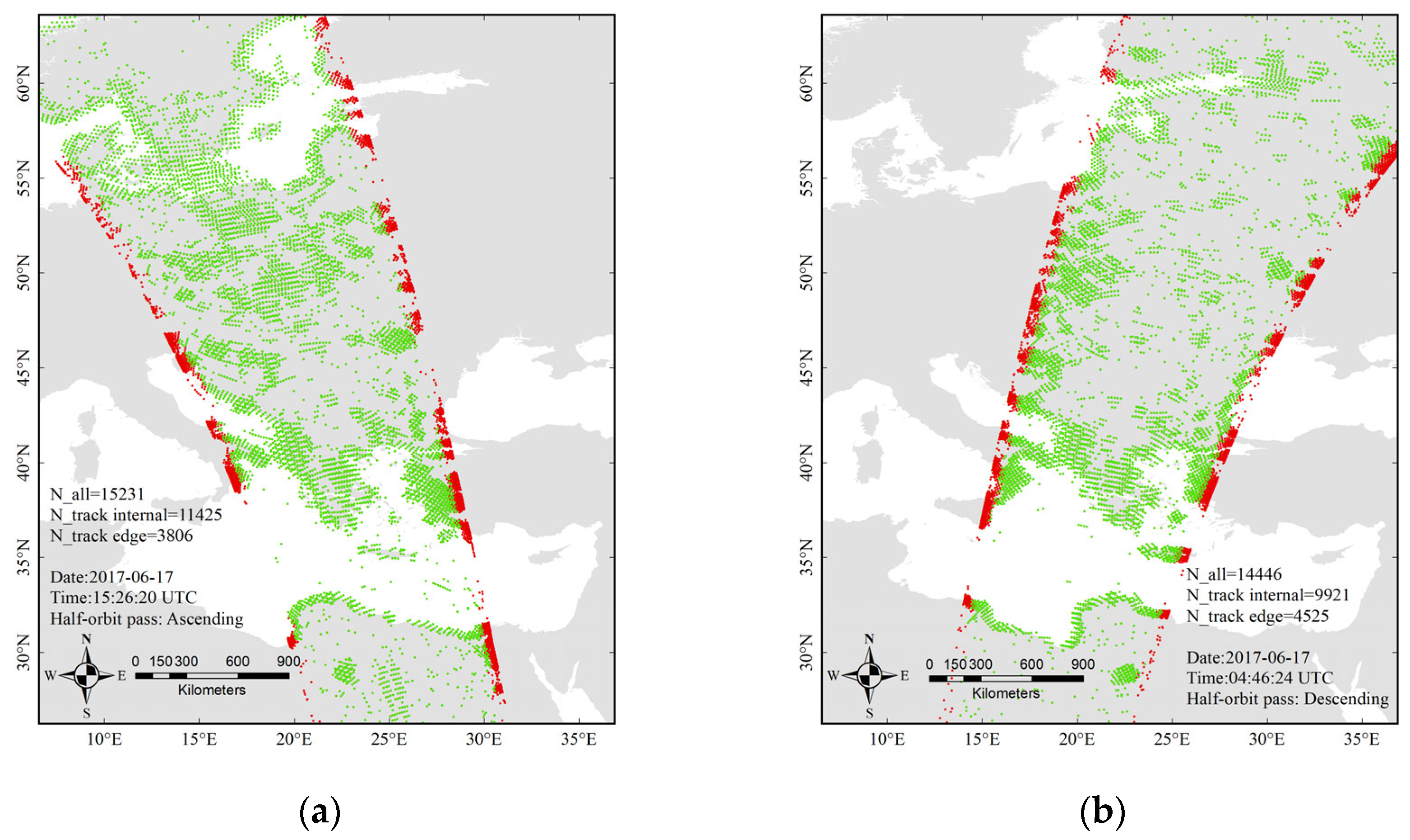
Figure 3a,b show schematic maps of the spatial distribution of RFI detection sample data on the SMAP satellite orbit edge (red) and inside orbit (green) for two orbits (ascending and descending orbits) obtained on 17 June 2017. Figure 3c,d show schematic maps of the spatial distribution of an RFI detection sample dataset of SMAP data with samples on orbit edges being removed for two orbits (ascending and descending orbits) obtained on 17 June 2017, where the SPDA detection samples are in red, the SRDF samples are in blue, and the overlapped samples are in green. Table 1 shows the results of the RFI detection based on SMAP L1B half-orbit data (from ascending and descending orbits). As can be seen from the figures and table, the number of SPDA detection samples is greater than that of the SRDF samples on both ascending and descending orbits. Both SPDA detection samples and SRDF samples exhibit basically consistent spatial distributions in the zones, with SRDF samples being more concentrated, and the sample overlap rate accounts for over 50% of the total SRDF samples. However, at coastal boundaries, the number of SPDA detection samples is far greater than that of SRDF samples.
We have discussed potential limitations with the SMAP RFI detection algorithms at coastal boundaries in Section 2.3. The thresholds for the SMAP RFI third Stokes detector remain high, essentially not contributing to the overall FAR. To avoid excessive false alarms at coastal crossings, the thresholds for the SMAP pulse and fourth Stokes detectors are increased on coastal boundaries [11]. For the reasons mentioned above, there is a risk of missing the detection of RFI sources at sea–land and sea–ice boundaries.
The SPDA detection method relies on the statistical characteristics of natural-level radiation signals, and it can effectively supplement weak RFI signal detection samples and address the issue of missing RFI samples at the water–land boundary. However, the threshold for SPDA is a dynamic value obtained based on statistics, and the probability of 95% is an empirical value, so the dynamic threshold method still cannot fully cover all RFI samples. If the selected threshold is too low, both PD and FAR will increase during RFI detection. This could lead to a large quantity of falsely detected RFI detection samples, thus reducing the running efficiency of detection and localization algorithms. Conversely, if the selected threshold is too high, there is a risk of missing RFI signals at a low energy level. Comprehensive consideration of the SRDF samples being selected for sample supplementation and the detection samples obtained with other algorithms being used as auxiliary inputs can well solve the problems of false and missed detection. The method of combining the SPDA detection algorithm and the SRDF not only covers RFI weakly contaminated signal samples but also supplements RFI detection samples at coastal boundaries, ensuring the comprehensive coverage of RFI detection samples.

3.1.2. Classification of RFI Detection Samples at the Water–Land Boundary

The RFI signals at the water–land boundary cannot be extracted effectively using the initially set dynamic threshold, as the background value of parameter WSPDA at the water–land boundary is higher than that in other areas. Therefore, it is necessary to establish a dynamic threshold for RFI detection samples at the water–land boundary through statistical analysis. This adjusted threshold helps to eliminate abnormal background gain values and obtain RFI detection samples at the water–land boundary:
W S P D A _ c o a s t l i n e s = W w a t e r l a n d _ c o n t a m i n a t i o n + W R F I
where W w a t e r l a n d _ contamination is the total contribution at the water–land boundary under natural-level conditions, and W R F I is the unwanted contributions caused by RFI.
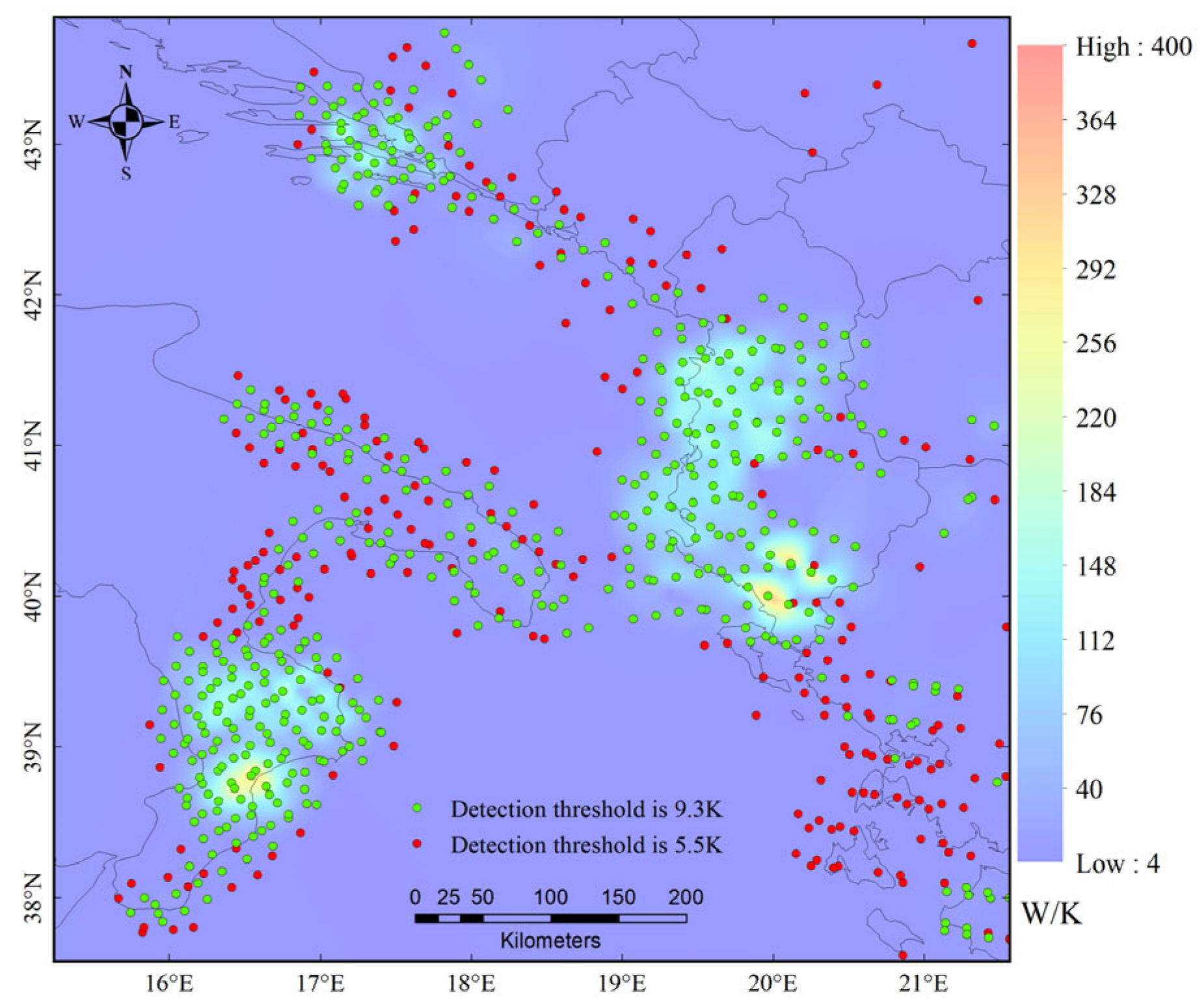
By calculating the PDF and CDF for the WSPDA data at the water–land boundary, the detection thresholds Wd for RFI detection samples in the ascending and descending orbits were set to 10.6 K and 9.3 K, respectively. These thresholds are dynamic and obtained based on the statistical characteristics of each orbit. As illustrated in Figure 4, adjusting the detection threshold at the water–land boundary effectively removes most abnormal contributions within the water–land boundary belt and can retain the RFI detection flag samples to the maximum extent.

3.2. Iterative Clustering of RFI Samples

The clustering classification of RFI samples was conducted using the DBSCAN method, and a region with sufficiently high density can be delimited as a cluster by calculating the maximum set of density-connected points to construct an RFI cluster [14,36]. Nevertheless, clusters in many shapes can also be found in a spatial sample dataset of noise using the DBSCAN method. In terrestrial areas, numerous RFI detection samples around multiple adjacent RFI sources may be clustered into a single cluster. Additionally, at the water–land boundary, banded clusters may be formed along the coastal belt. The formation of these clusters is primarily determined by the spatial distribution of the RFI detection samples. Therefore, it is required to establish a MICA-BEID algorithm by analyzing the spatial distribution characteristic of clusters, coupled with an iterative calculation, to realize the multi-level classification of the RFI detection samples from strong to weak and the identification and localization of RFI sources.

3.2.1. DBSCAN Clustering

Two critical parameters—the scan radius (R) and the minimum number of contained points (N)—for the DBSCAN classifier, were set first. The values of R and N were determined based on the scanning characteristics of the SMAP satellite antenna. The SMAP instrument architecture consisted of a 6 m conically scanning reflector antenna and a common L-band feed shared by the radar and radiometer. The reflector antenna generated a conical scanning antenna wave beam through rotation at a stable speed, which formed an EFOV of 39 km × 47 km on the earth’s surface at an earth incident angle of ~40°, with the EFOV spacing near the swath center being ~11 km × 31 km [37]. Based on the scanning geometry of SMAP in which consecutive points centered at the antenna boresight along the ground track are separated by 31 km, in the current version of the MICA-BEID algorithm, the parameter R was taken as 40 km and the parameter N was taken as 3 [14]. The RFI detection sample dataset was then clustered initially.

3.2.2. Multiple Iterations Clustering

The influence of RFI sources on the WSPDA values of the SMAP satellite was summarized by analyzing the spatial distribution of the initial clusters obtained using the DBSCAN method. As is discerned in Figure 5, the influence of a single terrestrial RFI source on a satellite-borne L-band microwave radiometer is a complex process, and the interference effects of multiple adjacent terrestrial RFI sources on satellite instruments are often superposed, resulting in more complex influences.
A single RFI source generally exhibits a distribution similar to a circular surface, and the WSPDA value of an RFI detection sample within a cluster decreases with the increase in distance between the RFI detection sample and the sample with Wmax. This rate of decrease is variable and dependent on the azimuth. When the distance exceeds a certain value, the WSPDA value will not vary with the distance but tends to be stable. The plane circle distributions are superposed together for adjacent RFI sources, but there is an evident boundary between the radiation ranges of different RFI sources. Based on these characteristics, a MICA-BEID algorithm was constructed, and a maximum action radius (Rmax) can be established for RFI sources with different intensities through statistical analysis. Subsequently, all samples within the Rmax range around the location of the Wmax in each cluster were extracted to finally form a new cluster. Samples lying outside this range were released from each cluster and used to construct a new RFI sample set. Afterward, the new sample set was classified using the same iterative clustering calculation method until no new sample sets were generated.
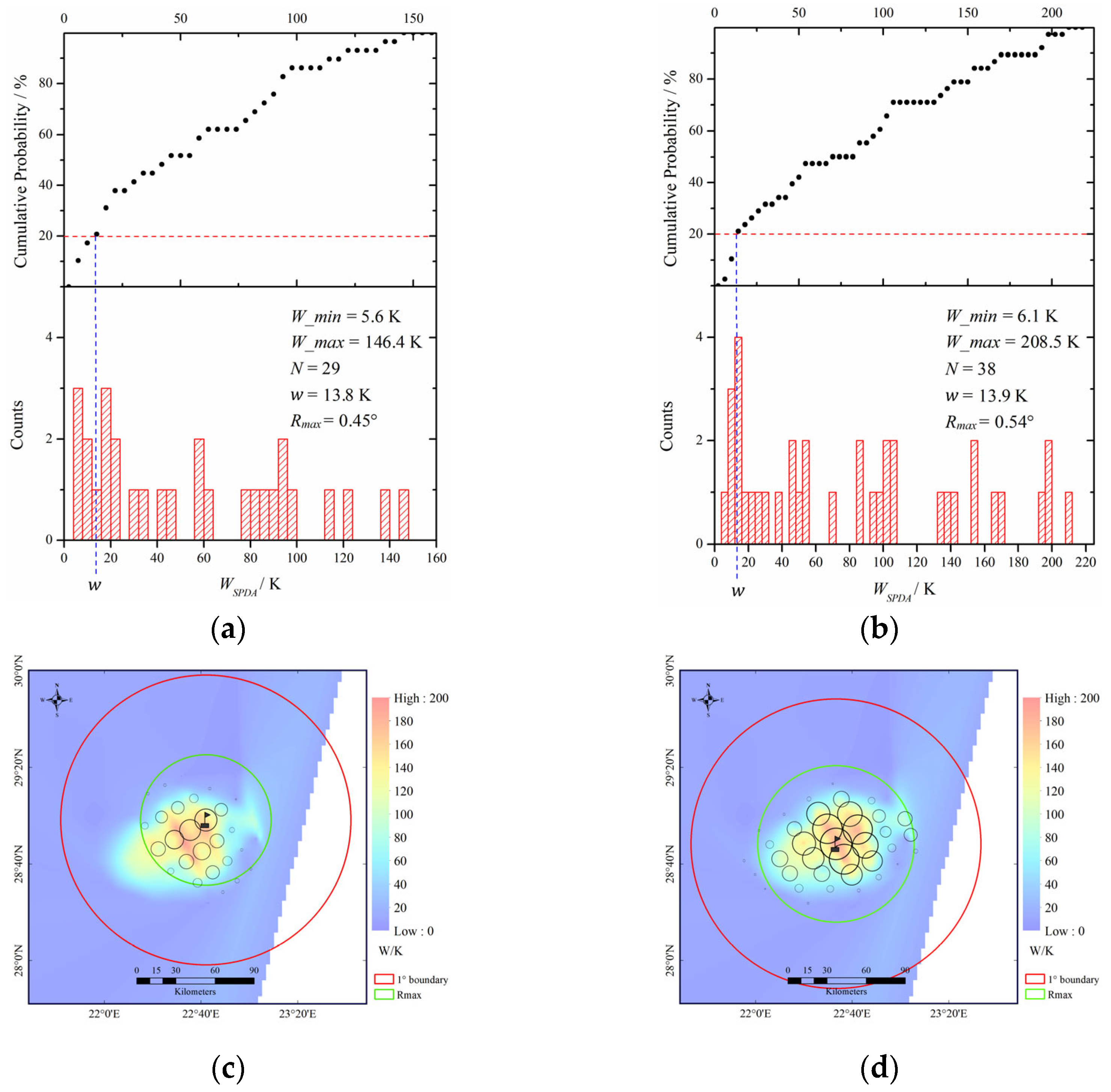
Determining Rmax entails statistically calculating the PDF and CDF (as detailed in Equation (7)) of WSPDA samples within a cluster. Figure 6 presents examples of statistical analysis for Rmax.
Based on the conducted statistical analysis for this study, a cumulative probability of 20% was established as an empirical constant. This constant serves to characterize the spatial distribution of the low values of WSPDA in a cluster. Following this, the corresponding value of w was determined through a statistical calculation using all extracted sample data. This value of w represents the upper boundary threshold for the WSPDA low-value zone within the cluster. Subsequently, the sample points with WSPDA values below w were identified. The distances from these samples to the point of Wmax within the cluster were then calculated, and a distance dataset Dedge was established. However, as can be discerned from the above discussion, if the minimum distance between two adjacent RFI source samples satisfies the classification condition of the DBSCAN method, these two RFI source samples will be clustered together. In the case that the clustering method possibly fails to fully distinguish between two adjacent RFI sources, there will be numerous abnormal low values of WSPDA. These values are obviously irrational and should not be used in subsequent calculations. Therefore, it is imperative to set a relatively rational boundary threshold based on experience. In this study, a threshold of 1° was selected.
A sample dataset of the low-value zone was established by summarizing the above boundary conditions, and averaging was conducted separately for the corresponding WSPDA and Dedge datasets in the sample dataset of low value to obtain values of parameters Wmean and Dmean, which characterize the samples at the cluster’s edge. The Dmean value was defined as the maximum action radius Rmax. As depicted in Figure 6, the selected Rmax is relatively rational, and it is a threshold that varies dynamically and can be adjusted automatically according to the emission intensity and influence range of different RFI sources.
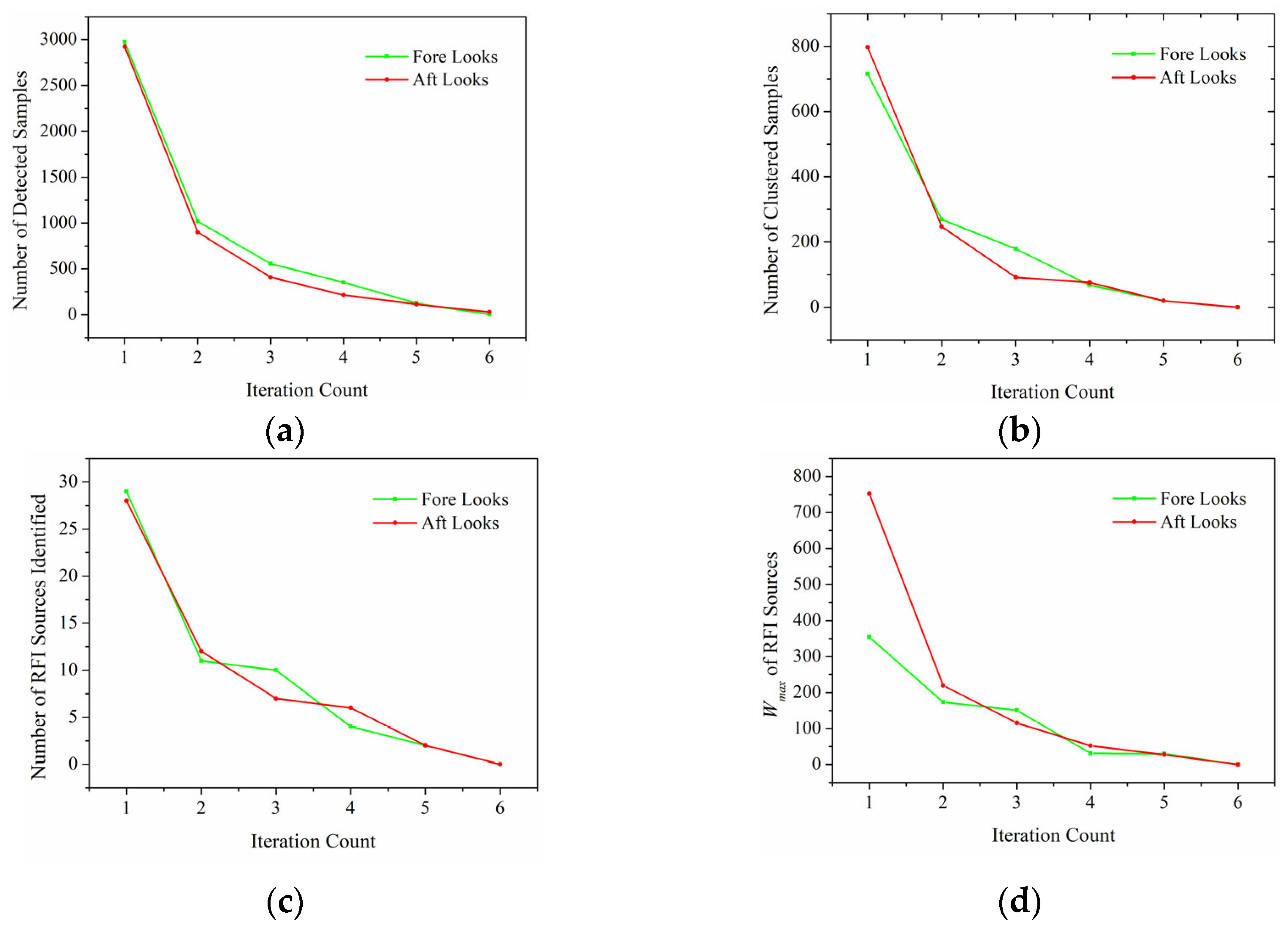
Figure 7 demonstrates the characteristics of the clustering identification results of the MICA-BEID algorithm as the number of iterations varies. It can be observed from the figure that for both fore and aft looks data, the number of detected samples, the number of clustered samples, the number of RFI sources identified through clustering, and the Wmax value of the RFI sources all peak in the initial iteration. With the increase in the number of iterations, these values exhibit a decreasing trend, and the variation characteristics for both fore and aft looks are essentially consistent. This indicates that the MICA-BEID algorithm is not only effective in detecting RFI sources but also capable of accurately identifying their different intensity levels.

3.2.3. Sidelobe Clusters Filtering

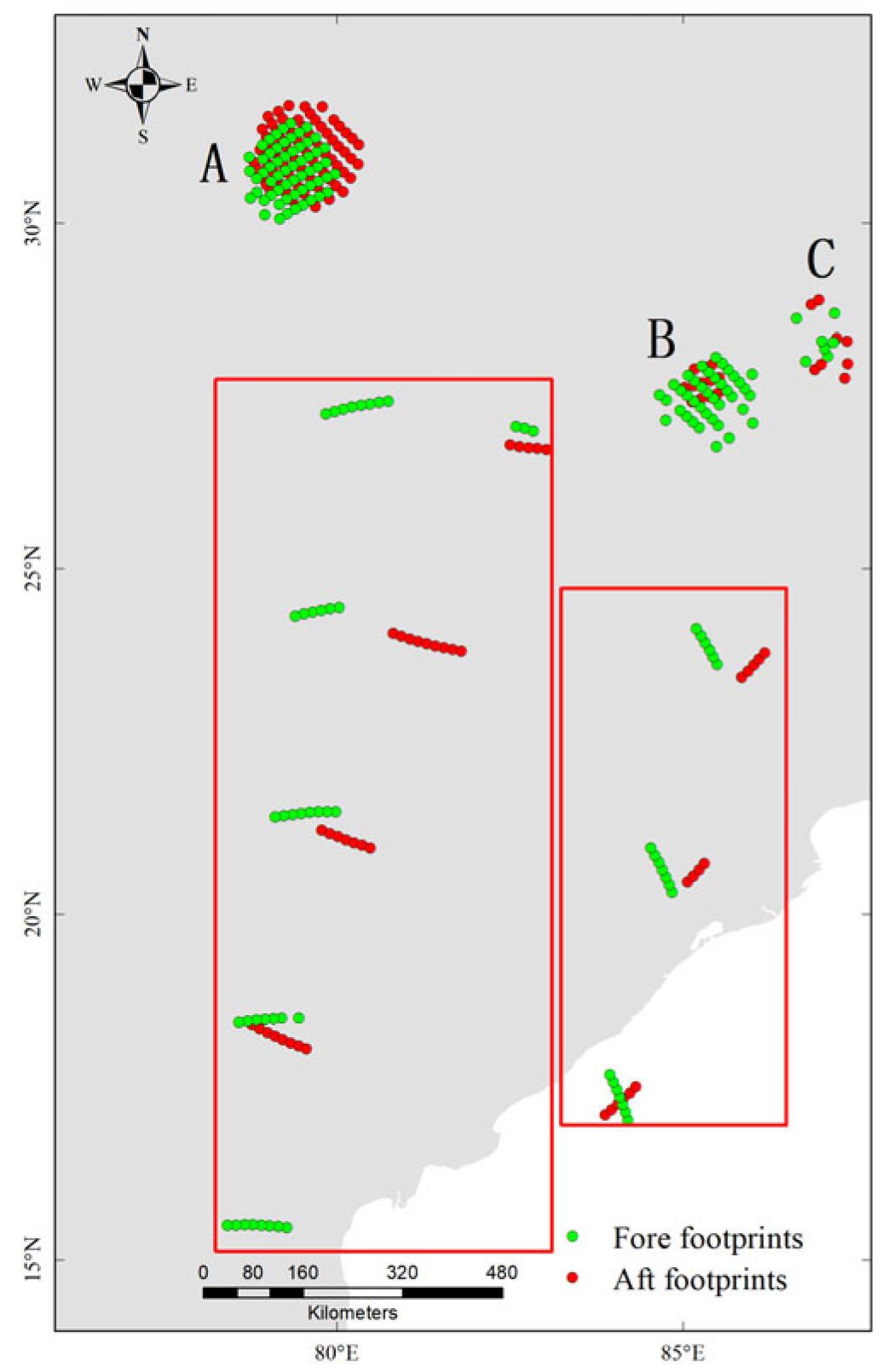
As there are numerous sidelobe clusters included in the initial clusters and they have relatively complex distribution characteristics, a sidelobe detection filtering algorithm was designed. The SMAP satellite operates on elliptical scanning orbits, which can be divided into fore and aft looks. As depicted in Figure 8, an RFI source generally influences multiple scanning orbits of fore and aft looks, with the influence being particularly evident at locations marked as A, B, and C. However, within the red-boxed area of the figure, there is a single scanning track for both the fore and aft looks footprints, which appears at regular intervals multiple times. This pattern may be caused through the sidelobes and it does not carry information on the location of the RFI source. Based on this characteristic, if a cluster contains two or fewer scanning orbits of fore or aft looks, the cluster is flagged as a sidelobe cluster and removed.

3.2.4. Water–Land Boundary Clusters Filtering

In this work, a filtering algorithm for water–land boundary clusters has been designed to address the limitations of conservative threshold increases. The case study’s statistical results presented in Table 2 and Figure 9 show that the presence of RFI sources increases the Wmax and the standard deviation within clusters at the water–land boundary. This indicates that RFI sources at the boundary are associated with a larger standard deviation. Consequently, the algorithm was designed to filter off clusters with a standard deviation below a certain threshold, which was empirically set to 4 K.

3.2.5. Faraday Rotation Clusters Filtering

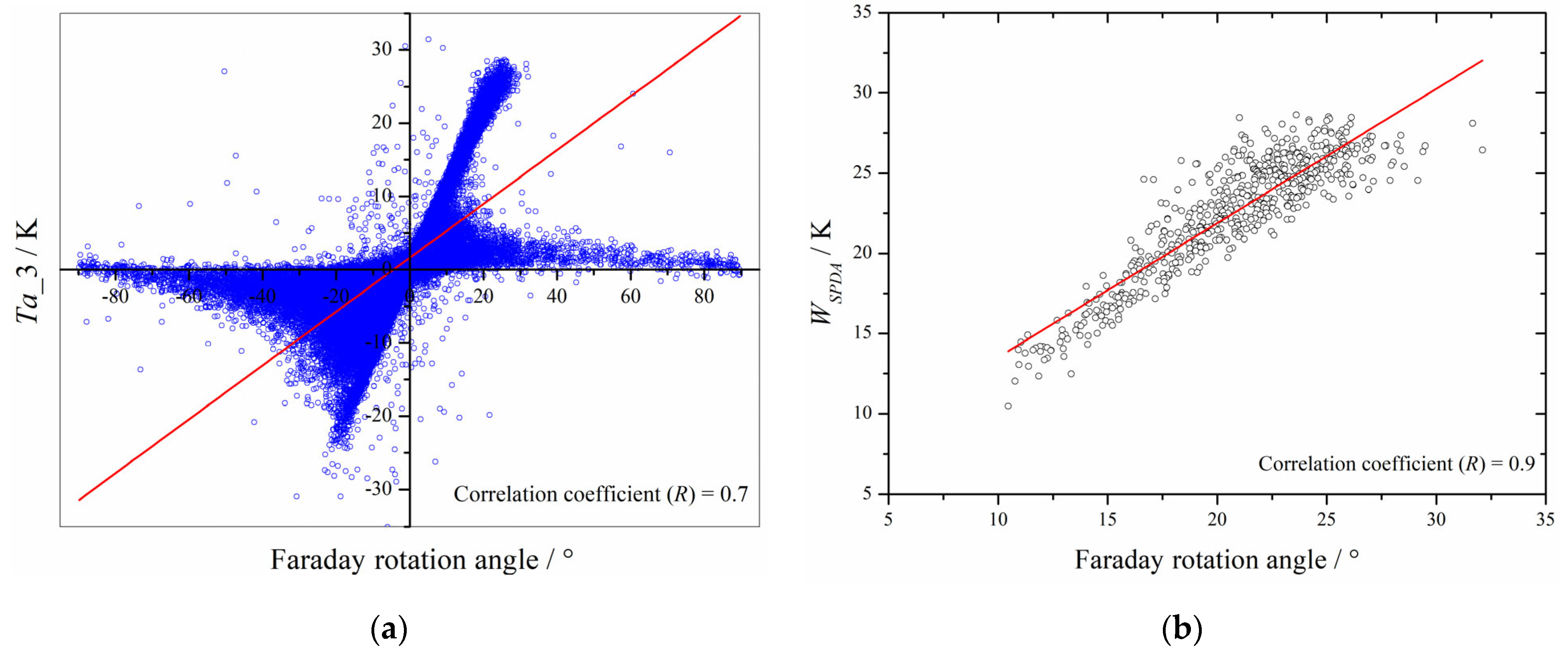
Faraday rotation affects the third Stokes parameter. Figure 10 shows a typical example of this effect, observed on February 27, 2023, during a period of high geomagnetic disturbance. The figure shows that Ta_3 of the SMAP satellite abnormally increased due to Faraday rotation, while Ta_4 was largely unaffected, leading to an overall increase in WSPDA. Figure 11 presents the results of the statistical analysis. Figure 11a is based on half-orbit data from the SMAP satellite, and Figure 11b utilizes the data specified within the blue box in the typical example. The analysis reveals a positive correlation between the Faraday rotation angle and Ta_3 within a range of 30 K. Within the blue box range in the typical example, there is a significant positive correlation between the Faraday rotation angle and WSPDA, with WSPDA varying between 10 and 30 K and a standard deviation of 3.7 K. Based on these characteristics, an empirical threshold of 4 K standard deviation was used to filter clusters affected by Faraday rotation.

3.3. Localization of RFI Sources

3.3.1. RFI Source Identification Algorithm

After systematic classification of RFI detection samples through iterative calculation, the RFI samples can be classified into numerous clusters by intensity based on the WSPDA values. Nevertheless, owing to the influences of multiple factors, the positions corresponding to satellite antennas obtained at abnormal temperatures do not align with the actual locations of RFI signal sources. In the RFI clustering process, some classified clusters have been removed through simple filtering. However, the filtering threshold is set in a too-conservative manner, and it fails to filter off all falsely classified clusters. Therefore, we need to establish an RFI identification algorithm according to the spatial distribution characteristics of the RFI sources’ impact on satellite-obtained data. This algorithm will help to determine whether there are RFI sources included in each cluster.
Figure 12 shows two- and three-dimensional intensity distributions of WSPDA in classified clusters. The red and black circles in Figure 12a represent fore and aft antenna scanning orbits, respectively. The size of each circle represents the magnitude of WSPDA intensity, and the main difference between fore and aft looks is the difference in the azimuth range. Figure 12b presents the corresponding three-dimensional distributions. Figure 12 illustrates that the impact of RFI sources on WSPDA’s spatial distribution characteristics is related to both azimuth and distance. The WSPDA’s intensity shows significant variation across different azimuths. Additionally, for a single antenna scanning orbit, the data from WSPDA suggest that RFI interference values decrease as the distance from the antenna scan footprints to the cluster’s Wmax location increases. Once this distance exceeds the Rmax threshold, WSPDA will not be affected by the RFI sources within the cluster.

3.3.2. Data Normalization

It can be seen from Figure 12 that, owing to the influences of dual factors, namely the pattern of the RFI source antennas and the satellite observation azimuth, the variation in satellite observation azimuth will cause evident differences in the integrated intensity of WSPDA between fore and aft looks of satellite antenna scanning orbits, which may result in relatively low values in medium- and strong-field zones of the RFI source and relatively high values in weak-field zones. In order to unify the WSPDA intensity of the fore and aft looks under a single standard for analysis, to provide a standardized sample dataset for machine learning, and to mitigate the potential impact of factors such as azimuth on the location results, we have normalized the data.
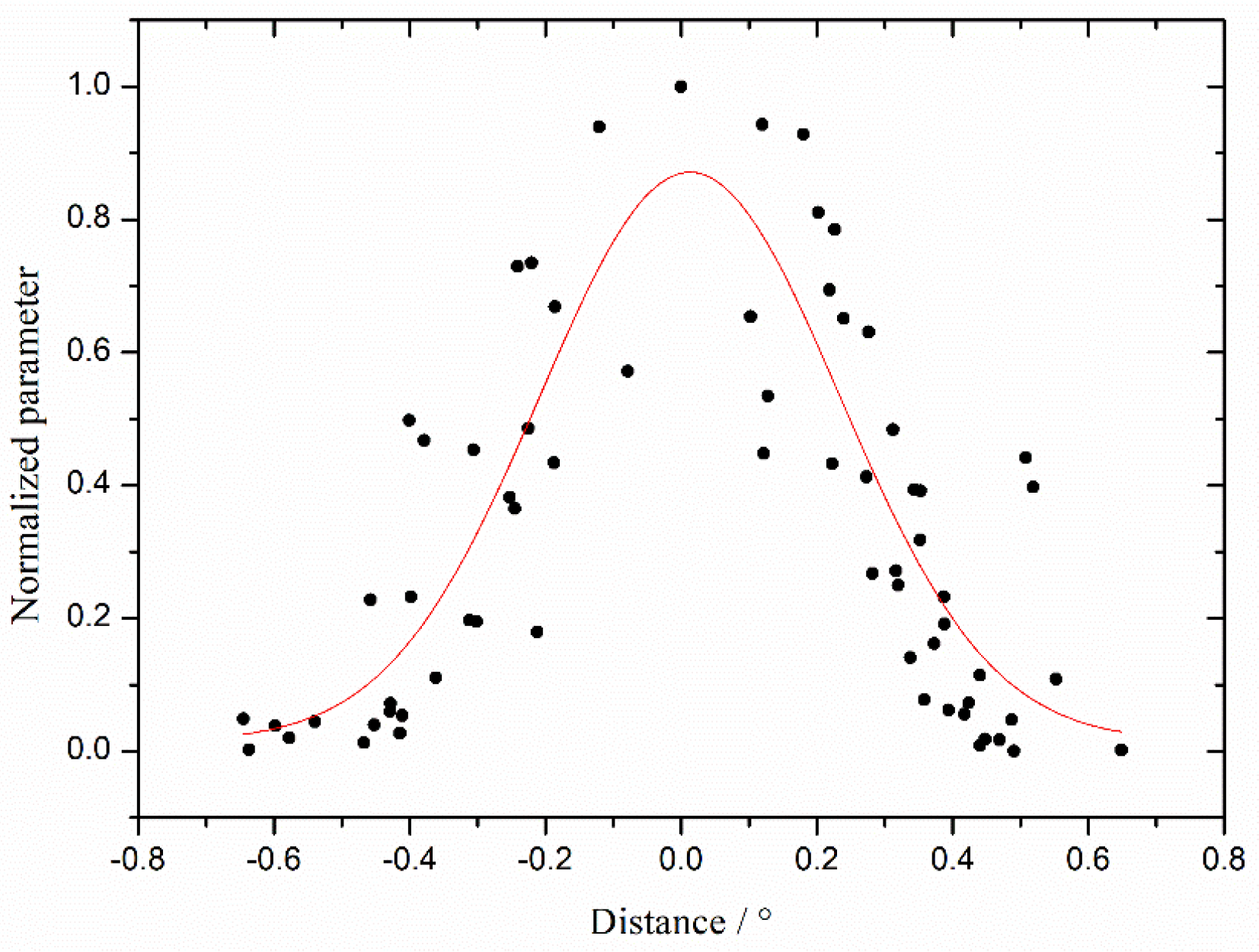
The dataset within a cluster was divided into two sub-datasets (i.e., fore and aft sub-datasets) based on the SMAP satellite antenna scanning direction (referred to as fore and aft looks). Then, the WSPDA intensity was normalized into the interval [0, 1] separately for these two sub-datasets using the normalization method. Afterward, these two sub-datasets were merged to establish a dataset of the normalized parameter and distance d and to establish a dataset of positive and negative distances with the longitude line at the Wmax in the cluster as the center line. Figure 13 shows statistical diagrams of the spatial distributions of the normalized parameter with distance. It can be seen from the figure that the distribution curves basically follow a Gaussian distribution.

3.3.3. Normalized Data Quality Control

Data normalization can eliminate the differences in the intensity level of WSPDA integrated intensity caused by different azimuths, but it is incapable of eliminating the differences in distance. Moreover, if multiple RFI sources are very close together, superposed interference may be formed. As can be discerned from Figure 12, it is possible that there may still be abnormal data in the dataset. This case mainly appears as low values in high-value zones and high values in low-value zones. These abnormal data need to be removed by data filtering. The specific method used was as follows: Initially, we established an RFI identification algorithm based on the spatial distribution characteristics. We set three action radii (i.e., R1, R2, and R3), with the Wmax point in the classified cluster as the center of the circle, out of which R3 is the maximum action radius Rmax of the RFI source. R1 and R2 were obtained through calculation with the following formulas:
R 1 = 1 3 R 3
R 2 = 2 3 R 3
We then established three sub-datasets ([0, R1], [R1, R2], and [R2, R3]) in the space range. We calculated the mean values of all normalized parameter values in the high-value zone [0, R1] and in the low-value zone [R2, R3], set thresholds h i g h and l o w , and removed abnormal data satisfying the following formulas:
W h i g h _ z o n e _ i h i g h < 0
W l o w _ z o n e _ j l o w > 0
to form a dataset after quality control. If a sample in the sub-dataset satisfied Equations (13) and (14), it was removed from the sub-dataset.

3.3.4. RFI Source Identification Results

After abnormal values were filtered off for each sub-dataset, the mean value was calculated for all sub-datasets (W1mean, W2mean, and W3mean). Based on the spatial distribution characteristics of the influence of RFI sources on the SMAP satellite, to finally determine whether there are RFI sources contained in the cluster, three sub-datasets in the cluster should meet the following criteria:
W 1 m e a n > W 2 m e a n > W 3 m e a n
If the classified cluster satisfies the above criteria, the position of the Wmax in the cluster was flagged as an RFI source. Figure 14 shows an example of conditions for the identification and determination of RFI as mentioned above. The red stars represent outlier data that have been removed, and the example meets the RFI identification and determination criteria.

3.3.5. Long-Time-Series Data Location of RFI Sources

Due to factors such as the radiation pattern of the RFI source, satellite observation azimuth, and satellite observation spatial resolution, a position obtained by a single-orbit location may not completely characterize the actual position of the RFI source. An RFI source location sample database was obtained from the RFI source location results based on long-time-series single-orbit data. Subsequent to this, secondary iterative clustering was conducted for the sample database to obtain an RFI identification cluster based on a long time series. To characterize the final location coordinates of the RFI source, the centroid of the RFI identification dataset was calculated with the following formula [14]:
L o c l o n / l a t = i n L o c _ i l o n / l a t W i i n W i
where L o c l o n / l a t represents the coordinates of the centroid in longitude and latitude, L o c _ i l o n / l a t represents the ith coordinates in longitude and latitude, and W i represents the ith synthesized parameter.
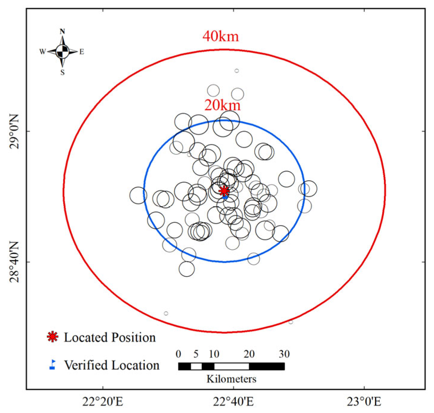
Figure 15 shows the long-time-series RFI source identification results from 1 January to 30 June 2017. It can be seen from the figure that, in the time period of half a year, the RFI identification and location exhibit some differences. However, the long-time-series RFI location data points are basically concentrated within an EFOV of the satellite antenna. The MICA-BEID algorithm, with confirmation from online satellite imagery, located a suspected RFI source, identified as a cellular tower in the Sahara Desert, approximately 1 km away.

4. Discussion

4.1. Information Carried by the Parameter WSPDA

In natural scenes, there is considerable variation in horizontal and vertical brightness temperatures, whereas the third and fourth Stokes parameters are expected to be small and nearly always zero. It is generally unlikely that artificial RFI sources will align with the polarimetric axes of L-band microwave radiometers, and thus, they are likely to contribute to the third and/or fourth Stokes parameters [27,28]. The new parameter, WSPDA, capitalizes on the low values of the third and fourth Stokes parameters. Anomalously high values of WSPDA can serve as effective indicators of RFI effects and have the potential to quantitatively describe the contributions from artificial RFI sources. Moreover, WSPDA is particularly sensitive to RFI, especially in detecting weak RFI signals.
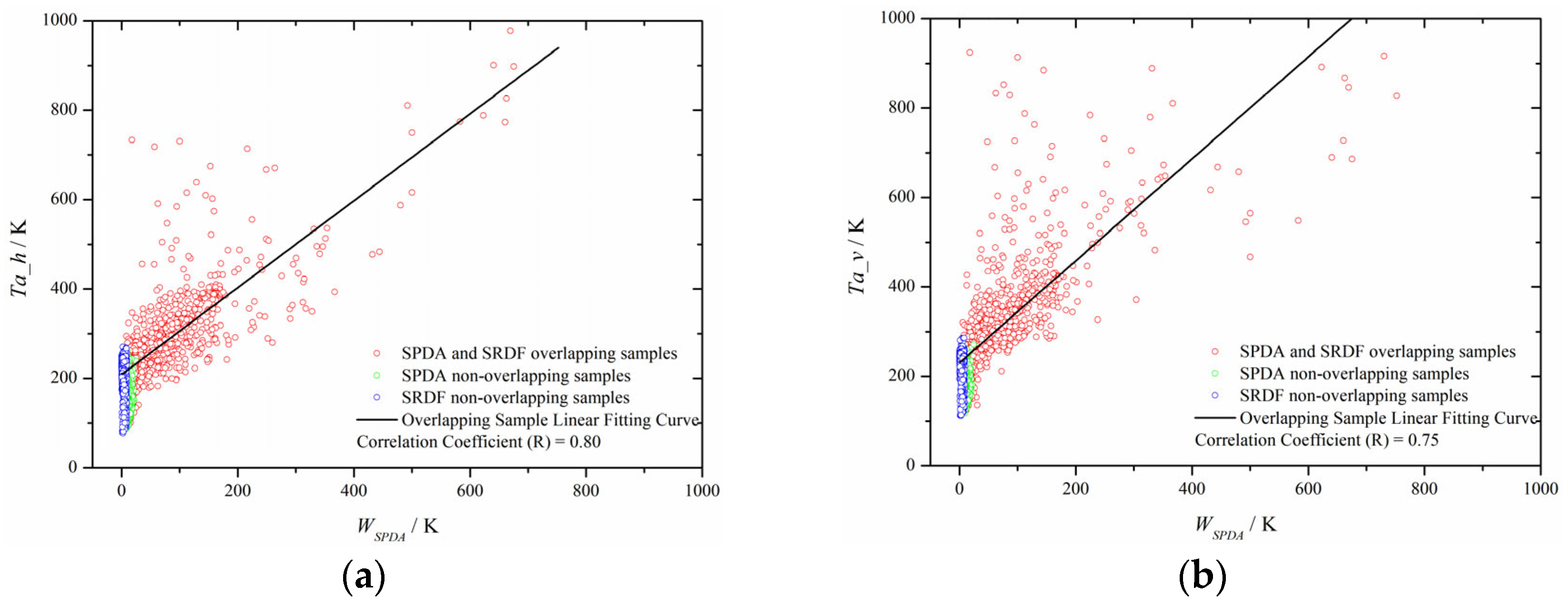
Figure 16 shows the characteristics of the relationship between WSPDA and the antenna temperatures for horizontal (Ta_h) and vertical (Ta_v) polarizations. As the figures indicate, WSPDA values in samples without overlap between SPDA and SRDF are mainly concentrated in the lower range from 0 to 20 K. Consistently, Ta_h and Ta_v remain within their natural range of levels. Conversely, in cases where SPDA and SRDF do overlap, WSPDA values show a broader distribution, from just above the detection threshold to 1000 K. The rise in WSPDA values corresponds to an increase in both Ta_h and Ta_v, indicating a significant positive correlation with the correlation coefficients of 0.8 and 0.75, respectively. This suggests that WSPDA can effectively characterize the extent of the impact of RFI sources on Ta_h and Ta_v, and it holds the potential for conducting quantitative analysis.

4.2. Comparison with the ITU’s RFI Survey Results

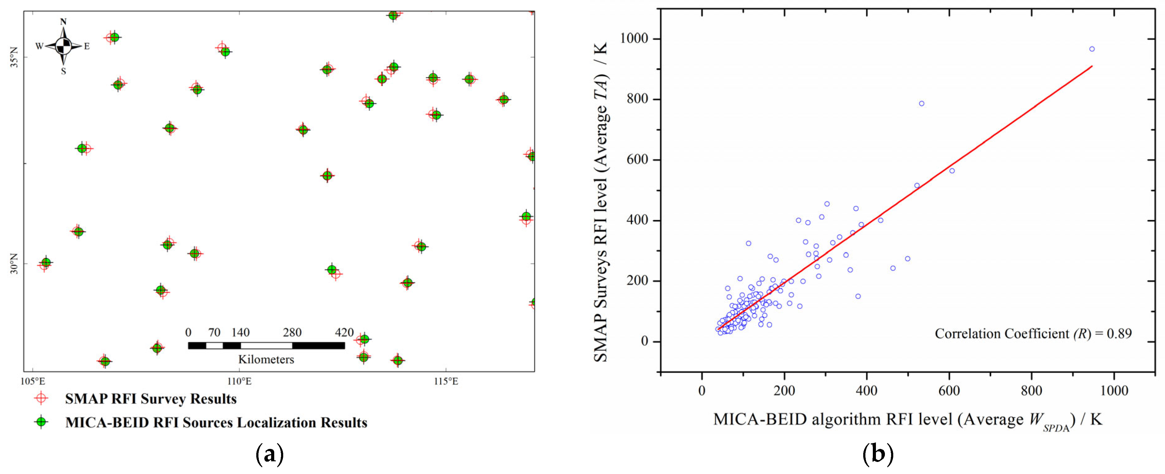
The ITU-R report presents global surveys of RFI levels observed by the SMAP L-band microwave radiometer in 2021. It employed a machine learning algorithm to localize the points where the effect of RFI is the highest [38]. Figure 17 shows the results of the comparative localization of RFI sources in local regions of China for October 2016. The analysis revealed that for 124 matching data sets, the localization distances were within 10 km, indicating a high degree of spatial consistency between the two sets of localization results. Furthermore, the interference intensity levels of the RFI sources localized by the two algorithms exhibit a significant positive correlation, with a correlation coefficient reaching 0.89. In summary, the comparative analysis suggests a high degree of consistency between the two algorithms regarding both the localization accuracy of RFI sources and the representation of RFI levels.

4.3. Comparison with Known Sources

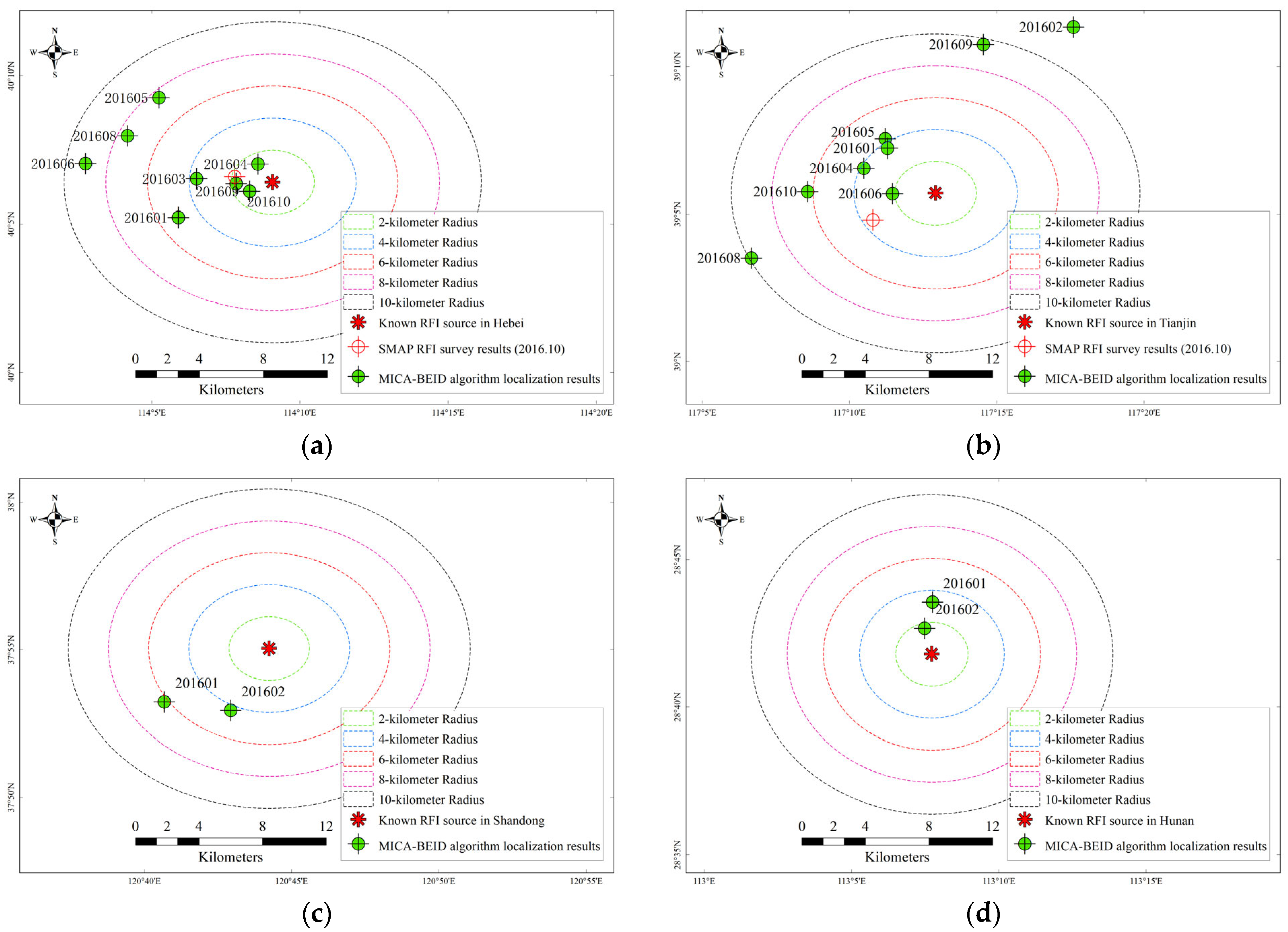
The known RFI sources are primarily based on information provided by the Radio Regulation of China. This information relates to RFI sources within the 1400–1427 MHz frequency band, which were investigated and subsequently turned off during the period of from 2016 to 2017 due to interference incidents. Table 3 presents a comparative analysis of localization results between the MICA-BEID algorithm and known RFI sources. Figure 18 illustrates the monthly spatiotemporal distribution of RFI source localization results over the extended period from January to October 2016.
From the figures and table, it is evident that the MICA-BEID algorithm is capable of identifying and localizing different types and levels of RFI sources, including broadcast and television towers, video surveillance equipment, and other microwave transmission antennas. Due to the different deactivation dates of these four RFI sources, both the MICA-BEID and SMAP RFI survey algorithms localized the sources in Hebei and Tianjin during October 2016. In Hebei, both algorithms achieved an approximate localization accuracy of 2 km, with the MICA-BEID algorithm showing a relatively better performance. In Tianjin, the MICA-BEID algorithm’s localization accuracy was approximately 6 km, while the SMAP RFI survey algorithm achieved higher accuracy with results at about 4 km. On a long-term scale, the monthly localization results from the MICA-BEID algorithm were distributed near the known RFI sources, with the majority within a 6 km range and the optimal localization accuracy reaching 1.2 km. After the RFI sources were manually turned off, the MICA-BEID algorithm stopped outputting localization results. This demonstrates that the MICA-BEID algorithm maintains stable localization performance and is capable of adapting well to changes in the status of RFI sources.

4.4. Comparison with SMOS

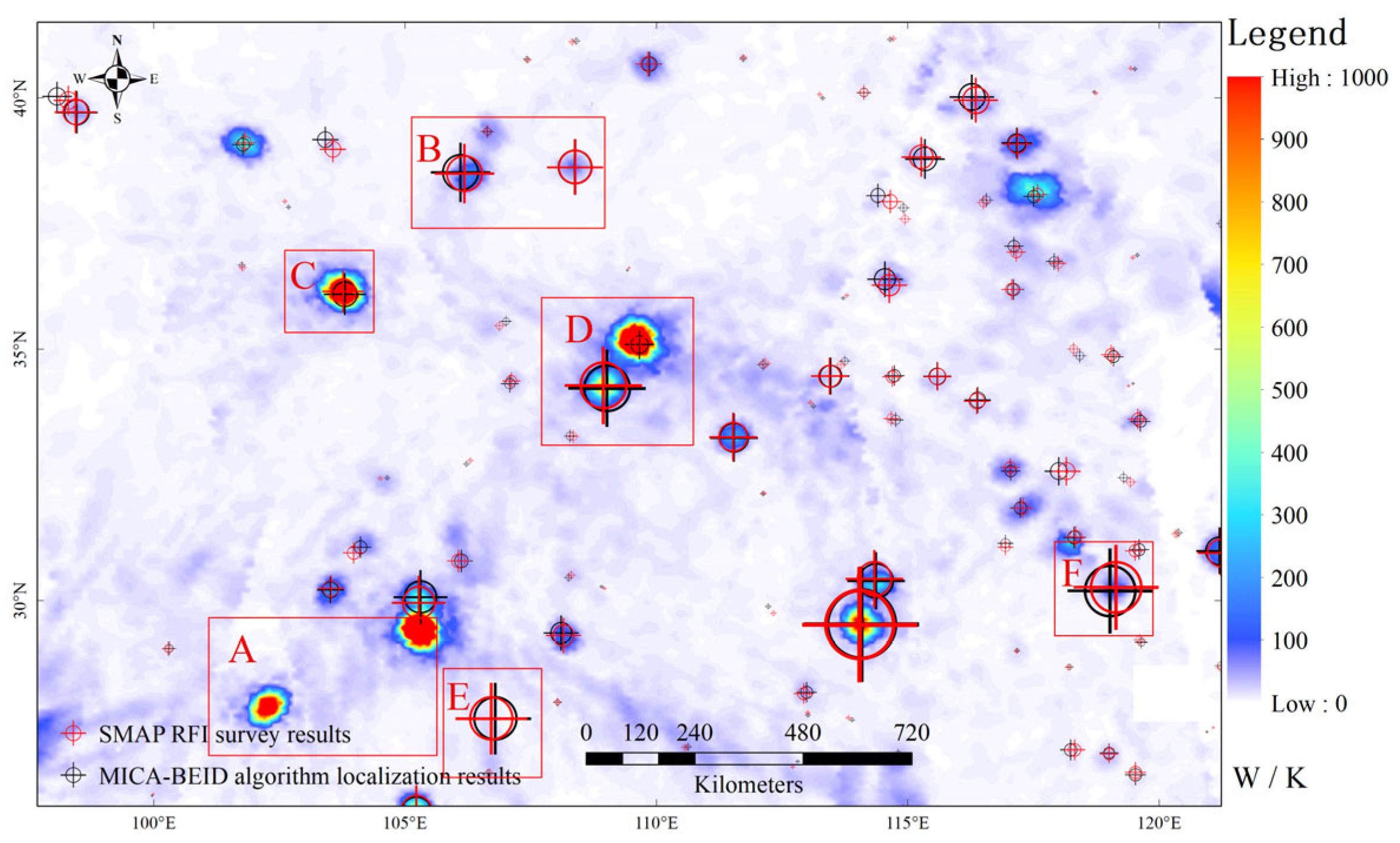
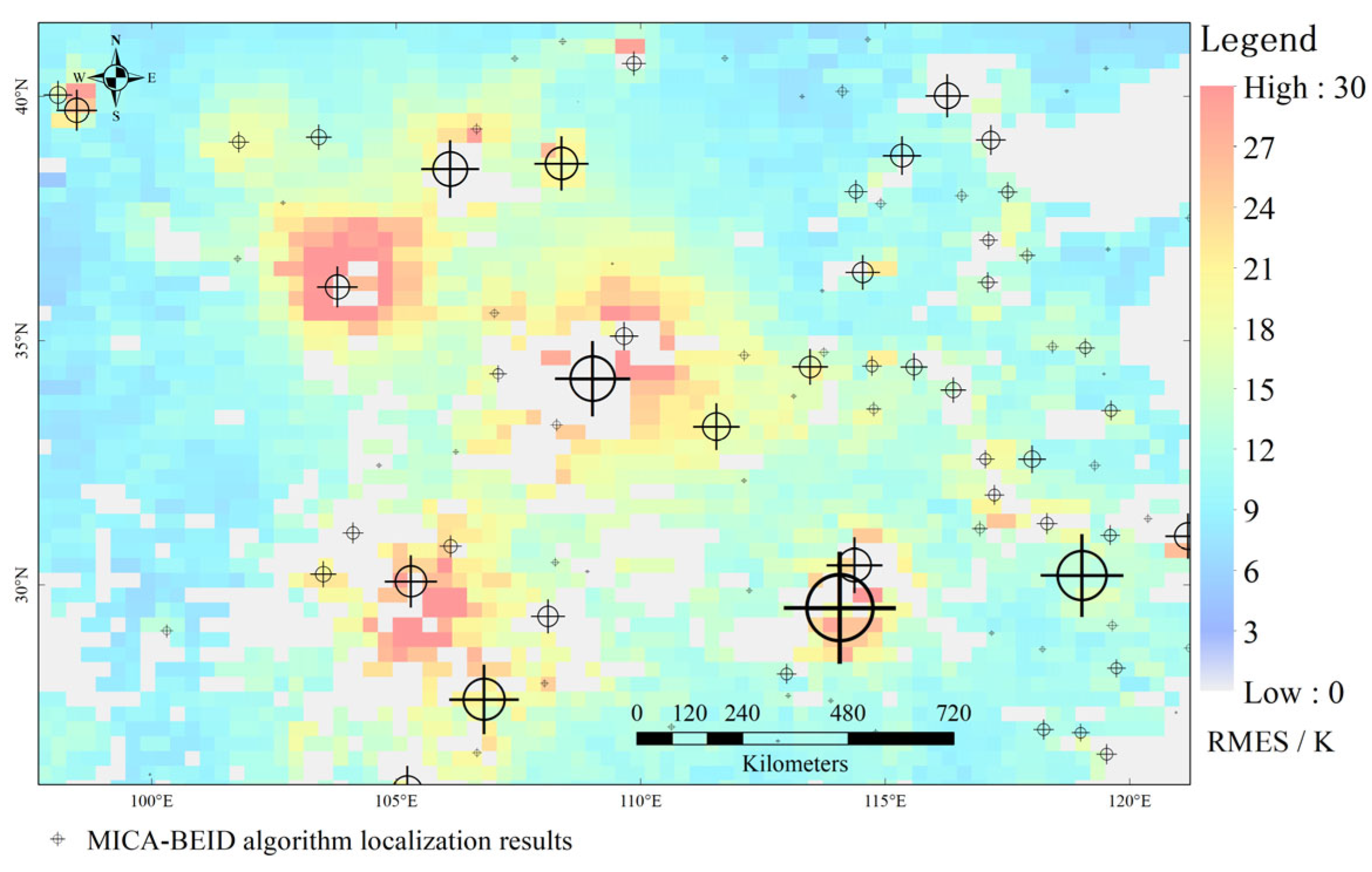
This paper utilized the SMOS satellite L1C (MIR_SCLF1C) data for October 2016, which covered China. The SNAP (Sentinel Applications Platform) 9.0.0 software was applied to produce spatial distribution maps of the WSPDA parameter, and the results were compared with those from the MICA-BEID and SMAP RFI survey algorithms. From Figure 19, it is evident that the RFI source localization results from the MICA-BEID algorithm largely align with the spatial distribution characteristics and the corresponding WSPDA levels of anomalies detected by the SMOS. Nonetheless, there are significant discrepancies in some areas, such as the one marked as Area A, where neither the MICA-BEID algorithm nor the SMAP RFI survey algorithm identified any RFI sources. Additionally, in Areas B, C, D, E, and F, there is a mismatch between the WSPDA levels from the SMOS and SMAP. These observations imply that the differences in the design and observational approaches of the L-band microwave radiometers on board the SMOS and SMAP satellites lead to unique responses to RFI. Furthermore, we also compared the RFI detection results with those obtained from the Root Mean Square Error (RMSE) method proposed by Wigneron et al. (2021). This algorithm estimates the impact of RFI on SMOS satellite brightness temperature data by calculating the RMSE between measured and modeled brightness temperatures [39]. Figure 20 presents a comparative chart that shows the monthly averaged brightness temperature RMSE (TB-RMSE) for October 2016, juxtaposed with the RFI localization results from the MICA-BEID algorithm. The comparison indicates that these two datasets have good spatial consistency.

5. Conclusions

In this paper, a polarization parameter named WSPDA was constructed using the SMAP antenna temperatures for the third and fourth Stokes parameters. With this parameter, a constrained iterative adaptive algorithm for RFI detection, clustering, identification, and localization, named MICA-BEID, was constructed using machine learning methods. It utilizes the WSPDA intensity and distribution density of RFI detection samples to enhance the identification and classification of RFI sources across various intensity levels.
The MICA-BEID algorithm was constructed based on the PDF and CDF of WSPDA. For RFI detection, the algorithm integrates the RFI detection samples based on dynamic thresholds of WSPDA and the original RFI flagged samples from the SMAP satellite, constructing a complementary dataset covering RFI sources of different intensities. In terms of the clustering of RFI detection samples, the algorithm takes the spatial distribution characteristics of WSPDA intensity and density in RFI detection samples into comprehensive consideration on the basis of the DBSCAN algorithm. It sets boundary conditions, such as the Rmax of RFI sources, using statistical methods. Through multiple iterations, the algorithm forms multiple effectively separable clusters. In terms of RFI source identification and localization, the algorithm identifies RFI sources based on the characteristic that the intensity of WSPDA samples diminishes as the distance increases from the location of Wmax and flags the WSPDA position within a cluster as the single localization result. Through secondary iterative clustering of single localization results on an extended time scale, the algorithm ultimately represents the localization results of RFI sources by the centroid position of the clusters.
Comprehensive assessment results indicate that the MICA-BEID algorithm has the capability to identify and localize RFI sources of various types and intensities and can adapt to their spatiotemporal changes. The algorithm exhibits good spatial consistency with other algorithms. Through cross-comparison analysis with known RFI sources on a long time scale, the optimal localization accuracy can reach approximately 1.2 km. The localization of RFI sources can guide relevant authorities in identifying illegal RFI sources, and it can accelerate the progress in turning off illegal RFI sources. Moreover, for RFI sources that cannot be turned off, the localization of RFI sources and the analysis of their long-time-series characteristics are important for simulating and constructing the spatial distribution characteristics of RFI source intensity.

Author Contributions

Conceptualization, X.W. (Xinxin Wang) and E.W.; methodology, X.W. (Xinxin Wang) and E.W.; software, X.W. (Xinxin Wang) and X.W. (Xiang Wang); validation, X.W. (Xinxin Wang); formal analysis, X.W. (Xinxin Wang); investigation, X.W. (Xinxin Wang) and J.F.; resources, X.W. (Xinxin Wang); data curation, X.W. (Xinxin Wang) and L.W.; writing—original draft preparation, X.W. (Xinxin Wang), X.W. (Xiang Wang), and E.W; writing—review and editing, X.W. (Xinxin Wang) and L.W.; visualization, X.W. (Xinxin Wang) and J.F.; supervision, X.W. (Xinxin Wang); project administration, X.W. (Xinxin Wang); funding acquisition, X.W. (Xinxin Wang). All authors have read and agreed to the published version of the manuscript.

Funding

This research was funded by the National Natural Science Foundation of China, Grant Number 41806212, and the National Key R&D Program of China, Grant Number 2016YFC1401000.

Data Availability Statement

The SMAP L1B_TB data for this paper are openly available at the National Snow and Ice Data Center (NSIDC) (https://nsidc.org/data/smap/data (accessed on 22 June 2021)). The SMOS L1C data for this paper are openly available at the European Space Agency (ESA) (https://smos-diss.eo.esa.int/oads/access/ (accessed on 2 March 2024)). The SMOS TB-RMSE data for this paper are openly available at https://ib.remote-sensing.inrae.fr (accessed on 7 May 2024).

Acknowledgments

The authors appreciate each open database for all the data provided: the NSIDC for the SMAP L1B_TB data, the ESA for the SMOS L1C data, the National Research Institute for Agriculture, Food and Environment(INRAE) for the SMOS TB-RMSE data. We would like to thank our reviewers for their comments and suggestions.

Conflicts of Interest

The authors declare no conflicts of interest.

References

  1. Salisbury, J.; Vandemark, D.; Joensson, B.; Balch, W.; Chakraborty, S.; Lohrenz, S.; Chapron, B.; Hales, B.; Mannino, A.; Mathis, J.T.; et al. How can present and future satellite missions support scientific studies that address ocean acidification? Oceanography 2015, 28, 108–121. [Google Scholar] [CrossRef]
  2. Entekhabi, D.; Njoku, E.G.; O’Neill, P.E.; Kellogg, K.H.; Crow, W.T.; Edelstein, W.N.; Entin, J.K.; Goodman, S.D.; Jackson, T.J.; Johnson, J.; et al. The Soil Moisture Active Passive (SMAP) Mission. Proc. IEEE 2010, 98, 704–716. [Google Scholar] [CrossRef]
  3. Tang, W.; Yueh, S.; Yang, D.; Fore, A.; Hayashi, A.; Lee, T.; Fournier, S.; Holt, B. The Potential and Challenges of Using Soil Moisture Active Passive (SMAP) Sea Surface Salinity to Monitor Arctic Ocean Freshwater Changes. Remote Sens. 2018, 10, 869. [Google Scholar] [CrossRef]
  4. Dinnat, E.P.; Le Vine, D.M.; Boutin, J.; Meissner, T. Satellite Sea Surface Salinity: Evaluation of Products and Impact of Retrieval Algorithms. In Proceedings of the IGARSS 2019—2019 IEEE International Geoscience and Remote Sensing Symposium, Yokohama, Japan, 28 July–2 August 2019; pp. 7936–7939. [Google Scholar] [CrossRef]
  5. Fore, A.; Yueh, S.; Tang, W.; Hayashi, A. The JPL SMAP Sea Surface Salinity Algorithm. In Proceedings of the IGARSS 2019—2019 IEEE International Geoscience and Remote Sensing Symposium, Yokohama, Japan, 28 July–2 August 2019; pp. 7920–7923. [Google Scholar] [CrossRef]
  6. Klein, L.; Swift, C. An Improved Model for the Dielectric Constant of Sea Water at Microwave Frequencies. IEEE Trans. Antennas Propag. 1977, 25, 104–111. [Google Scholar] [CrossRef]
  7. Yueh, S.H.; West, R.; Wilson, W.J.; Li, F.K.; Njoku, E.G.; Rahmat-Samii, Y. Error sources and feasibility for microwave remote sensing of ocean surface salinity. IEEE Trans. Geosci. Remote Sens. 2001, 39, 1049–1060. [Google Scholar] [CrossRef]
  8. Toose, P.; Roy, A.; Solheim, F.; Derksen, C.; Royer, A.; Walker, A. Radio frequency interference mitigating hyperspectral L-band radiometer. Geosci. Instrum. Method Data Syst. 2017, 6, 39–51. [Google Scholar] [CrossRef]
  9. Oliva, R.; Daganzo, E.; Kerr, Y.H.; Mecklenburg, S.; Nieto, S.; Richaume, P.; Gruhier, C. SMOS Radio Frequency Interference Scenario: Status and Actions Taken to Improve the RFI Environment in the 1400–1427-MHz Passive Band. IEEE Trans. Geosci. Remote Sens. 2012, 50, 1427–1439. [Google Scholar] [CrossRef]
  10. Le Vine, D.M.; de Matthaeis, P.; Ruf, C.S.; Chen, D.D. Aquarius RFI detection and mitigation algorithm: Assessment and examples. IEEE Trans. Geosci. Remote Sens. 2013, 52, 4574–4584. [Google Scholar] [CrossRef]
  11. Mohammed, P.N.; Aksoy, M.; Piepmeier, J.R.; Johnson, J.T.; Bringer, A. SMAP L-band microwave radiometer: RFI mitigation prelaunch analysis and first year on-orbit observations. IEEE Trans. Geosci. Remote Sens. 2016, 54, 6035–6047. [Google Scholar] [CrossRef]
  12. Soldo, Y.; Le Vine, D.M.; de Matthaeis, P.; Richaume, P. L-Band RFI Detected by SMOS and Aquarius. IEEE Trans. Geosci. Remote Sens. 2017, 55, 4220–4235. [Google Scholar] [CrossRef]
  13. Llorente, A.; Daganzo, E.; Oliva, R.; Uranga, E.; Kerr, Y.; Richaume, P.; de la Fuente, A.; Martin-Neira, M.; Mecklenburg, S. Lessons Learnt from SMOS RFI Activities after 10 Years in Orbit: RFI Detection and Reporting to Claim Protection and Increase Awareness of the Interference Problem in the 1400–1427 MHZ Passive Band. In Proceedings of the 2019 RFI Workshop—Coexisting with Radio Frequency Interference (RFI), Toulouse, France, 23–26 September 2019; pp. 1–6. [Google Scholar] [CrossRef]
  14. Soldo, Y.; Le Vine, D.M.; Bringer, A.; de Matthaeis, P.; Oliva, R.; Johnson, J.T.; Piepmeier, J.R. Location of Radio-Frequency Interference Sources Using the SMAP L-Band Radiometer. IEEE Trans. Geosci. Remote Sens. 2018, 56, 6854–6866. [Google Scholar] [CrossRef]
  15. Dinnat, E.; Le Vine, D. L-band radiometer calibration consistency assessment for the SMOS, SMAP and Aquarius instruments. In Proceedings of the 2016 IEEE International Geoscience and Remote Sensing Symposium (IGARSS), Beijing, China, 10–15 July 2016; pp. 2047–2049. [Google Scholar] [CrossRef]
  16. Camps, A.; Gourrion, J.; Tarongí, J.; Vall-llossera, M.; Gutierrez, A.; Castro, J.B.Y.R. Radio-Frequency Interference Detection and Mitigation Algorithms for Synthetic Aperture Radiometers. Algorithms 2011, 4, 155–182. [Google Scholar] [CrossRef]
  17. Johnson, J.T.; Mohammed, P.N.; Piepmeier, J.R.; Bringer, A.; Aksoy, M. Soil Moisture Active Passive (SMAP) Microwave Radiometer Radio-Frequency Interference (RFI) Mitigation: Algorithm Updates and Performance Assessment. In Proceedings of the 2016 IEEE International Geoscience and Remote Sensing Symposium (IGARSS), Beijing, China, 10–15 July 2016; pp. 123–124. [Google Scholar] [CrossRef]
  18. Piepmeier, J.R.; Johnson, J.T.; Mohammed, P.N.; Bradley, D.; Ruf, C.; Aksoy, M.; Garcia, R.; Hudson, D.; Miles, L.; Wong, M. Radio-Frequency Interference Mitigation for the Soil Moisture Active Passive Microwave Radiometer. IEEE Trans. Geosci. Remote Sens. 2013, 52, 761–775. [Google Scholar] [CrossRef]
  19. Aksoy, M. Radio Frequency Interference Characterization and Detection in L-Band Microwave Radiometry. Ph.D. Thesis, The Ohio State University, Columbus, OH, USA, 2015. [Google Scholar]
  20. Piepmeier, J.R.; Focardi, P.; Horgan, K.A.; Knuble, J.; Ehsan, N.; Lucey, J. SMAP L-band microwave radiometer: Instrument design and first year on orbit. IEEE Trans. Geosci. Remote Sens. 2017, 55, 1954–1966. [Google Scholar] [CrossRef]
  21. Nazar, I.M.; Aksoy, M. Radio Frequency Interference detection in microwave radiometry using Multi–Dimensional Semi Supervised Learning. In Proceedings of the IGARSS 2023–2023 IEEE International Geoscience and Remote Sensing Symposium, Pasadena, CA, USA, 16–21 July 2023; pp. 589–591. [Google Scholar] [CrossRef]
  22. Owfi, A.; Afghah, F. Autoencoder-based radio frequency interference mitigation for SMAP passive radiometer. In Proceedings of the IGARSS 2023-2023 IEEE International Geoscience and Remote Sensing Symposium, Pasadena, CA, USA, 16–21 July 2023; pp. 6783–6786. [Google Scholar] [CrossRef]
  23. Wang, X.X.; Wang, X.; Han, Z.; Yang, J.H. Radio Frequency Interference Detection and Characteristic Analysis Based on the L Band Stokes Parameters Remote Sensing Data. JEIT 2015, 37, 2342–2348. [Google Scholar] [CrossRef]
  24. Yang, Y.; Zhang, J.; Bao, Z.; Ao, T.; Wang, G.; Wu, H.; Wang, J. Evaluation of Multi-Source Soil Moisture Datasets over Central and Eastern Agricultural Area of China Using In Situ Monitoring Network. Remote Sens. 2021, 13, 1175. [Google Scholar] [CrossRef]
  25. Gabarró, P.C. Study of Salinity Retrieval Errors for the SMOS Mission. Ph.D. Thesis, University Politècnica de Catalunya, Barcelona, Spain, 2004. [Google Scholar]
  26. Yin, X.B. A Study on the Passive Microwave Remote Sensing of Sea Surface Wind Vector, Temperature and Salinity and the Effect of Wind on Remote Sensing of Temperature and Salinity. Ph.D. Thesis, Ocean University of China, Qingdao, China, 2007. [Google Scholar]
  27. Pardé, M.; Zribi, M.; Fanise, P.; Dechambre, M. Analysis of RFI Issue Using the CAROLS L-Band Experiment. IEEE Trans. Geosci. Remote Sens 2011, 49, 1063–1070. [Google Scholar] [CrossRef]
  28. Kristensen, S.S.; Balling, J.E.; Skou, N.; Søbjærg, S.S. RFI detection in SMOS data using 3rd and 4th Stokes parameters. In Proceedings of the 2012 12th Specialist Meeting on Microwave Radiometry and Remote Sensing of the Environment (MicroRad), Rome, Italy, 5–9 March 2012; pp. 1–4. [Google Scholar] [CrossRef]
  29. Soldo, Y.; Le Vine, D.M.; Dinnat, E. SMAP Observations of the Fourth Stokes Parameter At L-Band. In Proceedings of the IGARSS 2019—2019 IEEE International Geoscience and Remote Sensing Symposium, Yokohama, Japan, 28 July–2 August 2019; pp. 8407–8410. [Google Scholar] [CrossRef]
  30. Hartmann, J.; Habersack, J.; Steiner, H.J. Accurate and Efficient Satellite Payload Testing in Compact Ranges. In Proceedings of the 28th ESA Antenna Workshop on Space Antenna Systems and Technologies, Noordwijk, The Netherlands, 31 May–3 June 2005. [Google Scholar]
  31. Recommendation ITU-R RS.2106-0. Detection and Resolution of Radio Frequency Interference to Earth Exploration-Satellite Service (Passive) Sensors. (07/2017), RS Series, Remote Sensing Systems. Posted on 12 March 2017. Available online: https://www.itu.int/rec/R-REC-RS.2106-0-201707-I (accessed on 1 April 2024).
  32. Aksoy, M.; Rajabi, H.; Atrey, P.; Mohamed Nazar, I. Characteristics of the Global Radio Frequency Interference in the Protected Portion of L-Band. Remote Sens. 2021, 13, 253. [Google Scholar] [CrossRef]
  33. Fournier, S.; Bingham, F.M.; González-Haro, C.; Hayashi, A.; Ulfsax Carlin, K.M.; Brodnitz, S.K.; González-Gambau, V.; Kuusela, M. Quantification of Aquarius, SMAP, SMOS and Argo-Based Gridded Sea Surface Salinity Product Sampling Errors. Remote Sens. 2023, 15, 422. [Google Scholar] [CrossRef]
  34. Soldo, Y.; Cabot, F.; Khazaal, A.; Miernecki, M.; Slominska, E.; Fieuzal, R.; Kerr, Y.H. Localization of RFI sources for the SMOS mission: A means for assessing SMOS pointing performances. IEEE J. Sel. Top. Appl. Earth Obs. Remote Sens. 2015, 8, 617–627. [Google Scholar] [CrossRef]
  35. Corbella, I.; Martin-Neira, M.; Oliva, R.; Torres, F.; Duffo, N. Reduction of Secondary Lobes in Aperture Synthesis Radiometry. IEEE Geosci. Remote Sens. Lett. 2012, 9, 977–979. [Google Scholar] [CrossRef]
  36. Ester, M.; Kriegel, H.-P.; Sander, J.; Xu, X. A Density-Based Algorithm for Discovering Clusters in Large Spatial Databases with Noise. In Proceedings of the 2nd International Conference on Knowledge Discovery and Data Mining (KDD-96), Portland, OR, USA, 2–4 August 1996; pp. 226–231. [Google Scholar]
  37. Entekhabi, D.; Yueh, S.; O’Neill, P.E.; Kellogg, K.H.; Allen, A.; Bindlish, R.; Brown, M.; Chan, S.; Colliander, A.; Crow, W.T.; et al. SMAP Handbook–Soil Moisture Active Passive: Mapping Soil Moisture and Freeze/Thaw from Space; JPL Publication: Pasadena, CA, USA, 2014.
  38. Report ITU-R RS.2491-0; Global Survey of Radio Frequency Interference Observed by the SMAP Radar in the 1215 to 1300 MHz Band and the SMAP Radiometer in the 1400 to 1427 MHz Band. International Telecommunications Union, 2021; ITU RS Series, Remote Sensing Systems. Posted on September 2021. Available online: https://www.itu.int/pub/R-REP-RS.2491 (accessed on 2 April 2024).
  39. Wigneron, J.-P.; Li, X.; Frappart, F.; Fan, L.; Al-Yaari, A.; De Lannoy, G.; Liu, X.; Wang, M.; Le Masson, E.; Moisy, C. SMOS-IC data record of soil moisture and L-VOD: Historical development, applications and perspectives. Remote Sens. Environ. 2021, 254, 112238. [Google Scholar] [CrossRef]
Figure 1. Flowchart for the constrained iterative adaptive algorithm.
Remotesensing 16 01791 g001
Figure 2. Statistical histogram of calculation results of SMAP L1B half-orbit data parameter WSPDA for (a) the ascending orbit and (b) the descending orbit.
Remotesensing 16 01791 g002
Figure 3. Spatial distribution of SMAP RFI detection sample data. (a,b) RFI detection samples inside (green) and on the edges (red) of the ascending and descending orbits, respectively; (c,d) SMAP RFI SRDF samples (blue), SPDA samples (red) and overlapped samples (green) in ascending and descending orbits, respectively, with the samples on the edges being removed.
Remotesensing 16 01791 g003aRemotesensing 16 01791 g003b
Figure 4. Local spatial distribution of SMAP RFI detection sample data at the water–land boundary. The background is the spatial interpolation results of WSPDA. The detection results of the descending orbit at a detection threshold of 5.5 K are in red, and those at a detection threshold of 9.3 K are in green.
Remotesensing 16 01791 g004
Figure 5. Spatial distribution of RFI detection samples after interpolation for (a) land only and (b) at the water–land boundary.
Remotesensing 16 01791 g005
Figure 6. Rmax statistical analysis examples. (a,b) Statistical results of RFI detection samples for fore and aft looks, respectively; (c,d) spatial distribution of WSPDA intensity of clusters for fore and aft looks, respectively. The background is the spatial interpolation results of WSPDA for all fore and aft detection samples.
Remotesensing 16 01791 g006
Figure 7. The changing characteristics of clustering identification results with iteration count. (a) Number of detected samples; (b) number of clustered samples; (c) number of RFI sources identified; (d) Wmax of RFI sources.
Remotesensing 16 01791 g007
Figure 8. Spatial distribution of RFI detection samples for the SMAP satellite’s fore and aft looks footprints.
Remotesensing 16 01791 g008
Figure 9. Filtering results of clusters at the water–land boundary. (a) All clustering results for all samples, where various colors denote different clusters; (b) results of cluster filtering, with red indicating the removed clusters and green indicating the retained clusters.
Remotesensing 16 01791 g009
Figure 10. A typical example of the effects of Faraday rotation during a period of high geomagnetic disturbance on 27 February 2023.
Remotesensing 16 01791 g010
Figure 11. Statistical analysis results of the impact of Faraday rotation. (a) Data from half-orbit of the SMAP satellite. (b) Data within the blue box range, as depicted in Figure 10, of a typical example. The red line in both (a) and (b) represents the result of linear fitting.
Remotesensing 16 01791 g011
Figure 12. (a) Two- and (b) three-dimensional intensity distributions of WSPDA of clusters for descending orbit. Red and black circles represent fore and aft antenna scanning orbits, respectively.
Remotesensing 16 01791 g012
Figure 13. Statistical diagrams of spatial distribution of the normalized parameter with distance for descending orbits.
Remotesensing 16 01791 g013
Figure 14. RFI identification and determination criteria. The red stars represent outlier data that have been removed.
Remotesensing 16 01791 g014
Figure 15. Spatial distribution characteristic of long-time-series RFI location data points and the RFI location centroid.
Remotesensing 16 01791 g015
Figure 16. The characteristics of the relationship between the WSPDA parameter and the antenna temperatures for (a) horizontal (Ta_h) and (b) vertical (Ta_v) polarizations.
Remotesensing 16 01791 g016
Figure 17. Comparison results between MICA-BEID algorithm and SMAP RFI surveys. (a) Comparison of RFI location results; (b) comparison of RFI levels.
Remotesensing 16 01791 g017
Figure 18. Comparative analysis of MICA-BEID algorithm RFI localization results with known RFI sources on a long-term scale. (a) Hebei. (b) Tianjin. (c) Shandong. (d) Hunan.
Remotesensing 16 01791 g018
Figure 19. Comparative analysis of RFI localization results with MICA-BEID algorithm with WSPDA of the SMOS satellite.
Remotesensing 16 01791 g019
Figure 20. Comparative analysis of RFI localization results with MICA-BEID algorithm with the average TB-RMSE.
Remotesensing 16 01791 g020
Table 1. RFI detection results based on SMAP L1B half-orbit data (ascending and descending orbits).
OrbitTotal Number of RFI Detection SamplesNumber of Samples on Orbit EdgeNumber of
Samples inside Orbit
Number of SRDF Samples inside OrbitNumber of SPDA Samples inside OrbitNumber of
Overlapped Samples
Ascending15,231380611,425743678533864
Descending 14,44645259921491576082602
Table 2. Statistical results of clustering for RFI detection samples at water–land boundary.
ClustersMinimum Value (K)Maximum Value (K)Standard Deviation (K)Number of Samples
A9.9216.276.380
B9.918.72.2112
C10.1366.7115.154
D9.821.73.1108
E9.8212.6131
Table 3. Comparative analysis of statistical results with known RFI sources.
RegionOptimal Location Distance (km)Wmax (K)Types of Known RFI SourcesDate Turned Off
Hebei1.2200.4Broadcast and television tower2017-08
Tianjin2.1434.7Video surveillance equipment.2017-08
Shandong3.8959.1Broadcast and television tower2016-03
Hunan1.71340.7Microwave transmission antenna2016-03
Disclaimer/Publisher’s Note: The statements, opinions and data contained in all publications are solely those of the individual author(s) and contributor(s) and not of MDPI and/or the editor(s). MDPI and/or the editor(s) disclaim responsibility for any injury to people or property resulting from any ideas, methods, instructions or products referred to in the content.