Article

Optimizing the Numerical Simulation of the Dust Event of March 2021: Integrating Aerosol Observations through Multi-Scale 3D Variational Assimilation in the WRF-Chem Model

1
College of Meteorology and Oceanography, National University of Defense Technology, Changsha 410073, China
2
College of Advanced Interdisciplinary Studies, National University of Defense Technology, Changsha 410073, China
3
State Key Laboratory of Severe Weather, Chinese Academy of Meteorological Sciences, Beijing 100081, China
*
Author to whom correspondence should be addressed.
Remote Sens. 2024, 16(11), 1852; https://doi.org/10.3390/rs16111852
Submission received: 23 April 2024 / Revised: 17 May 2024 / Accepted: 18 May 2024 / Published: 22 May 2024
(This article belongs to the Section Atmospheric Remote Sensing)

Abstract

:
The integration of high-resolution aerosol measurements into an atmospheric chemistry model can improve air quality forecasting. However, traditional data assimilation methods are challenged in effectively incorporating such detailed aerosol information. This study utilized the WRF-Chem model to conduct data assimilation and prediction experiments using the Himawari-8 satellite’s aerosol optical depth (AOD) product and ground-level particulate matter concentration (PM) measurements during a record-breaking dust event in the Beijing–Tianjin–Hebei region from 14 to 18 March 2021. Three experiments were conducted, comprising a control experiment without assimilation (CTL), a traditional three-dimensional variational (3DVAR) experiment, and a multi-scale three-dimensional variational (MS-3DVAR) experiment. The results indicated that the CTL method significantly underestimated the intensity and extent of the severe dust event, while the analysis fields and forecasting fields of PM concentration and AOD can be significantly improved in both 3DVAR and MS-3DVAR assimilation. Particularly, the MS-3DVAR assimilation approach yielded better-fitting extreme values than the 3DVAR method, mostly likely due to the multi-scale information from the observations used in the MS-3DVAR method. Compared to the CTL method, the correlation coefficient of MS-3DVAR assimilation between the assimilated PM10 analysis fields and observations increased from 0.24 to 0.93, and the positive assimilation effect persisted longer than 36 h. These findings suggest the effectiveness and prolonged influence of integrating high-resolution aerosol observations through MS-3DVAR assimilation in improving aerosol forecasting capabilities.

1. Introduction

In the context of global warming, extreme weather and climate change exhibit new characteristics, such as persistence, widespread occurrence, complexity, and record-breaking phenomena [1]. Among these, dust storms emerge as common and destructive extreme events, particularly in the spring season, inflicting considerable damage on human health, agriculture, ecology, and socioeconomic aspects. They also have a significant impact on cloud formation and precipitation through their influence on microphysical and radiation processes. These effects can alter the Earth’s radiation balance, thereby influencing climate change [2,3,4,5].
The northern region of China experienced the most severe dust storm event in nearly a decade from 14 to 18 March 2021. This weather phenomenon led to a historic increase in aerosol optical depth (AOD), nearly surpassing the climatological records of the past 20 years [6,7]. This event is recognized as one of the top ten extreme weather and climate events of 2021 in China. Ground environmental monitoring stations reported PM10 concentrations peaking at 8000 μg/m3 in the Beijing–Tianjin–Hebei region, leading to severe air pollution with visibility below 1 km in many northern areas. This severe dust event has had a profound impact on the daily lives and health of residents, causing significant economic losses and raising concerns over ecological and environmental safety. Extensive research has been conducted from various perspectives, including satellite remote sensing, observational analyses, and mechanistic studies [8,9,10,11,12], to analyze these severe dust storm events. These studies have revealed that the observed dust phenomenon was predominantly caused by a substantial influx of dust from southern Mongolia, which can be attributed to a reduction in precipitation and abnormally high temperatures in the region [13].
Air quality models, such as the widely utilized Weather Research and Forecasting Chemistry (WRF-Chem) model, have been extensively employed to investigate and analyze dust events. These studies have substantially enhanced our understanding of the intricate physical mechanisms and environmental factors driving severe dust events and have made remarkable contributions to improving forecasting capabilities for these natural phenomena [14,15,16,17,18]. For instance, Eltahan [19] utilized the WRF-Chem model to replicate the dispersion and transport processes of PM10 during a dust weather event, producing simulation results that closely match the in situ observations. Meanwhile, Gui [6] compared two typical WRF-Chem simulation schemes for dust processes and found that both schemes accurately simulated the variation characteristics of the PM10 concentrations but systematically underestimated the AOD value. Despite significant advances in our understanding, accurately forecasting dust storms remains a challenging task.
One of the significant reasons for large deviations in dust simulations is the uncertainty in the initial chemical fields. Data assimilation (DA) is a key technique for improving the accuracy of the initial fields in a model [20,21,22,23,24,25]. Studies have shown that the incorporation of multiple aerosol observation data into atmospheric chemical models can significantly improve the accuracy of the model predictions. With the advancement of aerosol observation techniques and the further development of observation networks, the availability of aerosol DA has increased. Researchers have employed different assimilation methods to introduce satellite AOD products, ground-based and spaceborne lidar data, and conventional environmental monitoring station data into atmospheric chemical models, thereby significantly improving the model’s aerosol prediction performance [26,27,28,29,30,31]. Among the assimilation data mentioned above, the AOD from satellite observations is the integrated vertical extinction coefficient of aerosols and is commonly used to quantify aerosol content in a region. By describing the attenuating effect of aerosols on light, AOD can represent the pollutant concentration and distribution during dust events [32]. Traditional ground-based monitoring stations are mostly located in urban areas and provide limited observations in the western and rural regions. In contrast, satellite remote-sensing AOD data have a higher spatial resolution and can effectively overcome the shortcomings of traditional ground observations. Many studies have shown that the assimilation of satellite AOD data can improve the aerosol prediction accuracy of models [33,34,35,36].
To date, there have been limited numerical simulation studies focusing on the 2021 dust storm event in China, and these simulations have shown noticeable errors [37]. Currently, there is a significant research gap in the field of aerosol data assimilation (DA), particularly regarding its application in improving forecasts of extreme dust events such as the one observed in March 2021. Atmospheric motion is influenced by interactions at multiple scales, and different types of observational data contain information with varying scales. Due to the limitations of traditional 3DVAR methods in effectively incorporating high-frequency information from high-resolution observational data, the development and implementation of multi-scale three-dimensional variational DA (MS-3DVAR) methods are crucial [15,22,26,38,39,40,41]. This method effectively assimilated the high-frequency information contained in high-resolution AOD data compared with traditional three-dimensional variational (3DVAR) assimilation methods. Considering that a dust event is influenced by information at different scales, such as local weather and emission sources, high-resolution Himawari-8 AOD products and ground-based PM concentration data were used in this study. The WRF-Chem atmospheric chemistry model and MS-3DVAR assimilation method were employed for the cycling assimilation experiments to further investigate the improvement in AOD and PM distribution in the model simulation using high spatial-temporal resolution satellite AOD data.

2. Materials and Methods
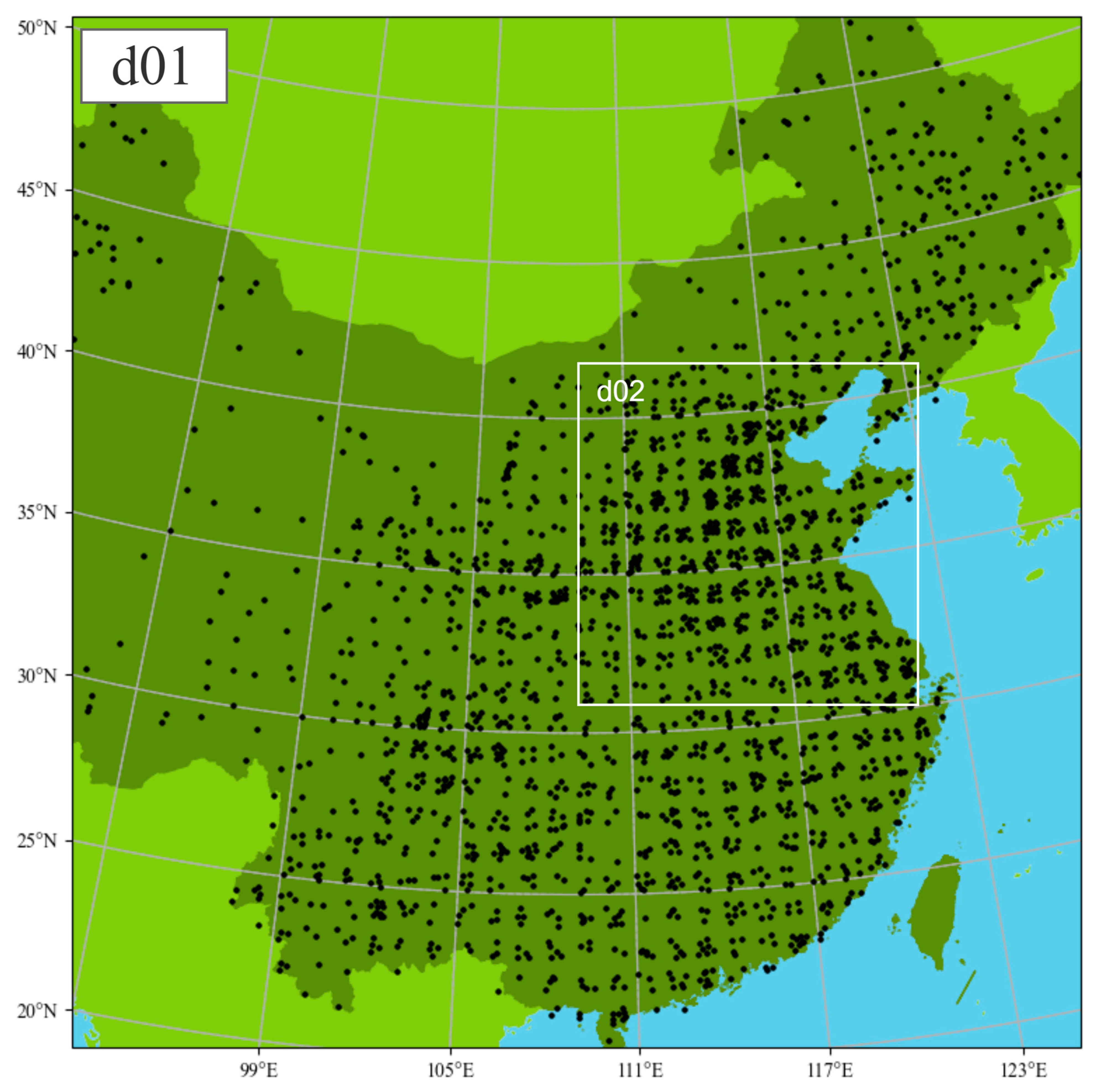
2.1. Model and Data

WRF-Chem v3.9, a new-generation air quality model that couples a chemistry module with the mesoscale weather model WRF, was used to enable the real-time online coupling of meteorology and chemistry.
As illustrated in Figure 1, a two-nested grid approach was employed. The outermost grid (d01) had a horizontal resolution of 27 km, centered at (109.4°E, 36.0°N), with 164 grid cells in the east–west direction and 155 grid cells in the north–south direction, covering most of China. The second inner grid (d02) had a horizontal resolution of 9 km, centered at (114.57°E, 37.98°N), with 175 grid cells in the east–west direction and 166 grid cells in the north–south direction, covering the North China Plain, northeastern China, northern central China, and eastern parts of northwestern China. This study utilized the 2016 Multi-resolution Emission Inventory for China (MEIC) provided by Tsinghua University. The Pollutant Emission Inventory v1.2 covers mainland China and includes emissions of SO2, NOx, CO, NMVOC, NH3, PM2.5, BC, OC, CO2, and other pollutants.
An eta-layer vertical coordinate system with 40 layers in the vertical direction was adopted in the model, with the highest level at 50 hPa. The settings and choices of the physical and chemical parameterization schemes were based on a study by Wang et al. [42]. The Model for Simulating Aerosol Interactions and Chemistry (MOSAIC) scheme was used to simulate the physical and chemical processes of aerosols and has been shown to be more suitable for simulating heavy aerosol pollution episodes in China [43]. To reduce the huge amount of computation caused by numerous aerosol variables, we simplified the variables in the MOSAIC scheme to 20, including the mass concentrations of five species and four particle size segments.
The PM2.5 and PM10 data used in this study were obtained from 1579 ground observation sites between 14 March and 18 March 2021. These data exhibit high accuracy but an inhomogeneous distribution. The quality control method of PM data mainly adopts extreme value control, and therefore the data of PM10 exceeding 9000 µg/m3 and PM2.5 exceeding 5000 µg/m3 were excluded. To enhance the accuracy of the PM data spatiotemporal representation, data points within a grid exceeding the mean by over two standard deviations were excluded from the analysis [4].
The high spatial-temporal resolution AOD data used in the two assimilation experiments were obtained from the Himawari-8 meteorological satellite launched by the Japan Meteorological Agency [44]. These AOD data were at the L3 level with hourly intervals. Prior to use, the data were subjected to stringent cloud screening and quality control procedures to ensure their reliability and accuracy. Additionally, the accuracy of the AOD simulations was verified using Level 1.5 Aerosol Robotic Network (AERONET) aerosol optical thickness products jointly established by the National Aeronautics and Space Administration (NASA) and LOA-PHOTONS (CNRS).

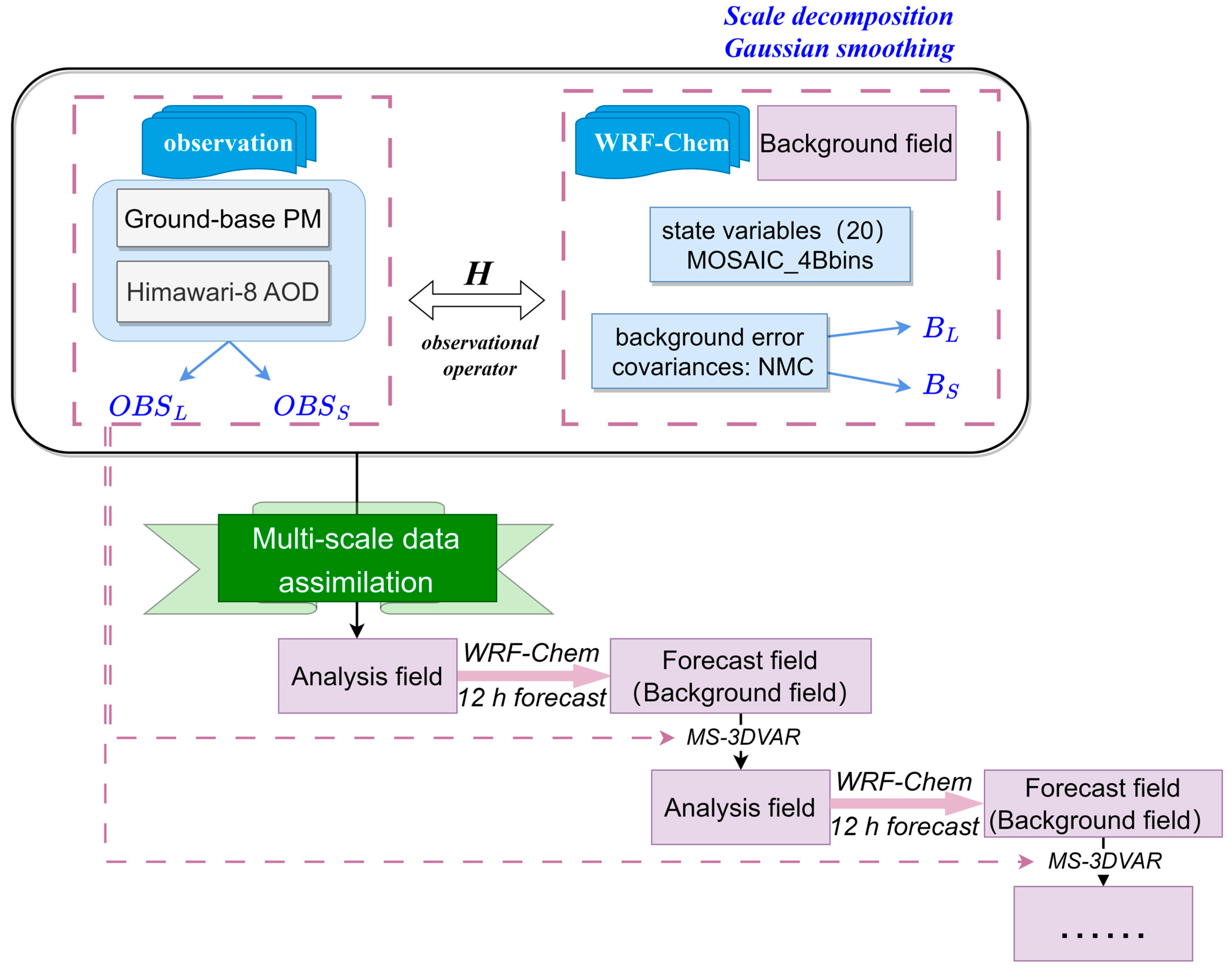
2.2. MS-3DVAR Assimilation

The 3DVAR assimilation method combines the model background field with observational data and uses a descent algorithm to find the minimum solution and then achieves a theoretically optimal analysis [23]. If the background and observational errors conform to a Gaussian distribution, a scalar objective function is formulated based on the principle of least squares. This function quantifies the errors from observations and background errors from models. This formulation transforms the assimilation problem into a mathematical problem to determine the minimum objective function.
The objective function constructed by traditional 3DVAR is as follows:
J ( x ) = 1 2   ( x x b ) T B 1 ( x x b ) + 1 2 ( H X y ) T R 1 H X y
The state estimation vector, denoted as x , is derived from the N-dimensional vector of the state variables on the model grid points. The background field x b represents the background values provided by the model and corresponds to x . The background error covariance matrix B not only characterizes the accuracy of the model simulations but also facilitates the transmission of the observational information to the model grid points. Here, y represents the observational field and R is the observational error covariance. The observation operator H maps the state variables to the observation space, establishing a correspondence between the simulated values from the model variables and the actual observations.
Different observational data contain different scales of information. Background error covariance corresponding to numerical models with different resolutions has different scales of structure and properties. From the perspective of the utilization rate of observation information, the larger the horizontal correlation length (defined as the spatial distance where the correlation decreases from 1 to 1/e), the larger the dissemination range of observation information in the assimilation increment will be. However, the larger the specified horizontal correlation length is, the stronger the filtering of the observation space [26], and the small-scale information obtained from the dense observation network will be filtered out.
To better extract the multi-scale information of the observation field and the background field, the MS-3DVAR method separates the cost function and the assimilation parameter into two scales of size, and the cost function is obtained as follows:
J ( δ x S ) = 1 2   δ x S T B S 1   δ x S + 1 2 ( H δ x S y S ) T R S 1 ( H δ x S y S )
J ( δ x L ) = 1 2   δ x L T B L 1   δ x L + 1 2 ( H δ x L y L ) T R L 1 ( H δ x L y L )
In this study, the scale separation was carried out by Gaussian smoothing. The weight coefficient is expressed as w = e r 2 / 2 D 2 [45], where r is the distance of the observed data to the center of the observed location, and D is the length scale. The smoothed fields after applying the weighted average are taken as the large-scale component, and the residual is taken as the small-scale component. However, in practical applications, using this smoothing treatment, the orthogonality between the large- and small-scale components may be lost, resulting in a decrease in the spatial correlation of the observation errors [15,45,46].
The estimate of B is obtained by using the NMC (National Meteorology Center) method. Each sample is obtained by subtracting the 24 h forecast field from the 48 h forecast field at the same forecast time. For detailed information on the calculation of the B matrix, please refer to Wang et al. [42]. We followed the methodology proposed by Liang et al. [47] to process the observational data. Specifically, we utilized a Gaussian filtering technique to separate the PM and AOD observational data into two distinct components, large-scale y L and small-scale y S , during the assimilation process of MS-3DVAR. This led to the assimilation increment fields δ x L and δ x S for the two scales. The final assimilated analysis field x a was obtained by adding these assimilation increment fields to the background field x b .
To quantitatively assess the improvement induced by the MS-3DVAR assimilation, this study adopted widely used statistical metrics [48], including the correlation coefficient (CORR), root mean squared error (RMSE), and mean fraction error (MFE). The formulae for each metric are as follows:
CORR = i = 1 n O i O ¯ S i S ¯ i = 1 n O i O ¯ 2 i = 1 n S i S ¯ 2
RMSE = 1 n i = 1 n S i O i 2
MFE = 1 n i = 1 n S i O i S i + O i / 2
where n represents the number of valid observation samples and O represents the observed values. Here, S represents the simulated values obtained through interpolation at the observation points, while O ¯ and S ¯ represent the mean of the simulated and observed values, respectively. CORR reflects the correlation between the simulated and observed values, whereas RMSE and MFE quantify the forecast errors of the model. When calculating these metrics for the two sets of assimilation experiments and control experiments, the simulated model values are first interpolated from the grid points to the observation points. Next, we calculate the metric values for various forecast duration, obtaining time series data for each metric. Then, we analyze the impact and duration of the assimilation improvement in the forecast field by comparing the differences in the metric curves among the three sets of experiments.

2.3. Assimilation Scheme Design

This study designed one control experiment (CTL) and two sets of assimilation experiments. The CTL experiment only used models without assimilating the observation data. The MS-3DVAR experiment and the 3DVAR experiment both assimilated PM data and AOD data. These three experiments were conducted from 06:00 UTC on 14 March 2021, to 06:00 UTC on 18 March 2021. Figure 2 illustrates the flowchart of the cycle assimilation process of the MS-3DVAR. The initial background field was generated using the simulation results of a 48 h forecast at 06:00 UTC on 12 March, when various physical quantities of the model reached a dynamic equilibrium state. The background field was assimilated to obtain a more realistic analysis field, which was used as the initial field for the next 12 h forecast. This process was repeated, assimilating the observed data every 12 h (assimilation window). By comparing the PM and AOD observation data with their analysis fields from the two sets of assimilation experiments, the differential improvement effect of the two assimilation methods on the background field can be obtained.

3. Results

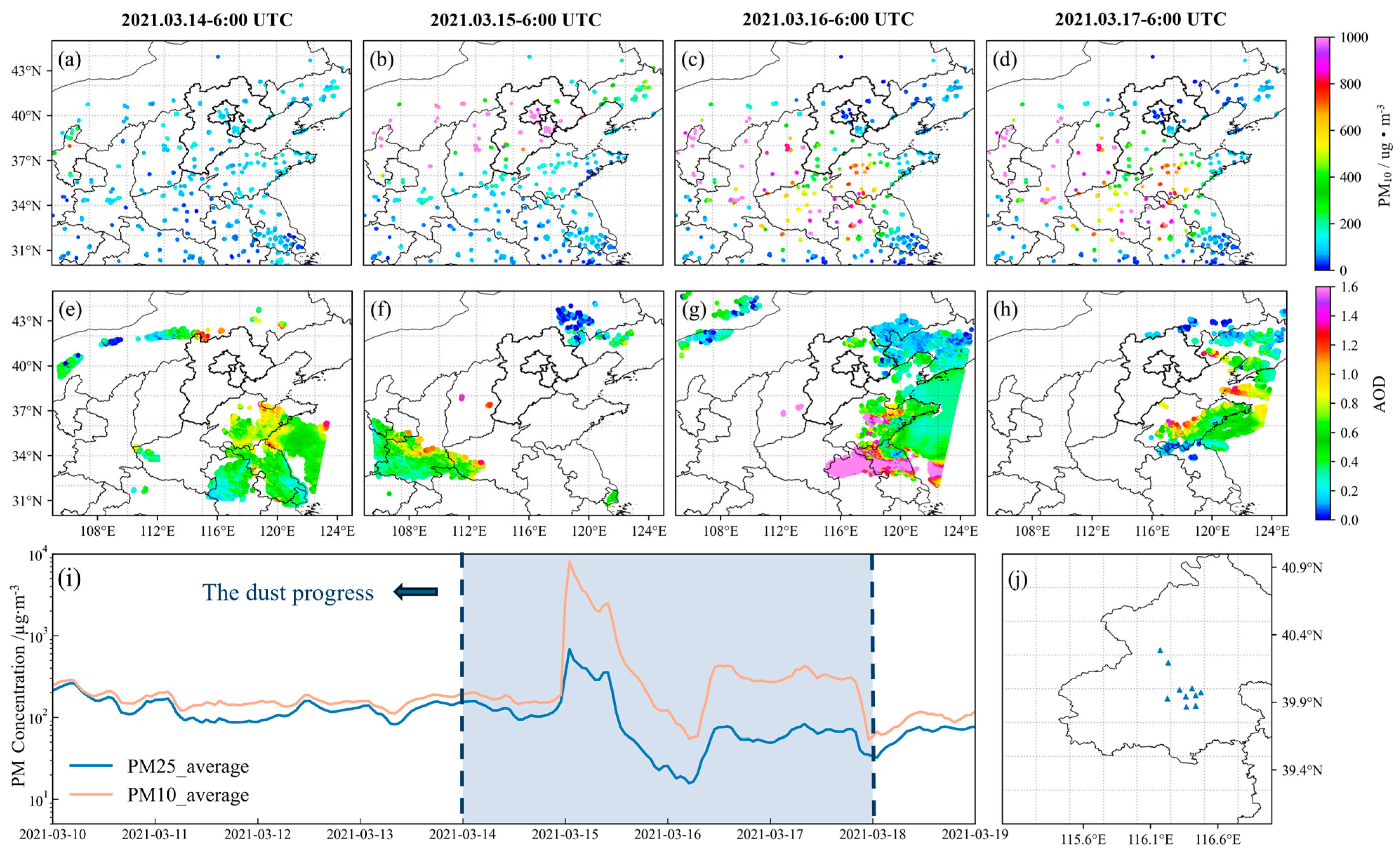
3.1. Observation Analysis

Figure 3 shows that this dust event started roughly on the evening of 14 March, originating from the southeastern part of Inner Mongolia and gradually spreading eastward and southward. By the early morning of 15 March, it had spread to the northern parts of Shanxi, as well as the Beijing–Tianjin–Hebei region, with PM10 concentrations peaking at around 8000 µg/m3. The dust continued to spread southward to northern Henan and the Shandong Peninsula. Dust storms occurred in several regions, including a region between 34°N and 40°N latitude. The dust event in the northwestern regions persisted from March 14 to March 17 and continued to impact southern areas, including Eastern China. During this dust event, the highest hourly PM10 concentration in the Beijing–Tianjin–Hebei region exceeded 5000 µg/m3.
As presented in Figure 3i, the PM data averaged over 10 observation stations in Beijing indicates that the dust event in the Beijing–Tianjin–Hebei region commenced at approximately 00:00 UTC on 15 March and reached its peak within two hours. The PM10 concentrations on the four observation sites in Beijing all exceeded 6000 µg/m3, with the maximum reaching 9000 µg/m3. The dust concentration decreased rapidly in the early morning of 16 March, returning to normal levels. From 12:00 UTC on 16 March onward, the PM concentration began to rapidly increase again and remained at a high level of around 300–400 µg/m3 until 18 March. At around 00:00 UTC on 18 March, the PM10 concentration recovered to around 100 µg/m3, marking the gradual end of this dust event.
Figure 3e shows that the high AOD on March 14 was mainly concentrated in eastern Jiangsu, and from 14 to 17 March, the high pollution value area moved eastward and southward, continuously expanding its range. As shown in Figure 3f, valid retrievals of AOD from the Himawari-8 satellite were only possible in the southern part of Shaanxi and the western part of Henan owing to the cloud coverage in the remanent regions over eastern and northern China on 15 March. Figure 3g shows the widespread aerosol pollution event in eastern China on 16 March, including Shandong province and the northern part of Jiangsu province. However, the distribution and quantity of observational data had a significant impact on the assimilation outcomes. The majority of AOD retrievals from Himawari-8 in the Beijing–Tianjin–Hebei region are missing during 14–17 March, which might have affected the simulation of the assimilated AOD data.

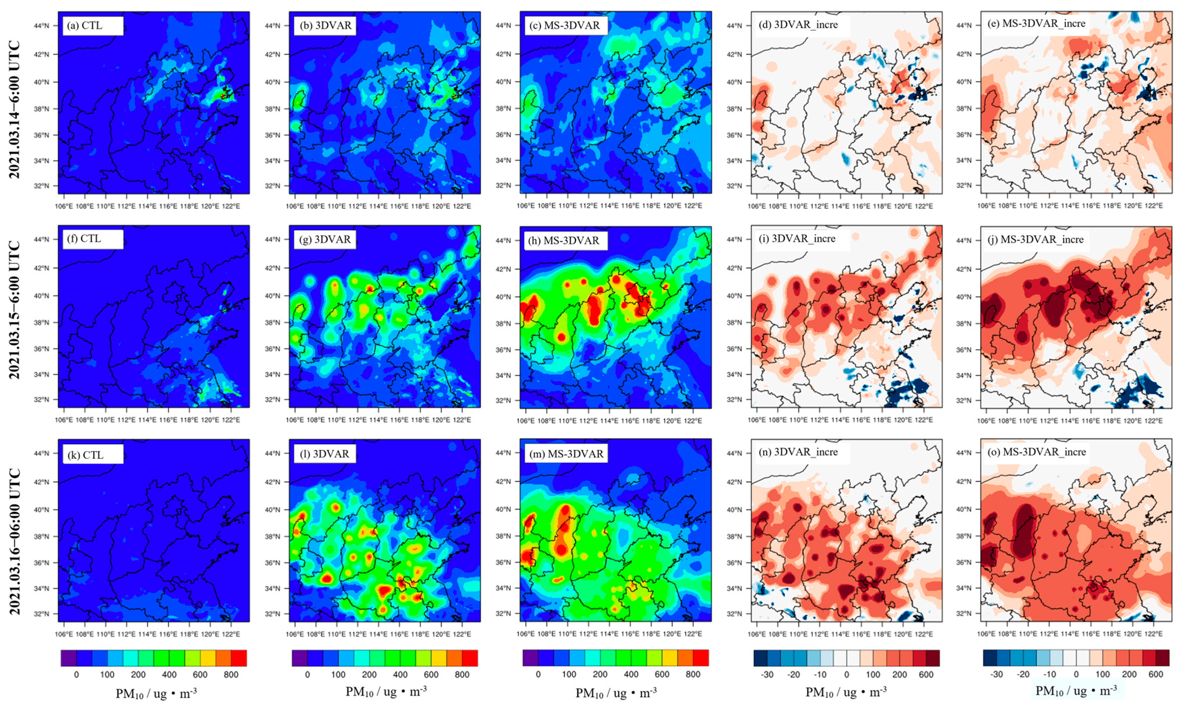
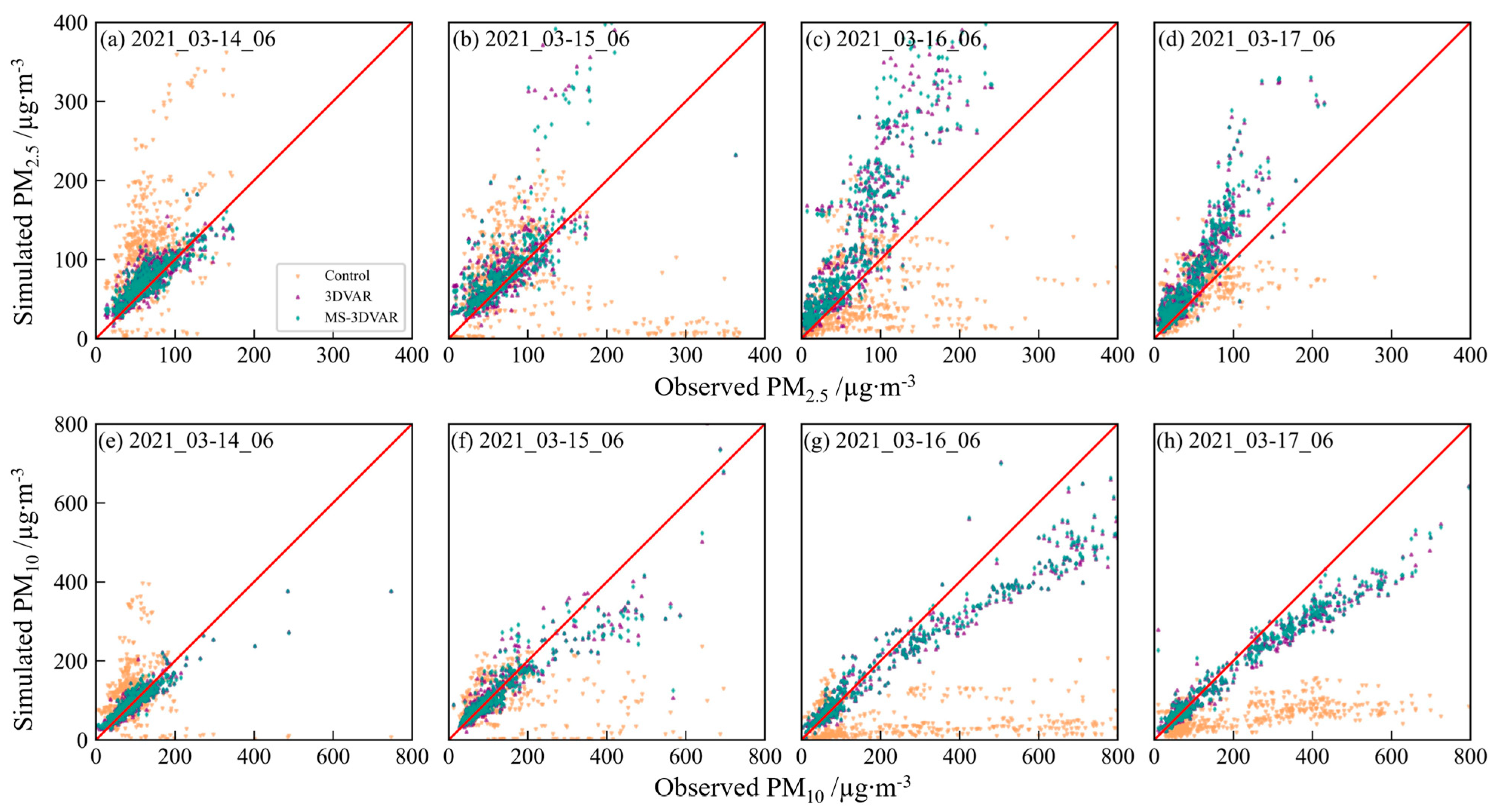
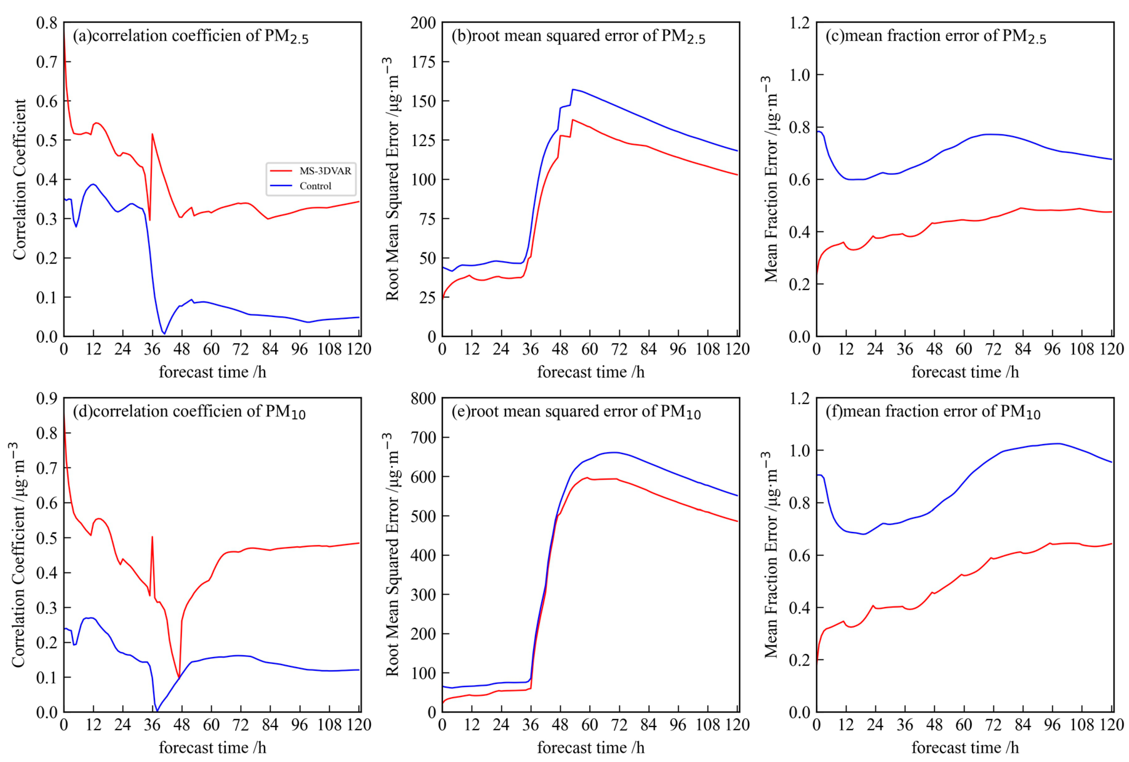
3.2. PM Assimilation Effect Analysis

The assimilations form incremental fields based on the background field, and then we use their sum (analysis field) to forecast weather in the model, to improve the forecasting accuracy. Figure 4 presents the surface distribution of the PM10 increment field from 14 to 16 March. The first column illustrates the background field of the control experiment. The second and third column present the PM10 mass concentration in the analysis field, which was obtained through 3DVAR and MS-3DVAR assimilation experiments by jointly assimilating the PM and AOD data. The last two columns show the PM10 increment field, which represents the difference between the assimilation and control experiments.
The first column of Figure 4 shows that the model simulations generally underestimated the pollutant concentrations and extent in most of the simulation area. The distribution of the increment fields (the last two columns) indicates a prominent high-value area at the intersection of Inner Mongolia, Shaanxi, and Shanxi, which is closer to the observed values. Owing to the overlapping increments from nearby observation stations, the increment fields do not exhibit a circular distribution centered around the observation points. Additionally, the assimilated increments dynamically move downstream with the wind flow, leading to an expanded distribution range.
Compared with the increment fields obtained from the 3DVAR assimilation experiments, the MS-3DVAR assimilation yielded larger and better-fitting extreme values of pollutant concentrations in the analytical fields. In addition, the diffusion of pollutants to the surrounding area was larger, indicating that the MS-3DVAR assimilation method effectively utilized the multi-scale information of the observed data to generate a more accurate analysis field. Despite the obvious improvement in aerosol concentration simulation accuracy through data assimilation, a discrepancy still exists between the assimilated analysis field and the extreme PM10 values observed.
Figure 5 presents a statistical analysis of the results of the control experiment and two sets of assimilation experiments on 06 UTC, 14 to 17 March 2021 within the d02 domain. The red centerline indicates the consistency degree between the model and observed values with missing values excluded. The orange dots of the control experiments exhibit a significant dispersion on both sides of the centerline, indicating that the simulated values of the background field are inaccurate. The upper and lower lines show the scatter distribution of PM10 and PM2.5, respectively, with the purple and green dots, respectively, representing the results of the 3DVAR and the MS-3DVAR assimilation experiments.
The models exhibit a tendency to overestimate the PM2.5 and underestimate the PM10 concentrations. As the dust event develops, the control experiment shows an increasing underestimation between the model-simulated values and observed data. The dispersion of MS-3DVAR is more concentrated, indicating that the assimilation effect is better than that of 3DVAR.
After data assimilation, the tightly distributed green dots on both sides of the red centerline indicate that the simulated analysis fields show an improved consistency with the actual observations, especially for PM2.5 and PM10 observations exceeding 150 µg/m3. That contributes to the background field effectively incorporating the aerosol observation information, resulting in an optimal analysis field closely aligned with the red centerline.
Table 1 shows the statistical metrics, indicating the four initial times of each assimilation window. The CORR between the MS-3DVAR assimilated PM10 simulated values and observations increases from 0.24 to 0.93. The RMSE decreases from 85.08 µg/m3 to 25.30 µg/m3 at 6:00UTC March 14, a reduction of 59.79 µg/m3 (70.3%). In all cases, data assimilation increases the CORR between the model simulation and observations to above 0.8 while reducing the RMSE by approximately 40%. Both statistical metrics consistently indicate that the MS-3DVAR assimilation has a significant impact on enhancing the background field, with the metrics of MS-3DVAR outperforming those of 3DVAR.

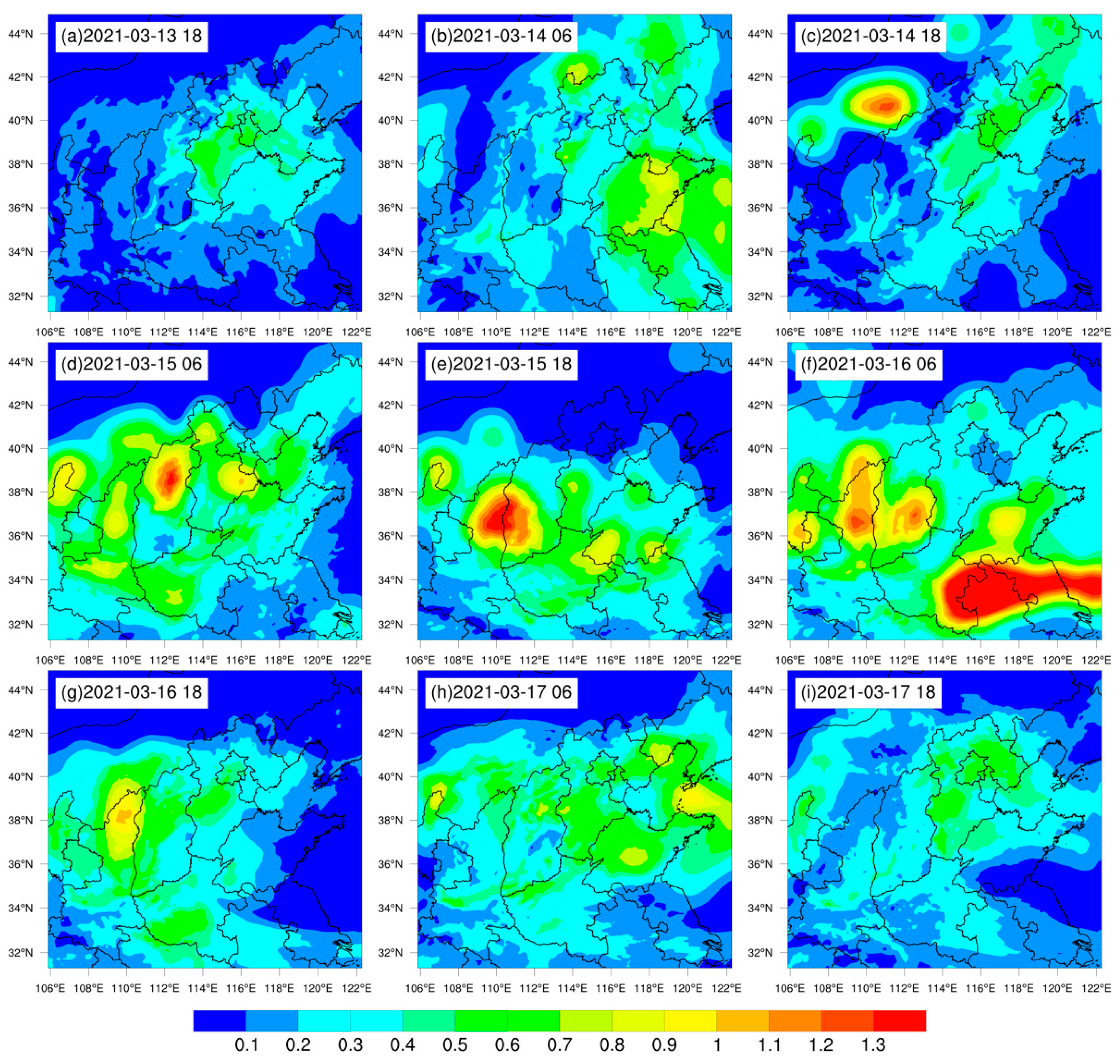
3.3. AOD Assimilation Effect Analysis

Figure 6 shows the AOD distribution of the MS-3DVAR assimilation experiment from 13 to 17 March 2021. Interestingly, the area with the maximum simulated AOD was found to spread over the eastern part of Henan province and the northern part of Anhui province on March 16 at 06:00 UTC. This pattern closely matches the observations in Figure 3, indicating that assimilation has a clear improvement effect on the simulated AOD.
The model shows a tendency to underestimate the AOD data. Compared to the orange dots, the green dots in Figure 7 indicate that the AOD simulation fits more closely to the red central lines, suggesting a significant improvement in the AOD simulation after MS-3DVAR assimilation was performed. This improvement was more pronounced for values of AOD < 1, and the simulations for AOD > 1 still fall short of the observations. As previously mentioned, assimilation significantly improved the background fields of the model, which determine the accuracy of the forecast fields. However, owing to the accumulation of model errors, emission source uncertainties, and other uncertain factors, the improvement effect of assimilation on the forecast results diminished as the forecast time progressed.
Figure 8 shows the statistical metrics curves between the simulated values of PM2.5 (upper row), PM10 (lower row) and the observations in the CTL experiment (blue line) and MS-3DVAR assimilation (red line) experiment of the forecast time. At the beginning of the forecast, the CORRs of the MS-3DVAR assimilation experiment for PM2.5 and PM10 both exceeded 0.7, while in the CTL experiment, the CORRs for PM2.5 and PM10 were 0.35 and 0.25, respectively, with the greatest disparity between them. Over the first 12 h of forecasting, the CORR in the MS-3DVAR assimilation experiment rapidly decreased, whereas in the CTL experiment, it experienced a slight improvement during the model’s dynamic adjustment process, with an average difference of 0.2. Within the first 24 h of the forecast, the difference in the statistical metrics between the MS-3DVAR assimilation and the CTL experiments gradually decreased. It is worth noting that around the 40th hour of the forecast, there was a peak in the CORR of the MS-3DVAR assimilation experiment, which corresponds to the minimum value in the CORR of the CTL experiment. This may be due to an abnormally high peak of PM at 01:00 UTC on 15 March, and the WRF-Chem model significantly underestimated the pollution process at that time.
Furthermore, regarding the RMSE, the positive impact of MS-3DVAR assimilation was particularly pronounced within the initial 36 h of the forecast. Subsequently, there was a notable surge between the 36th and 60th hours, succeeded by a gradual decline. The RMSE for PM10 notably exceeded that for PM2.5, with a larger disparity between the CTL and MS-3DVAR assimilation experiments for PM10, signifying lower model accuracy in simulating PM10 but a more substantial improvement effect through MS-3DVAR assimilation. Specifically, assimilation leads to a reduction in the average relative error of PM2.5 by 0.3 µg/m3 and PM10 by 0.4 µg/m3. As assimilation occurs every 12 h, the average MFE exhibits fluctuations within this 12 h interval. These fluctuations demonstrate a diminishing trend with increasing forecast time, suggesting a reduction in assimilation effectiveness over time.
Upon comparing various statistical metrics, it is noted that MS-3DVAR assimilation contributed to improvements in the forecast field within the initial 36 h of the forecast. However, with the progression of forecast time, the assimilation effect may exhibit a slight reduction due to the influence of external forcing factors, such as emission sources. In summary, assimilation consistently enhances the simulated outcomes.
Figure 9 shows the comparison of AOD (black dots) measured at the Beijing_CAMS (39.93°N, 116.32°E) site in the Beijing–Tianjin–Hebei region from 14 to 18 March 2021. The simulated AOD was obtained from the CTL (red line) and MS-3DVAR assimilation (black line) experiments. The yellow represents the PM10 and the green represents the PM2.5 simulated by the MS-3DVAR. The simulated AOD was significantly elevated in the early morning of March 15. This indicates a significant enhancement in the AOD simulation, attributed to the assimilation of the observed peak PM data into the model. The PM value simulated by MS-3DVAR is in good agreement with the AOD value.
At around 00:00 on 16 March, the pollution level in Beijing was relatively low, and the measured AOD data were as low as about 0.2–0.3. Since the early morning of 16 March, the AOD value of the MS-3DVAR assimilation test was continuously higher than that of the CTL test, and the consistency with the measured value of AERONET was also improved. Overall, MS-3DVAR assimilation can improve the simulation of AOD. Since the initial field cycle is updated every 12 h in the forecast, the improvement effect of the assimilation test shows a fluctuating trend.

4. Conclusions

This study aimed to investigate the effectiveness of the MS-3DVAR approach in improving the prediction accuracy of a record-breaking sandstorm event in the Beijing–Tianjin–Hebei region from 14 to 18 March 2021. To achieve this goal, a cycling assimilation experiment that integrated ground-level PM2.5, PM10, and Himawari-8 satellite AOD data using the MS-3DVAR method and the WRF-Chem model was conducted in this study. The performance of the MS-3DVAR technique was evaluated by conducting a comprehensive assessment, which included a comparison with a control experiment conducted without assimilated data and the traditional 3DVAR method.
Based on observational data, the d02 region identified Beijing and Tianjin as heavily polluted areas on 15 March 2021, with PM10 concentrations exceeding 5000 µg/m3. In contrast, the control experiment simulation underestimated the concentrations, with levels below 1000 µg/m3. When using a single horizontal length-scale parameter to construct the background error covariance with the traditional assimilation method, the complete information of the high-resolution observational data could not be fully utilized, and small-scale observational information tended to be filtered out. By adopting multiple scales of the background error covariance, the large-scale horizontal correlation parameters enabled the observational information to propagate more widely in assimilation increments. In contrast, the small-scale horizontal correlation parameters allowed the filtered observational information in the large-scale processes to be more fully utilized.
Specifically, the MS-3DVAR assimilation of multiple aerosol data sources significantly improved the accuracy of the model simulation, resulting in more precise initial fields. The CORR between the assimilated PM10 initial fields and observations increased from 0.24 to 0.93. RMSE decreased from 85.08 µg/m3 to 25.30 µg/m3 with a reduction up to 59.79 µg/m3 (70.3%). These consistent improvements in both the CORR and RMSE indicate a significant enhancement of assimilation in the initial fields of the pollutants.
Assimilating the aerosol data also improved both the PM and AOD forecasts, with a greater impact on PM10 than PM2.5. The CORR, RMSE, and MFE statistics showed consistent improvements in the PM and AOD forecasts within the 36 h assimilation period. The curves of the three statistical metrics demonstrated maximum differences at the initial time of forecast, followed by reduced fluctuations, indicating a diminishing improvement effect over time.
During the initial time on 14 March, at 06:00, the coverage of the satellite AOD data was limited, leading to inadequate data availability for assimilation. Therefore, the assimilation exhibited relatively limited improvement, highlighting the urgent need to address the challenges associated with the quality control, correction, and high-precision inversion of the satellite AOD data during heavy dust events. Although the MS-3DVAR assimilation improved the simulation effect of pollutants to a certain extent, there was still a gap between the simulated results and the actual observations. In the future, we not only hope to optimize the background error covariance in a multi-scale way, but also hope to use more observational data in the assimilation system to improve the accuracy of model prediction.

Author Contributions

Conceptualization, W.Y. and W.Z.; methodology, S.M.; validation, W.Z., W.Y. and J.G.; formal analysis, S.M.; investigation, Q.X.; resources, W.Z., W.Y. and Z.Z.; data curation, S.M.; writing—original draft preparation, S.M.; writing—review and editing, W.Z., W.Y. and J.G.; visualization, S.M.; supervision, W.Z. and W.Y. All authors have read and agreed to the published version of the manuscript.

Funding

This research was funded by the Natural Science Foundation of Hunan Province-Outstanding Youth Foundation, grant number No. 2023JJ20050 and the National Natural Science Foundation of China under grants U2142209 and 42075011.

Data Availability Statement

The ground particulate matter concentration data used to support the conclusions in this study can be downloaded at the China National Environmental Monitoring Center via https://air.cnemc.cn:18007/, accessed on 21 May 2023. The research product of aerosol properties (produced from Himawari-8) can be downloaded at https://www.eorc.jaxa.jp/ptree/userguide.html, accessed on 21 May 2023. The used Level 1.5 Aerosol Robotic Network (AERONET) aerosol optical thickness products jointly established by the National Aeronautics and Space Administration (NASA) and LOA-PHOTONS (CNRS) is available at https://aeronet.gsfc.nasa.gov/, accessed on 21 May 2023.

Conflicts of Interest

The authors declare no conflicts of interest.

References

  1. Gui, K.; Yao, W.; Che, H.; An, L.; Zheng, Y.; Li, L.; Zhao, H.; Zhang, L.; Zhong, J.; Wang, Y.; et al. Record-Breaking Dust Loading during Two Mega Dust Storm Events over Northern China in March 2021: Aerosol Optical and Radiative Properties and Meteorological Drivers. Atmos. Chem. Phys. 2022, 22, 7905–7932. [Google Scholar] [CrossRef]
  2. Filonchyk, M.; Peterson, M. Development, Progression, and Impact on Urban Air Quality of the Dust Storm in Asia in March 15–18, 2021. Urban Clim. 2022, 41, 101080. [Google Scholar] [CrossRef]
  3. Jin, J.; Pang, M.; Segers, A.; Han, W.; Fang, L.; Li, B.; Feng, H.; Lin, H.X.; Liao, H. Inverse Modeling of the 2021 Spring Super Dust Storms in East Asia. Atmos. Chem. Phys. 2022, 22, 6393–6410. [Google Scholar] [CrossRef]
  4. Zeng, Y.; Wang, M.; Zhao, C.; Chen, S.; Liu, Z.; Huang, X.; Gao, Y. WRF-Chem v3.9 Simulations of the East Asian Dust Storm in May 2017: Modeling Sensitivities to Dust Emission and Dry Deposition Schemes. Geosci. Model Dev. 2020, 13, 2125–2147. [Google Scholar] [CrossRef]
  5. Nazzal, Y.; Barbulescu, A.; Howari, F.; Yousef, A.; Al-Taani, A.A.; Al Aydaroos, F.; Naseem, M. New Insights on Sand Dust Storm from Historical Records, UAE. Arab. J. Geosci. 2019, 12, 396. [Google Scholar] [CrossRef]
  6. Gui, K.; Yao, W.; Che, H.; An, L.; Zheng, Y.; Li, L.; Zhao, H.; Zhang, L.; Zhong, J.; Wang, Y.; et al. Two Mega Sand and Dust Storm Events over Northern China in March 2021: Transport Processes, Historical Ranking and Meteorological Drivers. Atmos. Chem. Phys. Discuss. 2021, 1, 36. [Google Scholar]
  7. Ye, Q.; Zheng, X. Distribution, Transport, and Impact on Air Quality of Two Typical Dust Events in China in 2021. Atmosphere 2023, 14, 432. [Google Scholar] [CrossRef]
  8. Liang, P.; Chen, B.; Yang, X.; Liu, Q.; Li, A.; Mackenzie, L.; Zhang, D. Revealing the Dust Transport Processes of the 2021 Mega Dust Storm Event in Northern China. Sci. Bull. 2022, 67, 21–24. [Google Scholar] [CrossRef] [PubMed]
  9. Yasunari, T.J.; Koster, R.D.; Lau, W.K.M.; Kim, K. Impact of Snow Darkening via Dust, Black Carbon, and Organic Carbon on Boreal Spring Climate in the Earth System. J. Geophys. Res. Atmos. 2015, 120, 5485–5503. [Google Scholar] [CrossRef]
  10. Escribano, J.; Di Tomaso, E.; Jorba, O.; Klose, M.; Gonçalves Ageitos, M.; Macchia, F.; Amiridis, V.; Baars, H.; Marinou, E.; Proestakis, E.; et al. Assimilating Spaceborne Lidar Dust Extinction Improves Dust Forecasts. Atmos. Chem. Phys. Discuss. 2022, 22, 535–560. [Google Scholar] [CrossRef]
  11. Sokhi, R.S.; Moussiopoulos, N.; Baklanov, A.; Bartzis, J.; Coll, I.; Finardi, S.; Friedrich, R.; Geels, C.; Grönholm, T.; Halenka, T.; et al. Advances in Air Quality Research—Current and Emerging Challenges. Atmos. Chem. Phys. 2022, 22, 4615–4703. [Google Scholar] [CrossRef]
  12. Carmichael, G.R.; Sandu, A.; Chai, T.; Daescu, D.N.; Constantinescu, E.M.; Tang, Y. Predicting Air Quality: Improvements through Advanced Methods to Integrate Models and Measurements. J. Comput. Phys. 2008, 227, 3540–3571. [Google Scholar] [CrossRef]
  13. Wang, J.; Zhang, B.; Zhang, H.; Hua, C.; An, L.; Gui, H. Simulation of a Severe Sand and Dust Storm Event in March 2021 in Northern China: Dust Emission Schemes Comparison and the Role of Gusty Wind. Atmosphere 2022, 13, 108. [Google Scholar] [CrossRef]
  14. Cheng, X.; Liu, Y.; Xu, X.; You, W.; Zang, Z.; Gao, L.; Chen, Y.; Su, D.; Yan, P. Lidar Data Assimilation Method Based on CRTM and WRF-Chem Models and Its Application in PM2.5 Forecasts in Beijing. Sci. Total Environ. 2019, 682, 541–552. [Google Scholar] [CrossRef] [PubMed]
  15. Li, Z.; Cheng, X.; Gustafson, W.I., Jr.; Vogelmann, A.M. Spectral Characteristics of Background Error Covariance and Multiscale Data Assimilation. Int. J. Numer. Methods Fluids 2016, 82, 1035–1048. [Google Scholar] [CrossRef]
  16. Wang, Y.; Sartelet, K.N.; Bocquet, M.; Chazette, P. Assimilation of Ground versus Lidar Observations for PM10 Forecasting. Atmos. Chem. Phys. 2013, 13, 269–283. [Google Scholar] [CrossRef]
  17. Luo, H.; Dong, L.; Chen, Y.; Zhao, Y.; Zhao, D.; Huang, M.; Ding, D.; Liao, J.; Ma, T.; Hu, M.; et al. Interaction between Aerosol and Thermodynamic Stability within the Planetary Boundary Layer during Wintertime over the North China Plain: Aircraft Observation and WRF-Chem Simulation. Atmos. Chem. Phys. 2022, 22, 2507–2524. [Google Scholar] [CrossRef]
  18. Ha, S.; Kumar, R.; Pfister, G.G.; Lee, Y.; Lee, D.; Kim, H.M.; Ryu, Y.-H. Chemical Data Assimilation with Aqueous Chemistry in WRF-Chem Coupled with WRFDA (V4.4.1). J. Adv. Model. Earth Syst. 2023, 16, e2023MS003928. [Google Scholar] [CrossRef]
  19. Eltahan, M.; Shokr, M.; Sherif, A. Simulation of Severe Dust Events over Egypt Using Tuned Dust Schemes in Weather Research Forecast (WRF-Chem). Atmosphere 2018, 9, 246. [Google Scholar] [CrossRef]
  20. Benedetti, A.; Morcrette, J.-J.; Boucher, O.; Dethof, A.; Engelen, R.J.; Fisher, M.; Flentje, H.; Huneeus, N.; Jones, L.; Kaiser, J.W.; et al. Aerosol Analysis and Forecast in the European Centre for Medium-Range Weather Forecasts Integrated Forecast System: 2. Data Assimilation. J. Geophys. Res. Atmos. 2009, 114, 2008JD011115. [Google Scholar] [CrossRef]
  21. Li, Z.; Zang, Z.; Li, Q.B.; Chao, Y.; Chen, D.; Ye, Z.; Liu, Y.; Liou, K.N. A Three-Dimensional Variational Data Assimilation System for Multiple Aerosol Species with WRF/Chem and an Application to PM2.5 Prediction. Atmos. Chem. Phys. 2013, 13, 4265–4278. [Google Scholar] [CrossRef]
  22. Vendrasco, E.P.; Sun, J.; Herdies, D.L.; Frederico De Angelis, C. Constraining a 3DVAR Radar Data Assimilation System with Large-Scale Analysis to Improve Short-Range Precipitation Forecasts. J. Appl. Meteorol. Climatol. 2016, 55, 673–690. [Google Scholar] [CrossRef]
  23. Zang, Z.; You, W.; Ye, H.; Liang, Y.; Li, Y.; Wang, D.; Hu, Y.; Yan, P. 3DVAR Aerosol Data Assimilation and Evaluation Using Surface PM2.5, Himawari-8 AOD and CALIPSO Profile Observations in the North China. Remote Sens. 2022, 14, 4009. [Google Scholar] [CrossRef]
  24. Bocquet, M.; Elbern, H.; Eskes, H.; Hirtl, M.; Žabkar, R.; Carmichael, G.R.; Flemming, J.; Inness, A.; Pagowski, M.; Pérez Camaño, J.L.; et al. Data Assimilation in Atmospheric Chemistry Models: Current Status and Future Prospects for Coupled Chemistry Meteorology Models. Atmos. Chem. Phys. 2015, 15, 5325–5358. [Google Scholar] [CrossRef]
  25. Pu, Z.; Kalnay, E. Numerical Weather Prediction Basics: Models, Numerical Methods, and Data Assimilation. In Handbook of Hydrometeorological Ensemble Forecasting; Duan, Q., Pappenberger, F., Thielen, J., Wood, A., Cloke, H.L., Schaake, J.C., Eds.; Springer: Berlin/Heidelberg, Germany, 2018; pp. 1–31. ISBN 978-3-642-40457-3. [Google Scholar]
  26. Zang, Z.; Liang, Y.; You, W.; Li, Y.; Pan, X.; Li, Z. Multi-Scale Three-Dimensional Variational Data Assimilation for High-Resolution Aerosol Observations: Methodology and Application. Sci. China Earth Sci. 2022, 65, 1961–1971. [Google Scholar] [CrossRef]
  27. Xie, X.; Myhre, G.; Shindell, D.; Faluvegi, G.; Takemura, T.; Voulgarakis, A.; Shi, Z.; Li, X.; Xie, X.; Liu, H.; et al. Anthropogenic Sulfate Aerosol Pollution in South and East Asia Induces Increased Summer Precipitation over Arid Central Asia. Commun. Earth Environ. 2022, 3, 328. [Google Scholar] [CrossRef]
  28. Li, J.; Geer, A.J.; Okamoto, K.; Otkin, J.A.; Liu, Z.; Han, W.; Wang, P. Satellite All-Sky Infrared Radiance Assimilation: Recent Progress and Future Perspectives. Adv. Atmos. Sci. 2022, 39, 9–21. [Google Scholar] [CrossRef]
  29. Yang, T.; Li, H.; Wang, H.; Sun, Y.; Chen, X.; Wang, F.; Xu, L.; Wang, Z. Vertical Aerosol Data Assimilation Technology and Application Based on Satellite and Ground Lidar: A Review and Outlook. J. Environ. Sci. 2023, 123, 292–305. [Google Scholar] [CrossRef]
  30. Kim, M.; Lee, K.; Lee, Y.H. Visibility Data Assimilation and Prediction Using an Observation Network in South Korea. Pure Appl. Geophys. 2020, 177, 1125–1141. [Google Scholar] [CrossRef]
  31. Rubin, J.I.; Reid, J.S.; Hansen, J.A.; Anderson, J.L.; Holben, B.N.; Xian, P.; Westphal, D.L.; Zhang, J. Assimilation of AERONET and MODIS AOT Observations Using Variational and Ensemble Data Assimilation Methods and Its Impact on Aerosol Forecasting Skill. J. Geophys. Res. Atmos. 2017, 122, 4967–4992. [Google Scholar] [CrossRef]
  32. Huang, X.; Ding, A. Aerosol as a Critical Factor Causing Forecast Biases of Air Temperature in Global Numerical Weather Prediction Models. Sci. Bull. 2021, 66, 1917–1924. [Google Scholar] [CrossRef] [PubMed]
  33. Liu, R.; Lu, Q.; Wu, C.; Ni, Z.; Wang, F. Assimilation of Hyperspectral Infrared Atmospheric Sounder Data of FengYun-3E Satellite and Assessment of Its Impact on Analyses and Forecasts. Remote Sens. 2024, 16, 908. [Google Scholar] [CrossRef]
  34. Gumber, A.; Reid, J.S.; Holz, R.E.; Eck, T.F.; Hsu, N.C.; Levy, R.C.; Zhang, J.; Veglio, P. Assessment of Severe Aerosol Events from NASA MODIS and VIIRS Aerosol Products for Data Assimilation and Climate Continuity. Atmos. Meas. Tech. 2023, 16, 2547–2573. [Google Scholar] [CrossRef]
  35. Quan, J.; Tie, X.; Zhang, Q.; Liu, Q.; Li, X.; Gao, Y.; Zhao, D. Characteristics of Heavy Aerosol Pollution during the 2012–2013 Winter in Beijing, China. Atmos. Environ. 2014, 88, 83–89. [Google Scholar] [CrossRef]
  36. Tsay, S.-C.; Maring, H.B.; Lin, N.-H.; Buntoung, S.; Chantara, S.; Chuang, H.-C.; Gabriel, P.M.; Goodloe, C.S.; Holben, B.N.; Hsiao, T.-C.; et al. Satellite-Surface Perspectives of Air Quality and Aerosol-Cloud Effects on the Environment: An Overview of 7-SEAS/BASELInE. Aerosol Air Qual. Res. 2016, 16, 2581–2602. [Google Scholar] [CrossRef]
  37. Gao, Z.; Zhou, X. A Review of the CAMx, CMAQ, WRF-Chem and NAQPMS Models: Application, Evaluation and Uncertainty Factors. Environ. Pollut. 2024, 343, 123183. [Google Scholar] [CrossRef]
  38. Saide, P.E.; Carmichael, G.R.; Liu, Z.; Schwartz, C.S.; Lin, H.C.; Da Silva, A.M.; Hyer, E. Aerosol Optical Depth Assimilation for a Size-Resolved Sectional Model: Impacts of Observationally Constrained, Multi-Wavelength and Fine Mode Retrievals on Regional Scale Analyses and Forecasts. Atmos. Chem. Phys. 2013, 13, 10425–10444. [Google Scholar] [CrossRef]
  39. Majumdar, S.J.; Sun, J.; Golding, B.; Joe, P.; Dudhia, J.; Caumont, O.; Chandra Gouda, K.; Steinle, P.; Vincendon, B.; Wang, J.; et al. Multiscale Forecasting of High-Impact Weather: Current Status and Future Challenges. Bull. Am. Meteorol. Soc. 2021, 102, E635–E659. [Google Scholar] [CrossRef]
  40. Ding, Y.; Liang, P.; Liu, Y.; Zhang, Y. Multiscale Variability of Meiyu and Its Prediction: A New Review. J. Geophys. Res. Atmos. 2020, 125, e2019JD031496. [Google Scholar] [CrossRef]
  41. Gustafsson, N.; Janjić, T.; Schraff, C.; Leuenberger, D.; Weissmann, M.; Reich, H.; Brousseau, P.; Montmerle, T.; Wattrelot, E.; Bučánek, A.; et al. Survey of Data Assimilation Methods for Convective-scale Numerical Weather Prediction at Operational Centres. Q. J. R. Meteorol. Soc. 2018, 144, 1218–1256. [Google Scholar] [CrossRef]
  42. Wang, D.; You, W.; Zang, Z.; Pan, X.; Hu, Y.; Liang, Y. A Three-Dimensional Variational Data Assimilation System for Aerosol Optical Properties Based on WRF-Chem: Design, Development, and Application of Assimilating Himawari-8 Aerosol Observations. Geosci. Model Dev. 2021, 15, 1821–1840. [Google Scholar] [CrossRef]
  43. Chen, D.; Liu, Z.; Fast, J.; Ban, J. Simulations of Sulfate-Nitrate-Ammonium (SNA) Aerosols during the extreme haze events over Northern China in October 2014. Atmos. Chem. Phys. 2016, 16, 10707–10724. [Google Scholar] [CrossRef]
  44. Wang, S.; Dai, T.; Li, C.; Cheng, Y.; Huang, G.; Shi, G. Improving Clear-Sky Solar Power Prediction over China by Assimilating Himawari-8 Aerosol Optical Depth with WRF-Chem-Solar. Remote Sens. 2022, 14, 4990. [Google Scholar] [CrossRef]
  45. Li, Z.; McWilliams, J.C.; Ide, K.; Farrara, J.D. A Multiscale Variational Data Assimilation Scheme: Formulation and Illustration. Mon. Weather Rev. 2015, 143, 3804–3822. [Google Scholar] [CrossRef]
  46. Pang, J. The Impacts of Background Error Covariance on Particulate Matter Assimilation and Forecast: An Ideal Case Study with a Modal Aerosol Model over China. Sci. Total Environ. 2021, 786, 147417. [Google Scholar] [CrossRef]
  47. Liang, Y.; Zang, Z.; Liu, D.; Yan, P.; Hu, Y.; Zhou, Y.; You, W. Development of a Three-Dimensional Variational Assimilation System for Lidar Profile Data Based on a Size-Resolved Aerosol Model in WRF–Chem Model v3.9.1 and Its Application in PM2.5 Forecasts across China. Geosci. Model Dev. 2020, 13, 6285–6301. [Google Scholar] [CrossRef]
  48. Boylan, J.W.; Russell, A.G. PM and Light Extinction Model Performance Metrics, Goals, and Criteria for Three-Dimensional Air Quality Models. Atmos. Environ. 2006, 40, 4946–4959. [Google Scholar] [CrossRef]
Figure 1. The simulation domain d01 (black box) and d02 (white box) superimposed with surface meteorological observation sites (black dots).
Remotesensing 16 01852 g001
Figure 2. The flowchart of the cycle assimilation of MS-3DVAR (the symbolism of the last box means that the above process is repeated to achieve cyclic assimilation).
Remotesensing 16 01852 g002
Figure 3. PM10 concentrations (μg/m3) at ground-based atmospheric environmental monitoring stations (ad,i) and the Himawari-8 aerosol optical depth (AOD, eh) in the simulation area d02 for 14–17 March 2021. Also shown are the time series of hourly PM10 (yellow curve) and PM2.5 (blue curve) concentrations averaged over 10 ground-based environmental monitoring stations (j) in Beijing.
Remotesensing 16 01852 g003
Figure 4. Horizontal distribution of PM10 (µg/m3) as simulated by CTL (the first column), 3DVAR (the second column) and MS-3DVAR (the third column) as well as their corresponding incremental fields (the last two columns) at 06 UTC on 14–16 March 2023.
Remotesensing 16 01852 g004
Figure 5. Scattered distribution of PM2.5 (µg/m3, upper row) and PM10 (µg/m3, lower row) in the simulated initial time of the CTL experiment (orange dots), MS-3DVAR experiment (green dots), and 3DVAR experiment (purple dots) on 06 UTC for the period 14 to 17 March 2021.
Remotesensing 16 01852 g005
Figure 6. AOD distribution simulated by the MS-3DVAR assimilation experiment from 13 to 17 March 2021.
Remotesensing 16 01852 g006
Figure 7. Scattered distribution of AOD in the simulated initial time of the CTL experiment (orange dots) and MS-3DVAR experiment (green dots) on 06 UTC for the period 14 to 17 March 2021. The red line is the 1:1 line where simulated values are equal to observed values.
Remotesensing 16 01852 g007
Figure 8. The metrics of CORR, RMSE, and MFE of PM2.5 (upper row) and PM10 (lower row) as a function of forecast time (in units of hour) in the MS-3DVAR assimilation experiment (red line) and CTL experiment (blue line), respectively.
Remotesensing 16 01852 g008
Figure 9. Comparison between the time series of AOD measurements at the Beijing_CAMS AERONET site (black dots) and the corresponding model simulated AOD from the control experiment (AOD_CTL) and MS-3DVAR assimilation experiment (AOD_MS-3DVAR). Also shown are the PM2.5 (green) and PM10 (light red) concentrations from the MS-3DVAR experiment for the study period.
Remotesensing 16 01852 g009
Table 1. Statistical indicators of the initial field.
DATEExperiment NamesPM2.5PM10
CORRRMSE
(µg/m3)
NUMCORRRMSE
(µg/m3)
NUM
03-14
6:00 UTC
Control0.4669.1115970.2485.08598
3DVAR0.8516.860.9132.36
MS-3DVAR0.8815.850.9325.30
03-15
6:00 UTC
Control0.12253.695770.42379.67554
3DVAR0.80228.540.78357.41
MS-3DVAR0.80224.860.82348.67
03-16
6:00 UTC
Control0.2873.385790.16595.26574
3DVAR0.7298.250.76457.41
MS-3DVAR0.7897.570.83233.13
03-17
6:00 UTC
Control0.5560.225790.32270.08581
3DVAR0.7655.830.8492.11
MS-3DVAR0.7953.150.8589.74
Disclaimer/Publisher’s Note: The statements, opinions and data contained in all publications are solely those of the individual author(s) and contributor(s) and not of MDPI and/or the editor(s). MDPI and/or the editor(s) disclaim responsibility for any injury to people or property resulting from any ideas, methods, instructions or products referred to in the content.

