


Improved Classification of Coastal Wetlands in Yellow River Delta of China Using ResNet Combined with Feature-Preferred Bands Based on Attention Mechanism

 ,
,  , , ,
, , ,
Abstract
1. Introduction
2. Study Area and Data
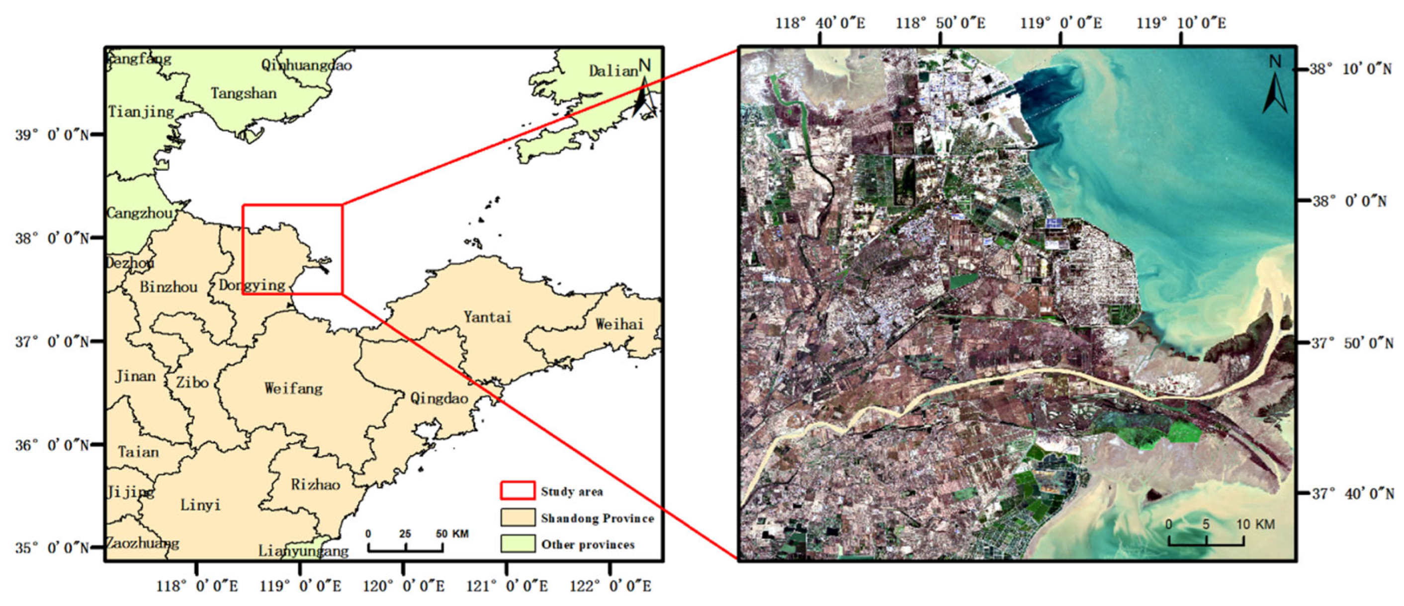
2.1. Study Area
2.2. Data Description
2.2.1. Sentinel-2 Data
2.2.2. Wetland Classification System
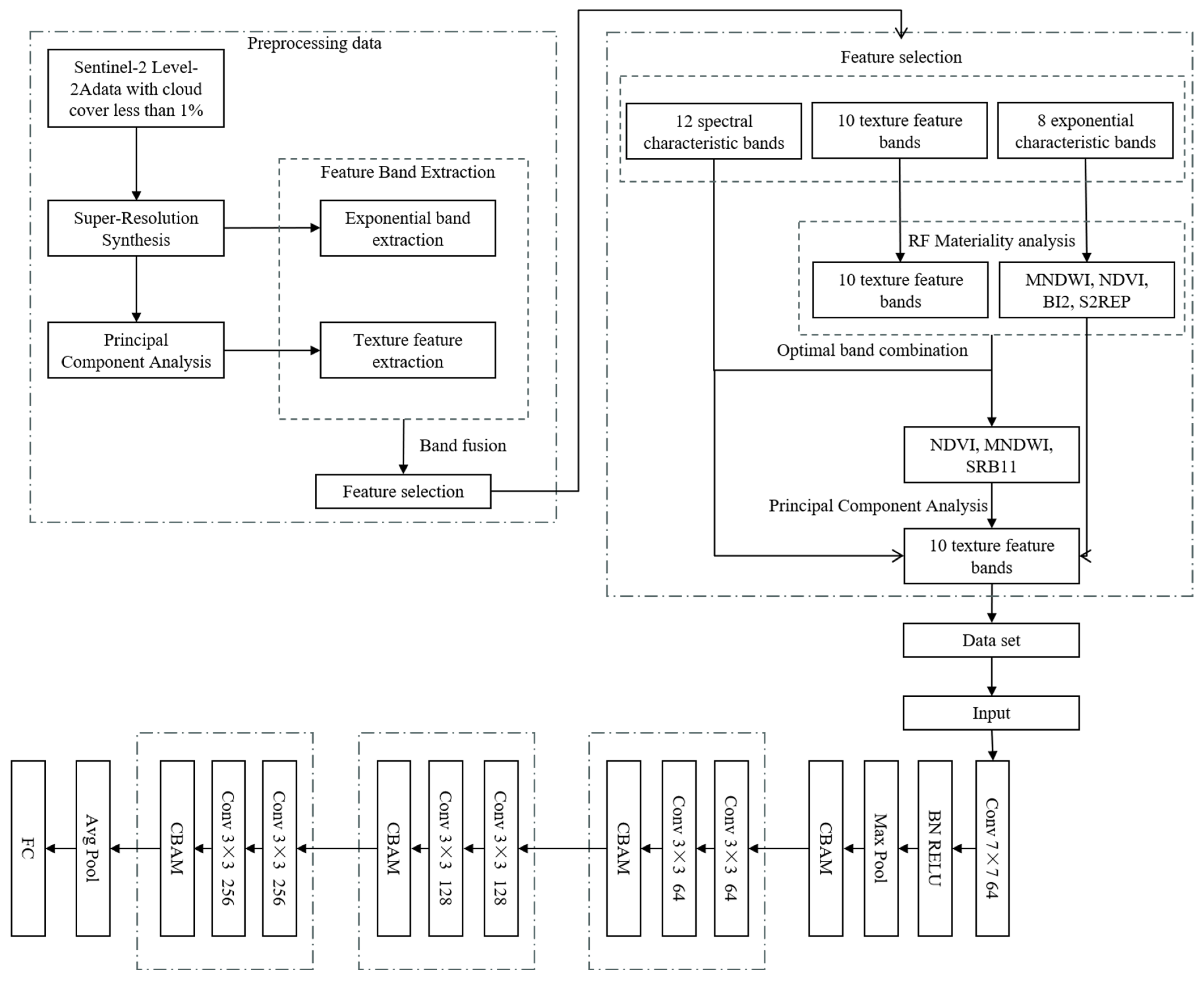
3. Methodology
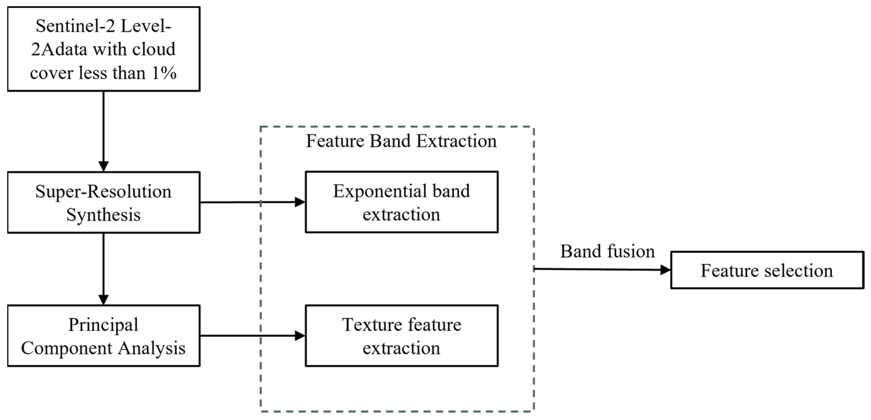
3.1. Data Preprocessing
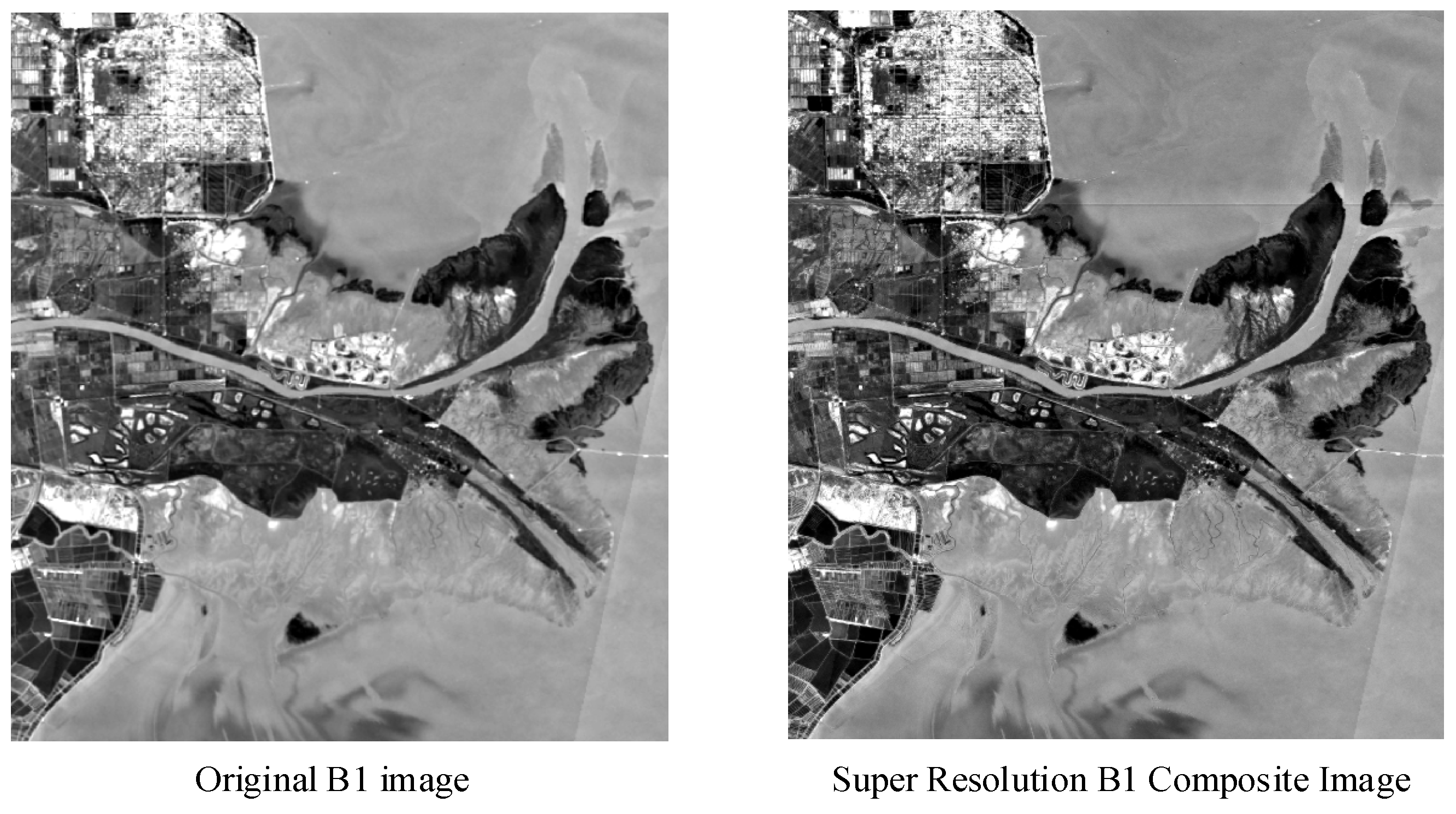
3.1.1. Super-Resolution Synthesis
3.1.2. Feature Band Extraction
3.2. Feature Extraction and Combination Scheme
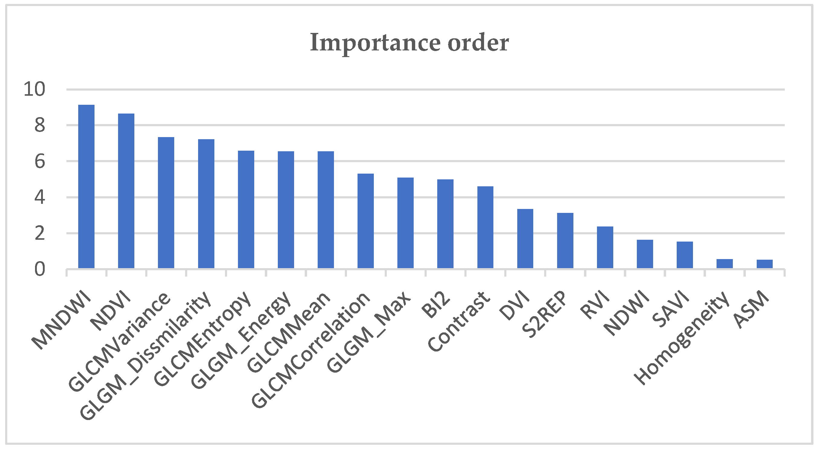
3.2.1. Band Importance Analysis
3.2.2. Combination Scheme
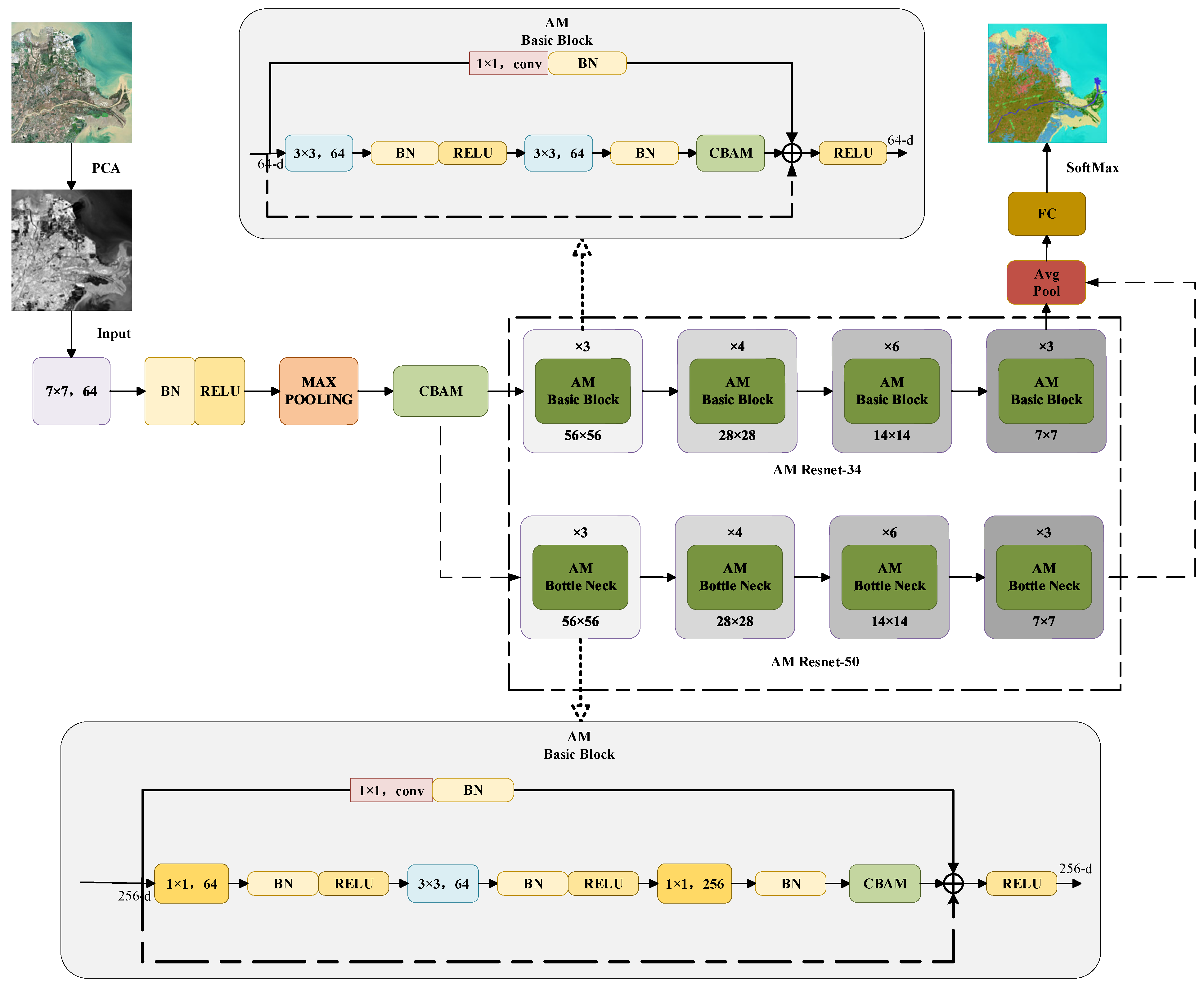
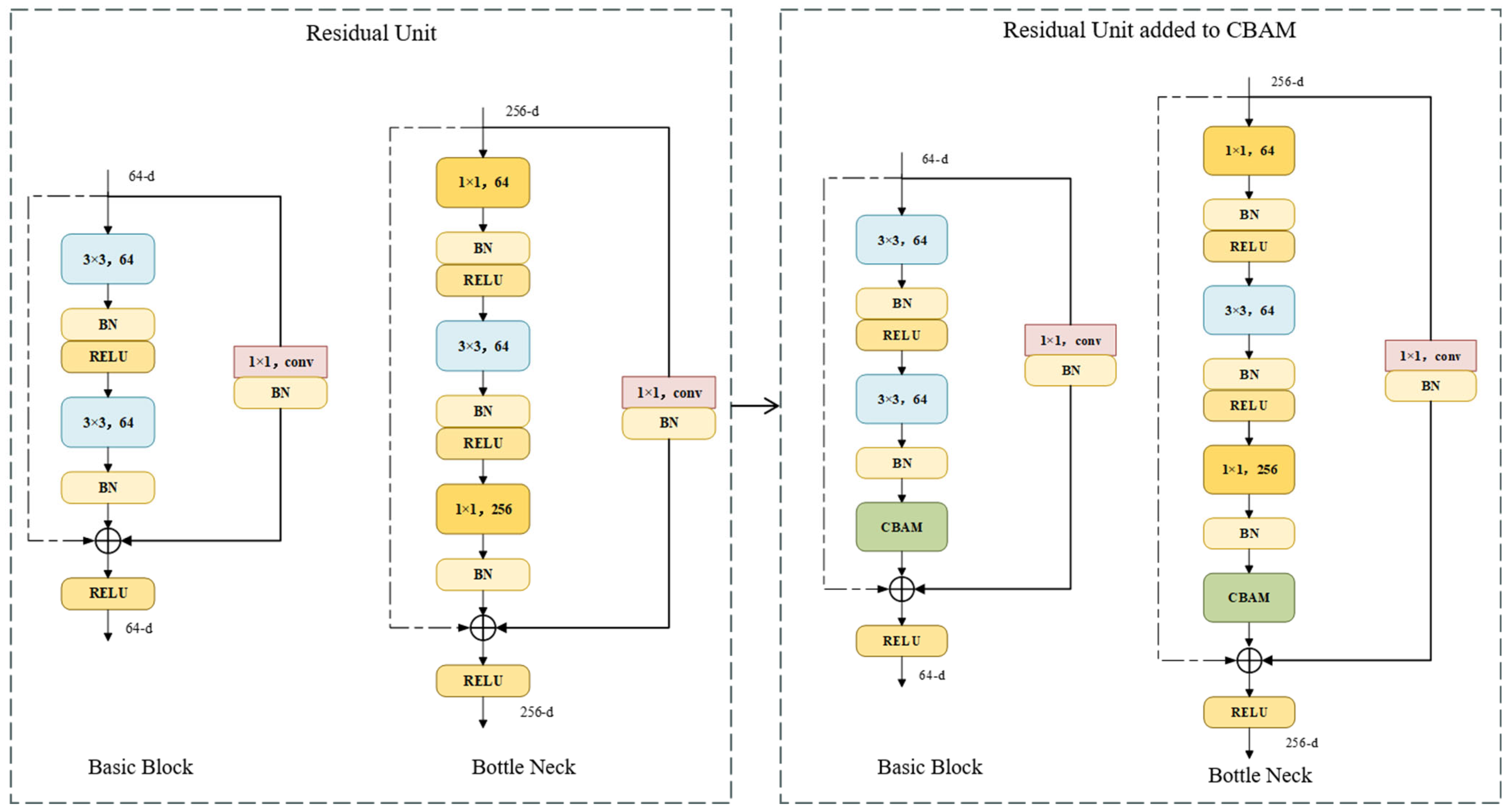
3.3. Attention Mechanism Combined with ResNet Network
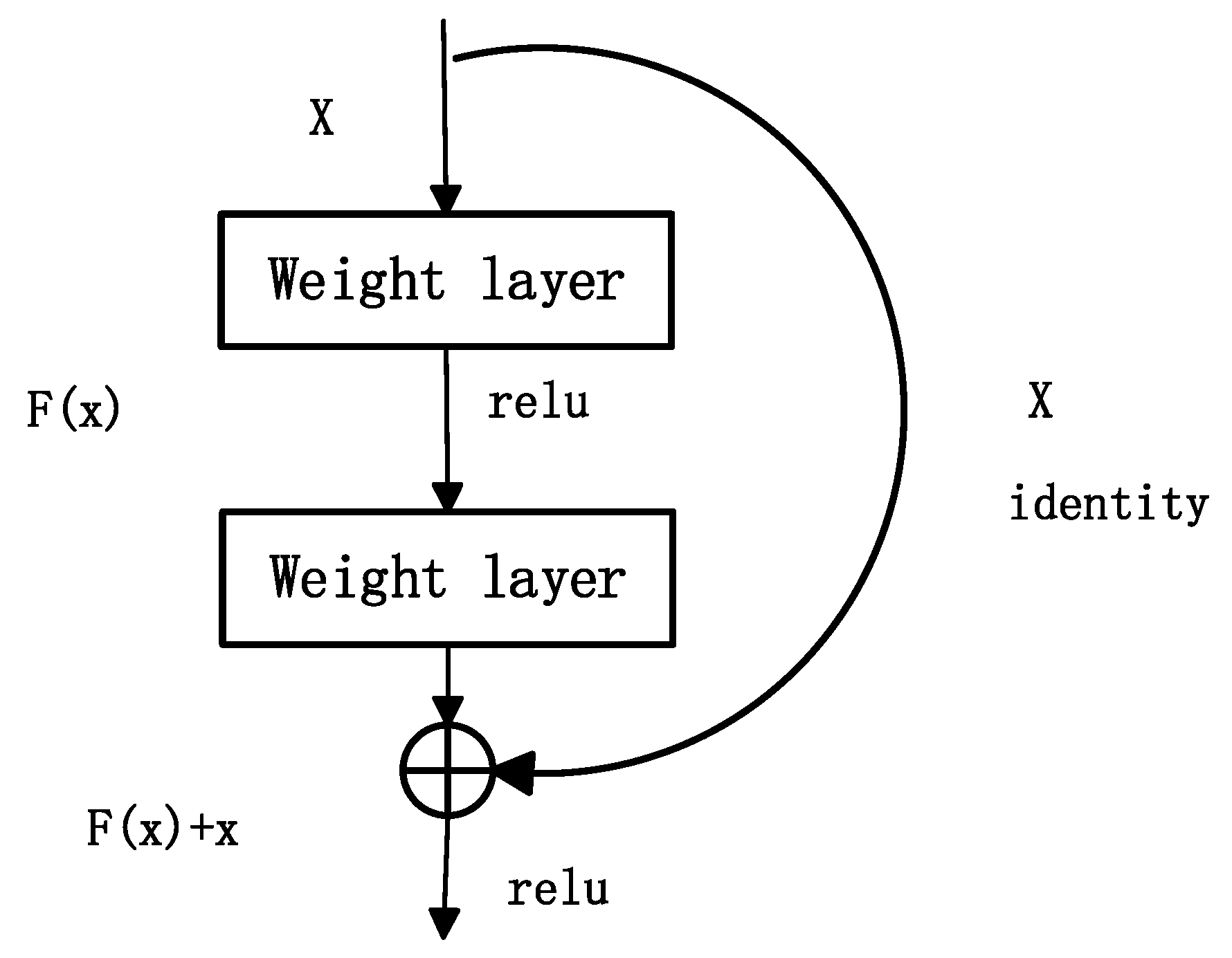
3.3.1. ResNet Network
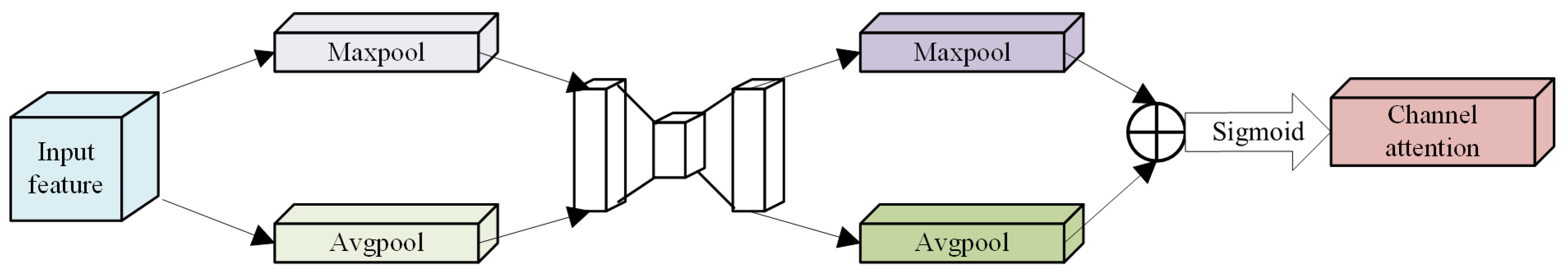
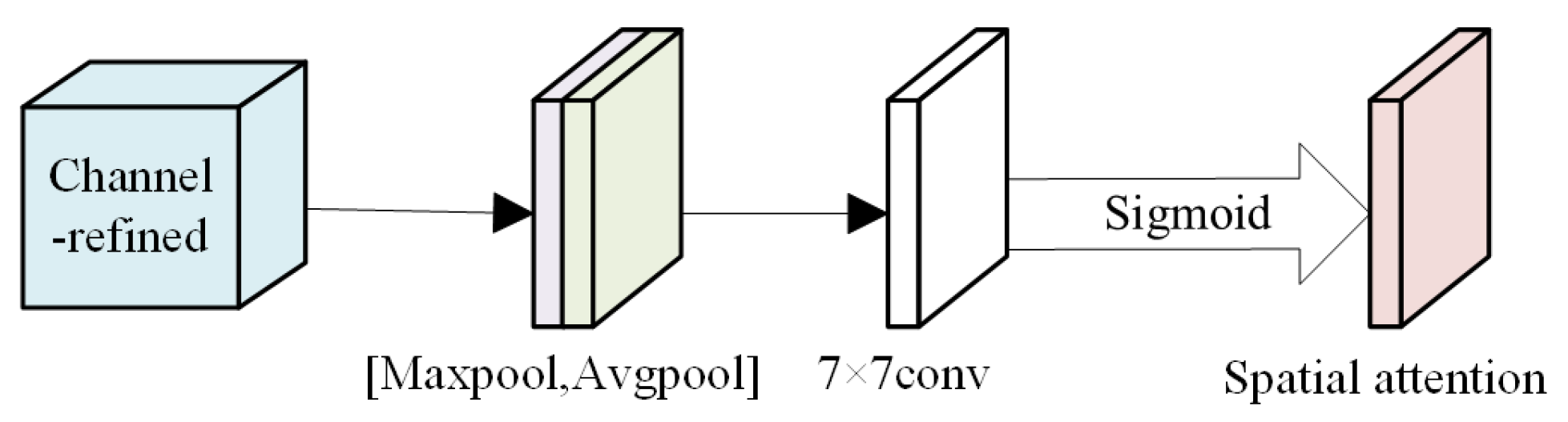
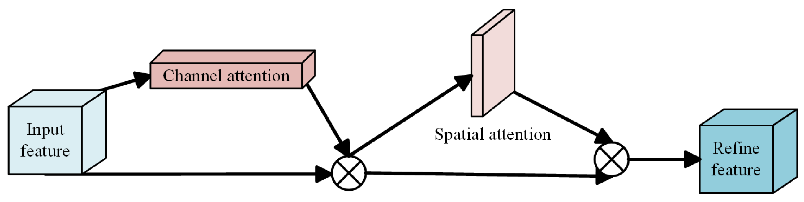
3.3.2. Attention Mechanism
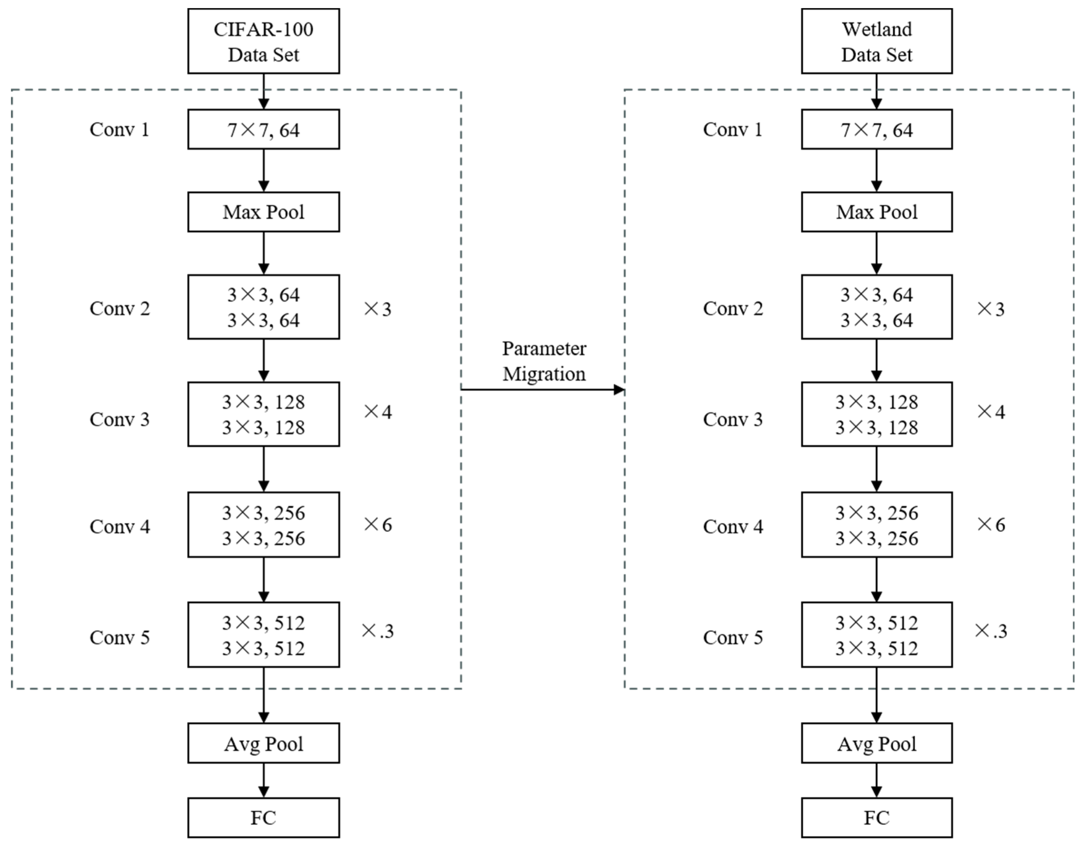
3.3.3. Transfer Learning
4. Classification Results and Accuracy Evaluation
4.1. Classification Effectiveness
4.2. Accuracy Evaluation
5. Discussion
5.1. Advantages of This Study
5.2. Limitations and Future Improvements
6. Conclusions
Author Contributions
Funding
Institutional Review Board Statement
Informed Consent Statement
Data Availability Statement
Conflicts of Interest
References
- Mitsch, W.J.; Gosselink, J.G. The Value of Wetlands: Importance of Scale and Landscape Setting. Ecol. Econ. 2000, 35, 25–33. [Google Scholar] [CrossRef]
- Zhang, X.; He, S.; Yang, Y. Evaluation of Wetland Ecosystem Services Value of the Yellow River Delta. Environ. Monit. Assess. 2021, 193, 353. [Google Scholar] [CrossRef] [PubMed]
- Liu, R.; Liang, S.; Zhao, H.; Qi, G.; Li, L.; Jiang, Y.; Niu, Z. Progress of Chinese Coastal Wetland Based on Remote Sensing. Remote Sens. Technol. Appl. 2017, 32, 998–1011. [Google Scholar]
- Wei, Z.; Jian, Z.; Sun, Y.; Pan, F.; Han, H.; Liu, Q.; Mei, Y. Ecological Sustainability and High-Quality Development of the Yellow River Delta in China Based on the Improved Ecological Footprint Model. Sci. Rep. 2023, 13, 3821. [Google Scholar] [CrossRef] [PubMed]
- Yan, J.; Zhu, J.; Zhao, S.; Su, F. Coastal Wetland Degradation and Ecosystem Service Value Change in the Yellow River Delta, China. Glob. Ecol. Conserv. 2023, 44, e02501. [Google Scholar] [CrossRef]
- Yu, B.; Zang, Y.; Wu, C.; Zhao, Z. Spatiotemporal Dynamics of Wetlands and Their Future Multi-Scenario Simulation in the Yellow River Delta, China. J. Environ. Manag. 2024, 353, 120193. [Google Scholar] [CrossRef] [PubMed]
- Liu, L.; Wang, H.; Yue, Q. China’s Coastal Wetlands: Ecological Challenges, Restoration, and Management Suggestions. Reg. Stud. Mar. Sci. 2020, 37, 101337. [Google Scholar] [CrossRef]
- Fu, Y.; Chen, S.; Ji, H.; Fan, Y.; Li, P. The Modern Yellow River Delta in Transition: Causes and Implications. Mar. Geol. 2021, 436, 106476. [Google Scholar] [CrossRef]
- Jia, Y.-Y.; Tang, L.; Li, C.; Yuan, X.; Qian, Y. Current Status and Development of Remote Sensing Technology Standardization in China. In Proceedings of the 2012 IEEE International Geoscience and Remote Sensing Symposium, Munich, Germany, 22–27 July 2012; IEEE: Munich, Germany, 2012; pp. 2775–2777. [Google Scholar]
- Huadong, G.; Changlin, W. Building up National Earth Observing System in China. Int. J. Appl. Earth Obs. Geoinf. 2005, 6, 167–176. [Google Scholar] [CrossRef]
- Bing, Z. Current Status and Future Prospects of Remote Sensing. Bull. Chin. Acad. Sci. 2017, 32, 12. [Google Scholar] [CrossRef]
- Aslam, R.W.; Shu, H.; Javid, K.; Pervaiz, S.; Mustafa, F.; Raza, D.; Ahmed, B.; Quddoos, A.; Al-Ahmadi, S.; Hatamleh, W.A. Wetland Identification through Remote Sensing: Insights into Wetness, Greenness, Turbidity, Temperature, and Changing Landscapes. Big Data Res. 2023, 35, 100416. [Google Scholar] [CrossRef]
- Zhu, Q.; Zhong, Y.; Zhang, L. Multi-Feature Probability Topic Scene Classifier for High Spatial Resolution Remote Sensing Imagery. In Proceedings of the 2014 IEEE Geoscience and Remote Sensing Symposium, Quebec City, QC, Canada, 13–18 July 2014; IEEE: Quebec City, QC, Canada, 2014; pp. 2854–2857. [Google Scholar]
- Xingyu, X.; Hongyu, L. Study on the Classification Approaches of Yancheng Coastal Wetlands based on ALOS Image. Remote Sens. Technol. Appl. 2013, 27, 248–255. [Google Scholar]
- Wu, Z.; Zhang, J.; Deng, F.; Zhang, S.; Zhang, D.; Xun, L.; Javed, T.; Liu, G.; Liu, D.; Ji, M. Fusion of GF and MODIS Data for Regional-Scale Grassland Community Classification with EVI2 Time-Series and Phenological Features. Remote Sens. 2021, 13, 835. [Google Scholar] [CrossRef]
- Bai, Y.; Sun, G.; Li, Y.; Ma, P.; Li, G.; Zhang, Y. Comprehensively Analyzing Optical and Polarimetric SAR Features for Land-Use/Land-Cover Classification and Urban Vegetation Extraction in Highly-Dense Urban Area. Int. J. Appl. Earth Obs. Geoinf. 2021, 103, 102496. [Google Scholar] [CrossRef]
- Sheng, H.; Wei, J.; Hu, Y.; Xu, M.; Cui, J.; Zheng, H. Wetland Information Extraction Based on Multifeature Optimization of Multitemporal Sentinel-2 Images. Mar. Sci. 2023, 47, 105–112. [Google Scholar]
- Zheng, H.; Du, P.; Chen, J.; Xia, J.; Li, E.; Xu, Z.; Li, X.; Yokoya, N. Performance Evaluation of Downscaling Sentinel-2 Imagery for Land Use and Land Cover Classification by Spectral-Spatial Features. Remote Sens. 2017, 9, 1274. [Google Scholar] [CrossRef]
- Wang, X.; Gao, X.; Zhang, Y.; Fei, X.; Chen, Z.; Wang, J.; Zhang, Y.; Lu, X.; Zhao, H. Land-Cover Classification of Coastal Wetlands Using the RF Algorithm for Worldview-2 and Landsat 8 Images. Remote Sens. 2019, 11, 1927. [Google Scholar] [CrossRef]
- Cui, L.; Zhang, J.; Wu, Z.; Xun, L.; Wang, X.; Zhang, S.; Bai, Y.; Zhang, S.; Yang, S.; Liu, Q. Superpixel Segmentation Integrated Feature Subset Selection for Wetland Classification over Yellow River Delta. Environ. Sci. Pollut. Res. 2023, 30, 50796–50814. [Google Scholar] [CrossRef] [PubMed]
- Lin, X.; Cheng, Y.; Chen, G.; Chen, W.; Chen, R.; Gao, D.; Zhang, Y.; Wu, Y. Semantic Segmentation of China’s Coastal Wetlands Based on Sentinel-2 and Segformer. Remote Sens. 2023, 15, 3714. [Google Scholar] [CrossRef]
- Lin, Z.; Wang, J.; Li, W.; Jiang, X.; Zhu, W.; Ma, Y.; Wang, A. OBH-RSI: Object-Based Hierarchical Classifica-Tion Using Remote Sensing Indices for Coastal Wetland. J. Beijing Inst. Technol. 2021, 30, 159–171. [Google Scholar] [CrossRef]
- Li, Y.; Zhang, H.; Xue, X.; Jiang, Y.; Shen, Q. Deep Learning for Remote Sensing Image Classification: A Survey. WIREs Data Min. Knowl. Discov. 2018, 8, e1264. [Google Scholar] [CrossRef]
- Zhu, X.X.; Tuia, D.; Mou, L.; Xia, G.-S.; Zhang, L.; Xu, F.; Fraundorfer, F. Deep Learning in Remote Sensing: A Comprehensive Review and List of Resources. IEEE Geosci. Remote Sens. Mag. 2017, 5, 8–36. [Google Scholar] [CrossRef]
- Mahdianpari, M.; Rezaee, M.; Zhang, Y.; Salehi, B. Wetland Classification Using Deep Convolutional Neural Network. In Proceedings of the IGARSS 2018—2018 IEEE International Geoscience and Remote Sensing Symposium, Valencia, Spain, 22–27 July 2018; IEEE: Valencia, Spain, 2018; pp. 9249–9252. [Google Scholar]
- Jamali, A.; Mahdianpari, M. Swin Transformer and Deep Convolutional Neural Networks for Coastal Wetland Classification Using Sentinel-1, Sentinel-2, and LiDAR Data. Remote Sens. 2022, 14, 359. [Google Scholar] [CrossRef]
- Jamali, A.; Mahdianpari, M.; Mohammadimanesh, F.; Brisco, B.; Salehi, B. 3-D Hybrid CNN Combined with 3-D Generative Adversarial Network for Wetland Classification with Limited Training Data. IEEE J. Sel. Top. Appl. Earth Obs. Remote Sens. 2022, 15, 8095–8108. [Google Scholar] [CrossRef]
- Li, X.-C.; Zhan, D.-C.; Yang, J.-Q.; Shi, Y.; Hang, C.; Lu, Y. Towards Understanding Transfer Learning Algorithms Using Meta Transfer Features. In Advances in Knowledge Discovery and Data Mining; Springer: Cham, Switzerland, 2020; pp. 855–866. [Google Scholar]
- Lu, J.; Behbood, V.; Hao, P.; Zuo, H.; Xue, S.; Zhang, G. Transfer Learning Using Computational Intelligence: A Survey. Knowl.-Based Syst. 2015, 80, 14–23. [Google Scholar] [CrossRef]
- He, K.; Zhang, X.; Ren, S.; Sun, J. Deep Residual Learning for Image Recognition. In Proceedings of the 2016 IEEE Conference on Computer Vision and Pattern Recognition (CVPR), Las Vegas, NV, USA, 27–30 June 2016; IEEE: Las Vegas, NV, USA, 2016; pp. 770–778. [Google Scholar]
- Alp, G.; Sertel, E. Deep Learning Based Patch-Wise Land Cover Land Use Classification: A New Small Benchmark Sentinel-2 Image Dataset. In Proceedings of the IGARSS 2022—2022 IEEE International Geoscience and Remote Sensing Symposium, Kuala Lumpur, Malaysia, 17–22 July 2022; IEEE: Kuala Lumpur, Malaysia, 2022; pp. 3179–3182. [Google Scholar]
- Naushad, R.; Kaur, T.; Ghaderpour, E. Deep Transfer Learning for Land Use and Land Cover Classification: A Comparative Study. Sensors 2021, 21, 8083. [Google Scholar] [CrossRef] [PubMed]
- Brauwers, G.; Frasincar, F. A General Survey on Attention Mechanisms in Deep Learning. IEEE Trans. Knowl. Data Eng. 2023, 35, 3279–3298. [Google Scholar] [CrossRef]
- Duan, S.; Zhao, J.; Huang, X.; Zhao, S. Semantic Segmentation of Remote Sensing Data Based on Channel Attention and Feature Information Entropy. Sensors 2024, 24, 1324. [Google Scholar] [CrossRef]
- Zhang, H.; Liu, S. Double-Branch Multi-Scale Contextual Network: A Model for Multi-Scale Street Tree Segmentation in High-Resolution Remote Sensing Images. Sensors 2024, 24, 1110. [Google Scholar] [CrossRef]
- Jiang, W.; Li, J.; Wang, W.; Xie, Z.; Mai, S. Assessment of Wetland Ecosystem Health Based on RS and GIS in Liaohe River Delta. In Proceedings of the 2005 IEEE International Geoscience and Remote Sensing Symposium, 2005—IGARSS ’05, Seoul, Republic of Korea, 29 July 2005; IEEE: Seoul, Republic of Korea, 2005; Volume 4, pp. 2384–2386. [Google Scholar]
- Drusch, M.; Del Bello, U.; Carlier, S.; Colin, O.; Fernandez, V.; Gascon, F.; Hoersch, B.; Isola, C.; Laberinti, P.; Martimort, P.; et al. Sentinel-2: ESA’s Optical High-Resolution Mission for GMES Operational Services. Remote Sens. Environ. 2012, 120, 25–36. [Google Scholar] [CrossRef]
- Xu, L.; Su, T.; Lei, B.; Wang, R.; Liu, X.; Meng, C.; Qi, J. The method of algal bloom extraction in Lake Chaohu waters based on FAI-L method. J. Lake Sci. 2023, 35, 1222–1233. [Google Scholar] [CrossRef]
- Tian, Y.; Chen, Z.; Hui, F.; Cheng, X.; Ouyang, L. ESA Sentinel-2A/B satellite: Characteristics and applications. J. Beijing Norm. Univ. Sci. 2019, 55, 57. [Google Scholar] [CrossRef]
- Li, Y.F.; Liu, H.Y. Advances in wetland classification and wetland landscape classification. Wetl. Sci. 2014, 12, 102–108. [Google Scholar] [CrossRef]
- Mao, D.; Wang, Z.; Du, B.; Li, L.; Tian, Y.; Jia, M.; Zeng, Y.; Song, K.; Jiang, M.; Wang, Y. National Wetland Mapping in China: A New Product Resulting from Object-Based and Hierarchical Classification of Landsat 8 OLI Images. ISPRS J. Photogramm. Remote Sens. 2020, 164, 11–25. [Google Scholar] [CrossRef]
- Panagiotopoulou, A.; Charou, E.; Stefouli, M.; Platis, K.; Madamopoulos, N.; Bratsolis, E. Sentinel-2 “Low Resolution Band” Optimization Using Super-Resolution Techniques: Lysimachia Lake Pilot Area of Analysis. In Proceedings of the 2019 10th International Conference on Information, Intelligence, Systems and Applications (IISA), Patras, Greece, 15–17 July 2019; IEEE: Patras, Greece, 2019; pp. 1–2. [Google Scholar]
- Wang, X.; Hu, Q.; Cheng, Y.; Ma, J. Hyperspectral Image Super-Resolution Meets Deep Learning: A Survey and Perspective. IEEECAA J. Autom. Sin. 2023, 10, 1668–1691. [Google Scholar] [CrossRef]
- Brodu, N. Super-Resolving Multiresolution Images with Band-Independant Geometry of Multispectral Pixels. In IEEE Transactions on Geoscience and Remote Sensing; IEEE: Washington, DC, USA, 2017. [Google Scholar]
- Zeng, Y.; Hao, D.; Huete, A.; Dechant, B.; Berry, J.; Chen, J.M.; Joiner, J.; Frankenberg, C.; Bond-Lamberty, B. Optical Vegetation Indices for Monitoring Terrestrial Ecosystems Globally | Nature Reviews Earth & Environment. Available online: https://www.nature.com/articles/s43017-022-00298-5 (accessed on 5 January 2024).
- Dan, L.; Baosheng, W. Review of Water Body Information Extraction Based on Satellite Remote Sensing. J. Tsinghua Univ. Technol. 2020, 60, 147–161. [Google Scholar] [CrossRef]
- Li, H.; Huang, J.; Liang, Y.; Wang, H.; Zhang, Y. Evaluating the quality of ecological environment in Wuhan based on remote sensing ecological index. J. Yunnan Univ. Nat. Sci. Ed. 2020, 42, 81–90. [Google Scholar]
- Rosenfeld, A.; Kak, A.C. Digital Picture Processing, 2nd ed.; Morgan Kaufmann Publishers: San Mateo, CA, USA, 2014; Available online: https://www.oreilly.com/library/view/digital-picture-processing/9780323139915/ (accessed on 5 January 2024).
- Liu, H.Q.; Huete, A. A Feedback Based Modification of the NDVI to Minimize Canopy Background and Atmospheric Noise. In IEEE Transactions on Geoscience and Remote Sensing; IEEE: Piscataway, NJ, USA, 1995; Available online: https://ieeexplore.ieee.org/document/8746027 (accessed on 5 January 2024).
- Jordan, C.F. Derivation of Leaf-Area Index from Quality of Light on the Forest Floor. Ecology 1969, 50, 663–666. Available online: https://esajournals.onlinelibrary.wiley.com/doi/abs/10.2307/1936256 (accessed on 5 January 2024). [CrossRef]
- Epifanio, I. Intervention in Prediction Measure: A New Approach to Assessing Variable Importance for Random Forests. BMC Bioinform. 2017, 18, 230. [Google Scholar] [CrossRef]
- Rui, C.; Xue, W. Wavelength Selection Method of Near-Infrared Spectrum Based on Random Forest Feature Importance and Interval Partial Least Square Method. Spectrosc. Spectr. Anal. 2023, 43, 1043–1050. [Google Scholar]
- Zhao, L.; Li, Q.; Chang, Q.; Shang, J.; Du, X.; Liu, J.; Dong, T. In-Season Crop Type Identification Using Optimal Feature Knowledge Graph. ISPRS J. Photogramm. Remote Sens. 2022, 194, 250–266. [Google Scholar] [CrossRef]
- Acharya, T.; Yang, I.; Lee, D. Land-Cover Classification of Imagery from Landsat Operational Land Imager Based on Optimum Index Factor. Sens. Mater. 2018, 30, 1753–1764. [Google Scholar] [CrossRef]
- Kienast-Brown, S.; Boettinger, J.L. Applying the Optimum Index Factor to Multiple Data Types in Soil Survey. In Digital Soil Mapping; Boettinger, J.L., Howell, D.W., Moore, A.C., Hartemink, A.E., Kienast-Brown, S., Eds.; Springer: Dordrecht, The Netherlands, 2010; pp. 385–398. ISBN 978-90-481-8862-8. [Google Scholar]
- Glafkides, J.-P.; Sher, G.I.; Akdag, H. Phylogenetic Replay Learning in Deep Neural Networks. Jordanian J. Comput. Inf. Technol. 2022, 8, 112–126. [Google Scholar] [CrossRef]
- Vaswani, A.; Shazeer, N.; Parmar, N.; Uszkoreit, J.; Jones, L.; Gomez, A.N.; Kaiser, L.; Polosukhin, I. Attention Is All You Need. In Proceedings of the 31st Conference on Neural Information Processing Systems (NIPS 2017), Long Beach, CA, USA, 4–9 December 2017; pp. 6000–6010. [Google Scholar]
- Gao, G. Survey on Attention Mechanisms in Deep Learning Recommendation Models. Comput. Eng. Appl. 2022, 58, 9. [Google Scholar] [CrossRef]
- Woo, S.; Park, J.; Lee, J.-Y.; Kweon, I.S. CBAM: Convolutional Block Attention Module. In Computer Vision—ECCV 2018; Ferrari, V., Hebert, M., Sminchisescu, C., Weiss, Y., Eds.; Lecture Notes in Computer Science; Springer International Publishing: Cham, Switzerland, 2018; Volume 11211, pp. 3–19. ISBN 978-3-030-01233-5. [Google Scholar]
- Yang, Z.; Zhang, T.; Yang, J. Research on Classification Algorithms for Attention Mechanism. In Proceedings of the 2020 19th International Symposium on Distributed Computing and Applications for Business Engineering and Science (DCABES), Xuzhou, China, 16–19 October 2020; IEEE: Xuzhou, China, 2020; pp. 194–197. [Google Scholar]
- Weiss, K.; Khoshgoftaar, T. Evaluation of Transfer Learning Algorithms Using Different Base Learners. In Proceedings of the 2017 IEEE 29th International Conference on Tools with Artificial Intelligence (ICTAI), Boston, MA, USA, 6–8 November 2017; IEEE: Boston, MA, USA, 2017; pp. 187–196. [Google Scholar]
- Guo, J.; Han, K.; Wu, H.; Tang, Y.; Chen, X.; Wang, Y.; Xu, C. CMT: Convolutional Neural Networks Meet Vision Transformers. In Proceedings of the 2022 IEEE/CVF Conference on Computer Vision and Pattern Recognition (CVPR), New Orleans, LA, USA, 18–24 June 2022; pp. 12165–12175. [Google Scholar]
- Chen, J.; Lu, Y.; Yu, Q.; Luo, X.; Adeli, E.; Wang, Y.; Lu, L.; Yuille, A.L.; Zhou, Y. TransUNet: Transformers Make Strong Encoders for Medical Image Segmentation. arXiv 2021, arXiv:2102.04306. [Google Scholar] [CrossRef]


| Product Level | Product Introduction |
|---|---|
| Level-0 | Raw data |
| Level-1A | Geometric coarse correction products containing metainformation |
| Level-1B | Radiance product, embedded in a GCP-optimized geometric model but without the corresponding geometric corrections |
| Level-1C | Atmospheric apparent reflectance products after orthorectification and sub-image-level geometric refinement corrections |
| Level-2A | Contains primarily atmospherically corrected bottom-of-the-atmosphere reflectance data |
| Sensor | Band Number | Band Name | Sentinel-2A | Sentinel-2B | Resolution (Meters) | ||
|---|---|---|---|---|---|---|---|
| Central Wavelength (nm) | Bandwidth (nm) | Central Wavelength (nm) | Bandwidth (nm) | ||||
| MSI | 1 | Coastal aerosol | 443.9 | 20 | 442.3 | 20 | 60 |
| 2 | Blue | 496.6 | 65 | 492.1 | 65 | 10 | |
| 3 | Green | 560.0 | 35 | 559 | 35 | 10 | |
| 4 | Red | 664.5 | 30 | 665 | 30 | 10 | |
| 5 | Vegetation Red Edge | 703.9 | 15 | 703.8 | 15 | 20 | |
| 6 | Vegetation Red Edge | 740.2 | 15 | 739.1 | 15 | 20 | |
| 7 | Vegetation Red Edge | 782.5 | 20 | 779.7 | 20 | 20 | |
| 8 | NIR | 835.1 | 115 | 833 | 115 | 10 | |
| 8b | Narrow NIR | 864.8 | 20 | 864 | 20 | 20 | |
| 9 | Water vapor | 945.0 | 20 | 943.2 | 20 | 60 | |
| 10 | SWIR-Cirrus | 1373.5 | 30 | 1376.9 | 30 | 60 | |
| 11 | SWIR | 1613.7 | 90 | 1610.4 | 90 | 20 | |
| 12 | SWIR | 2202.4 | 180 | 2185.7 | 180 | 20 | |
| First Level Classification | Second Level Classification | Identification and Map Color | Legend | Classification Diagram |
|---|---|---|---|---|
| Natural wetlands | Shrub swamps | SS Dark green | 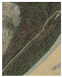 |  |
| Herbaceous swamp | HS Light green | 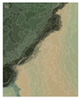 |  | |
| Rivers | RV Purple | 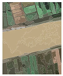 | 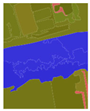 | |
| Mudflat | MF Light yellow | 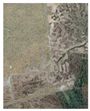 | 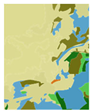 | |
| Artificial wetland | reservoir and pond | RE Light blue | 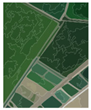 |  |
| Salt pan | SP orange |  |  | |
| Non-wetland | Construction land | CL Red | 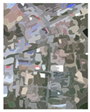 |  |
| Farmland | FA Brown |  |  | |
| Shallow water | SW Light blue |  |  | |
| Other land use | OL White |  |  |
| Feature Category | Feature Name | Feature Expression |
|---|---|---|
| Spectral characteristics | Band | Blue (B2), green (B3), red (B4), near-infrared (B8), red end (B5), near-infrared NIR (B6, B7, and B8A), shortwave infrared SWIR (B11 and B12), coastal atmospheric aerosols (B1), and cirrus bands (B10) |
| Vegetation/Water Index | NDVI [49] | |
| MNDWI | ||
| NDWI | ||
| REPI | ||
| DVI [50] | ||
| RVI | ||
| soil index | BI | |
| SAVI | ||
| Tasseled Cap | Brightness | |
| Greenness | ||
| Wetness | ||
| Texture Features | GLGM_Variance | |
| GLGM_Contrast | ||
| GLGM_Entropy | ||
| GLGM_Correlation | ||
| GLGM_Homogeneity | ||
| GLGM_ASM | ||
| GLGM_Mean | ||
| GLGM_Dissmilarity | ||
| GLGM_Energy | ||
| GLGM_Max |
| Evaluation Indicators | Calculation Methods | Explanations |
|---|---|---|
| User Accuracy (UA) | represents the number of correct classifications, represents the total number of categories. | |
| Producer Accuracy (PA) | represents the number of correct classifications, represents the total number of misclassifications to a certain category. | |
| F1-score | P stands for precision rate and R stands for with recall rate. | |
| Overall Accuracy (OA) | C represents the total number of categories, represents the number of correctly classified samples for each category, and n represents the total number of samples. | |
| KAPPA | represents the overall classification accuracy, , is the number of real samples for each category, is the number of predicted samples. |
| Method | OA(%) | Kappa | F1-Score | Accuracy | Category | |||||||||
|---|---|---|---|---|---|---|---|---|---|---|---|---|---|---|
| SW | MF | RV | HS | SS | RE | FA | SP | CL | OL | |||||
| SVM | 85.03 | 0.81 | 81.26 | PA | 84.33 | 83.21 | 86.03 | 78.93 | 84.54 | 79.89 | 87.05 | 89.13 | 87.72 | 85.56 |
| UA | 88.87 | 87.46 | 85.81 | 82.35 | 85.73 | 81.02 | 86.36 | 87.79 | 90.02 | 81.06 | ||||
| RF | 87.62 | 0.83 | 84.55 | PA | 86.2 | 86.4 | 86.68 | 69.15 | 89.27 | 80.9 | 90.53 | 94.44 | 91.8 | 88.67 |
| UA | 93.82 | 93.79 | 92.74 | 66.97 | 83.79 | 85 | 93.78 | 96.9 | 74.74 | 94.25 | ||||
| ResNet34 | 92.59 | 0.91 | 90.62 | PA | 94.59 | 92.29 | 93.85 | 82.07 | 82.16 | 89.38 | 94.33 | 93.18 | 91.81 | 93.86 |
| UA | 94.92 | 92.03 | 94.09 | 85.92 | 85.02 | 94.08 | 97.18 | 95.67 | 65.15 | 92.95 | ||||
| ResNet50 | 91.77 | 0.9 | 89.43 | PA | 94.44 | 94.15 | 93.71 | 89.86 | 89.74 | 85.88 | 90.65 | 95.15 | 87.65 | 91.65 |
| UA | 96.59 | 91.45 | 96.29 | 94.66 | 94.27 | 91.76 | 93.59 | 96.94 | 71.65 | 95.65 | ||||
| AR34 | 93.76 | 0.92 | 91.02 | PA | 94.04 | 95.37 | 94.86 | 91.17 | 92.14 | 90.48 | 94.45 | 97.43 | 91.56 | 95.11 |
| UA | 93.52 | 94.08 | 96.46 | 95.24 | 95.26 | 93.75 | 91.02 | 92.43 | 84.58 | 96.46 | ||||
| AR50 | 94.61 | 0.93 | 91.93 | PA | 95.2 | 94.48 | 93.91 | 92.73 | 92.38 | 90.31 | 96.29 | 97.68 | 93.37 | 94.35 |
| UA | 94.64 | 93.63 | 95.59 | 94.52 | 94.52 | 95.49 | 92.48 | 91.32 | 85.25 | 95.85 | ||||
Disclaimer/Publisher’s Note: The statements, opinions and data contained in all publications are solely those of the individual author(s) and contributor(s) and not of MDPI and/or the editor(s). MDPI and/or the editor(s) disclaim responsibility for any injury to people or property resulting from any ideas, methods, instructions or products referred to in the content. |
© 2024 by the authors. Licensee MDPI, Basel, Switzerland. This article is an open access article distributed under the terms and conditions of the Creative Commons Attribution (CC BY) license (https://creativecommons.org/licenses/by/4.0/).
Share and Cite
Li, Y.; Yu, X.; Zhang, J.; Zhang, S.; Wang, X.; Kong, D.; Yao, L.; Lu, H. Improved Classification of Coastal Wetlands in Yellow River Delta of China Using ResNet Combined with Feature-Preferred Bands Based on Attention Mechanism. Remote Sens. 2024, 16, 1860. https://doi.org/10.3390/rs16111860
Li Y, Yu X, Zhang J, Zhang S, Wang X, Kong D, Yao L, Lu H. Improved Classification of Coastal Wetlands in Yellow River Delta of China Using ResNet Combined with Feature-Preferred Bands Based on Attention Mechanism. Remote Sensing. 2024; 16(11):1860. https://doi.org/10.3390/rs16111860
Chicago/Turabian StyleLi, Yirong, Xiang Yu, Jiahua Zhang, Shichao Zhang, Xiaopeng Wang, Delong Kong, Lulu Yao, and He Lu. 2024. "Improved Classification of Coastal Wetlands in Yellow River Delta of China Using ResNet Combined with Feature-Preferred Bands Based on Attention Mechanism" Remote Sensing 16, no. 11: 1860. https://doi.org/10.3390/rs16111860
APA StyleLi, Y., Yu, X., Zhang, J., Zhang, S., Wang, X., Kong, D., Yao, L., & Lu, H. (2024). Improved Classification of Coastal Wetlands in Yellow River Delta of China Using ResNet Combined with Feature-Preferred Bands Based on Attention Mechanism. Remote Sensing, 16(11), 1860. https://doi.org/10.3390/rs16111860