Enhanced Wind Field Spatial Downscaling Method Using UNET Architecture and Dual Cross-Attention Mechanism

Abstract

Before 2008, China lacked high-coverage regional surface observation data, making it difficult for the China Meteorological Administration Land Data Assimilation System (CLDAS) to directly backtrack high-resolution, high-quality land assimilation products. To address this issue, this paper proposes a deep learning model named UNET_DCA, based on the UNET architecture, which incorporates a Dual Cross-Attention module (DCA) for multiscale feature fusion by introducing Channel Cross-Attention (CCA) and Spatial Cross-Attention (SCA) mechanisms. This model focuses on the near-surface 10-m wind field and achieves spatial downscaling from 6.25 km to 1 km. We conducted training and validation using data from 2020–2021, tested with data from 2019, and performed ablation experiments to validate the effectiveness of each module. We compared the results with traditional bilinear interpolation methods and the SNCA-CLDASSD model. The experimental results show that the UNET-based model outperforms SNCA-CLDASSD, indicating that the UNET-based model captures richer information in wind field downscaling compared to SNCA-CLDASSD, which relies on sequentially stacked CNN convolution modules. UNET_CCA and UNET_SCA, incorporating cross-attention mechanisms, outperform UNET without attention mechanisms. Furthermore, UNET_DCA, incorporating both Channel Cross-Attention and Spatial Cross-Attention mechanisms, outperforms UNET_CCA and UNET_SCA, which only incorporate one attention mechanism. UNET_DCA performs best on the RMSE, MAE, and COR metrics (0.40 m/s, 0.28 m/s, 0.93), while UNET_DCA_ars, incorporating more auxiliary information, performs best on the PSNR and SSIM metrics (29.006, 0.880). Evaluation across different methods indicates that the optimal model performs best in valleys, followed by mountains, and worst in plains; it performs worse during the day and better at night; and as wind speed levels increase, accuracy decreases. Overall, among various downscaling methods, UNET_DCA and UNET_DCA_ars effectively reconstruct the spatial details of wind fields, providing a deeper exploration for the inversion of high-resolution historical meteorological grid data.

1. Introduction

The China Meteorological Administration’s high-resolution land data assimilation system (CLDAS3.0) [1] utilizes data assimilation techniques to integrate various meteorological observation data, surface feature data, and outputs from numerical weather prediction models to generate high-quality assimilation products with an hourly spatial resolution of 1 km. However, before 2008, China lacked high-coverage regional surface observation data, making it difficult for CLDAS3.0 to directly backtrack high-resolution, high-quality land assimilation products. Spatial downscaling methods can address this issue. Currently, spatial downscaling methods mainly consist of dynamic downscaling and statistical downscaling. Dynamic downscaling is a physically-based method that simulates and resolves the dynamic processes of the atmospheric system to transform lower-resolution meteorological data into higher-resolution data. Its advantages lie in strong physical interpretability and high predictability, but it incurs high computational costs and uncertainty at high resolutions [2,3,4]. Statistical downscaling, on the other hand, is a statistical method that establishes mapping relationships between high-resolution and low-resolution data to achieve spatial scale transformation from coarse to fine granularity. It is relatively simple, computationally efficient, and offers greater flexibility in terms of the study area and specific implementation schemes. Consequently, it has been widely applied in regional climate simulation and prediction [5,6,7,8,9,10].

In recent years, deep learning technology has provided new insights for improving the accuracy of statistical downscaling results. Among them, image super-resolution based on deep learning is an important image reconstruction technique in computer vision image processing. Its aim is to recover high-resolution images from low-resolution ones, with wide applications in medical imaging, satellite image remote sensing, video restoration, and 3D rendering [11,12,13,14]. Increasingly, research has demonstrated that end-to-end image super-resolution algorithms can be effectively migrated to meteorological element downscaling to improve accuracy [15,16,17,18]. In 2017, Vandal et al. [19] first applied super-resolution technology to the field of meteorological downscaling, proposing a deep learning model named DeepSD based on stacked super-resolution convolutional neural network (SRCNN) modules. In experiments downsizing daily precipitation over the contiguous United States, DeepSD exhibited better performance than traditional dynamic and statistical downscaling methods. In 2019, Mao Renzhi [20] addressed the shallow depth of the DeepSD network and its inability to handle non-integer scaling, proposing enhanced deep downscaling models VDSD (Very Deep Statistical Downscaling) and ResSD (Statistical Downscaling using Residual Convolutional Network). In experiments downsizing precipitation fields in the Chinese region, the results showed superior TS scores compared to DeepSD. In 2022, Tie Ruian et al. [21] innovatively introduced the CLDASSD model based on VDSD, incorporating global skip connections and attention mechanisms. Experimental results demonstrated the model’s stronger spatial reconstruction capabilities in temperature fields over mountainous regions. In the same year, Tie Ruian [22] improved the complexity, parameter count, and loss function of the CLDASSD model, proposing the Light-CLDASSD model. Experimental results showed that all indicators outperformed bilinear interpolation, DeepSD, and CLDASSD, demonstrating its ability to capture small-scale temperature field distribution characteristics in plains areas. In 2023, Shen Zhanfei [23] improved the modules of Light-CLDASSD and proposed an SNCA-CLDASSD model utilizing shuffle-nonlinear activation blocks (SNBlock), Spatial Cross-Attention mechanisms (SCAMs), and content-aware feature rearrangement upsampling (CARAFE). This model exhibited better robustness, effectively suppressed the checkerboard effect, and could reconstruct spatial texture details of 2 m temperature fields more clearly.

The neural network structures in the above methods are all sequentially stacked CNN convolutional blocks, some of which incorporate residual modules, attention mechanisms, or improved downsampling and upsampling modules to enhance the performance of the network model. The drawback of such models lies in the local nature of convolutions, which leads to the easy loss of feature information during downsampling, thereby failing to capture long-range dependencies between different features. Consequently, scholars have attempted to improve the performance of downsizing based on the UNET architecture. For example, in 2020, Höhlein et al. [24] established the DeepRU model based on the UNET architecture, addressing the issue of traditional CNN algorithms failing to reconstruct the wind field structure. In 2023, Dupuy et al. [25] utilized the UNET architecture to downscale near-surface wind fields using two improved mean squared error (MSE) loss functions, with experimental results demonstrating optimal improvements in wind speed or direction, and combining the two models yielded the best overall performance. In the same year, Lin et al. [26] applied the UNET downsizing method and bias correction to develop the East Asia high-resolution dataset (CLIMEA-BCUD), with validation results indicating that the dataset performs reasonably in climatology, effectively simulating seasonal cycles and future changes. Numerous scientific experiments have demonstrated that the multi-level feature extraction and skip connections of the UNET architecture can integrate features at large and small scales, thereby learning high-level semantic and low-level detailed features and aiding in the model’s understanding of complex structures within images.

Building upon prior research, this study considers the complex interaction between large-scale wind fields and small-scale boundary layers in ground wind fields. Therefore, the efficient extraction and integration of the large-scale and small-scale features of both wind fields and terrain significantly impact the accuracy of the spatial downsizing of wind fields. In order to better reconstruct the wind field, this paper focuses on how to better learn the relationship between wind fields and terrain at different scales. Therefore, based on the UNET architecture, this research is conducted. However, it also has some shortcomings. For instance, simple skip connections in encoder and decoder features can lead to semantic gaps. Inspired by achievements in the field of medical image segmentation [27,28,29], this paper introduces a Dual Cross-Attention module (DCA) based on the UNET architecture, incorporating Channel Cross-Attention (CCA) and Spatial Cross-Attention (SCA) mechanisms. This DCA module adaptively captures channel and spatial dependencies between multi-scale encoder features in sequence to address the semantic gaps between encoder and decoder features in the UNET architecture. This is aimed at better learning information at different spatial scales, establishing a deep learning model based on the UNET architecture and the Dual Cross-Attention mechanism (DCA). The goal is to achieve the spatial downsizing of near-surface 10 m wind field product data from 0.0625° (coarse scale) to 0.01° (fine scale) within the China Meteorological Administration Land Data Assimilation System (CLDAS), reconstructing high-resolution, high-quality land assimilation products before 2008, and filling the historical gap in CLDAS3.0 before 2008. In this study, 80% of the data from 2020–2021 is used for training, 20% for validation, and data from 2019 is used for testing. Ablation experiments are conducted to verify the effectiveness of each module, and comparisons are made with traditional bilinear interpolation methods and SNCA-CLDASSD, which has shown excellent performance in spatial downscaling of ground-level 2 m temperature. The results indicate that the UNET_DCA model, which incorporates a Dual Cross-Attention mechanism, exhibits the best performance in terms of RMSE, MAE, and COR metrics. Furthermore, the UNET_DCA_ars model, which incorporates additional auxiliary information, achieves optimal performance in the PSNR and SSIM indicators.

Section 2 of this paper primarily delineates the study area, the dataset utilized, and the data processing methodology. Moving on to Section 3, a comprehensive exposition will be provided on the structure, principles, and functionalities of each module within the downscaling model. Subsequently, Section 4 will outline the testing scheme for the ablation experiment and the evaluation metrics employed to assess the model’s performance. In Section 5, a meticulous analysis of the experimental results for each model will be presented.

2. Data and Processing

2.1. Study Area

The study area (as shown in Figure 1) covers a longitude range of 109.0° to 116.0°E and a latitude range of 34.0° to 41.0°N, including Shanxi Province and its surrounding areas. The region exhibits diverse ground features and complex terrain, including mountains, plateaus, basins, river valleys, and plains. Most of the area is mountainous, primarily located in the western and eastern parts of Shanxi Province. Plateaus are mainly distributed in the northwest of the study area and the southwest of Shanxi Province. Basins are found in the intermediate zone between the mountain ranges on both sides of Shanxi Province. River valleys are located in the region where Shanxi and Shaanxi provinces intersect, along the Yellow River. The plains are situated in the southeastern part of the study area. The study area belongs to the warm temperate monsoon climate zone. The spring and winter seasons experience relatively strong winds, particularly the north wind during the winter. In the summer, the region is influenced by warm and moist air currents, resulting in high temperatures and abundant precipitation. In contrast, winter is influenced by cold and dry air currents, leading to low temperatures and less precipitation.

Based on the characteristics of the underlying surface, the study area is segmented into five distinct terrains: mountain, plateau, basin, valley, and plain.

Table 1. The numbers of the five terrains in the 49 small areas divided by the right figure in Figure 1.

Topography	Serial Number
Mountains	4, 5, 6, 7, 8, 9, 10, 11, 12, 13, 14, 15, 17, 18, 19, 22, 24, 26, 29, 32, 33, 36
Highland	1, 2, 3, 39, 45, 46
Basin	25, 31, 37, 38, 43, 44
Valley	16, 23, 30
Plain	20, 21, 27, 28, 34, 35, 40, 41, 42, 47, 48, 49

displays the numerical distribution of these small areas, corresponding to the five different terrains.

2.2. Data

Table 2 enumerates all the data employed in this study. The hourly data for the years 2020 and 2021 are partitioned into training sets (80%) and validation sets (20%), with the data from 2019 designated for independent testing. Additionally, Digital Elevation Model (DEM) data are incorporated as auxiliary information during the training phase. Table 2 presents all the data used in this study. The hourly data from 2020 and 2021 were randomly shuffled and divided into a training set (80%) and a validation set (20%), while the data from 2019 serve as an independent test set. During the training phase, a Digital Elevation Model (DEM) was introduced as auxiliary data. The following sections provide a detailed introduction to each type of data.

(1)

CLDAS-V2.0 data [30], provided by the National Meteorological Information Center of the China Meteorological Administration, is coarse-resolution land surface data used as input for the model in this study. This data are generated by assimilating various ground and satellite observations using techniques such as the Spatial and Temporal Multiscale Analysis System (STMAS), Cumulative Distribution Function (CDF) matching, physical inversion, and terrain correction. It produces hourly, 0.0625° spatiotemporal resolution products covering the Asian region (0–60°N, 70–140°E). Compared to similar products, CLDAS-V2.0 data exhibit superior quality and has been widely applied in meteorological and environmental research fields. Each individual grid of the low-resolution wind field in the study area measures 112 × 112.

(2)

CLDAS-V3.0 product [1], high-resolution land surface data from the National Meteorological Information Center of the China Meteorological Administration, is used as the label data for the model in this study. This product combines the weather forecast products from the European Centre for Medium-Range Weather Forecasts (ECMWF) with over 60,000 national and regional automatic weather station data deployed by the China Meteorological Administration using the Spatial and Temporal Multiscale Analysis System (STMAS) assimilation method. It generates hourly, 0.01° spatiotemporal resolution merged data on an equally spaced latitude-longitude land grid, providing more detailed and accurate land surface meteorological information such as temperature, humidity, wind speed, and precipitation with higher spatiotemporal resolution. The grid size of each high-resolution wind field label in the study area is 700 × 700.

(3)

DEM data, obtained from a joint mapping mission called the Shuttle Radar Topography Mission (SRTM) conducted by the United States, Germany, and Italy’s national space agencies, is used in this study. The SRTM data used are version 4.1, with a resolution of 0.01°, and it has been filled using a new interpolation algorithm to better repair the gaps in the SRTM terrain data [31]. The DEM grid size in the study area is 700 × 700.

(4)

Station observation data include data from 339 national-level automatic weather stations and 5903 regional-level automatic weather stations within the study area. The spatial distribution of the weather stations can be seen in Figure 1.

Table 2. Descriptions of all types of datasets (all datasets are projected by equal latitude–longitude projection).

Dataset	Source	Time Frame	Spatial Resolution	Spatial Range
CLDAS-V2.0	NMIC	2019.01–2021.12 (hourly)	0.0625°	109.0°~116.0°E 34.0°~41.0°N
CLDAS-V3.0	NMIC	2019.01–2021.12 (hourly)	0.01°
SRTM(DEM)-V4.1	NASA	-	0.01°
Station Observation	NMIC	2019.01–2021.12 (hourly)	-

Table 2. Descriptions of all types of datasets (all datasets are projected by equal latitude–longitude projection).

Dataset	Source	Time Frame	Spatial Resolution	Spatial Range
CLDAS-V2.0	NMIC	2019.01–2021.12 (hourly)	0.0625°	109.0°~116.0°E 34.0°~41.0°N
CLDAS-V3.0	NMIC	2019.01–2021.12 (hourly)	0.01°
SRTM(DEM)-V4.1	NASA	-	0.01°
Station Observation	NMIC	2019.01–2021.12 (hourly)	-

2.3. Data Processing

2.3.1. Grid Data

The cleaning of gridded data aims to remove outliers, repair missing values, and correct errors to enhance the quality and reliability of the data. In this study, the following methods were employed to clean the gridded data: According to the meteorological observation data quality control standards for surface wind speed elements specified in the industry standard of the People’s Republic of China (QX/T 118-2020) [32], data points with wind speed values outside the range of 0 to 20 m/s were excluded. Data points were retained if the residual distribution between high-resolution and low-resolution data fell within the ±3σ confidence interval. Finally, manual verification was performed on all the data to ensure their accuracy. These cleaning methods were applied to improve the quality and reliability of the gridded data in accordance with the specified criteria.

2.3.2. Station Observation Data

The data from national weather stations within the observation network of the China Meteorological Administration are generally considered stable and reliable, often requiring minimal data cleaning. However, regional weather stations may experience data instability and larger errors, necessitating data cleaning procedures. By applying appropriate data cleaning techniques, the quality and reliability of the regional station data can be improved, ensuring its suitability for further analysis and applications.

The steps for cleaning the regional station data in this study are as follows: Firstly, based on the meteorological observation data quality control standards for surface wind speed elements specified in the industry standard of the People’s Republic of China (QX/T 118-2020) [32], data points with wind speed values outside the range of 0 to 20 m/s were retained. Next, the Mean Absolute Error (MAE) and correlation (COR) between the regional station data and CLDAS2.0 data were calculated. The statistical results, as shown in the first two columns of Figure 2, indicate that prior to data cleaning, the MAE values were distributed between 0.46 and 1.63, with the majority falling between 0.6 and 0.9. The COR values were distributed between 0.42 and 0.86, with the majority concentrated between 0.6 and 0.75. Based on these statistical results, the regional station data with MAE and COR values occurring with a frequency distribution above 0.05 were retained. As shown in the third column of Figure 2, after data cleaning, the MAE and COR values were controlled within a reasonable range, effectively removing most of the outliers. Through these steps, the cleaning process improved the quality of the regional station data by removing outliers and ensuring its reliability for further analysis.

3. Methodology

3.1. Structure of the Model

The near-surface wind field is the complex result of the interaction between the large-scale wind field and the finer, horizontal-scale boundary layer. Therefore, the efficient extraction of features at different scales significantly impacts the accuracy of spatial downscaling for the wind field. Numerous scientific experiments have demonstrated that the UNET architecture, with its multi-level feature extraction and skip connections, can effectively integrate information from different scales [33,34]. Hence, this study is conducted based on the UNET architecture to explore its capabilities.

The UNET model has shown outstanding performance in image segmentation tasks, particularly in tasks requiring precise detail segmentation. In recent years, experts have attempted to introduce it into the field of image super-resolution with good results [35,36,37,38]. The traditional UNET architecture efficiently extracts multi-scale features through design, consisting of symmetric branches for encoding and decoding. The encoding branch comprises a series of convolutional and pooling layers, where convolutional layers extract feature representations of the image, gradually transforming the input image into high-level feature representations, and pooling layers progressively reduce the size of feature maps while increasing the number of channels to capture context information at different scales. The decoding branch of UNET consists of a series of transposed convolutional layers and skip connections. Transposed convolutional layers, also known as deconvolution layers, restore the size of feature maps to the original image size, gradually generating segmentation results. Skip connections connect the feature maps from the encoding branch with corresponding layers in the decoding branch, preserving and locating data details that may have been lost during the encoding process.

However, the traditional UNET architecture has some drawbacks: Firstly, the local nature of convolutions fails to capture long-range dependencies between different features; secondly, simple skip connections between encoder and decoder features can cause semantic gaps. Inspired by research in the field of medical image segmentation [24,25,26], we propose a deep learning model for spatial downscaling of wind fields in the China Meteorological Administration Land Assimilation System (CLDAS) based on the UNET architecture, called UNET_DCA, incorporating a Dual Cross-Attention (DCA) mechanism. This model, based on the UNET architecture, introduces a Dual Cross-Attention module (DCA) that sequentially captures channel and spatial dependencies between multi-scale encoder features to address the semantic gap between encoder and decoder features. By adaptively focusing on channels and spatial features, it facilitates information exchange and interaction between different positions, aiding the model in better understanding global context information and alleviating information loss issues caused by spatial downscaling. The overall model structure, as shown in Figure 3, mainly includes the UNET basic architecture, the Multi-Scale Feature Embedding Module (MSFEM), and the Dual Cross-Attention (DCA) mechanism module, with each module detailed in subsequent sections.

3.2. Multi-Scale Feature Embedding Module (MSFEM)

The core purpose of the Multi-Scale Feature Embedding Module is to perform a sequence of operations on the feature maps derived from convolution operations at various levels in the encoder stage. This is carried out to align the feature maps with different spatial resolutions and semantic information, ensuring they possess consistent feature dimensions.

The multi-scale feature embedding module is shown in Figure 3. The model input is the feature graph output by n encoders $E_i\in R^{C_i\times \frac{H}{2^{i-1}}\times \frac{W}{2^{i-1}}}$ of different scales in the coding stage. The graph size is $P_i^s=P^s/2^{i-1}$ (i = 1, 2, …, n), and the feature map is first averaged, pooled, then flattened into a 2D sequence, and finally mapped to the same region of the encoder feature using 1 × 1 depth convolution, keeping the original channel size in the process.

$$T_i=DConvl{D}_{E_i}\left(\mathrm{R}\mathrm{e}\mathrm{s}\mathrm{h}\mathrm{a}\mathrm{p}\mathrm{e}\right(\mathrm{A}\mathrm{v}\mathrm{g}\mathrm{P}\mathrm{o}\mathrm{o}\mathrm{l}2{\mathrm{D}}_{E_i}\left(E_i\right)\left)\right)$$

(1)

where $T_i\in R^{{P\times C}_i}$ (i = 1, 2, …, n) represents the planarization image of the i encoder stage, where each T_i has the same size.

3.3. Dual Cross-Attention Module (DCA)

Illustrated in Figure 3, the DCA module is segmented into three primary stages. In the initial stage, the module leverages the output from the multi-scale feature embedding module as input and employs Channel Cross-Attention (CCA) to capture the interrelation between different channels within the feature map. Moving to the second stage, the output from the preceding stage is utilized as input, integrating the Spatial Cross-Attention (SCA) module to enhance the understanding of correlations between distinct locations in the feature map. Lastly, in the third stage, layer normalization and GeLU sequences are implemented. Subsequently, these tokens undergo upsampling and are linked to the corresponding tokens in the decoder. This intricate design enables the module to effectively encapsulate both spatial and channel relationships within the input feature map, amalgamating them to generate a more nuanced and expressive feature representation.

3.3.1. Channel Cross-Attention Module (CCA)

As depicted in Figure 4a, the token T_i generated by the multi-scale feature embedding module serves as the input to the CCA module. Initially, layer normalization is conducted for each T_i. Subsequently, a 1 × 1 deep convolution projection is executed to produce queries, keys, and values.

$$Q_i=DConvl{D}_{Q_i}\left(T_i\right)$$

(2)

$$K=DConvl{D}_k\left(T_c\right)$$

(3)

$$V=DConvl{D}_v\left(T_c\right)$$

(4)

where $Q_i\in R^{{P\times C}_i}$, $K\in R^{{P\times C}_c}$, and $V\in R^{{P\times C}_c}$ are queries, keys, and values, respectively. Next, the queries and keys are calculated by matrix multiplication to obtain a correlation matrix. The correlation matrix is then normalized using the softmax function to obtain attention weights. The CCA is formulated as follows:

$$\mathrm{C}\mathrm{C}\mathrm{A}(Q_i,K,V)=\mathrm{S}\mathrm{o}\mathrm{f}\mathrm{t}\mathrm{m}\mathrm{a}\mathrm{x}(\frac{Q_i^{T}K}{\sqrt{C_c}})V^T$$

(5)

where Q_i, K, and V represent the matrix of queries, keys, and values, respectively, and $1/\sqrt{C_c}$ is the scaling factor. Finally, the attention weights are utilized to perform a weighted summation of the values, resulting in the feature representation following the Channel Cross-Attention fusion.

By utilizing the Channel Cross-Attention module, the network can autonomously learn the inter-channel relationships and significance, adjusting the feature representation accordingly. This enhances the network’s expression and performance by leveraging these learned relationships.

3.3.2. Spatial Cross-Attention Module (SCA)

The Spatial Cross-Attention module (SCA) is shown in Figure 4b. The output of the Channel Cross-Attention module $\overline{T_i}\in R^{{P\times C}_i}$ is taken as the input of SCA, and the input is first normalized along the channel dimension. A 1 × 1 deep convolution projection is then performed to generate queries, keys, and values, as follows:

$$Q=DConvl{D}_{Q_i}\left(\overline{T_c}\right)$$

(6)

$$K=DConvl{D}_k\left(\overline{T_c}\right)$$

(7)

$$V_i=DConvl{D}_{V_i}\left(\overline{T_i}\right)$$

(8)

where $Q\in R^{{P\times C}_c}$, $K\in R^{{P\times C}_c}$, and $V_i\in R^{{P\times C}_i}$ are the projected queries, keys, and values, respectively. Then, the queries and keys are calculated by matrix multiplication to obtain a correlation matrix. The correlation matrix is then normalized using the softmax function to obtain attention weights, and then SCA takes the following form:

$$\mathrm{S}\mathrm{C}\mathrm{A}(Q,K,V_i)=\mathrm{S}\mathrm{o}\mathrm{f}\mathrm{t}\mathrm{m}\mathrm{a}\mathrm{x}(\frac{Q{K}^T}{\sqrt{d_k}})V_i$$

(9)

Here, Q, K, and V_i represent matrices of queries, keys, and values, and $1/\sqrt{d_k}$ is the scaling factor. For the multi-head case $d_k=\raisebox{1ex}{$C_c$}\!\left/ \!\raisebox{-1ex}{$h_c$}\right.$, where h_c is the number of heads. Finally, the attention weight is applied to the value features for weighted summation to obtain the feature representation after Spatial Cross-Attention fusion.

The crux of the Spatial Cross-Attention module lies in capturing correlations between distinct spatial locations via correlation calculation and attention weight computation. This process aids the model in effectively leveraging information interactions among spatial locations, thereby enhancing feature expression and discrimination capabilities.

3.4. Loss Function

In this study, we employed the Charbonnier loss function, which is the square root form of the L1 loss function. The L1 loss function is also known as the Mean Absolute Error (MAE) loss function. The Charbonnier loss function was chosen for three reasons: First, it incorporates the square root, resulting in smaller gradients at small differences and providing a smoother optimization path. Second, it exhibits strong robustness against outliers, reducing the impact of outliers on the loss. Third, compared to the L2 loss function (also known as the Mean Squared Error (MSE) loss function), the Charbonnier loss function better preserves image details and avoids excessive smoothing. The formula is outlined as follows:

$${\mathcal{L}}_{Charbonnier}=\frac{1}{N}{\sum }_{i=1}^N\sqrt{{\left({SR}_i-{HR}_i\right)}^2+{\mathcal{E}}^2}$$

(10)

where ${SR}_i$ represents the resulting image of super-resolution, ${HR}_i$ represents the ground truth label image, N represents the total number of pixels, and $\mathcal{E}$ is a small positive number used to avoid division by zero, typically set to 10⁻³.

4. Experimental Design and Evaluation Criteria

4.1. Experimental Design

4.1.1. Ablation Experiment

To comprehensively evaluate the impact of each module on the neural network’s downscaling performance, this study conducts an ablation experiment, detailed in

Table 3. The table presents the experimental design for the ablation study, wherein “√” signifies the inclusion of that module, whereas “-” indicates non-use of that module.

Model	CCA	SCA	Auxiliary Information
UNET	-	-	DEM
UNET_CCA	√	-	DEM
UNET_SCA	-	√	DEM
UNET_DCA	√	√	DEM
UNET_DCA_ars	√	√	DEM, slope, aspect, relief

. Building upon the four-layer 8-fold downsampling UNET architecture, the research progressively integrates the Channel Cross-Attention module (CCA), Spatial Cross-Attention module (SCA), and various auxiliary information. A comparative analysis is then conducted across UNET, UNET_CCA, UNET_SCA, UNET_DCA, and UNET_SCA_ars to showcase the efficacy of CCA, SCA, and auxiliary information in enhancing model performance. The model’s loss function is based on the Charbonnier loss function, utilizing a product loss approach.

The following introduces the various models in Table 3, one by one: UNET refers to the standard UNET model without any additional modules. UNET_CCA refers to the model based on the standard UNET architecture with the CCA module added. UNET_SCA refers to the model based on the standard UNET architecture with the SCA module added. UNET_DCA refers to the model based on the standard UNET architecture with both the CCA and SCA modules added. UNET_DCA_ars refers to the model based on UNET_DCA with the addition of geographic information such as slope, aspect, and relief. Slope represents the degree of ground inclination, usually expressed as the slope angle. Aspect represents the orientation of the slope, i.e., the angle between the normal of the slope and the true north direction. Relief represents the roughness of the terrain, reflecting the degree of variation in surface elevation. The calculation formulas for these are as follows:

$$\mathrm{s}\mathrm{lope}=\frac{∆\mathrm{h}}{∆\mathrm{x}}$$

(11)

$$\mathrm{a}\mathrm{spect}=\arctan 2(\mathrm{dy},\mathrm{dx})$$

(12)

$$\mathrm{relief}={\mathrm{H}}_{\mathrm{m}\mathrm{a}\mathrm{x}}-{\mathrm{H}}_{\mathrm{m}\mathrm{i}\mathrm{n}}$$

(13)

In Equation (11), Δh represents the difference in elevation between two points, and Δx represents the horizontal distance between the two points. In Equation (12), dy represents the change in slope in the vertical direction, and dx represents the change in slope in the horizontal direction. In Equation (13), ${\mathrm{H}}_{\mathrm{m}\mathrm{a}\mathrm{x}}$ represents the maximum elevation value within a unit area, and ${\mathrm{H}}_{\mathrm{m}\mathrm{i}\mathrm{n}}$ represents the minimum elevation value within a unit area.

The model utilizes a 3 × 3 subsampled convolution kernel with a step size of 1, padding of 1, and an 8× magnification factor. The average pooled core size is 3 × 3, with a step size of 2. For optimization, the model employs AdamW with an initial learning rate of 1 × 10⁻⁴, gradually decreasing to 1 × 10⁻⁶ using a dynamic learning rate adjustment strategy (ReduceLROnPlateau). Training samples are input at a size of 112 × 112, amplified to 700 × 700 through bilinear interpolation by 6.25×. The batch size is set at 16, and training is conducted across eight Nvidia A800 GPUs.

4.1.2. Contrast Experiment

In this section, we will introduce the methods of comparison with ablation experiments.

(1)

Bilinear interpolation

Bilinear interpolation is a commonly used image interpolation method that estimates values between known discrete grid points. It provides relatively smooth interpolation results and can preserve image details to some extent. Bilinear interpolation is widely applied in image scaling, rotation, and transformation operations to achieve high-quality image processing effects. The formula is shown below.

$$Z\left(I_1,J\right)=\frac{J-J_2}{J_1-J_2}Z\left(I_1,J_1\right)+\frac{J-J_1}{J_2-J_1}Z(I_1,J_2)$$

(14)

$$Z\left(I_2,J\right)=\frac{J-J_2}{J_1-J_2}Z\left(I_2,J_1\right)+\frac{J-J_1}{J_2-J_1}Z(I_2,J_2)$$

(15)

$$Z\left(I,J\right)=\frac{I-I_2}{I_1-I_2}Z\left(I_1,J\right)+\frac{I-I_1}{I_2-I_1}Z(I_2,J)$$

(16)

(2)

SN-CLDASSD

SN-CLDASSD is a deep learning model proposed by Zhanfei Shen et al. [12] for spatial downscaling of the 2 m temperature data product from CLDAS. This model exhibits high accuracy in the spatial downscaling of temperature fields and can effectively reconstruct the spatial texture details of the temperature field. In this study, a comparative experiment is conducted with SN-CLDASSD to demonstrate two points. Firstly, it aims to illustrate that the UNET-based model proposed in this paper can capture more spatial details compared to SN-CLDASSD, which is based on sequentially stacked CNN convolution modules. Secondly, it aims to test whether a model that performs well in the spatial downscaling of temperature fields can also be applied to the spatial downscaling of wind fields. The learning rate, optimizer, and loss function used to train this model are the same as those used for training UNET_DCA.

4.2. Evaluation Criteria

The quantitative evaluation of deep learning-based super-resolution tasks typically involves comparing various metrics to assess the differences between the original low-resolution images and the reconstructed high-resolution images. In this study, high-resolution CLDAS3.0 data are considered the “ground truth”, and metrics such as Root Mean Square Error (RMSE), Bias, Mean Absolute Error (MAE), Correlation Coefficient (COR), Peak Signal-to-Noise Ratio (PSNR), and Structural Similarity Index (SSIM) are used to evaluate the pixel-level performance of different super-resolution methods. The formulas are shown below.

$$\mathrm{RMSE}=\sqrt{\frac{1}{N}\sum _{i=1}^N{\left({SR}_i-{HR}_i\right)}^2}$$

(17)

$$\mathrm{MAE}=\frac{1}{N}\sum _{i=1}^N\left|{SR}_i-{HR}_i\right|$$

(18)

$$\mathrm{COR}=\frac{{\sum }_i^N({SR}_i-{\overline{SR}}_i\left)\right({HR}_i-{\overline{HR}}_i)}{\sqrt{{\sum }_i^N{({SR}_i-{\overline{SR}}_i)}^2{({HR}_i-{\overline{HR}}_i)}^2}}$$

(19)

$$\mathrm{PSNR}={10\mathit{log}}_{10}\frac{{I_{max}}^2}{\mathrm{M}\mathrm{S}\mathrm{E}}$$

(20)

$$\mathrm{SSIM}=\frac{(2{\mu }_{SR}{\mu }_{HR}+c_1\left)\right({\sigma }_{SH}+c_2)}{({{\mu }_{SR}}^2+{{\mu }_{HR}}^2+c_1\left)\right({{\sigma }_{SR}}^2+{{\sigma }_{HR}}^2+c_2)}$$

(21)

MAE (Mean Absolute Error) and RMSE (Root Mean Square Error) are metrics used to calculate the errors between the reconstructed image and the original image. Smaller values indicate smaller average differences between the reconstructed and original images. The difference between them lies in their sensitivity to outliers. MAE is less sensitive to outliers because the absolute value function eliminates the positive and negative differences, while RMSE is more sensitive to outliers because the square operation amplifies larger differences. Therefore, RMSE may be larger in the presence of outliers or significant differences.

COR (Coefficient of Rank Correlation) is a statistical measure used to assess the correlation between the reconstructed image and the original image. The value of COR ranges from −1 to 1, indicating the strength and direction of the correlation between the two images. Specifically, a COR of 1 indicates a perfect positive correlation, meaning the two images are identical. A COR of −1 indicates a perfect negative correlation, meaning the two images are completely opposite. A COR of 0 indicates no linear correlation between the two images.

PSNR (Peak Signal-to-Noise Ratio) is used to measure the peak signal-to-noise ratio between the reconstructed image and the original image. A higher value indicates smaller errors between the reconstructed and original images.

SSIM (Structural Similarity Index) is used to measure the structural similarity between the reconstructed image and the original image. It considers three key features of the image: luminance, contrast, and structural similarity. The value of SSIM ranges between 0 and 1, with a value closer to 1 indicating higher similarity between the reconstructed and original images.

5. Result

In this section, CLDAS3.0 and observation station data serve as Ground Truth for wind speed. The proposed model advantages are analyzed concerning the comparison results of ablation experiments, classification assessment based on terrain, time assessment, and wind speed grade evaluation, respectively.

5.1. Ablation Results

Table 4. The overall evaluation index of wind speed based on the downscaling results of each method is presented in this table, with CLDAS3.0 serving as the Ground Truth. The optimal index is highlighted in bold.

Methods	RMSE	MAE	COR	PSNR	SSIM
BILINEAR	0.803	0.577	0.699	22.277	0.642
SNCA_CLDASSD	0.589	0.427	0.844	24.917	0.748
UNET	0.428	0.306	0.912	27.801	0.852
UNET_CCA	0.401	0.286	0.928	28.363	0.876
UNET_SCA	0.412	0.288	0.926	28.205	0.878
UNET_DCA	0.400	0.280	0.930	28.806	0.877
UNET_DCA_ars	0.410	0.289	0.928	29.006	0.880

lists the overall evaluation metrics of the downscaling results in the study area for each method, using CLDAS3.0 as the Ground Truth and assessing wind speed with five metrics: RMSE, MAE, COR, PSNR, and SSIM.

The study reveals that the performance of deep learning models is significantly superior to that of traditional bilinear interpolation methods. UNET_DCA excels in RMSE, MAE, and COR metrics, with improvements of 50.19%, 51.47%, and 33.05% over BILINEAR, respectively. Meanwhile, UNET_DCA_ars performs best in PSNR and SSIM metrics, with improvements of 30.21% and 37.07% over BILINEAR, respectively. SNCA_CLDASSD shows noticeable improvements over BILINEAR across all metrics but falls short of the models based on the UNET architecture. Although SNCA_CLDASSD performs well in spatial downscaling of ground 2 m temperature fields, its performance in wind field spatial downscaling is subpar, indicating that models based on the UNET architecture can capture richer information across different spatial scales in wind field downscaling compared to SNCA_CLDASSD, which stacks CNN convolution modules sequentially. UNET models incorporating Cross-Attention mechanisms, UNET_CCA and UNET_SCA, outperform UNET without attention mechanisms, demonstrating the effectiveness of Channel Cross-Attention module CCA and Spatial Cross-Attention module SCA. Additionally, UNET_DCA, which integrates both channel and Spatial Cross-Attention mechanisms, outperforms UNET_CCA and UNET_SCA, each enhanced by only one attention mechanism. UNET_DCA excels in RMSE, MAE, and COR metrics, with improvements of 6.54%, 8.49%, and 1.97% over UNET, indicating the positive impact of stacking these two attention mechanisms sequentially. The UNET_DCA_ars model, which incorporates more auxiliary information, achieves the best performance in terms of PSNR and SSIM metrics, with improvements of 4.33% and 3.29%, respectively, compared to UNET and 0.7% and 0.34% compared to UNET_DCA. This indicates that the integration of additional geographical information, such as slope, aspect, and relief, can enhance the structural similarity of wind field images and improve the capture of spatial details in the wind field. However, the performance of UNET_DCA_ars is not as good as UNET_DCA in terms of the RMSE, MAE, and COR metrics. This may be because, although the additional geographical information enhances the model’s adaptability to specific terrain, it may also introduce more potential complexity or noise, which could have a slight negative impact on the accuracy of numerical predictions and trend capture (RMSE, MAE, and COR). This suggests that the model may require more fine-tuning and balancing to fully utilize this information without overfitting or introducing unnecessary interference. The fact that UNET_DCA_ars is not the best performer in all metrics indicates that the enhancement of deep learning models is not always a linear gain. The integration of geographical information needs to be carefully considered to avoid over- or under-utilization.

Figure 5 presents box plots of wind speed RMSE, MAE, and COR metrics calculated using station data as the Ground Truth for the downscaling results of each method. It can be concluded that UNET_DCA also exhibits the best performance, with lower dispersion of each metric around the mean compared to other downscaling methods.

5.2. Topographic Assessment

In this section, we evaluate the five terrains divided into the study area according to Table 1.

Table 5. The wind speed evaluation index table for five non-terrain types, namely mountain, plateau, basin, valley, and plain, presents each method’s downscaling results. The evaluation index is based on CLDAS3.0 as the actual value, and the optimal index is highlighted in bold.

Evaluation Index	Topography	Methods
		BILINEAR	SNCA_CLDASSD	UNET	UNET_DCA	UNET_DCA_ars
RMSE	Mountains	0.892	0.602	0.417	0.390	0.399
	Highland	0.776	0.638	0.446	0.408	0.419
	Basin	0.724	0.592	0.437	0.424	0.431
	Valley	0.989	0.561	0.339	0.321	0.326
	Plain	0.569	0.524	0.434	0.443	0.421
MAE	Mountains	0.399	0.441	0.298	0.274	0.282
	Highland	0.419	0.464	0.321	0.283	0.298
	Basin	0.431	0.427	0.308	0.304	0.309
	Valley	0.326	0.429	0.249	0.232	0.238
	Plain	0.421	0.382	0.319	0.313	0.300
COR	Mountains	0.628	0.829	0.923	0.932	0.929
	Highland	0.766	0.850	0.928	0.938	0.936
	Basin	0.707	0.834	0.894	0.902	0.901
	Valley	0.685	0.720	0.903	0.912	0.910
	Plain	0.791	0.828	0.885	0.888	0.896
PSNR	Mountains	22.237	24.925	27.731	28.706	28.915
	Highland	22.283	24.564	27.862	28.812	29.031
	Basin	22.452	24.732	27.615	28.693	28.762
	Valley	23.035	25.154	28.061	29.120	29.210
	Plain	21.398	24.281	26.914	27.062	27.235
SSIM	Mountains	0.621	0.748	0.852	0.877	0.881
	Highland	0.649	0.726	0.832	0.843	0.860
	Basin	0.658	0.721	0.840	0.849	0.866
	Valley	0.658	0.795	0.861	0.897	0.901
	Plain	0.586	0.710	0.820	0.831	0.843

presents the evaluation results of different downscaling methods for wind speed using CLDAS3.0 as the Ground Truth across different terrains. The study reveals that in mountainous, plateau, basin, and valley terrains, UNET_DCA performs the best in terms of RMSE, MAE, and COR metrics. However, in plains, UNET_DCA_ars demonstrates superior performance, indicating that in plain regions, UNET_DCA_ars, incorporating more terrain auxiliary information, captures more detailed information. For all terrains, UNET_DCA_ars performs the best in terms of PSNR and SSIM metrics, demonstrating its ability to better maintain the quality and structural similarity of wind field images. Overall, the optimal model performs best in valley areas, followed by mountainous regions, and poorest in plains. The possible reasons for this phenomenon are as follows: In valley areas, the unique terrain features, such as the canyon effect, may give the wind field a certain regularity. When dealing with such terrain with distinct characteristics, the wind field model may more easily capture specific patterns, leading to its best performance in valleys. For mountainous regions, the complex flow patterns, such as wind speed barriers and leeward areas, pose challenges for the model. However, compared to plains, the complexity of mountainous areas still provides a certain regularity, such as the reversal of daytime wind direction and nighttime wind speed, which allows the model to perform better in mountainous areas than in plains, though still inferior to its performance in valleys. The terrain in the plains is relatively simple, and theoretically, the model should perform well. However, in reality, the small variations in wind speed in plain areas may lead the model to oversimplify or underfit, unable to capture the actual complexity of the wind field. Additionally, the local heat island effect caused by human activities (such as urbanization and agriculture) in plains may also increase the difficulty of prediction.

Figure 6 shows the visual comparison of the downscaling results of various methods at 12:00 UTC on 24 April 2019. The first row displays the overall effects of CLDAS3.0 and each method in the study area, followed by images representing local regions of five different terrains, i.e., mountainous, plateau, basin, valley, and plain. From the visual comparison of the images, it can be observed that the downscaled results of the traditional bilinear interpolation method simply increase the grid resolution without effectively reconstructing the corresponding details, whereas deep learning models, by incorporating auxiliary information, can better reconstruct the spatial details of the wind field. Under the same auxiliary information conditions, UNET and UNET_DCA based on the UNET architecture outperform SNCA_CLDASSD in capturing more realistic spatial details. Among them, UNET_DCA_ars, which incorporates more auxiliary information, performs the best and is more similar to the truth in CLDAS3.0.

5.3. Time Assessment

Figure 7 illustrates the diurnal variations in wind speed RMSE, BIAS, MAE, COR, PSNR, and SSIM for various downscaling methods calculated using CLDAS3.0 as the Ground Truth. Overall, all methods exhibit similar trends in these metrics over time. During periods when bilinear interpolation performs poorly, all deep learning models also perform poorly. In terms of RMSE, BIAS, MAE, PSNR, and SSIM metrics, both bilinear interpolation and all models perform worse during the day and better at night. This is because, overall, the wind field variability during the day is greater than at night, leading to lower data quality for daytime wind field data. As previously mentioned, better data quality leads to better downscaling results. However, in the case of the COR metric, bilinear interpolation performs better during the day than at night, while the deep learning models perform equally well during both day and night. This indicates that deep learning models, due to their deep learning structure and feature extraction capabilities, are able to learn and capture more spatiotemporal patterns and complex relationships. Whether it is daytime or nighttime, they demonstrate greater robustness in handling nonlinear and variable wind speed distributions. Overall, SNCA_CLDASSD consistently outperforms bilinear interpolation at all times, with UNET showing superior performance over SNCA_CLDASSD and UNET_DCA slightly outperforming UNET. UNET_DCA and UNET_DCA_ars perform similarly, with the latter slightly edging ahead.

Figure 8 presents the seasonal variation trends of RMSE, MAE, COR, PSNR, and SSIM calculated by various downscaling methods using CLDAS3.0 as the ground truth. Overall, all models exhibit similar seasonal trends across all metrics. Bilinear interpolation and all deep learning models perform poorly in the spring, indicating that data quality determines the upper limit of downscaling results—better data quality leads to better downscaling results. Across RMSE and MAE metrics, all models perform best in the autumn and worst in the spring, with comparable performance in the summer and winter. This may be related to the frequent and unstable weather transitions and large wind speed fluctuations during the spring season. However, in terms of the COR metric, the models perform best in the spring and worst in the summer, indicating that the models can capture the overall trend of spring wind speed well, despite performing poorly in terms of RMSE and MAE. Regarding PSNR and SSIM metrics, the models perform best in the winter and worst in the spring, possibly due to the complex and variable wind field structure in the spring, making it difficult for the models to accurately reproduce its fine structure and signal, resulting in relatively lower image quality. Overall, SNCA_CLDASSD performs significantly better than bilinear interpolation in all seasons, while UNET outperforms SNCA_CLDASSD. UNET_DCA slightly outperforms UNET, and UNET_DCA and UNET_DCA_ars perform equally, or the latter slightly outperforms the former.

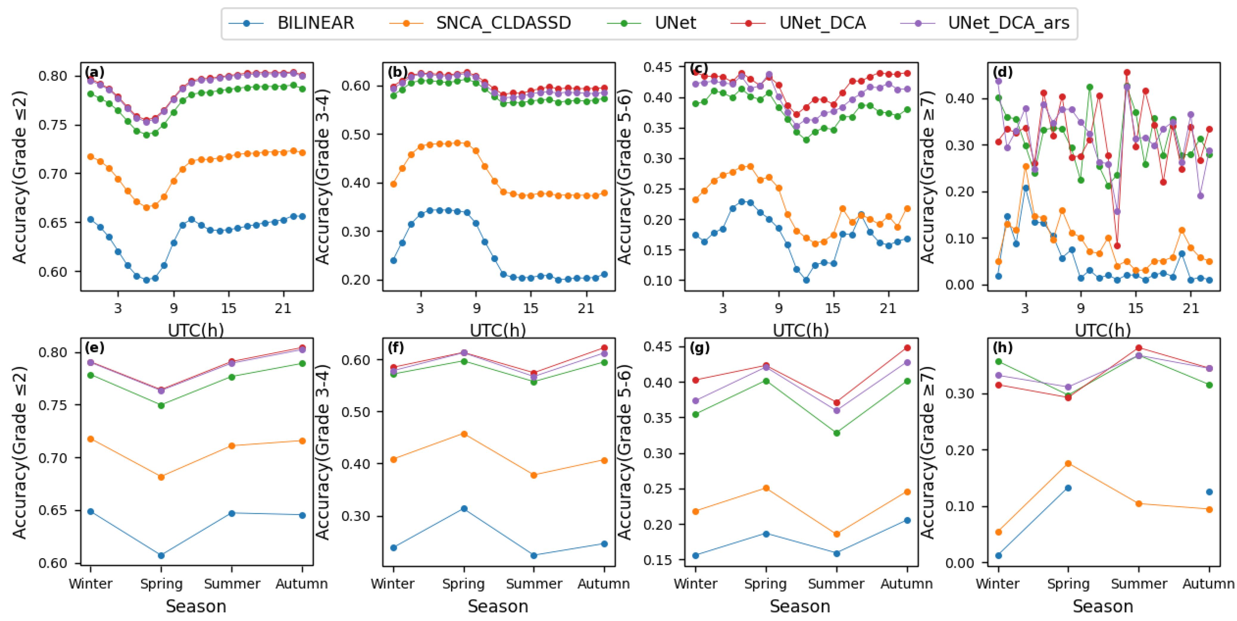
5.4. Assessed by Wind Speed Rating

Table 6. The downscaling results of each method were evaluated according to the accuracy of the wind speed grade; the evaluation index was evaluated with CLDAS3.0 as the Ground Truth; and the optimal index was represented in bold.

Grade	Methods
	BILINEAR	SNCA_CLDASSD	UNET	UNET_DCA	UNET_DCA_ars
≤2	0.635	0.705	0.774	0.788	0.787
3–4	0.259	0.415	0.584	0.603	0.597
5–6	0.184	0.232	0.379	0.420	0.404
≥7	0.167	0.154	0.313	0.322	0.331

presents the wind speed grade accuracy for various downscaling methods calculated using CLDAS3.0 as the Ground Truth. Overall, the accuracy decreases as the grade of wind speed increases. The accuracy for wind speeds equal to or less than grade 2 reaches 0.788, whereas the accuracy for wind speeds equal to or greater than grade 7 only reaches 0.331. UNET_DCA achieves the highest accuracy for wind speeds below grade 7, while UNET_DCA_ars performs best for wind speeds above grade 7.

The first row of Figure 9 presents the diurnal variations in wind speed grade accuracy for various downscaling methods calculated using CLDAS3.0 as the Ground Truth. For the accuracy of wind speeds equal to or less than grade 2 (Figure 9a), the trends of all methods are generally similar, gradually decreasing around 00:00 UTC, reaching a minimum by 06:00, and then gradually increasing, maintaining a relatively stable trend after 10:00. Regarding wind speeds of grades 3 to 4 (Figure 9b), the trends of all methods are also quite similar, starting to rise around 00:00, peaking at 04:00, maintaining the peak until 09:00, then gradually decreasing to a minimum by 12:00, followed by a relatively stable trend. For wind speeds of grades 5 to 6 (Figure 9c), all methods show similar high and low value positions, reaching a peak around 05:00 and a minimum around 12:00. As for wind speeds equal to or greater than grade 7 (Figure 9d), the trends of the methods are not consistent. On the whole, for light wind speeds (equal to or less than Beaufort scale 2), the daytime accuracy is low while the nighttime accuracy is high; for moderate wind speeds (Beaufort scale 3–6), the daytime accuracy is high and the nighttime accuracy is low; for high wind speeds (equal to or greater than Beaufort scale 7), there is no clear pattern. This may be related to the following factors: light wind speed samples mainly occur at night, moderate wind speed samples predominantly appear during the day, and there is a minimal amount of high wind speed samples. The model has learned more from the patterns of larger samples, leading to insufficient learning capacity for the smaller samples. The accuracy for all wind grades is best exhibited by UNET_DCA_ars or UNET_DCA.

The second row of Figure 9 presents the seasonal variations in wind speed grade accuracy for various downscaling methods calculated using CLDAS3.0 as the Ground Truth. For wind speeds equal to or less than grade 2 (Figure 9e), the accuracy is lowest in spring and highest in autumn. Regarding wind speeds of grades 3 to 4 and 5 to 6 (Figure 9f,g), accuracy is poorest in summer and best in spring. For wind speeds equal to or greater than grade 7 (Figure 9h), bilinear interpolation and SNCA_CLDASSD exhibit the lowest accuracy in spring and winter, with the highest accuracy in spring, while the other three UNET architecture models perform the worst in spring and the best in summer.

6. Discussion

The near-surface wind is not only related to the large-scale wind field but also associated with the boundary layer at a finer horizontal scale. Therefore, efficient extraction of features at different scales plays a crucial role in the accuracy of the spatial downscaling of wind fields. To better reconstruct wind fields, this study primarily focuses on how to enhance the learning of relationships between wind fields and terrain at various scales. Numerous scientific experiments have shown that the multi-level feature extraction and skip connections of the UNET architecture can integrate information from different scales. Hence, this research incorporates channel and Spatial Cross-Attention mechanisms into the UNET architecture. Experimental results demonstrate that the UNET_DCA model with Dual Cross-Attention mechanisms achieves the best evaluation metrics. At the same time, when compared with the SNCA-CLDASSD model, which is based on sequentially stacked CNN convolutional modules, the UNET-based model significantly outperforms SNCA-CLDASSD, reconstructing more detailed small-scale wind field features.

The wind field downscaling model established in this paper can be used to backtrack historical data prior to 2008 and generate high-resolution long-term time series products, which is of great significance for enhancing our understanding of wind field dynamics and models. This is mainly reflected in two aspects: Firstly, high-resolution wind field data can more accurately demonstrate the temporal variation trends and regional differences of wind fields, which helps identify the long-term impact of climate change on wind field patterns. Secondly, high-resolution wind field data over a long time series enables researchers to conduct detailed analyses of the regulatory effect of complex terrain on wind fields. Such analyses contribute to the establishment of accurate models of terrain influence, improving the understanding of local climate and weather phenomena. Therefore, improving the accuracy of wind field downscaling is of great importance, and we will continue to delve into this research in the future to further enhance its accuracy.

However, all models experience a decrease in prediction accuracy with higher wind speed grades. The prediction accuracy for wind speeds above grade 7 only reaches a maximum of 33.1%, significantly lower than the accuracy for low wind speeds. One potential reason for this discrepancy may be the scarcity of samples for high wind speeds compared to low wind speeds, leading the models to primarily learn patterns from the more abundant low wind speed samples. Therefore, future research could focus on expanding the training samples for high wind speeds. Another contributing factor to the aforementioned results could be the close relationship between surface winds and upper winds. Typically, when winds are strong in the upper air, they also tend to be strong at the surface. Future steps could involve supplementing additional auxiliary data, such as wind at 850 hPa and 700 hPa levels.

This study focuses on the application of the improved UNET_DCA model based on the UNET architecture in wind field downscaling. By incorporating a Dual Cross-Attention mechanism, the model’s capability for handling complex terrain feature recognition has been effectively enhanced, demonstrating excellent performance. Although satisfactory results have been achieved, the UNET_DCA and the emerging Transformer architectures each have their own strengths in wind field prediction tasks. The advantage of the UNET_DCA model lies in its efficient processing of spatial structural information, particularly the accurate capture of local features, which is crucial for the analysis of terrain effects on wind fields. Furthermore, its lightweight computational characteristics enable rapid iteration and deployment even in resource-constrained environments, making it suitable for handling large-scale wind field datasets. In comparison, the Transformer model is renowned for its powerful global attention mechanism, which can capture long-range dependencies and thus has inherent advantages in understanding large-scale wind flow patterns and overall wind speed distributions. However, the Transformer model’s drawbacks include its higher computational cost and memory requirements, which may become limiting factors when processing high-resolution wind field data. Additionally, the direct application of Transformers to spatial data poses a challenge in terms of their lack of direct capture of local features. Given the unique advantages of the Transformer architecture in handling global dependencies and sequential data, our research team plans to explore its application in wind field downscaling in future work. The focus will be on optimizing the Transformer architecture to maintain a global perspective while effectively utilizing local information, as well as exploring hybrid model designs that combine the strengths of UNET and Transformer with the aim of further improving the accuracy of wind field downscaling while maintaining computational efficiency.

7. Conclusions

To enhance the understanding of the relationship between the wind field and terrain across different scales, this paper introduces a deep learning model, UNET_DCA, based on the UNET architecture. The model incorporates Channel Cross-Attention (CCA) and Spatial Cross-Attention (SCA) mechanisms. Its objective is to achieve the spatial downscaling of near-surface 10 m wind field data from the China Meteorological Administration Land Data Assimilation System (CLDAS) from a coarse scale of 0.0625° to a fine scale of 0.01°, thereby reconstructing high-resolution and high-quality land assimilation products before 2008 and thus filling historical gaps in CLDAS3.0. Through ablation comparison experiments, the following conclusions are drawn:

(1)

The performance of deep learning models significantly surpasses that of the traditional bilinear interpolation method. Models based on the UNET architecture outperform SNCA_CLDASSD, showcasing the UNET’s ability to extract multi-level features and capture richer spatial information in wind field downscaling. UNET models with Cross-Attention mechanisms (CCA and SCA) outperform those without, demonstrating the effectiveness of these mechanisms. UNET_DCA, incorporating both channel and Spatial Cross-Attention mechanisms, outperforms UNET_CCA and UNET_SCA, showing superior performance in RMSE, MAE, and COR metrics. It outperforms BILINEAR by 50.19%, 51.47%, and 33.05%, and outperforms UNET by 6.54%, 8.49%, respectively. Additionally, UNET_DCA_ars, with more auxiliary information, excels in PSNR and SSIM indexes, displaying improvements of 30.21% and 37.07% over BILINEAR and showcasing enhancements of 4.33% and 3.29% over UNET.

(2)

Based on the terrain assessment results, UNET_DCA demonstrates superior performance in RMSE, MAE, and COR across mountain, plateau, basin, and valley regions. On the other hand, UNET_DCA_ars excels in PSNR and SSIM metrics across all terrains and also leads in RMSE, MAE, and COR in plain areas. This suggests that UNET_DCA shows a stronger correlation with actual values, while UNET_DCA_ars excels in preserving the quality and structural similarity of wind field images and capturing finer details in plain regions. At the same time, it can be seen from the comparison of visual images that the downscaling result of the bilinear interpolation method increases the number of grids, making it difficult to reconstruct the corresponding details. In contrast, the deep learning model can reconstruct the spatial details of the wind field, and UNET_DCA_ars can capture more delicate details.

(3)

The results of the time-based evaluation show that all indexes of all methods have the same trend over time in the intraday variation, and all deep learning models also perform poorly in the period of poor bilinear interpolation performance, indicating that data quality determines the upper limit of downscaling results, and the better the data quality, the better the downscaling results. Except for the COR index, the other four indexes were worse in the daytime and better at night. In general, SNCA_CLDASSD performs significantly better than bilinear interpolation in each season, while UNET is significantly better than SNCA_CLDASSD, and UNET_DCA is slightly better than UNET.

(4)

According to wind speed grade, the evaluation results indicate decreasing accuracy with higher wind speeds. UNET_DCA performs best for winds below grade 7, while UNET_DCA_ars excels for winds grade 7 and above. Small wind speed (less than or equal to 2 wind) has low accuracy during the day, high accuracy at night, the lowest accuracy in spring, and the highest accuracy in autumn; moderate wind speed (3~6 wind) has high accuracy during the day, low accuracy at night, the lowest accuracy in summer, and the highest accuracy in spring. For significant wind speeds (grade 7 and above), there are no apparent regular patterns in intra-day and intra-seasonal accuracy changes.

References

1. Han, S.; Shi, C.; Xu, B.; Sun, S.; Zhang, T.; Jiang, L.; Liang, X. Development and evaluation of hourly and kilometer resolution retrospective and real-time surface meteorological blended forcing dataset (SMBFD) in China. J. Meteorol. Res. 2019, 33, 1168–1181. [Google Scholar] [CrossRef]
2. Griggs, D.J.; Noguer, M. Climate change 2001: The scientific basis. In Contribution of Working Group I to the Third Assessment Report of the Intergovernmental Panel on Climate Change; Cambridge University Press: Cambridge, UK, 2002; Volume 57, pp. 267–269. [Google Scholar]
3. Huang, X.; Rhoades, A.M.; Ullrich, P.A.; Zarzycki, C.M. An evaluation of the variable-resolution CESM for modeling California’s climate. J. Adv. Model. Earth Syst. 2016, 8, 345–369. [Google Scholar] [CrossRef]
4. Chen, L.; Liang, X.Z.; DeWitt, D.; Samel, A.N.; Wang, J.X. Simulation of seasonal US precipitation and temperature by the nested CWRF-ECHAM system. Clim. Dyn. 2016, 46, 879–896. [Google Scholar] [CrossRef]
5. Stehlík, J.; Bárdossy, A. Multivariate stochastic downscaling model for generating daily precipitation series based on atmospheric circulation. J. Hydrol. 2002, 256, 120–141. [Google Scholar] [CrossRef]
6. Hertig, E.; Jacobeit, J. Assessments of Mediterranean precipitation changes for the 21st century using statistical downscaling techniques. Int. J. Climatol. J. R. Meteorol. Soc. 2008, 28, 1025–1045. [Google Scholar] [CrossRef]
7. Semenov, M.A. Simulation of extreme weather events by a stochastic weather generator. Clim. Res. 2008, 35, 203–212. [Google Scholar] [CrossRef]
8. Ailliot, P.; Allard, D.; Monbet, V.; Naveau, P. Stochastic weather generators: An overview of weather type models. J. Société Française Stat. 2015, 156, 101–113. [Google Scholar]
9. Kwon, M.; Kwon, H.H.; Han, D. A spatial downscaling of soil moisture from rainfall, temperature, and AMSR2 using a Gaussian-mixture nonstationary hidden Markov model. J. Hydrol. 2018, 564, 1194–1207. [Google Scholar] [CrossRef]
10. Sun, X.; Wang, J.; Zhang, L.; Ji, C.; Zhang, W.; Li, W. Spatial downscaling model combined with the Geographically Weighted Regression and multifractal models for monthly GPM/IMERG precipitation in Hubei Province, China. Atmosphere 2022, 13, 476. [Google Scholar] [CrossRef]
11. Chan, K.C.; Zhou, S.; Xu, X.; Loy, C.C. Basicvsr++: Improving video super-resolution with enhanced propagation and alignment. In Proceedings of the IEEE/CVF Conference on Computer Vision and Pattern Recognition, New Orleans, LA, USA, 18–24 June 2022; pp. 5972–5981. [Google Scholar]
12. Ranade, R.; Liang, Y.; Wang, S.; Bai, D.; Lee, J. 3D Texture Super Resolution via the Rendering Loss. In Proceedings of the ICASSP 2022–2022 IEEE International Conference on Acoustics, Speech and Signal Processing (ICASSP), Virtual, 7–13 May 2022; IEEE: Piscataway, NJ, USA, 2022; pp. 1556–1560. [Google Scholar]
13. Wang, P.; Bayram, B.; Sertel, E. A comprehensive review on deep learning based remote sensing image super-resolution methods. Earth-Sci. Rev. 2022, 232, 104110. [Google Scholar] [CrossRef]
14. Choi, H.; Lee, J.; Yang, J. N-gram in swin transformers for efficient lightweight image super-resolution. In Proceedings of the IEEE/CVF Conference on Computer Vision and Pattern Recognition, Vancouver, BC, Canada, 17–24 June 2023; pp. 2071–2081. [Google Scholar]
15. Leinonen, J.; Nerini, D.; Berne, A. Stochastic super-resolution for downscaling time-evolving atmospheric fields with a generative adversarial network. IEEE Trans. Geosci. Remote Sens. 2020, 59, 7211–7223. [Google Scholar] [CrossRef]
16. Wang, F.; Tian, D.; Lowe, L.; Kalin, L.; Lehrter, J. Deep learning for daily precipitation and temperature downscaling. Water Resour. Res. 2021, 57, e2020WR029308. [Google Scholar] [CrossRef]
17. Harris, L.; McRae, A.T.; Chantry, M.; Dueben, P.D.; Palmer, T.N. A generative deep learning approach to stochastic downscaling of precipitation forecasts. J. Adv. Model. Earth Syst. 2022, 14, e2022MS003120. [Google Scholar] [CrossRef] [PubMed]
18. Gerges, F.; Boufadel, M.C.; Bou-Zeid, E.; Nassif, H.; Wang, J.T.L. A Novel Deep Learning Approach to the Statistical Downscaling of Temperatures for Monitoring Climate Change. In Proceedings of the 2022 The 6th International Conference on Machine Learning and Soft Computing, Haikou, China, 15–17 January 2022; pp. 1–7. [Google Scholar]
19. Vandal, T.; Kodra, E.; Ganguly, S.; Michaelis, A.; Nemani, R.; Ganguly, A.R. Deepsd: Generating high resolution climate change projections through single image super-resolution. In Proceedings of the 23rd ACM SIGKDD International Conference on Knowledge Discovery and Data Mining, Halifax, NS, Canada, 13–17 August 2017; pp. 1663–1672. [Google Scholar]
20. Mao, Z. Spatial Downscaling of Meteorological Data Based on Deep Learning Image Super-Resolution. Master’s Thesis, Wuhan University, Wuhan, China, 2019. [Google Scholar]
21. Tie, R.; Shi, C.; Wan, G.; Hu, X.; Kang, L.; Ge, L. CLDASSD: Reconstructing fine textures of the temperature field using super-resolution technology. Adv. Atmos. Sci. 2022, 39, 117–130. [Google Scholar] [CrossRef]
22. Tie, R.; Shi, C.; Wan, G.; Kang, L.; Ge, L. To Accurately and Lightly Downscale the Temperature Field by Deep Learning. Ournal Atmos. Ocean. Technol. 2022, 39, 479–490. [Google Scholar] [CrossRef]
23. Shen, Z.; Shi, C.; Shen, R.; Tie, R.; Ge, L. Spatial Downscaling of Near-Surface Air Temperature Based on Deep Learning Cross-Attention Mechanism. Remote Sens. 2023, 15, 5084. [Google Scholar] [CrossRef]
24. Höhlein, K.; Kern, M.; Hewson, T.; Westermann, R. A comparative study of convolutional neural network models for wind field downscaling. Meteorol. Appl. 2020, 27, e1961. [Google Scholar] [CrossRef]
25. Dupuy, F.; Durand, P.; Hedde, T. Downscaling of surface wind forecasts using convolutional neural networks. Nonlinear Process. Geophys. 2023, 30, 553–570. [Google Scholar] [CrossRef]
26. Lin, H.; Tang, J.; Wang, S.; Wang, S.; Dong, G. Deep learning downscaled high-resolution daily near surface meteorological datasets over east asia. Sci. Data 2023, 10, 890. [Google Scholar] [CrossRef]
27. Gorkem, C.A.; Prasoon, M.; Emrah, C. Dual Cross-Attention for medical image segmentation. Eng. Appl. Artif. Intell. 2023, 126, 107139. [Google Scholar]
28. Zhou, Y.; Huo, C.; Zhu, J.; Huo, L.; Pan, C. DCAT: Dual Cross-Attention-Based Transformer for Change Detection. Comput. Biol. Med. 2023, 15, 2395. [Google Scholar] [CrossRef]
29. Fu, Z.; Li, J.; Hua, Z. DEAU-Net: Attention networks based on dual encoder for Medical Image Segmentation. Comput. Biol. Med. 2022, 150, 106197. [Google Scholar] [CrossRef] [PubMed]
30. Han, S.; Liu, B.; Shi, C.; Liu, Y.; Qiu, M.; Sun, S. Evaluation of CLDAS and GLDAS datasets for Near-surface Air Temperature over major land areas of China. Sustainability 2020, 12, 4311. [Google Scholar] [CrossRef]
31. Reuter, H.I.; Nelson, A.; Jarvis, A. An evaluation of void-filling interpolation methods for SRTM data. Int. J. Geogr. Inf. Sci. 2007, 21, 983–1008. [Google Scholar] [CrossRef]
32. QX/T 118-2020; Meteorological Observation Data Quality Control. Chinese Industry Standard: Beijing, China, 2020.
33. Olaf, R.; Philipp, F.; Thomas, B. U-net: Convolutional networks for biomedical images egmentation. In Proceedings of the Medical Image Computing and Computer-Assisted Intervention–MICCAI 2015: 18th International Conference, Munich, Germany, 5–9 October 2015; pp. 234–241. [Google Scholar]
34. Jha, D.; Riegler, M.A.; Johansen, D.; Halvorsen, P.; Johansen, H.D. Doubleu-net: A deep convolutional neural network for medical image segmen-tation. In Proceedings of the 2020 IEEE 33rd International Symposium on Computer-Based Medical Systems (CBMS), Rochester, MN, USA, 28–30 July 2020; pp. 558–564. [Google Scholar]
35. Bao, K.; Zhang, X.; Peng, W.; Yao, W. Deep learning method for super-resolution reconstruction of the spatio-temporal flow field. Adv. Aerodyn. 2023, 5, 19. [Google Scholar] [CrossRef]
36. Xiao, Y.; Zhang, J.; Chen, W.; Wang, Y.; You, J.; Wang, Q. SR-DeblurUGAN: An End-to-End Super-Resolution and Deblurring Model with High Performance. Drones 2022, 6, 162. [Google Scholar] [CrossRef]
37. Fan, Z.; Dan, T.; Liu, B.; Sheng, X.; Yu, H.; Cai, H. SGUNet: Style-guided UNet for adversely conditioned fundus image super-resolution. Neurocomputing 2021, 465, 238–247. [Google Scholar] [CrossRef]
38. Mela, C.A.; Liu, Y. Application of convolutional neural networks towards nuclei segmentation in localization-based super-resolution fluorescence microscopy images. BMC Bioinform. 2021, 1, 325. [Google Scholar] [CrossRef]
39. Chen, F.; Manning, K.W.; LeMone, M.A.; Trier, S.B.; Alfieri, J.G.; Roberts, R.; Tewari, M.; Niyogi, D.; Horst, T.W.; Oncley, S.P.; et al. Description and evaluation of the characteristics of the NCAR high-resolution land data assimilation system. J. Appl. Meteorol. Climatol. 2007, 46, 694–713. [Google Scholar] [CrossRef]
Figure 1. The figure on the left (a) illustrates the spatial arrangement of national meteorological stations (marked by red stars) and regional meteorological stations (depicted as green dots) within the study area. On the right (b), the figure displays the distribution of ground elevation across the research area, segmented into 49 distinct zones. Table 1 provides a breakdown of the terrain types corresponding to each of these areas.
Remotesensing 16 01867 g001
Figure 2. The first column displays statistical histograms for Mean Absolute Error (MAE) and Correlation (COR) of regional site data; the second column shows the violin plots of MAE and COR for regional site data before data cleansing; the third column presents the violin plots of MAE and COR for regional site data after data cleansing.
Remotesensing 16 01867 g002
Figure 3. The architecture diagram of the UNET_DCA network model.
Remotesensing 16 01867 g003
Figure 4. The structure diagram of the Dual Interlaced Attention Module (DCA) consists of two modules: (a) the Channel Interlaced Attention Module and (b) the Spatial Interlaced Attention Module.
Remotesensing 16 01867 g004
Figure 5. Box plots of wind speed RMSE, MAE, and COR metrics based on station data as the Ground Truth for the downscaling results of each method.
Remotesensing 16 01867 g005
Figure 6. Visual comparison of downscaling results of various methods at 12:00 UTC on 24 April 2019.
Remotesensing 16 01867 g006
Figure 7. Daily variations of RMSE, MAE, COR, PSNR, and SSIM between downscaling wind speed results of each method and CLDAS3.0.
Remotesensing 16 01867 g007
Figure 8. Seasonal variations of RMSE, MAE, COR, PSNR, and SSIM between each method’s downscaling wind speed results and CLDAS3.0.
Remotesensing 16 01867 g008
Figure 9. The first row presents diagrams illustrating the diurnal variation in the accuracy of wind speed grade calculations derived from each downscaling method, with (ad) corresponding to the four wind speed categories, respectively. The second row depicts the seasonal variation in the correctness of wind speed grade estimations achieved by the various downscaling techniques, where (eh) respectively match the four distinct wind speed classes.
Remotesensing 16 01867 g009