An Optical Detection Model for Stratospheric Airships

Abstract

This study proposes a numerical model to simulate the thermal characteristics of stratospheric airships (SA). This model introduces a simple yet accurate method for the selection of the optical bands for target detection based on multispectral features. The key to this model is the selection of the spectral bands in which a significant radiation difference exists between the target and its surrounding background. Using the signal-to-noise ratio (SNR), detection probability, and false alarm rate as model evaluation metrics, and based on the analysis of the radiation differences between the target and atmospheric background, it is found that there are two narrow bands possible for SA detection: one with a central wavelength of 8.83 µm and a bandwidth of 0.35 µm and the other with a central wavelength of 11.51 µm and a bandwidth of 0.34 µm. Further numerical simulations and theoretical analyses under varying space environments demonstrate that considerable detection potential can be achieved; thus, the presented optical detection model is useful for the night detection of SA targets.

1. Introduction

Stratospheric airships are generally large airships flying in the lower regions of the stratosphere within weak wind zones, using their own propulsion to overcome the wind resistance and achieve prolonged stationary positioning or cruising [1,2]. These airships are versatile and cost-effective and find application in diverse fields, such as ground surveillance [3], Earth observation [4], intelligence and reconnaissance [5], missile defense [6], aviation transportation [7], environmental monitoring [8], planetary exploration [9], and telecommunication relays [10]. In the military domain, comparatively inexpensive communication platforms offer excellent long-term surveillance capabilities. In the general civilian domain, they can be employed to observe changes in the Earth’s environment, collect meteorological data, and conduct environmental surveillance or monitoring in predetermined areas [11]. Over the past few decades, extensive studies have been conducted to model and simulate the thermal characteristics of stratospheric airships. Kreith and Kreider [12,13] established a simple yet excellent numerical model to simulate the average temperature of the balloon envelope and lifting gas, which marked the starting point for subsequent research. Carlson and Horn [14] incorporated the influence of water vapor based on Kreith’s model and developed a new computer model to predict the trajectory and thermal behavior of high-altitude balloons. Louchev [15] developed a steady-state model for airships and hot air balloon shells by considering the convective heat transfer on the external surface of the shell for forced and natural convection to compute the temperature fields under various conditions. Farley [16] created new, user-friendly software to simulate the vertical and horizontal motion of high-altitude balloons, which is also applicable for the simulation of balloon flight in other atmospheres on different planets. Xia et al. [17] developed a three-dimensional transient model to predict diurnal variations in skin and lifting gas temperatures under float conditions. Liu et al. [18] proposed a numerical model to investigate the thermal and dynamic properties of scientific balloons during ascent and floating. Based on certain assumptions and simplifications, Shi et al. [19] developed a thermal model to describe the heat transfer behavior of stratospheric airships. It was observed that factors such as the airship velocity, air filling, and air venting significantly affected the thermal performance. K. Stefan [20] established a steady-state model for airships, suggesting a temperature difference of approximately 51 K between the helium gas temperatures during the day and night under clear sky conditions. Franco et al. [21] developed a three-dimensional thermal model for high-altitude balloons, considering the influences of solar radiation, reflected radiation, and the Earth’s infrared radiation while not accounting for convective heat transfer.

Research on target detection using such platforms has significant value in aviation, aerospace, and related sectors. Research on target detection has become a primary application in the field of national defense and security, and it has played an indispensable role in national security. The ability to acquire information about space targets to some extent represents a country’s core strength in modern military warfare [22]. The detection of targets largely depends on several factors: the radiation characteristics of the targets and the surrounding background, as well as the contrast between them [23]. Target detection is often influenced by the atmospheric conditions, and the radiation characteristics of the target and the background reaching the observer are subjected to atmospheric transmission effects, leading to radiation attenuation. Atmospheric or solar radiation simultaneously contributes to the generation of background radiation. In instances where the background radiation or atmospheric attenuation is strong, the target signal can be completely masked, making detection impossible [24]. With the rapid advancement of spectral technology, its inherent advantages, such as a high resolution and suitability for quantitative analysis, have led to widespread application in target detection. However, the selection of detection bands is crucial when using spectral technology for target detection. Zong et al. [25] conducted research on the infrared radiation characteristics of stealth aircraft plumes, identifying the spectral bands where the plume radiation energy is concentrated under various common stealth measures. Gao et al. [26] studied the infrared radiation characteristics of aircraft plumes and developed a quantitative analysis model. Karlholm et al. [27] focused on selecting appropriate filters to suppress background clutter and achieve high SNRs. Ni et al. [28] proposed a method to enhance the detection capabilities of stealth aircraft by selecting the optimal spectrum from a spectral set based on the maximum SNR, with the aim of highlighting the detection of aircraft targets. Liu et al. [29] proposed a concise spectral band selection method for precise target detection using significantly reduced infrared radiation from the multispectral features of a stealth aircraft. Wang et al. [30] introduced a two-step band selection method based on target detection that can improve the target detection effectiveness while reducing the data dimensionality. Lin et al. [31] designed a unit energy spectral detection system to objectively analyze selected detection bands for stealth aircraft detection. The aforementioned research results originate from the radiation characteristics of the targets and propose feasible methods for spectral target detection. However, these studies lack analysis from a systemic perspective and have limited involvement in the detection of stratospheric airships.

This study conducted optical detection research from a systemic perspective by modeling and simulating the entire system for stratospheric airship target detection. This included a calculation model for the stratospheric airship thermal characteristics, an atmospheric background radiation model, and a mathematical model of the entire detection system. This study comprehensively considered the influence of the target background radiation characteristics and detection instrument parameters. The SNR, detection probability, and false alarm rate were used as criteria for band selection, making the research methodology more systematic. Using the South China Sea region as an example, the radiation characteristics of stratospheric airships and atmospheric backgrounds under different sea conditions were analyzed. This analysis led to the proposition of a method for the selection of detection bands.

2. Calculation Model

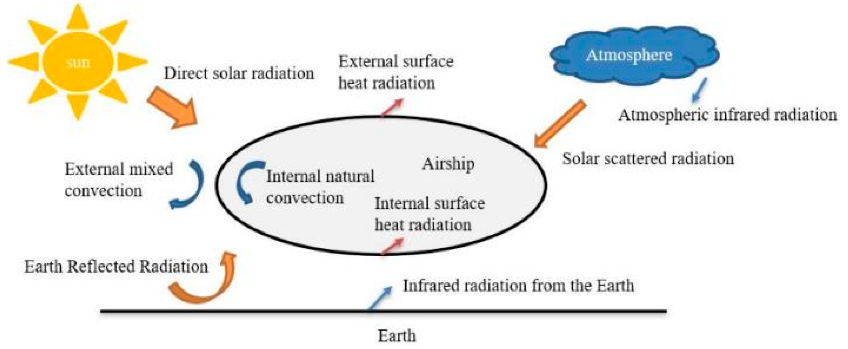
2.1. Modeling of Thermal Characteristics of Stratospheric Airships

Figure 1 illustrates the thermodynamic environment in which a stratospheric airship operates during flight. Externally, it is influenced by solar radiation, atmospheric infrared radiation, the Earth’s infrared radiation, and external convection. Internally, it is affected by natural convection and infrared radiation between the internal surfaces. The thermodynamic environment in which they operate is complex.

This study uses a three-dimensional model that partitions the airship skin into several units and makes the following assumptions:

• The skin thickness is negligible, thus neglecting thermal conduction in the direction of the skin unit thickness and between adjacent units;
• The surface temperatures of the units are uniform and similar to those of the surrounding gas;
• The solar radiation incident on the unit surfaces is uniform, with uniform absorption characteristics for solar radiation;
• The skin is opaque, which prevents solar radiation from passing through.

Considering the aforementioned assumptions, the transient temperature distribution on the skin can be expressed as

$$m_i{c}_s\frac{d{T}_i}{d\tau }=Q_{idn}+Q_{id}+Q_{ie}-Q_{iIR,atm}-Q_{iIR,e}-Q_{ico}-Q_{ici}-Q_{ir}$$

(1)

where $m_i$ is the mass of the unit in kg, $c_s$ is the specific heat of the skin material in J/(kg·K), $T_i$ is the temperature of the skin in K, $Q_{idn}$ is the direct solar radiation flux in W, $Q_{id}$ is the diffuse solar radiation flux in W, $Q_{ie}$ is the reflected Earth radiation flux in W, $Q_{iIR,atm}$ is the atmospheric infrared radiation flux in W, $Q_{iIR,e}$ is the Earth infrared radiation flux in W, $Q_{ico}$ is the external surface maximum convective heat transfer flux in W, $Q_{ici}$ is the internal surface natural convective heat transfer flux in W, and $Q_{ir}$ is the thermal radiation flux between units in W.

2.2. Signal Analysis of Airship Targets

Assuming that the spectral radiance intensity of the target is $I(\lambda )$, the spectral irradiance at the entrance pupil of the camera owing to the target is $H(\lambda )$:

$$H(\lambda )={\tau }_a(\lambda )\frac{I(\lambda )}{L^2}$$

(2)

If the number of imaging elements on the focal plane formed by the target is $n$, then the average spectral radiative flux ${\Phi }_t(\lambda )$ of the target radiation entering the camera aperture and reaching the element is

$${\Phi }_t(\lambda )={\tau }_f(\lambda ){\tau }_a(\lambda )S_D\frac{I(\lambda )}{n\cdot L^2}$$

(3)

$$L=(H-h_0)/\cos \theta$$

(4)

where ${\tau }_a\left(\lambda \right)$ is the atmospheric spectral transmittance from the target to the observation point, $L$ is the observation distance, $\theta$ is the observation angle, $h_0$ is the flight altitude of the target, $H$ is the altitude of the observation point, ${\tau }_f\left(\lambda \right)$ is the spectral transmittance of the optical system, $S_D$ is the entrance pupil area, and $n$ is the number of ageing elements in the image plane of the target.

The unobstructed part, as shown in Figure 2, was filled with the radiation induced by the atmospheric background. The spectral radiative flux ${\Phi }_{bg\_t}(\lambda )$ caused by this portion is expressed as follows:

$${\Phi }_{bg\_t}(\lambda )=L_{bg}(\lambda ){\tau }_f(\lambda )(1-\frac{S_t}{S_s})S_D\Omega =L_{bg}(\lambda ){\tau }_f(\lambda )(1-\frac{S_t}{n\cdot S_d})\cdot FF\cdot \frac{d^2}{f^2}\cdot \frac{\pi D^2}{4}$$

(5)

$$S_t=A_t\cdot {(\frac{f}{L})}^2$$

(6)

$$S_S=n\cdot d^2$$

(7)

where $S_t$ is the area size of the target imaged on the focal plane; $A_t$ is the area of the target; $S_s$ is the total area of the imaged elements on the focal plane; $S_d$ is the area of a single pixel on the focal plane; $L_{bg}\left(\lambda \right)$ is the atmospheric background spectral radiance; $S_D$ is the entrance pupil area; $\Omega$ is the instantaneous field of view solid angle; $d$ is the distance to the center of the element; $f$ is the focal length; $FF$ is the fill factor; and $D$ is the system optical aperture.

The spectral radiative flux induced by the atmosphere from the target position to the observation point is represented by ${\Phi }_{fk}\left(\lambda \right)$.

$${\Phi }_{fk}(\lambda )=L_{bg(h_0-H)}(\lambda ){\tau }_f(\lambda )\frac{S_t}{n\cdot S_d}{S}_D\Omega$$

(8)

where $L_{bg(h_0-H)}(\lambda )$ is the atmospheric spectral radiance from the target position to the observation point.

The radiative flux ${\Phi }_{p\_t}(\Delta \lambda )$ of the target in the spectral band ${\lambda }_1~{\lambda }_2$ within the imaging element is

$${\Phi }_{p\_t}(\Delta \lambda )={\displaystyle {\int }_{{\lambda }_1}^{{\lambda }_2}{\Phi }_{p\_t}(\lambda )d\lambda ={\Phi }_t(\Delta \lambda )}+{\Phi }_{bg\_t}(\Delta \lambda )+{\Phi }_{fk}(\Delta \lambda )$$

(9)

The number of signal electrons $N_{p\_t}(\Delta \lambda )$ generated by the imaging element containing the target is

$$N_{p\_t}(\Delta \lambda )=\eta \cdot \frac{{\Phi }_{p\_t}(\Delta \lambda )\cdot T_{\mathrm{int}}\cdot \overline{\lambda }}{h\cdot c}$$

(10)

where $\overline{\lambda }$ is the central wavelength, $\eta$ is the quantum efficiency, $h$ is Planck’s constant, $c$ is the speed of light, $\lambda$ is the wavelength, and $T_{\mathrm{int}}$ is the integration time.

2.3. Atmospheric Background Signal Analysis

The radiation signal from the upper atmospheric layer was observed when the system imaged the background atmosphere. The average radiative flux ${\Phi }_{bg}\left(\lambda \right)$ introduced by the atmospheric background within the instantaneous field of view (on a single pixel) is

$${\Phi }_{bg}\left(\lambda \right)=L_{bg}\left(\lambda \right){\tau }_f\left(\lambda \right)S_D\Omega$$

(11)

The average radiative flux ${\Phi }_{bg}\left(\lambda \right)$ of the atmospheric background on a single detection element within the ${\lambda }_1~{\lambda }_2$ band.

$${\Phi }_{bg}(\Delta \lambda )={\displaystyle \underset{{\lambda }_1}{\overset{{\lambda }_2}{\int }}{L}_{bg}(\lambda )}{\tau }_f(\lambda )S_D\Omega d\lambda$$

(12)

The number of electrons $N_{bg}\left(\Delta \lambda \right)$ generated by the atmospheric background on a single pixel.

$$N_{bg}(\Delta \lambda )=\eta \cdot \frac{{\Phi }_{bg}(\Delta \lambda )\cdot T_{\mathrm{int}}\cdot ({\lambda }_1+{\lambda }_2)}{2\cdot h\cdot c}$$

(13)

2.4. Signal-to-Noise Ratio Model

The SNR is defined as the ratio of the signal value to the noise value. The expression for the number of signal electrons $N_S\left(\Delta \lambda \right)$ in the band ${\lambda }_1~{\lambda }_2$ is

$$N_S\left(\Delta \lambda \right)=N_{p\_t}\left(\Delta \lambda \right)-N_{bg}\left(\Delta \lambda \right)$$

(14)

The expression for the noise electron count is ${\sigma }_n\left(\Delta \lambda \right)$:

$${\sigma }_n(\Delta \lambda )=\sqrt{{\sigma }_{\det }^2(\Delta \lambda )+{\sigma }_{sp}^2+{\sigma }_q^2+{\sigma }_{out}^2}$$

(15)

where ${\sigma }_{\det }\left(\Delta \lambda \right)$ is the detector noise, ${\sigma }_{sp}$ is the conditioning circuit noise, ${\sigma }_q$ is the quantization noise, and ${\sigma }_{out}$ is the readout noise.

The detector noise is related to the detector element current, which is proportional to the incident radiation flux on the detector element. This relationship can be expressed as

$${\sigma }_{\det }(\Delta \lambda )=\sqrt{\eta \frac{\Phi \left(\Delta \lambda \right)\cdot T_{\mathrm{int}}\cdot \overline{\lambda }}{2\cdot h\cdot c}}$$

(16)

where $\Phi \left(\Delta \lambda \right)$ is the incident radiation flux on the detector element:

$$\Phi \left(\Delta \lambda \right)={\Phi }_{p\_t}\left(\Delta \lambda \right)-{\Phi }_{bg}\left(\Delta \lambda \right)$$

(17)

If the equivalent input noise voltage of the conditioning circuit is $V_{n,sp}$, the detector’s integration capacitance is $C_{\mathrm{int}}$, and the electronic charge is $q$, then the equivalent noise electronic charge at the terminal of the conditioning circuit ${\sigma }_{sp}$ is

$${\sigma }_{sp}=\frac{C_{\mathrm{int}}·V_{n.sp}}{q}$$

(18)

If the number of quantization bits for A/D conversion is $b_q$ and the full well charge of the detector is $Q_{well}$, then the quantization noise ${\sigma }_q$ is

$${\sigma }_q=\frac{Q_{well}}{\sqrt{12}·2^{b_q}·q}$$

(19)

The number of electrons corresponding to the readout circuit noise is the time noise electrons measured under low-exposure conditions.

The expression for $SNR\left(\Delta \lambda \right)$ is

$$SNR(\Delta \lambda )=\frac{N_S(\Delta \lambda )}{{\sigma }_n(\Delta \lambda )}$$

(20)

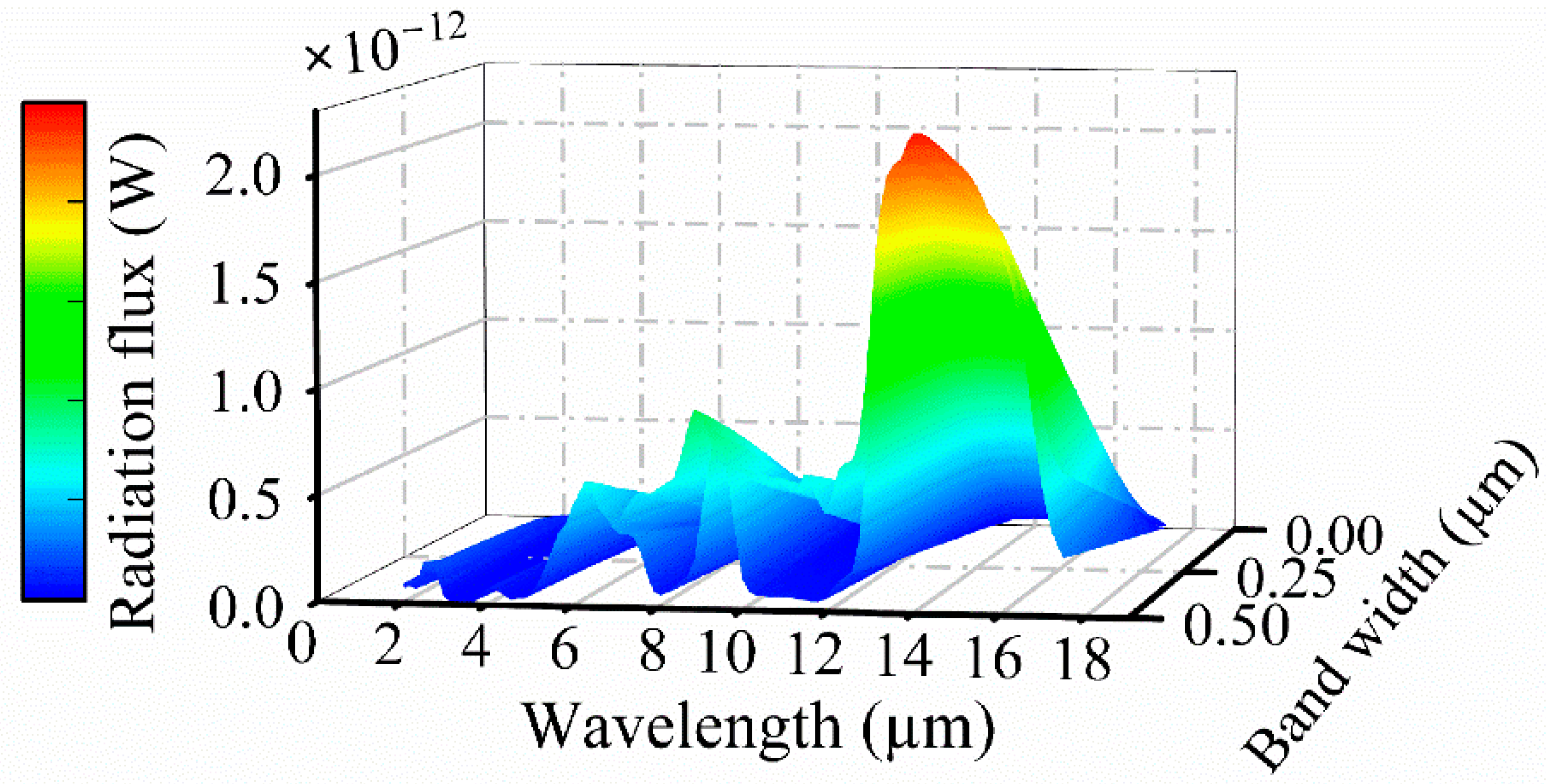
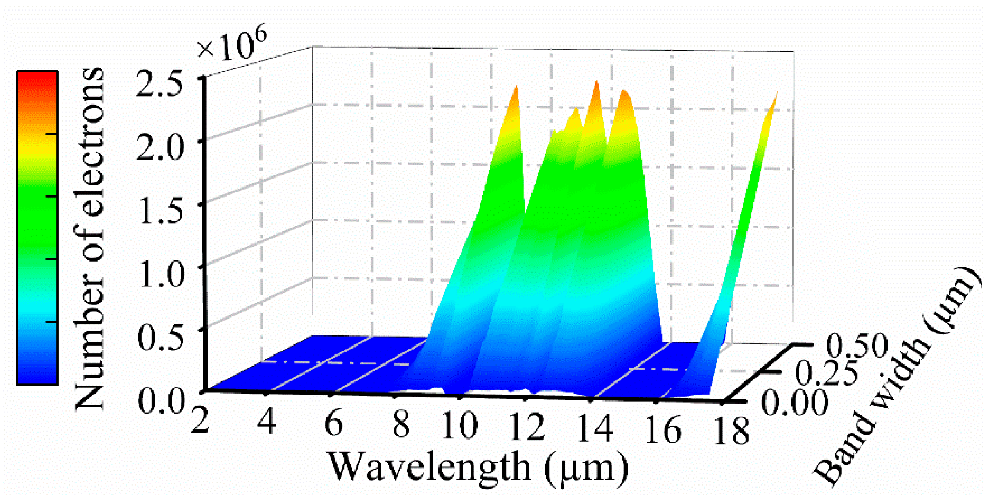
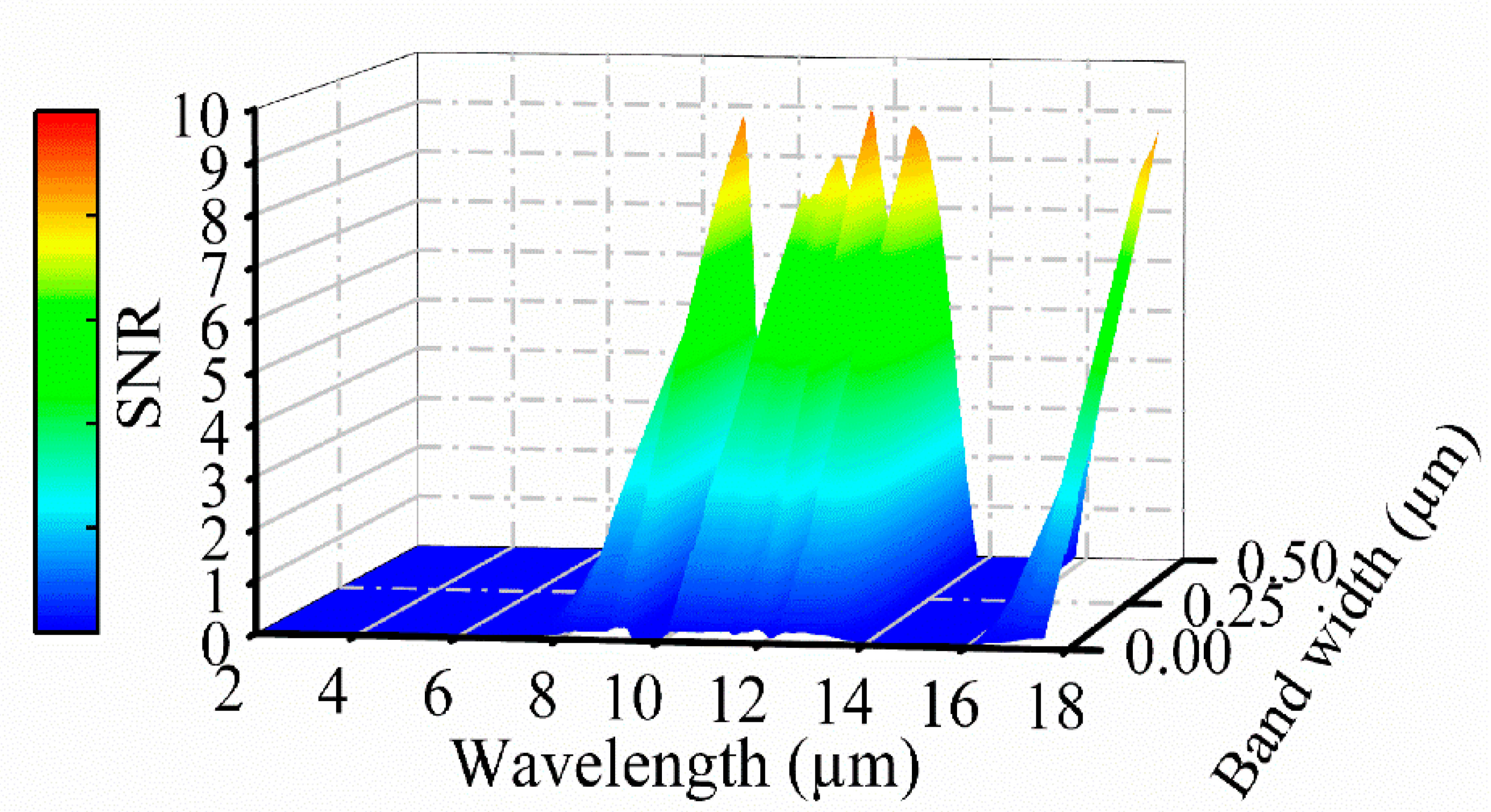
3. Band Selection for Multispectral Detection

3.1. Analysis of Performance Evaluation Indicators for Detection Systems

In target detection systems, statistical detection methods are commonly used to ascertain the presence of a target. Target detection aims to determine whether a target exists in the acquired images and is typically assessed using the detection probability and false alarm rate. The detection probability is the probability of detecting a true target when it is present in the background, whereas the false alarm rate is the probability of detecting a target when it is absent from the background.

Assume two hypothesis models in the background, one with a target and the other without a target—namely, a dual-hypothesis testing model:

$$P_1:X_{ij}=S_{ij}+N_{ij}+C_{ij}$$

(21)

$$P_0:X_{ij}=N_{ij}+C_{ij}$$

(22)

$$I_{ij}=N_{ij}+C_{ij}$$

(23)

where $P_0$ and $P_1$ are two different background clutter scenarios: one without a target and the other with a target, respectively. $X_{ij}$ is the pixel value formed by the focal plane imaging; $S_{ij}$ is the incremental pixel value brought by the target signal; $N_{ij}$ is the incremental pixel value caused by system noise; $C_{ij}$ is the incremental pixel value brought by the background clutter after system imaging; $I_{ij}$ is the system interference signal value.

We assume that $N_{ij}$ and $C_{ij}$ both follow a Gaussian distribution and are mutually independent, where ${\sigma }_n^2$ is the variance of $N_{ij}$, and ${\sigma }_c^2$ is the variance of $C_{ij}$. According to the relevant mathematical theory of probability, the probability density functions of $X_{ij}$ under the two scenarios of $P_0$ and $P_1$ are as follows.

$$p(X_{ij}|P_1)=\frac{1}{\sqrt{2\pi {\sigma }_I}}{e}^{\left[-\frac{{\left(X_{ij}-S_{ij}\right)}^2}{2{\sigma }_I^2}\right]}$$

(24)

$$p(X_{ij}|P_0)=\frac{1}{\sqrt{2\pi {\sigma }_I}}{e}^{\left[-\frac{{\left(X_{ij}\right)}^2}{2{\sigma }_I^2}\right]}$$

(25)

$${\sigma }_I^2={\sigma }_n^2+{\sigma }_c^2$$

(26)

where ${\sigma }_I$ is the standard deviation of the system interference signal; $p\left(X_{ij}|P_1\right)$ and $p\left(X_{ij}|P_0\right)$ are the probability density functions when the target is present and absent, respectively. If a threshold detection algorithm is employed (with a detection threshold of $S_0$) for target detection, the detection probability $P_d$ for the target is the integral of $p\left(X_{ij}|P_1\right)$ when $X_{ij}>S_0$:

$$P_d={\displaystyle \underset{T_0}{\overset{\infty }{\int }}p(X_{ij}|P_1)d{X}_{ij}=\frac{1}{2}[1+erf(\frac{S-S_0}{\sqrt{2}{\sigma }_I})]}$$

(27)

The false alarm rate of target detection $P_f$ is the integral over $p\left(X_{ij}|P_0\right)$ when $X_{ij}>S_0$:

$$P_f={\displaystyle \underset{T_0}{\overset{\infty }{\int }}p(X_{ij}|P_0)d{X}_{ij}=\frac{1}{2}[1-erf(\frac{S_0}{\sqrt{2}{\sigma }_I})]}$$

(28)

where $erf\left(x\right)$ is the error function of the independent variable $x$, defined as

$$erf(x)=\frac{2}{\sqrt{\pi }}{\displaystyle \underset{0}{\overset{x}{\int }}{e}^{-{\eta }^2}}d\eta$$

(29)

Defining the signal-to-interference ratio $SIR$ of the system,

$$SIR=\frac{S}{{\sigma }_I}$$

(30)

where $S$ is the target signal.

Substituting Equations (29) and (30) into Equations (27) and (28) yields the following expression.

$$P_d=\frac{1}{2}[1+erf(\frac{SIR-TIR}{\sqrt{2}})]$$

(31)

$$P_f=\frac{1}{2}[1-erf(\frac{TIR}{\sqrt{2}})]$$

(32)

where $TIR$ is the signal-to-interference-ratio threshold selected during the target detection process.

$$TIR=\frac{S_0}{{\sigma }_I}$$

(33)

where $S_0$ is the detection threshold.

A high-performance target search and detection system requires a high target detection probability and the smallest possible false alarm rate to effectively improve the target detection probability in the background, without mistakenly identifying other sources of interference. The only way to achieve this is to elevate the signal-to-interference ratio threshold appropriately and maximize the SNR of the system.

As shown in Figure 3, for the detection of the same target in the same scene with the same threshold—that is, the same false alarm rate—a higher signal-to-interference ratio (SIR) corresponds to a higher detection probability. When maintaining a constant SIR for target detection, reducing the false alarm rate inevitably decreases the detection probability. Therefore, in such a scenario, a higher demand can only be placed on the SIR.

$$SIR=\frac{1}{\sqrt{\frac{1}{SN{R}^2}+\frac{1}{SC{R}^2}}}$$

(34)

where $SNR=\frac{S}{{\sigma }_n}$ is the system’s SNR, and $SCR=\frac{S}{{\sigma }_c}$ is the system’s signal-to-clutter ratio.

To achieve target detection, the system typically requires a detection probability of $P_d>95\%$ and a false alarm rate of $P_f<0.001\%$. The SNR threshold of the system was computed using $SN{R}_{th}=6$.

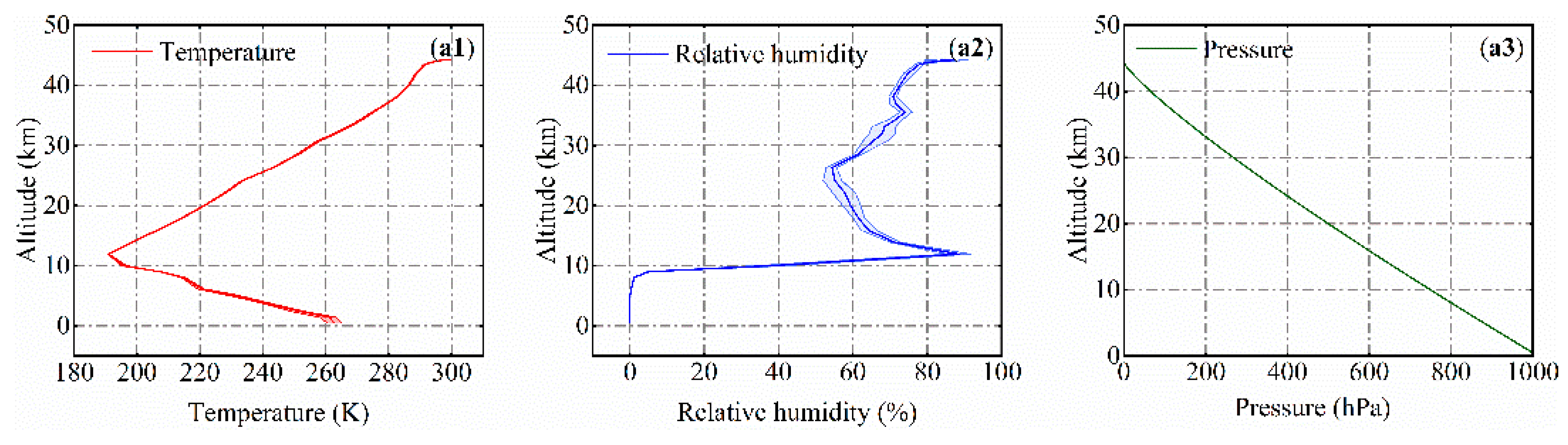
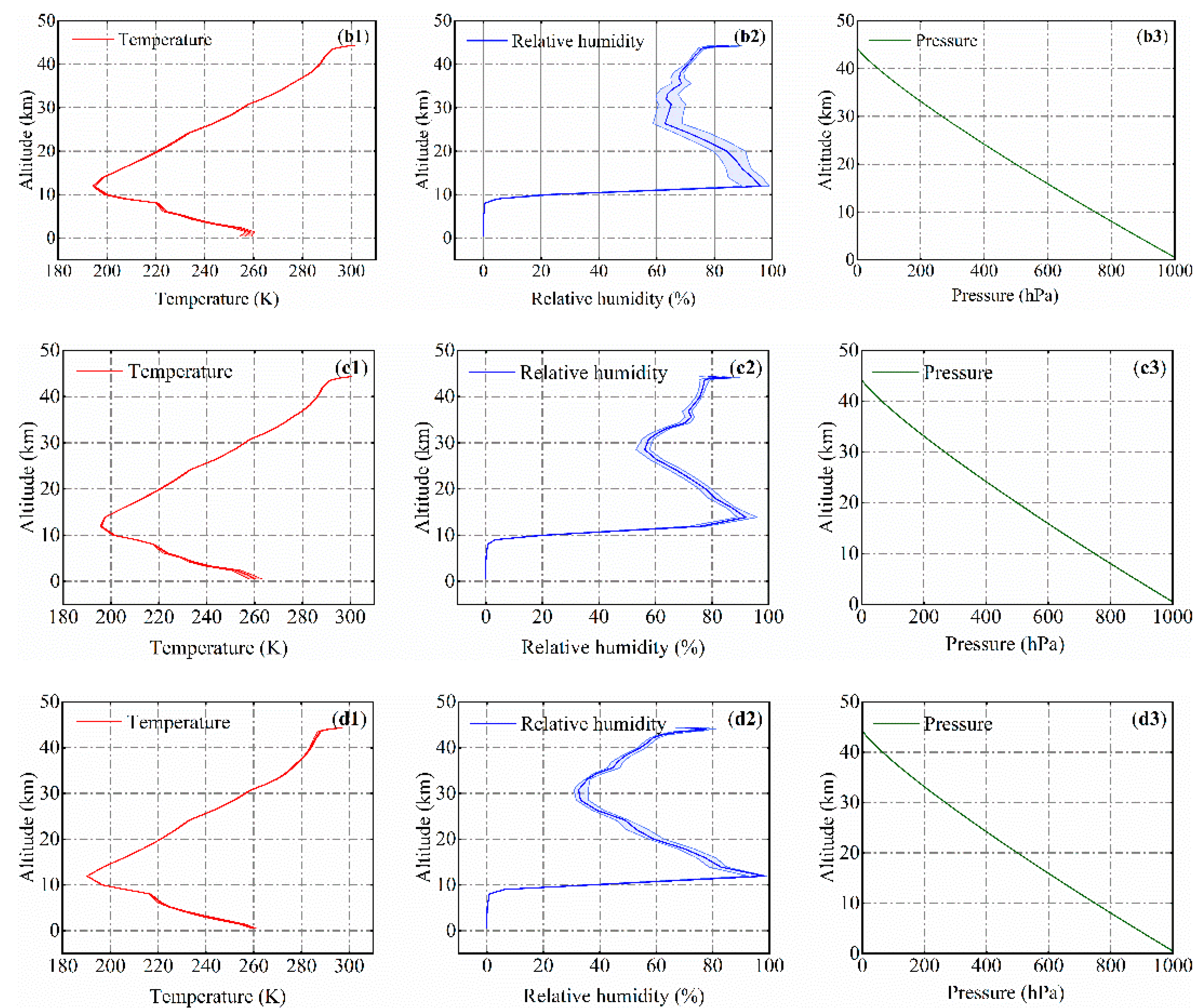
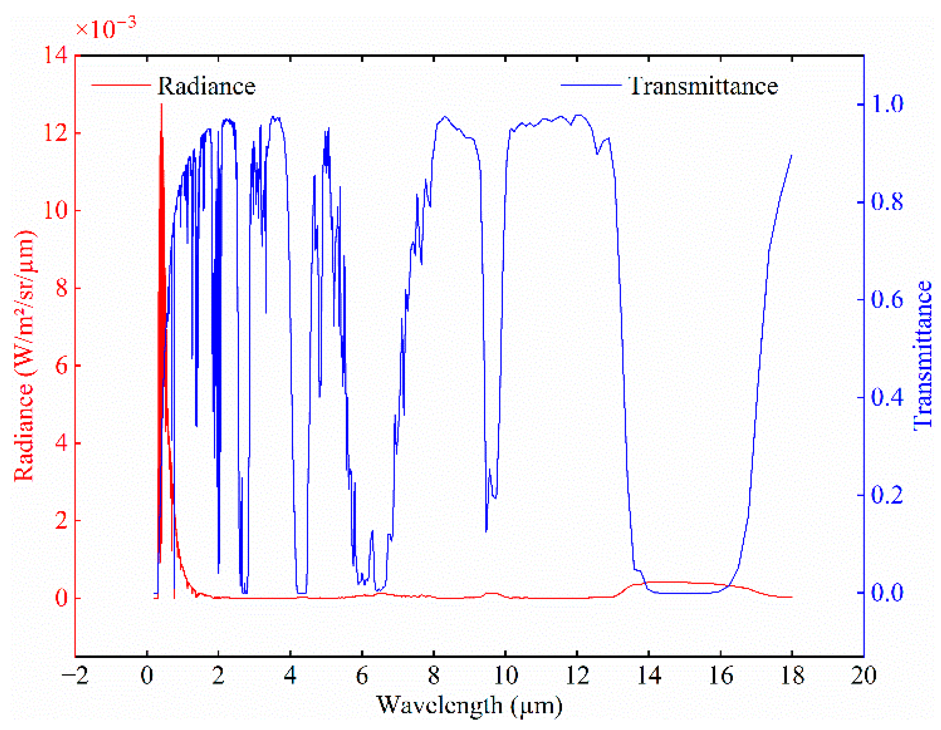
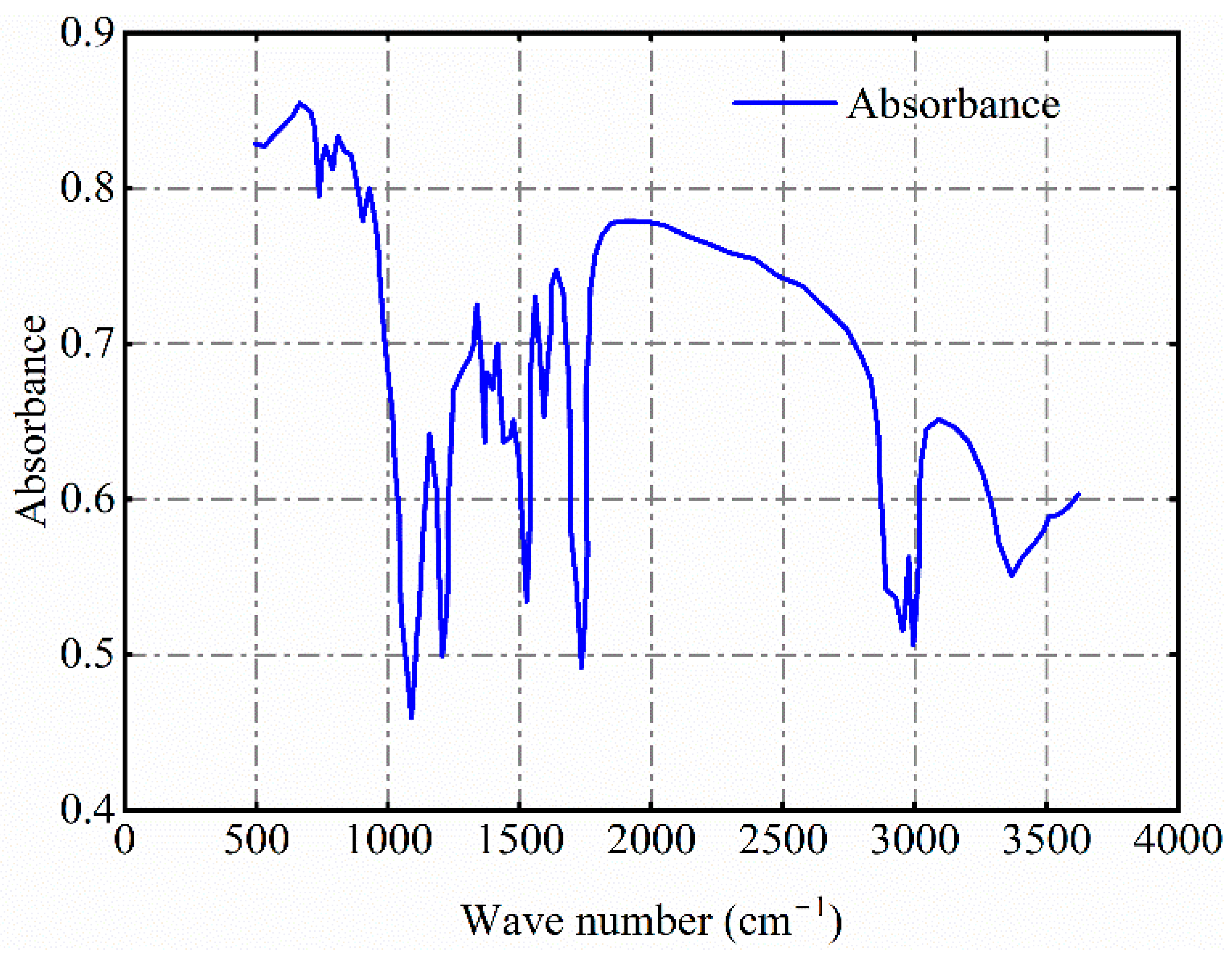
3.2. Data Source and Methodology

In the field of the electro-optical detection of objects in close proximity to space, target detection is often influenced by the atmosphere, primarily based on the following aspects.

(1) The radiative energy from both the target and background reaches the focal plane of the detector through the atmosphere, and the radiative signal undergoes atmospheric attenuation during the transmission.

(2) Bright sky background light constitutes the main background noise, diminishing the detection SNR and posing challenges for target detection. Hence, the analysis of the optical characteristics of the sky background is of significant importance.

The ERA5 reanalysis data and MODTRAN5 software were employed to simulate the atmospheric background transmittance and atmospheric background spectral radiance. In this study, the ERA5 data were used as input for the MODTRAN5 software to calculate the atmospheric background radiance.

The MODTRAN5 software serves as an atmospheric radiative transfer model with a medium spectral resolution. It inherits and improves the code of the LOWTRAN model, while incorporating an enhanced algorithm for multiple-scattering radiative transfer. Compared with LOWTRAN, it ensures the necessary precision and saves computational time compared with FASCODE. Therefore, using the radiative transfer calculation MODTRAN5 software allows the simulation and analysis of variations in sky radiance, thereby providing a basis for the theoretical analysis of optical detection systems for nearby spaces and low-speed targets. MODTRAN has established atmospheric models for various geographical locations, seasons, and climates. Its input interface is user-friendly, allowing custom inputs or the selection of weather condition modes suitable for various spectral ranges, such as ultraviolet, visible light, and infrared.

ERA5 was generated using the ECMWF Integrated Forecasting System (IFS) version CY41R2, utilizing 4D-Var data assimilation and model predictions. It consisted of 137 vertical hybrid σ/pressure (model) levels, with the top level positioned at 0.01 hPa. Specific information regarding the ERA5 data is presented in

Table 1. The specific information about the ERA5 data.

Horizontal Coverage	Horizontal Resolution	Vertical Resolution	Vertical Coverage	Temporal Coverage	Temporal Resolution
Global	0.25° × 0.25°	137 level	1000 hPa to 1 hPa	1959 to present	Hourly

. For detailed information, please refer to https://confluence.ecmwf.int/display/CKB/ERA5%3A+data+documentation (accessed on: 8 May 2024).

Figure 4 shows the simulated variations in temperature, relative humidity, and pressure with altitude in the South China Sea region during different seasons (DJF: December, January, February; MAM: March, April, May; JJA: June, July, August; and SON: September, October, November) in 2022.

According to Figure 4, in the South China Sea in 2022, the pressure change was not significant across the different seasons. The temperature exhibited considerable variation within the 1–5 km range, with a maximum of 5.2 K in DJF, 4.7 K in MAM, 5.36 K in JJA, and 1.98 K in SON. The relative humidity showed notable changes within the 20–40 km range, reaching a maximum of 9.3%, 11.84%, 8.1%, and 8% in DJF, MAM, JJA, and SON, respectively.

Taking DJF as an example, the relationship between the background radiance at an altitude of 20 km and atmospheric transmittance with respect to the wavelength variation is illustrated in Figure 5. It can be observed that within the 3–5 µm and 8–12 µm spectral bands, the background radiance is relatively low, while the atmospheric transmittance is high. Therefore, the detection of these two bands should be considered in future studies.

4. Result

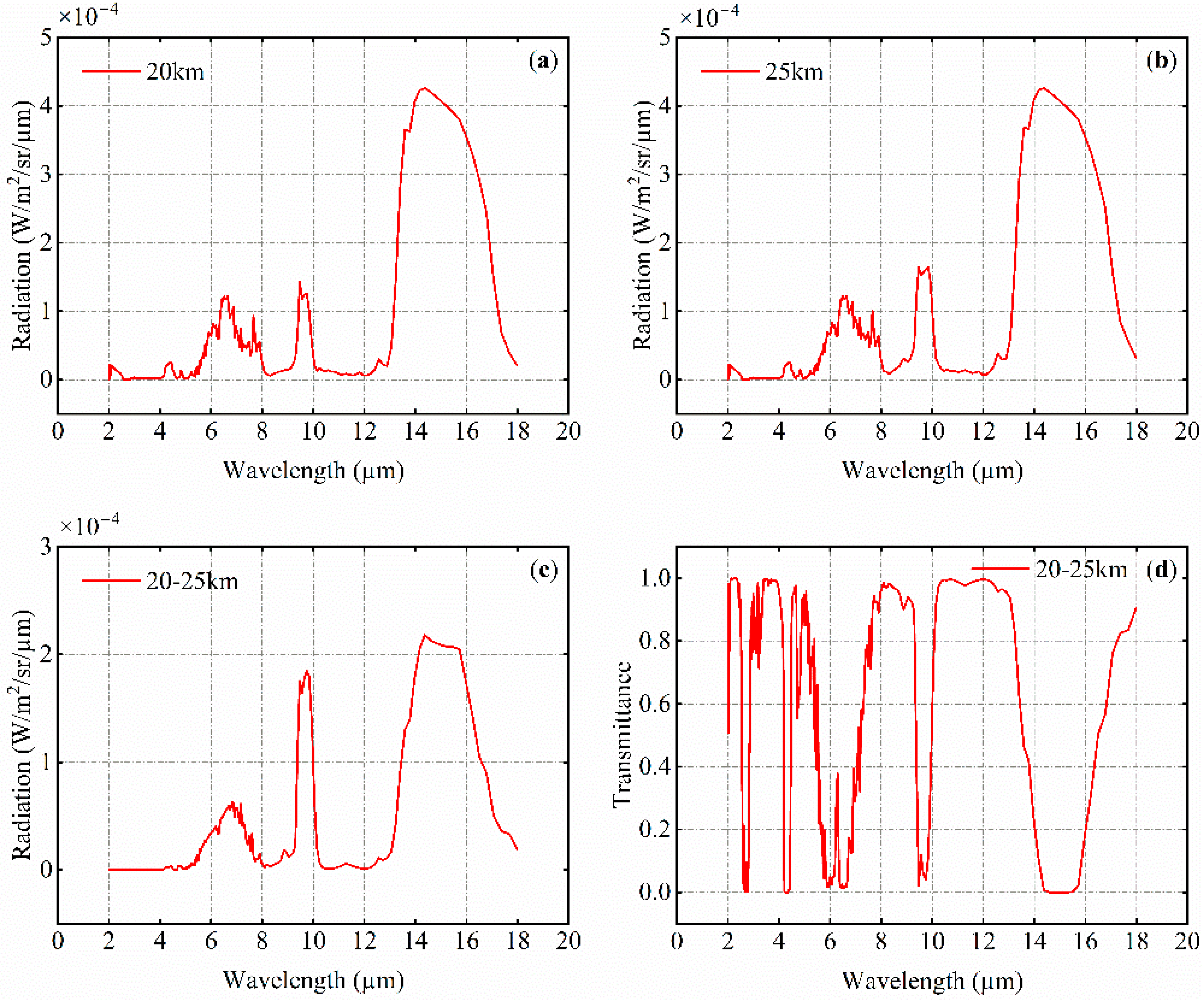
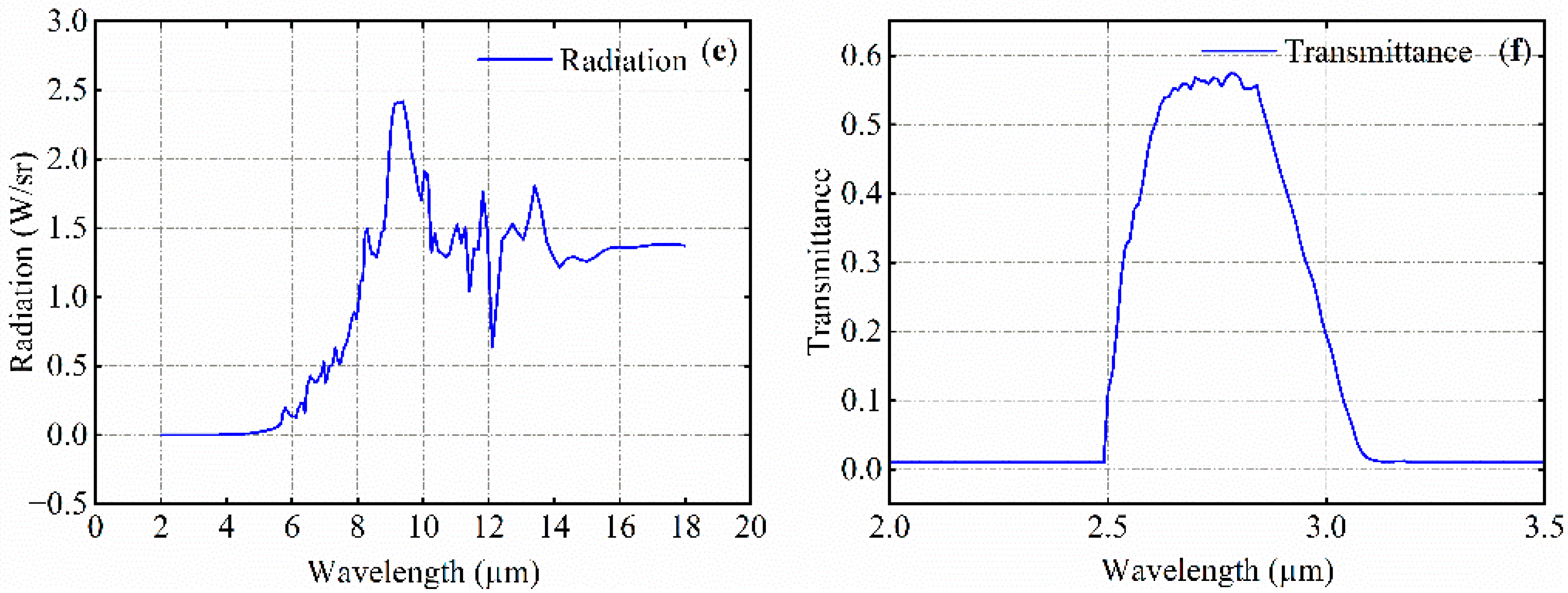
4.1. Verification of Thermal Characteristics of Stratospheric Airships

To validate the reliability of the thermal characteristic model for stratospheric airships, the computed results were compared to those reported by Kenya [32], as shown in Figure 6. For both the inner and outer surfaces, the skin material of the airship has solar absorptance of 0.33 and surface emissivity of 0.88. The experiments [32] were conducted in 2000 at a latitude of 36°N and ambient temperature of approximately 25.1 °C. The results indicated a consistent overall temperature trend, with a close agreement between the computed and experimental values at 10:00, 11:00, and 15:00.

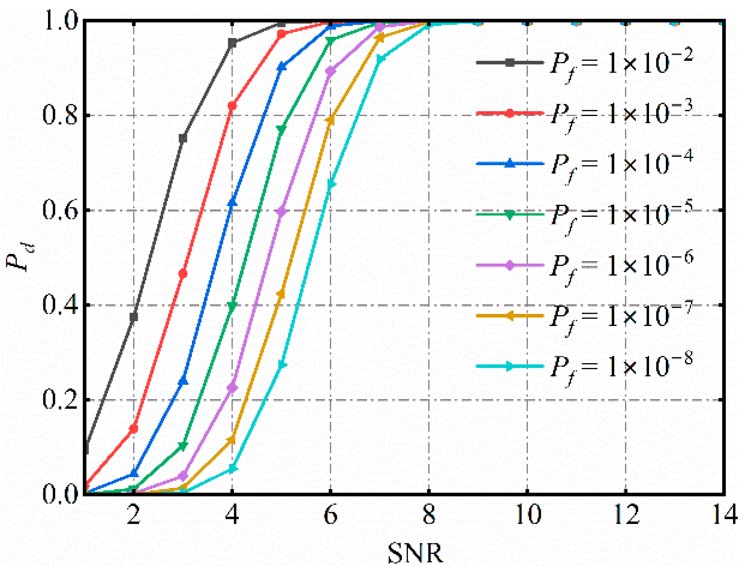
4.2. Optical Detection Conditions for Airships

Modern airships predominantly feature laminated composite materials on their surfaces [33]. The coating materials typically used for the outer surface are polyvinyl chloride (PVC), polytetrafluoroethylene (PTFE), and polyurethane coatings. Figure 7 shows the laboratory-measured IR spectrum of polyurethane polyester [34].

Selecting a particular airship target with a surface material consisting of a polyurethane coating, flying in the South China Sea region at an altitude of 20 km and observing at a height of 25 km, the system configuration parameters are as presented in the table below. The simulation begins at a wavelength (or central wavelength) precision of 1 nm, with corresponding band widths set at 0.01–0.3 µm for each starting wavelength (or central wavelength), with an interval of 0.01 µm for 30 bands. The system configuration parameters for the simulations are listed in

Table 2. System configuration parameters for simulations.

Parameters	Value
System optical aperture (mm)	360
System F-number	1.8
Focal length (mm)	650
Pixel pitch (µm)	25
Readout noise in electron counts	200
Fill factor	0.7
Quantum efficiency	0.6
Integration time (ms)	100 µs
Integration capacitor (pf)	0.2
Quantization bits	14
Full well capacity (e-)	3.5 × 106
Full well voltage (V)	2.8

. The SNR for the different seasons was calculated as in 2022.

Considering the example of DJF of 2022, Figure 8 illustrates the background radiance at a 20 km altitude, background radiance at a 25 km altitude, background radiance at a 20–25 km altitude, atmospheric transmittance at a 20–25 km altitude, target spectral radiance, and optical system transmittance.

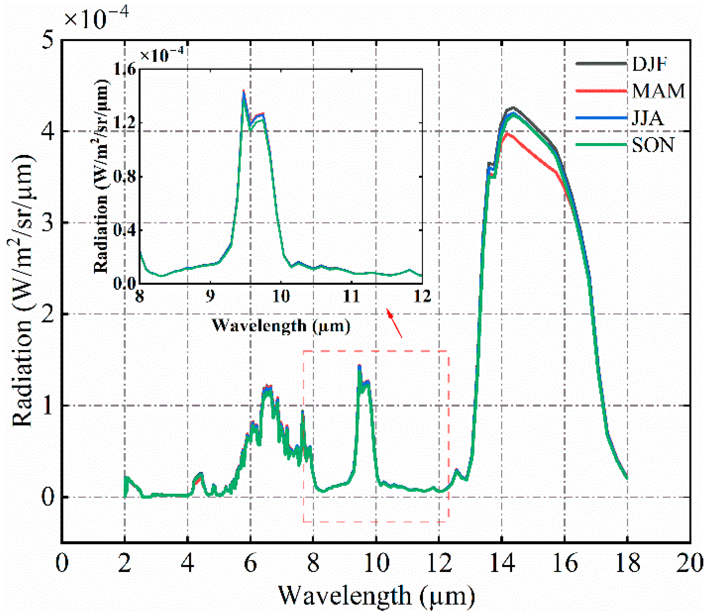
4.3. Simulation Results of Detection in Different Seasons

As an example of DJF of 2022, Figure 9, Figure 10, Figure 11 and Figure 12 present the relative relationship between the radiative flux on pixels, the signal electron counts on pixels in different spectral bands, the noise electron counts at different spectral bands, and the SNRs across various spectral bands.

The SNRs reach the maximum values at the central wavelengths of 8.83 µm, 10.83 µm, 11.51 µm, 12.39 µm, and 17.49 µm, as can be observed from Figure 12.

Table 3. SNRs for different detection bands.

Central Wavelength/µm	Starting Wavelength/µm	Ending Wavelength/µm	Bandwidth/µm	SNR
8.83	8.86	9.08	0.5	8.77
10.83	10.58	11.08	0.5	8.04
11.51	11.26	11.76	0.5	8.95
12.39	12.14	12.64	0.5	8.65
17.49	17.24	17.74	0.5	8.74

presents the SNRs at central wavelengths of 8.83 µm, 10.83 µm, 11.51 µm, 12.39 µm, and 17.49 µm with a bandwidth of 0.5 µm. It can be inferred that the SNR is the maximum at the central wavelength of 11.51 µm.

Figure 13 illustrates the spectral radiance of the airship in the South China Sea region during different seasons in 2022. As shown in Figure 13, the spectral radiance of the airship shows minimal variation across the four seasons in 2022 and the wavelengths corresponding to the peak values remain relatively constant.

Figure 14 displays the background radiance at an altitude of 20 km in the South China Sea region during different seasons in 2022.

In Figure 14, it can be observed that in the wavelength range of 6.55–7.37 µm, the background radiance is highest in MAM, lowest in DJF, and slightly higher in SON than in JJA. In the wavelength ranges of 2–6.54 µm and 9.94–18 µm, the background radiance is lowest in MAM, highest in DJF, and slightly higher in JJA than in SON. This is attributed to the altitude of 20 km, where higher temperatures in DJF and lower temperatures in MAM lead to corresponding variations in the background radiance.

Based on the simulation results for the DJF season (c.f. Table 3 and Figure 12), the SNR reaches its maximum at a center wavelength of 11.51 µm. As depicted by Figure 15, the SNRs for different seasons at a center wavelength of 11.51 µm are around a magnitude of 9.0.

One can seen that when the central wavelength is 11.51 µm, the SNR detected in MAM is maximized at 9.018, while the minimum SNR occurs in DJF at 8.955. The difference in the SNR between JJA and SON is not significant.

Considering a false alarm rate of 0.001%, simulations of the detection probability under different seasonal conditions were conducted, as illustrated in Figure 16.

As shown in Figure 16, the detection probability distributions are generally consistent across all four seasons. This uniformity arises from Figure 13 and Figure 14, in which the target spectral radiance and atmospheric background radiance exhibit consistent trends across the four seasons. These values differ only in magnitude within their respective wavelength bands. From Figure 16, it is evident that, under a false alarm rate of 0.001%, the detection probability first reaches 99% when the central wavelength is 8.83 µm with a bandwidth of 0.35 µm and when the central wavelength is 11.51 µm with a bandwidth of 0.34 µm.

5. Discussion

From the previous results and analysis in Section 4, it is found that the proposed model can effectively simulate the thermal characteristics of SA and obtain detection bands.

In reality, the thermal characteristic parameters of the skin material of SA may vary with temperature changes. Additionally, during actual experiments, the orientation of the airship and environmental parameters such as wind speed and direction may also change. These factors can all have an impact on the thermal characteristics of SA. As shown in Figure 6, there still exists a certain level of error between the calculation results and experimental results. With further research, we tend to explore a more accurate thermal characteristic model for SA in more complex thermodynamic environments.

In comparison to other detection models, we have employed a more systematic approach for selecting detection bands. This is explained by Figure 14, which indicates that, overall, the background radiance is lowest in MAM, highest in DJF, and slightly higher in SON than in JJA in the wavelength range of 0.2–18 µm. In addition, the signal radiance exhibits minimal variation. Therefore, the SNR is maximized in MAM. Based on the above analysis, the selection of a central wavelength of 8.83 µm with a bandwidth of 0.35 µm and a central wavelength of 11.51 µm with a bandwidth of 0.34 µm (i.e., 8.655–9.005 µm and 11.34–11.68 µm) is recommended. Additionally, based on the data provided, the detection of stratospheric airships is more feasible during MAM.

6. Conclusions

This study considers the thermal environment in which SA operate during flight. The exterior is affected by solar radiation, atmospheric infrared radiation, the Earth’s infrared radiation, and external convection, whereas the interior is affected by natural convection and infrared radiation between internal surfaces. A thermal characteristic calculation model for SA is established and simulations are conducted to emulate the thermal characteristics of SA in the South China Sea region. A detection system model for SA is established to identify the optimal detection bands for airship targets under specific backgrounds. This model includes the airship target signal, the atmospheric background signal, and mathematical models for the entire detection system. The false alarm rate and detection probability are used as evaluation indicators for the performance of the detection system. Simulations are conducted for SA in the South China Sea region under different seasonal conditions. The main conclusions are as follows.

(1) The skin temperature and radiation intensity of SA are primarily influenced by the solar radiation intensity, with lower values during the night and higher values during the day. Under floating conditions, both the skin temperature and radiation fields exhibit significant nonuniformity and considerable temporal variation.

(2) Under the condition of a 0.001% false alarm rate, the spectral bands of 8.655–9.005 µm and 11.34–11.68 µm are selected, making the optical detection of SA relatively more feasible.

(3) When the central wavelengths are 8.83 µm and 11.51 µm, the SNR is maximized in MAM and minimized in DJF, and the SNR difference between JJA and SON is not significant. The optical detection of SA is more feasible in MAM because of the higher SNR during this season.

References

1. Dolce, J.L.; Collozza, A. High-Altitude, Long-Endurance Airships for Coastal Surveillance. 2005. Available online: https://ntrs.nasa.gov/citations/20050080709 (accessed on 20 May 2024).
2. Jamison, L.; Sommer, G.; Porche, I. High-Altitude Airships for the Future Force Army; Rand: Santa Monica, CA, USA, 2005. [Google Scholar]
3. SantaPietro, J.J. Persistent Wide Area Surveillance from an Airship. IEEE Aerosp. Electron. Syst. Mag. 2012, 27, 11–16. [Google Scholar] [CrossRef]
4. Ilieva, G.; Páscoa, J.; Dumas, A.; Trancossi, M. MAAT—Promising innovative design and green propulsive concept for future airship’s transport. Aerosp. Sci. Technol. 2014, 35, 1–14. [Google Scholar] [CrossRef]
5. Smith, I.; Lee, M.; Fortneberry, M.; Judy, R. HiSentinel80: Flight of a high altitude airship. In Proceedings of the 11th AIAA Aviation Technology, Integration, and Operations (ATIO) Conference, Including the AIAA Balloon Systems Conference and 19th AIAA Lighter-Than, Virginia Beach, VA, USA, 20–22 September 2011; p. 6973. [Google Scholar]
6. Androulakakis, S.P.; Judy, R. Status and plans of high altitude airship (HAATM) program. In Proceedings of the AIAA Lighter-Than-Air Systems Technology (LTA) Conference, Daytona Beach, FL, USA, 25–28 March 2013; p. 1362. [Google Scholar]
7. Bonnici, M.; Tacchini, A.; Vucinic, D. Long permanence high altitude airships: The opportunity of hydrogen. Eur. Transp. Res. Rev. 2014, 6, 253–266. [Google Scholar] [CrossRef]
8. Hygounenc, E.; Jung, I.K.; Souères, P.; Lacroix, S. The autonomous blimp project of LAAS-CNRS: Achievements in flight control and terrain mapping. Int. J. Robot. Res. 2004, 23, 473–511. [Google Scholar] [CrossRef]
9. Kusagaya, T.; Kojima, H.; Fujii, H.A. Estimation of flyable regions for planetary airships. J. Aircr. 2006, 43, 1177–1181. [Google Scholar] [CrossRef]
10. Schmidt, D.K.; Stevens, J.; Roney, J. Near-space station-keeping performance of a large high-altitude notional airship. J. Aircr. 2007, 44, 611–615. [Google Scholar] [CrossRef]
11. Lei, C.; Cheng, L.; Kavanagh, K. Spanwise length effects on three-dimensional modelling of flow over a circular cylinder. Comput. Meth. Appl. Mech. Eng. 2001, 190, 2909–2923. [Google Scholar] [CrossRef]
12. Kreith, F.; Kreider, J.F. Numerical Prediction of the Performance of High Altitude Balloons; NCAR Technical Note NCAR-TN/STR-65; National Center for Atmospheric Research: Boulder, CO, USA, 1974. [Google Scholar]
13. Khoury, G.A. Airship Technology; Cambridge University Press: Cambridge, UK, 2012; Volume 10. [Google Scholar]
14. Carlson, L.A.; Horn, W.J. New Thermal and Trajectory Model for High-Altitude Balloons. J. Aircr. 1983, 20, 500–507. [Google Scholar] [CrossRef]
15. Louchev, O.A. Steady-State Model for the Thermal Regimes of Shells of Airships and Hot Air Balloons. Int. J. Heat Mass Transf. 1992, 35, 2683–2693. [Google Scholar] [CrossRef]
16. Farley, R. BalloonAscent: 3-D simulation tool for the ascent and float of high-altitude balloons. In Proceedings of the AIAA 5th ATIO and16th Lighter-Than-Air Sys Tech. and Balloon Systems Conferences, Arlington, VA, USA, 26–28 September 2005; p. 7412. [Google Scholar]
17. Xia, X.L.; Li, D.F.; Sun, C.A.; Ruan, L.M. Transient thermal behavior of stratospheric balloons at float conditions. Adv. Space Res. 2010, 46, 1184–1190. [Google Scholar] [CrossRef]
18. Liu, Q.; Wu, Z.; Zhu, M.; Xu, W.Q. A comprehensive numerical model investigating the thermal-dynamic performance of scientific balloon. Adv. Space Res. 2014, 53, 325–338. [Google Scholar] [CrossRef]
19. Shi, H.; Song, B.Y.; Yao, Q.P.; Cao, X. Thermal Performance of Stratospheric Air-ships During Ascent and Descent. J. Thermophys. Heat Transf. 2009, 23, 816–821. [Google Scholar] [CrossRef]
20. Stefan, K. Thermal effects on a high altitude airship. In Proceedings of the 5th Lighter-Than Air Conference, Anaheim, CA, USA, 25–27 July 1983; p. 1984. [Google Scholar]
21. Franco, H.; Cathey, H.M. Thermal performance modeling of NASA’s scientific balloons. In Next Generation in Scientific Ballooning; Jones, W.V., Ed.; Advances in Space Research; Pergamon-Elsevier Science Ltd.: Kidlington, UK, 2004; Volume 33, pp. 1717–1721. [Google Scholar]
22. Dong, Y.C.; Chen, F.S.; Wang, Y.; Su, X.F.; Wang, W. A Limb Atmospheric Radiance Inversion Method based on a Sun-synchronous Orbit Satellite. In Proceedings of the 2nd International Seminar on High-Power Laser Interaction with Matter and Application/International Seminar on Space Surveillance Technology/2nd Symposium on Combustion Diagnostics, Suzhou, China, 19–24 October 2014. [Google Scholar]
23. Han, Y.; Xuan, Y. The Study and Application of the IR Feature of Target and Background. Infrared Technol. 2002, 24, 16–19. [Google Scholar]
24. Han, Y.; Xuan, Y. Effect of atmospheric transmission on irradiation feature of target and background. J. Appl. Opt. 2002, 4, 8–11. [Google Scholar]
25. Zong, J.; Zhang, J.; Liu, D. Infrared Radiation Characteristics of the Stealth Aircraft. Acta Photonica Sin. 2011, 40, 289–294. [Google Scholar] [CrossRef]
26. Si-Li, G.; Xin-Yi, T. Building model of the plume released from the flying machine and simulation. Opto-Electron. Eng. 2007, 34, 25–27. [Google Scholar]
27. Karlholm, J.; Renhorn, I. Wavelength band selection method for multispectral target detection. Appl. Opt. 2002, 41, 6786–6795. [Google Scholar] [CrossRef] [PubMed]
28. Ni, X.; Yu, S.; Su, X.; Chen, F. Detection spectrum optimization of stealth aircraft targets from a space-based infrared platform. Opt. Quantum Electron. 2022, 54, 151. [Google Scholar] [CrossRef]
29. Liu, F.; Shao, X.P.; Han, P.L.; Bin, X.; Yang, C. Detection of infrared stealth aircraft through their multispectral signatures. Opt. Eng. 2014, 53, 10. [Google Scholar] [CrossRef]
30. Wang, Y.; Huang, S.; Liu, D.; Wang, B. Novel band selection method based on target detection. Infrared Laser Eng. 2013, 42, 2294–2298. [Google Scholar]
31. Lin, T.; Liu, F.; Wang, Y.; Zhang, J. Band performance analysis method of spectrum detection about infrared stealth aircraft. J. Xidian Univ. 2016, 43, 54–59+81. [Google Scholar] [CrossRef]
32. Harada, K.; Eguchi, K.; Sano, M.; Sasa, S. Experimental study of thermal modeling for stratospheric platform airship. In Proceedings of the AIAA’s 3rd Annual Aviation Technology, Integration, and Operations (ATIO) Forum, Denver, CO, USA, 17–19 November 2003; p. 6833. [Google Scholar]
33. Li, H.; He, J.-Y.; Na, S. Research on Thermal Performance of a Stratospheric Airship at High-Altitude Station-Keeping Conditions. J. Xi’an Aeronaut. Univ. 2016, 34, 7–12+43. [Google Scholar]
34. Zhi, J.; Yuan, K.J.; Li, S.F.; Chow, W.K. Study of FTIR spectra and thermal analysis of polyurethane. Spectrosc. Spectr. Anal. 2006, 26, 624–628. [Google Scholar]
Figure 1. Thermodynamic environment of stratospheric airships.
Remotesensing 16 01884 g001
Figure 2. Instantaneous field of view imaging schematic when the target forms an image as a single pixel.
Remotesensing 16 01884 g002
Figure 3. The relationship between the SNR and the detection probability and false alarm rate.
Remotesensing 16 01884 g003
Figure 4. The variations in the temperature, relative humidity, and pressure with the altitude. (a1) The temperature of DJF; (a2) The relative humidity of DJF; (a3) The pressure of DJF; (b1) The temperature of MAM; (b2) The relative humidity of MAM; (b3) The pressure of MAM; (c1) The temperature of JJA; (c2) The relative humidity of JJA; (c3) The pressure of JJA; (d1) The temperature of SON; (d2) The relative humidity of SON; (d3) The pressure of SON.
Remotesensing 16 01884 g004aRemotesensing 16 01884 g004b
Figure 5. The variation in background radiance and atmospheric transmittance with the wavelength at an altitude of 20 km.
Remotesensing 16 01884 g005
Figure 6. Model validation. (a) Comparison between the calculation results and experimental results [32]; (b) error bar graph of the calculation results.
Remotesensing 16 01884 g006
Figure 7. Laboratory-measured IR spectrum of polyurethane polyester [34].
Remotesensing 16 01884 g007
Figure 8. (a) Background radiance at 20 km altitude; (b) background radiance at 25 km altitude; (c) background radiance from 20 to 25 km altitude; (d) atmospheric transmittance from 20 to 25 km altitude; (e) spectral radiance of target; (f) optical transmittance.
Remotesensing 16 01884 g008aRemotesensing 16 01884 g008b
Figure 9. The relative relationship of the radiative flux on the pixel.
Remotesensing 16 01884 g009
Figure 10. The signal electron counts on the pixel in different spectral bands.
Remotesensing 16 01884 g010
Figure 11. The temporal noise electron counts on the pixel in different spectral bands.
Remotesensing 16 01884 g011
Figure 12. The SNRs in different spectral bands.
Remotesensing 16 01884 g012
Figure 13. The spectral radiance of the airship during different seasons.
Remotesensing 16 01884 g013
Figure 14. The seasonal variation in the background radiance at a 20 km altitude.
Remotesensing 16 01884 g014
Figure 15. SNRs for different seasons at detection band with central wavelength of 11.51 µm.
Remotesensing 16 01884 g015
Figure 16. Detection probability under different seasonal conditions. (a) DJF; (b) MAM; (c) JJA; (d) SON.
Remotesensing 16 01884 g016