Unveiling Glacier Mass Balance: Albedo Aggregation Insights for Austrian and Norwegian Glaciers

Abstract

Assessing the regional mass balance of European glaciers presents significant challenges due to limited measurements. While various albedo methods have been explored for individual glaciers, a comprehensive analysis of aggregated albedo methods is lacking. Addressing this gap, in our study, we examined five MODIS aggregated albedos (raw average, minimum average, average minimum, interpolated average, and cumulative) versus the annual mass balance for 12 Austrian and Norwegian glaciers from 2001 to 2020 to establish connections between them. We find that the raw average albedo is strongly correlated with the annual mass balance of Austrian glaciers (r = 0.91), while the interpolated average albedo is significantly correlated with the annual mass balance of Norwegian glaciers (r = 0.90). Moreover, we observe that high-elevation glaciers experience fewer cloud cover days, allowing the raw average albedo to reliably estimate the annual mass balance, whereas low-elevation glaciers are often obscured by clouds, potentially masking the true minimum albedo. Additionally, traditional indicators, such as the equilibrium-line altitude and accumulation area ratio, exhibit significant correlations with the annual mass balance of Norwegian and Austrian glaciers (r = 0.90 and 0.87, respectively), yet albedo demonstrates higher robustness. These findings provide a reference for selecting appropriate aggregation methods to reconstruct glacier mass balance from albedo observations.

1. Introduction

Glaciers are of paramount importance in the Earth’s climate system, acting as vital reservoirs of freshwater and significantly influencing regional hydrology patterns [1]. The concept of glacier mass balance, representing the net gain or loss of ice over a specific time frame, stands as a key metric for gauging glacier response to climatic shifts. Observing long-term changes in glacier mass balance is critical for predicting future changes and assessing their impact on water resources and sea levels [2].

Numerous techniques have been employed to quantify glacier mass balance, encompassing field measurements, mass balance models, geodetic surveys, and glacier surface characteristic approaches [3]. Some scholars have calibrated mass balance models using field-based mass balance measurements [4,5] to decipher long-term mass balance trends [6]. However, field measurements are less applicable in harsh and inaccessible terrains. In recent years, geodetic techniques based on remote sensing data have facilitated the computation of glacier surface elevation alterations and corresponding mass balance shifts [7,8]. These approaches offer the possibility of estimating annual or seasonal mass balance dynamics [9,10]. Glacier surface characteristic approaches, such as the accumulation area ratio (AAR) [11,12,13], equilibrium-line altitude (ELA) [14,15], albedo [16,17,18,19], and thickness change [20], have also been harnessed for mass balance assessments due to their computability from multisource remote sensing data with a heightened temporal resolution, for example, Landsat, Moderate Resolution Imaging Spectroradiometer (MODIS) and Advanced Very High-Resolution Radiometer (AVHRR) data. Consequently, these methodologies have been applied to estimate annual or seasonal mass balance changes in glaciated areas [21].

Surface albedo is a key determinant of the energy balance and directly affects glacier mass balance [22,23,24,25]. The intricate relationship between glacier albedo and mass balance has attracted increased attention in recent years, prompting studies of various approaches to understand this connection. For instance, Greuell et al. [26] proposed a method for the Svalbard archipelago, estimating absorbed radiation levels based on measured albedo data and meteorological observations. Subsequently, the use of this method led to the establishment of a correlation between absorbed radiation and glacier mass balance. However, its reliance on on-site radiation measurements limits its applicability in broader-scale investigations.

An alternative approach involves satellite-based measurements of a glacier’s albedo, which are then merged into a single value for the whole glacier using an albedo aggregation technique. This approach aims to examine the association between the annual mass balance and glacier albedo averages during the melt season (June, July, August). These aggregation methods encompass the raw average albedo [27], minimum average albedo [28], average minimum albedo [18], interpolated average albedo [27], and cumulative albedo [29]. For instance, the minimum average albedo of the Brewster Glacier in New Zealand [30], the average minimum albedo of the Muz Taw Glacier in the Altai Mountains [31], and the interpolated average albedo of glaciers in the Canadian Arctic [27] all demonstrate statistically significant correlations with glacier mass balance.

Previous research has highlighted a strong correlation between albedo and glacier mass balance, suggesting the potential for reconstructing glacier mass balance using albedo data. However, different albedo aggregation methods exhibit varying performances. The use of daily MODIS albedo data by Sirguey et al. [29] showed variability in the correlation between average minimum albedo and mass balance. Their findings indicate that the raw average albedo during the melt season exhibits a stronger correlation with summer mass balance compared to the minimum average albedo. This suggests that the glacier-wide minimum albedo may not be the best aggregation method for glacier mass balance estimates, as clouds may obscure the true minimum albedo value. Greuell and Oerlemans [32] pointed out that the minimum albedo method is well-suited for glaciers with small accumulation rates. For larger glaciers, the interpolated average albedo method has better applicability than the raw or minimum average albedo method [27]. Furthermore, different types of glaciers exhibit different correlations between albedo and mass balance. For instance, Dumont et al. [18] found a strong linear correlation between the minimum average albedo value and the mass balance of temperate glaciers. Sirguey et al. [29] confirmed that average minimum albedo is a reliable predictor of annual mass changes in maritime glaciers. Zhang et al. [33] evaluated the applicability of the albedo-based method to continental glaciers on the Tibetan Plateau and found a significant linear correlation between the annual average minimum albedo and mass balance. However, most current studies focus on analyzing glaciers within specific regions or countries, overlooking the potential differences in mass balance and albedo response among glaciers in different climates. Therefore, there is a need to comprehensively analyze both continental and maritime glaciers and systematically assess the suitability of various aggregated albedo methods for estimating glacier mass balance. In this study, we chose to study Austria and Norway, two representative regions in glacier research, to analyze the time series characteristics of glacier albedo and mass balance. Our aim is to explore the applicability of different albedo aggregation methods to measure changes in glacier mass balance within these regions.

To explore the correlation between aggregated albedo and the annual mass balance, the objectives of this study are as follows: (1) to analyze time-series variations in mass balance and albedo over nearly two decades in the studied glaciers, (2) to evaluate the ability of different albedo aggregation methods for estimating changes in glacier mass balance, and (3) to explore the potential reasons for differences in the performance of aggregation methods. In this study, we aim to deepen the understanding of the interaction between albedo and glacier mass balance and improve the ability to assess the response of small- and medium-sized glaciers to mass balance changes.

2. Study Area and Data

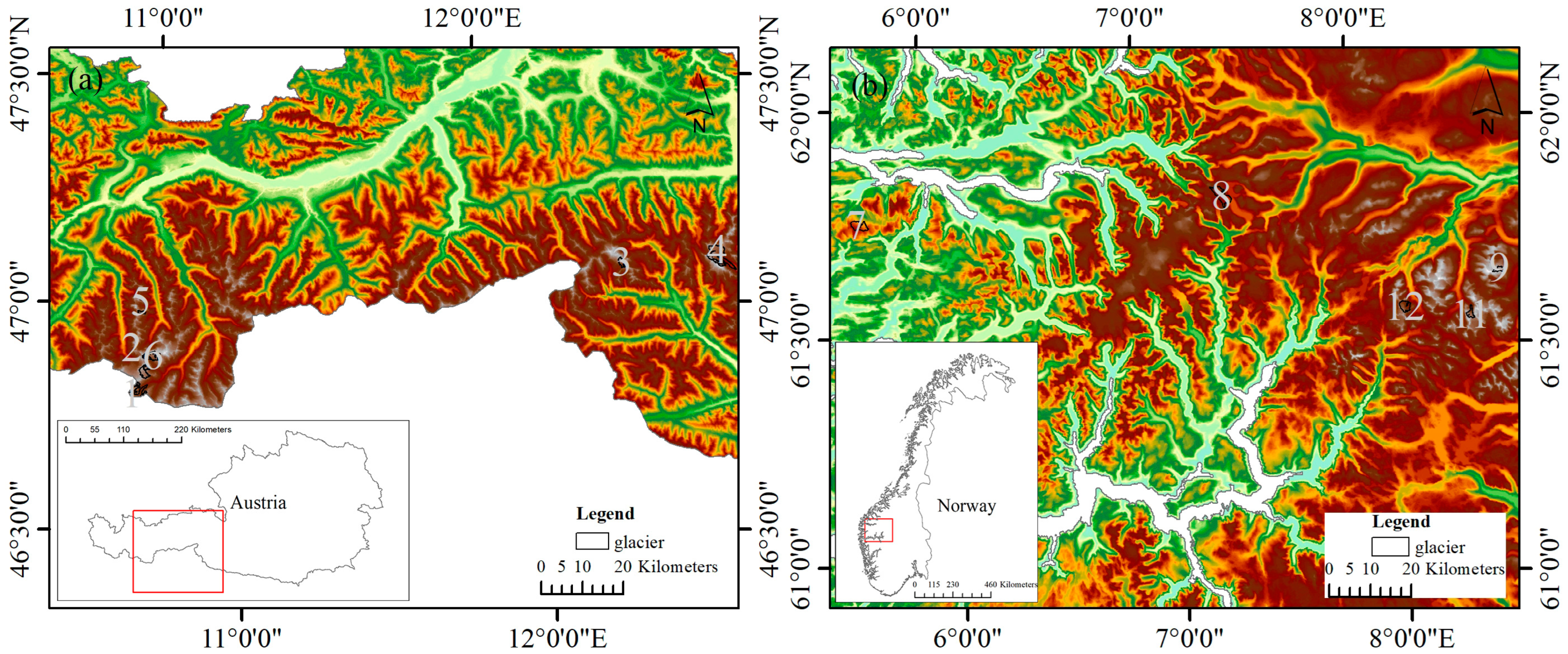
2.1. Study Area

Glaciers in continental Europe cover an area of approximately 5000 square kilometers, with a total ice volume of around 400 cubic kilometers. They are predominantly found in high-altitude regions such as the Alps, the Greater Caucasus Mountains, the Pyrenees, and high-latitude areas of the Scandinavian Peninsula in Norway and Sweden [34,35]. Since the 19th century, although some glaciers have occasionally exhibited a positive short-term mass balance, the overall trend across continental Europe has been a continuous retreat, with an increasing rate of recession [36]. Previous studies have predicted a significant glacier melting in the Alps by the end of this century, with a substantial loss of small glaciers and at least 80–90% mass loss in some larger glaciers [37].

This negative trend in the annual mass balance observed in the European Alps over the last three decades is largely attributed to increased summer melting, driven by heightened surface energy fluxes [38] and an extended ablation season [39]. Year-to-year variations are influenced by albedo feedback effects, which are, in turn, influenced by regional meteorological conditions and winter snow cover differences [40]. Surface albedo plays a significant role in modulating snow and ice ablation, with small differences in accumulation rates leading to pronounced variations in ablation. The distribution of winter precipitation across the Austrian glacier zone varies, with higher precipitation in the easternmost and westernmost regions compared to the central area. Drier climates result in earlier exposure of bare ice and prolonged ablation periods. Consequently, glaciers in drier climates are expected to lose more mass than those in wetter climates under similar warming conditions [41]. Norwegian glaciers, situated in a maritime climate, are highly sensitive to climate fluctuations, with the mass balance heavily influenced by large-scale atmospheric circulation patterns [42]. The relatively high winter precipitation and the smaller difference between average winter and summer temperatures in Norway make it an ideal location to study glacier responses to climate change [43].

In this study, we selected 12 glaciers in Austria and Norway (Figure 1,

Table 1. Information on glaciers in Norway and Austria in this study.

ID	Name	Country	Lon	Lat	Elevation Range (m)	Area (km2)	Available Time	Glacier Type
1	Hintereis F	Austria	10.77	46.8	2547, 3714	6.14	1953–2020	continental
2	Kesselwand F	Austria	10.79	46.84	2890, 3497	3.55	1953–2020	continental
3	Mullwitz K	Austria	12.38	47.08	2450, 3470	2.56	2007–2020	continental
4	Pasterze	Austria	12.7	47.1	2000, 3600	15.34	1980–2020	continental
5	Seekarles F	Austria	10.82	46.98	2740, 3255	1.04	2014–2020	continental
6	Vernagt F	Austria	10.82	46.88	2872, 3585	6.89	1965–2020	continental
7	Aalfotbreen	Norway	5.65	61.75	890, 1368	3.48	1963–2020	maritime
8	Austdalsbreen	Norway	7.35	61.82	1200, 1740	10.62	1988–2020	maritime-continental
9	Graasubreen	Norway	8.6	66.66	1850, 2277	8.05	1962–2020	continental
10	Hansebreen	Norway	5.68	61.75	927, 1310	2.48	1986–2020	maritime
11	Hellstugubreen	Norway	8.44	61.56	1487, 2213	2.66	1962–2020	continental
12	Storbreen	Norway	8.13	61.57	1420, 2091	4.88	1949–2020	maritime-continental

). These glaciers have a diverse range of surface areas, ranging from approximately 1 to 16 square kilometers, thus providing an ideal spatial scale for unraveling the intricate relationship between surface albedo and mass balance. A key consideration in the glacier selection was the availability of long-term data and adequate spatial coverage, ensuring the reliability of the analytical outcomes. This deliberate diversity enables us to effectively capture the nuanced responses of albedo and mass balance to regional environmental factors.

2.2. Study Data

2.2.1. Terra/Aqua MODIS Albedo

The albedo data utilized in this study are derived from the MOD10A1 product with a temporal resolution of 1 day and a spatial resolution of 500 m. The normalized difference snow index (NDSI) was initially calculated to distinguish snow/ice from land areas. Subsequently, the MODIS cloud mask was applied to identify cloudy cells, followed by a series of tests to screen grid cells with uncertain factors such as a low NDSI or a high solar zenith angle. For grid cells clearly identified as snow/ice, the albedo was then calculated using the best daily swath observations and applying an anisotropy correction factor [44].

Numerous previous studies have demonstrated the reliability of MODIS albedo data in glacial regions by showing good consistency with in situ measurements [45,46]. Therefore, in this study, we rely on MOD10A1 albedo data to investigate the relationship between summer albedo and the annual mass balance of small and medium-sized glaciers.

2.2.2. Glacier Mass Balance

The World Glacier Monitoring Service (WGMS) is a globally recognized institution committed to the comprehensive compilation of glacier-related data on a global scale. It systematically collects extensive and precise glacier monitoring data, including complex records of mass balance, glacier area, and ELA data. For more detailed information, interested parties can refer to the official WGMS website: https://wgms.ch/ (accessed on 3 April 2024).

Within the MODIS observation period spanning from 2001 to 2020, our analysis focuses on 12 glaciers selected based on the WGMS database. The primary emphasis lies in extracting annual mass balance values exclusively within well-defined glacier boundaries. Figure 2 shows the cumulative annual mass balance changes of the studied glaciers, revealing a consistent pattern of mass balance reduction across all considered glaciers. Notably, the glacier mass balance demonstrates a significant and faster decline in the Austrian region compared to the Norwegian region. This phenomenon has persisted since the beginning of the 21st century.

3. Methods

In this study, the glaciated areas are predominantly mountainous, and shaded regions were excluded to avoid incorporating unrealistically low albedo values [47,48,49]. Values below 0.05 were deemed as influenced by shadows and were consequently excluded from the analysis. Additionally, a challenge arises in distinguishing between bright, dry snow and clouds, which may exhibit similar albedos in satellite reflectance [50]. To mitigate the potential misclassification of snow, we filtered the MOD10A1 daily albedo product using the expected range of glacial snow and ice albedo [51]. Values exceeding 0.99, considered physically impractical for snow or glaciers [27], were excluded.

Based on these filtered MOD10A1 daily snow albedo data, we employed five aggregation methods to determine a single average albedo value for each glacier during summer:

A.

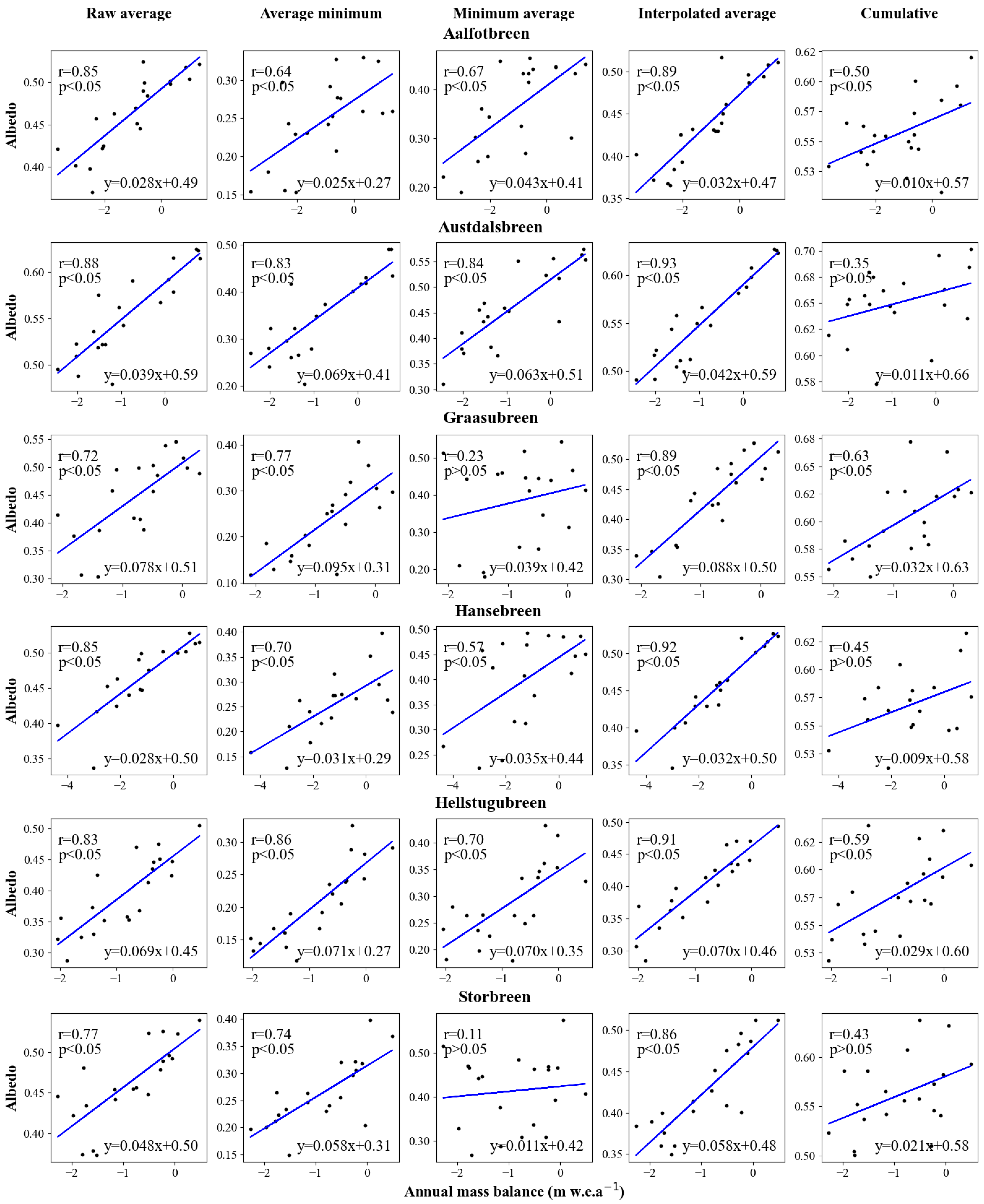
The raw average method: The calculation of the average albedo for the months of June, July, and August involves aggregating all accessible albedo values for each grid cell within the glacier profile, excluding cells with cloud cover. Subsequently, an equally weighted average is calculated to combine these values into a single albedo representation for each glacier in each year. The specific calculation formula is as follows:

$${\overline{\alpha }}_i=({\sum }_{\mathrm{doy}=152}^{\mathrm{doy}=243}{\alpha }_i\left(\mathrm{d}\mathrm{o}\mathrm{y}\right))/m$$

(1)

$${\alpha }_{raw\_average}=({\sum }_{i=1}^{i=n}{\overline{\alpha }}_i)/n$$

(2)

where ${\alpha }_i\left(\mathrm{d}\mathrm{o}\mathrm{y}\right)$ represents the albedo of the $i$-th pixel on a certain day, m represents the effective albedo number of the $i$-th pixel, and n represents the total number of pixels of the glacier. ${\overline{\alpha }}_i$ represents the average albedo of the $i$-th pixel, and ${\alpha }_{raw\_average}$ represents the raw average albedo.

B.

The minimum average method: For each glacier, we computed the average albedo value and cloud cover for each day within a specific time period. From the sequence of average albedo values, we selected the minimum value that meets the cloud cover threshold. In this study, the cloud cover threshold was set at 20% after considering the cloud cover conditions in the study area [29]. The specific calculation formula is as follows:

$$\overline{\alpha }\left(\mathrm{d}\mathrm{o}\mathrm{y}\right)=({\sum }_{i=1}^{i=n}{\alpha }_i\left(\mathrm{d}\mathrm{o}\mathrm{y}\right))/n$$

(3)

$${\alpha }_{minimum\_average}=\min \{\overline{\alpha }\left(\mathrm{d}\mathrm{o}\mathrm{y}\right),152\le \mathrm{d}\mathrm{o}\mathrm{y}\le 243\}$$

(4)

where $\overline{\alpha }\left(\mathrm{d}\mathrm{o}\mathrm{y}\right)$ represents the average albedo on a certain day, and ${\alpha }_{minimum\_average}$ represents the minimum average albedo.

C.

The average minimum method: Within the glacier’s outline, the minimum albedo value for each pixel was determined, producing a map of the minimum albedo for each glacier. We then obtained the aggregated value by calculating the average of all pixel minimum albedo values using an equal-weight averaging method. The specific calculation formula is as follows:

$${\alpha }_i^{min}=\min \left\{{\alpha }_i\left(\mathrm{d}\mathrm{o}\mathrm{y}\right),152\le \mathrm{d}\mathrm{o}\mathrm{y}\le 243\right\}$$

(5)

$${\alpha }_{average\_minimum}=({\sum }_{i=1}^{i=n}{\alpha }_i^{min})/n$$

(6)

where ${\alpha }_i^{min}$ represents the minimum albedo value of the $i$-th pixel, and ${\alpha }_{average\_minimum}$ represents the average minimum albedo.

D.

The interpolated average method: To address missing (cloudy) pixels within the glacier, linear interpolation was employed to fill the albedo time series for each pixel. Similar to the raw average method, an equal-weighted averaging approach is then utilized to compute an interpolated average albedo for each pixel, which is subsequently weighted to obtain an aggregated albedo for each glacier, and calculated as follows:

$${\alpha }_{interpolated\_average}=({\sum }_{i=1}^{i=n}{\overline{\alpha }}_i^{interpolation})/n$$

(7)

where ${\overline{\alpha }}_i^{interpolation}$ represents the average albedo of the $i$-th pixel after linear interpolation, and ${\alpha }_{interpolated\_average}$ represents the interpolated average albedo.

E.

The cumulative method: Similar to the interpolated average method, the albedo time series data were interpolated to fill cloud pixels. Subsequently, the average albedo data for all pixels were computed using the equal-weighted averaging method. However, instead of deriving an equal-weighted average of the aggregated values, the accumulation method uses integration to obtain the aggregated albedo for each glacier, which is calculated as follows:

$${\alpha }_{cumulative}=({\int }_{\mathrm{doy}=152}^{\mathrm{doy}=243}{\overline{\alpha }}^{interpolation}(\mathrm{doy}))/92$$

(8)

where ${\overline{\alpha }}^{interpolation}(\mathrm{doy})$ represents the average albedo value after linear interpolation on a certain day, and ${\alpha }_{cumulative}$ represents the cumulative albedo. The number 92 represents the total days in summer, encompassing June, July, and August.

The raw average method offers a straightforward portrayal of the average albedo during the summer months, while the minimum average method helps identify periods of minimum albedo values, which are correlated with increased ablation rates. The average minimum method highlights the spatial distribution of minimum albedo values within a glacier area, and the interpolated average method addresses data gaps caused by cloud cover, ensuring a more comprehensive representation of albedo variations. Lastly, the cumulative method integrates albedo data over time, providing insights into the cumulative energy absorption by the glacier. By employing these methods, we aim to thoroughly evaluate the impact of albedo on glacier mass balance.

Next, standard least squares linear regression was performed on the annual aggregated albedo values obtained using the five methods and the corresponding mass balance data. This analysis aims to clarify the correlation between summer albedo and mass balance, providing insights into the performance of these aggregation methods in scaling the mass balance of European maritime and continental glaciers.

4. Results

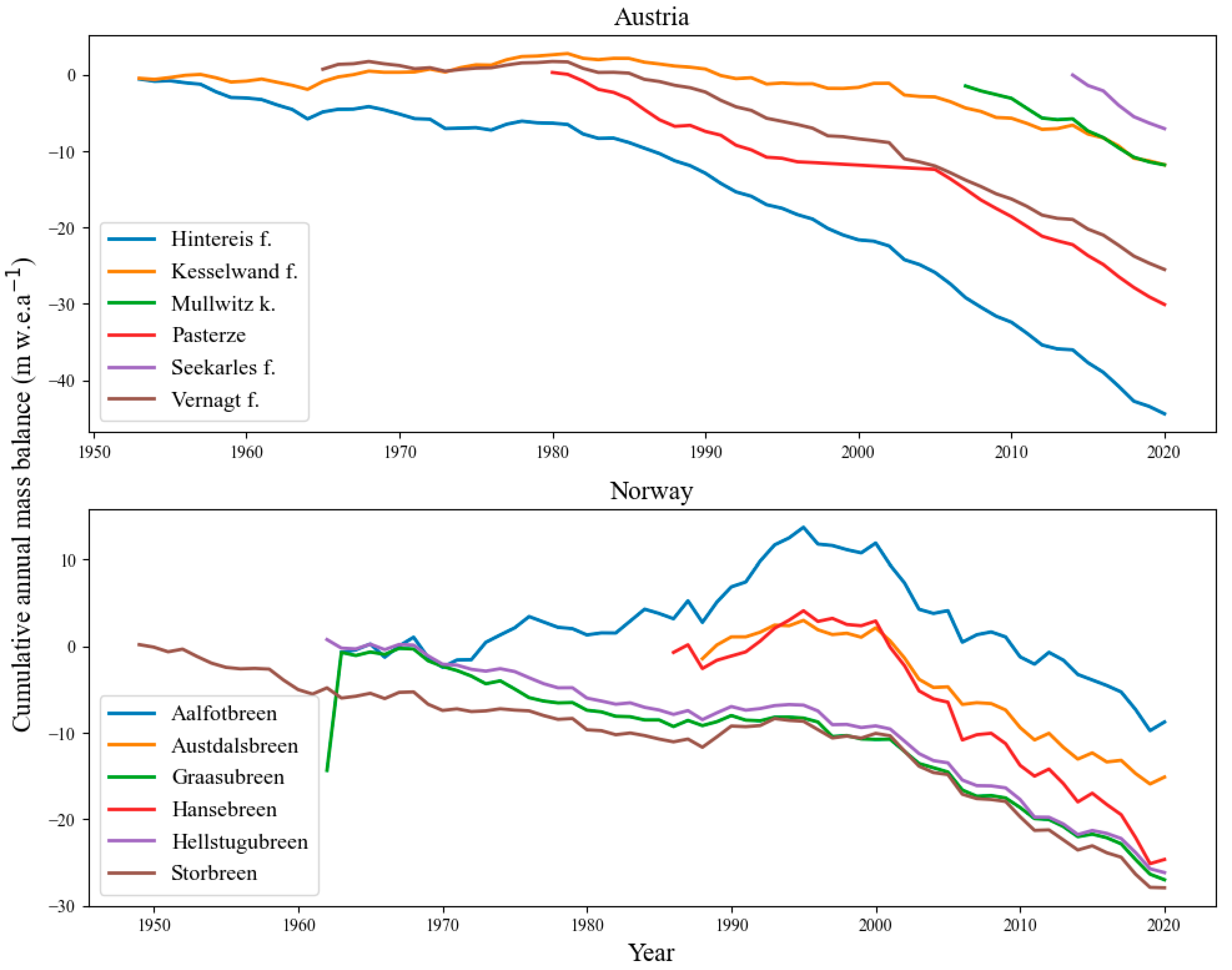
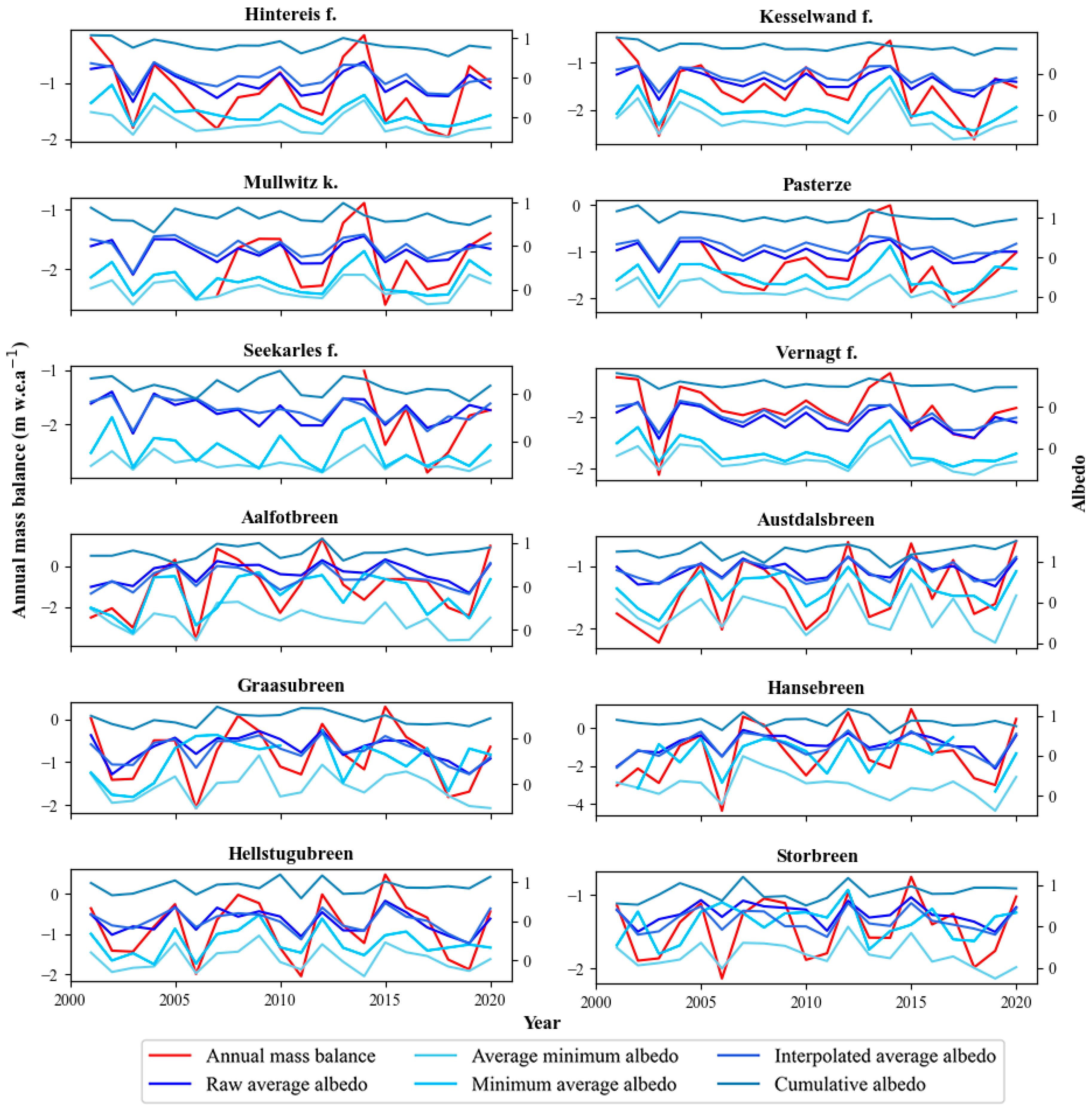
4.1. Time-Series Trends in Mass Balance and Albedo

Figure 3 shows the annual mass balance of glaciers from 2001 to 2020, alongside time variation curves for the raw average albedo, minimum average albedo, average minimum albedo, interpolated average albedo, and cumulative albedo. Over the study period, most glaciers exhibited negative annual mass balance values, indicative of widespread melting, with only a few instances of positive values.

Both raw average and interpolated average methods demonstrated similar patterns, yielding albedo values in the range of 0.3 to 0.6 and an average aggregated albedo of 0.44 across all study areas. Notably, the average minimum and minimum average albedo methods displayed inconsistent patterns in Norwegian and Austrian glaciers. Austrian glaciers, except for Seekarles F, showed similar changing trends in average minimum and minimum average albedo, with respective average values of 0.19 and 0.25. Seekarles F, the glacier with the smallest area and largest annual mass loss, consistently exhibited the lowest albedo value. In Norwegian glaciers, distinct differences in trends were observed, with the average minimum albedo significantly lower (0.26) than the minimum average albedo (0.38). The cumulative albedo, consistently higher than other aggregated albedos, averaged 0.59 across all glaciers. Line graph comparisons indicated that the raw average and interpolated average albedo time series were more consistent with mass balance trends than the average minimum albedo, minimum average albedo, and cumulative albedo time series.

Table 2. Average values of mass balance and albedo, 2001–2010 and 2011–2020.

Name	Annual Mass Balance (m w.e.a.−1/10 Year)		Raw Average Albedo
	2001–2010	2011–2020	2001–2010	2011–2020
Hintereis F	−1.079	−1.200	0.386	0.364
Kesselwand F	−0.404	−0.610	0.470	0.446
Mullwitz K	−0.767	−0.872	0.477	0.459
Pasterze	−1.181	−1.152	0.428	0.418
Seekarles F	/	−1.005	0.340	0.315
Vernagt F	−0.788	−0.924	0.443	0.402
Aalfotbreen	−1.313	−0.753	0.460	0.466
Austdalsbreen	−1.153	−0.573	0.550	0.558
Graasubreen	−0.787	−0.836	0.461	0.429
Hansebreen	−1.669	−1.089	0.454	0.460
Hellstugubreen	−0.851	−0.845	0.410	0.382
Storbreen	−0.964	−0.822	0.470	0.453

presents average mass balance and raw average albedo changes for all glaciers over the two decades (2001–2010 and 2011–2020). From 2001 to 2010, the annual mass balance ranged from −1.669 to −0.404 m w.e.a⁻¹/10 year, averaging −0.996 m w.e.a⁻¹/10 year. Conversely, between 2011 and 2020, the mass balance fluctuated between −1.200 and −0.573 m w.e.a⁻¹/10 year, with an average of −0.890 m w.e.a⁻¹/10 year, indicating a slowdown in the overall mass loss rate during the second decade.

Analyzing mass balance change rates in Austria and Norway revealed a significant increase in the glacier mass balance decline rate in Austria from −0.844 m w.e.a⁻¹/10 year to −0.961 m w.e.a⁻¹/10 year. In contrast, Norwegian glaciers exhibited a reduction in the mass loss rate from −1.123 m w.e.a⁻¹/10 year to −0.820 m w.e.a⁻¹/10 year. Aalfotbreen, Austdalsbreen, and Hansebreen glaciers exhibited the most significant changes, with their average mass balance change rates increasing by 0.560 m w.e.a⁻¹/10 year, 0.580 m w.e.a⁻¹/10 year, and 0.580 m w.e.a⁻¹/10 year, respectively.

Regarding the albedo, observed differences between 2001–2010 and 2011–2020 for all glaciers ranged from 0.006 to 0.041, suggesting minimal changes in MODIS albedo observations during these periods. Austrian and Norwegian glaciers experienced a slight overall albedo decrease, with averages dropping from 0.424 to 0.401 and 0.468 to 0.458, respectively. Similar to mass balance changes, the albedo decrease over the two-decade period was more pronounced in the Austrian region.

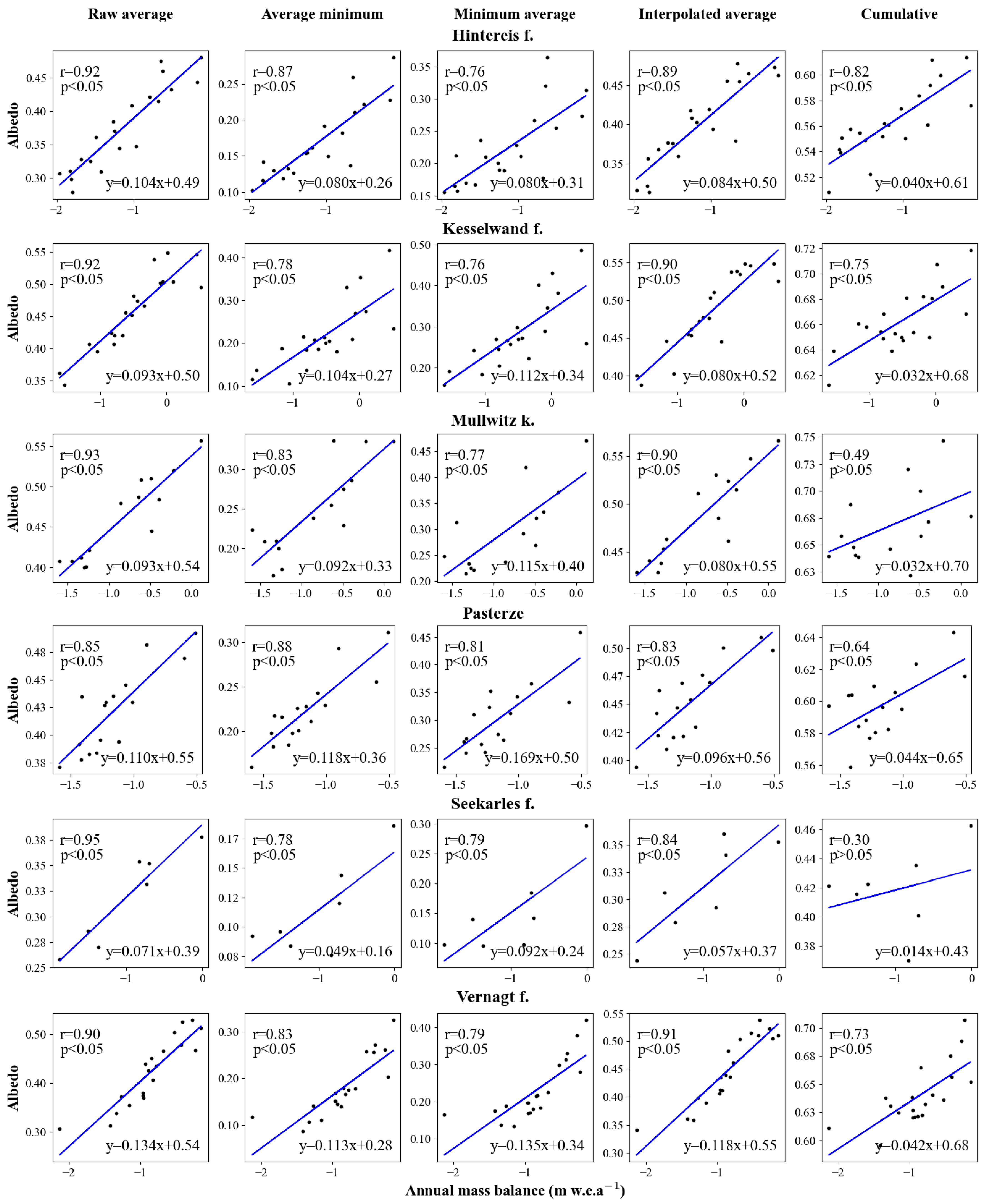
4.2. Annual Mass Balance and Aggregated Albedo Correlation Analysis

Figure 4 and Figure 5 present scatter plots illustrating the relationship between the annual mass balance and the five aggregated albedos for Austrian and Norwegian glaciers, respectively, along with calculated correlation coefficients. The findings reveal varying degrees of correlation across different glaciers.

In all study areas, the raw average albedo demonstrates a substantial correlation with the annual mass balance, ranging from 0.72 to 0.95, with an average correlation coefficient of 0.86. The correlation of interpolated average albedo with the annual mass balance exhibits a similarly high correlation, ranging from 0.83 to 0.93, with an average of 0.89. Furthermore, the minimum average and average minimum aggregation methods display comparable correlation distributions, yielding average values of 0.79 and 0.65, respectively. In contrast, cumulative albedo displays a lower correlation with the annual mass balance, ranging from 0.30 to 0.82, with an average of 0.56.

Summarizing the correlation coefficients of the five aggregated albedos and mass balances for all glaciers in Figure 4 and Figure 5. In Austria, the raw average albedo demonstrates the highest correlation with the annual mass balance, averaging 0.91. Notably, four glaciers (Hintereis F, Kesselwand F, Mullwitz K, and Seekarles F) exhibit r values of no less than 0.92. In the Norwegian region, the interpolated average albedo shows a strong correlation with the annual mass balance, surpassing the correlations of the other four aggregated albedos and the annual mass balance, with an average value of 0.90.

The albedo produced by the minimum average and average minimum methods fails to provide a stable estimate of mass balance, possibly due to cloud cover masking the true values. The cumulative method may be suitable for capturing changes in mass balance for specific glaciers. Consequently, for this study area, the raw average albedo and interpolated average albedo emerge as broadly applicable for estimating glacier mass balance, with the former being particularly suitable for continental glaciers in Austria and the latter for maritime glaciers in Norway.

4.3. Comparison with Other Glacier Mass Balance Inversion Model Indicators

In addition to the albedo, remote sensing observations leverage metrics such as ELA and AAR to estimate the glacier mass balance. The ELA delineates the boundary between the accumulation zone (positive mass balance) and the ablation zone (negative mass balance), representing the altitude of the snowline at the conclusion of the ablation season. The AAR, on the other hand, is the ratio of the accumulation area to the total glacier surface area [11], defining the boundary at which a glacier is in equilibrium with its climatic boundary conditions. Numerous studies have indirectly obtained ELA and AAR data through remote sensing, finding that these indicators are closely related to the glacier mass balance [13,14,15].

In this section, we further examine the correlation between ELA, AAR, and the annual mass balance of the studied glaciers while also comparing the relationship between the raw and interpolated average albedo and the annual mass balance. The findings are presented in

Table 3. Correlation of annual mass balance with different aggregated albedos, ELA and AAR. (Bold text indicates the highest correlation for the same glacier).

Name	Country	Raw Average Albedo	Interpolated Average Albedo	ELA	AAR
Hintereis F	Austria	0.92	0.89	0.86	0.97
Kesselwand F	Austria	0.92	0.90	0.94	0.95
Mullwitz K	Austria	0.93	0.90	0.79	0.76
Pasterze	Austria	0.85	0.83	0.59	0.87
Seekarles F	Austria	0.95	0.84	0.93	0.92
Vernagt F	Austria	0.90	0.91	0.89	0.93
Aalfotbreen	Norway	0.85	0.89	0.80	/
Austdalsbreen	Norway	0.88	0.93	0.92	/
Graasubreen	Norway	0.72	0.89	0.75	/
Hansebreen	Norway	0.85	0.92	0.83	/
Hellstugubreen	Norway	0.83	0.91	0.95	/
Storbreen	Norway	0.77	0.86	0.96	/

. ELA data are sourced from measurements conducted by the WGMS, with availability confirmed, while AAR data are limited to six glaciers in Austria.

The correlation coefficients between the ELA and the annual mass balance in the study area range from 0.75 to 0.96, with an average of 0.85. Specifically, in the Austrian region, the average r value stands at 0.83, while in the Norwegian region, it increases to 0.87. Notably, Norwegian glaciers exhibit a higher correlation between the annual mass balance and ELA. In contrast, the r values for the interpolated average albedo versus the annual mass balance of Norwegian glaciers range from 0.86 to 0.93, with a mean of 0.90, indicating that interpolated average albedo serves as a more precise measure of annual mass balance changes in Norwegian glaciers.

In the Austrian region, the average correlation coefficient for AAR and the annual mass balance is 0.90. Concurrently, the average r-value for the raw average albedo and the annual mass balance across the Austrian region, calculated via the albedo aggregation method, is notably high at 0.91. These findings underscore the reliability of both AAR and the raw average albedo as indicators for estimating changes in glacier mass balance. Upon comparing these two indicators, it is notable that the r value for the raw average albedo and the annual mass balance of the Pasterze glacier is the lowest among the samples, yet it remains substantial at 0.85. Conversely, the r value for AAR and the annual mass balance of the Mullwitz K glacier is comparatively lower, standing at 0.76. Consequently, the raw average albedo emerges as a more stable measure for assessing the annual mass balance.

Synthesizing these findings, it is evident that the ELA, AAR, albedo, and glacier annual mass balance exhibit notable correlations, with the aggregated albedo demonstrating slightly higher correlation coefficients compared to other indicators. These results align with existing studies, which underscore the robust correlation between the albedo and mass balance, arguing that albedo offers more comprehensive insights into glacier surface conditions compared to ELA [52]. Additionally, challenges inherent in the AAR method, such as the difficulty in distinguishing between snow and glacier ice, as well as the fact that cloud cover and terrain shadows affect glacier delineation [53], highlight the advantages of the albedo method, which can achieve equal or superior results while offering a simpler calculation process. It is essential to highlight that the ELA and AAR data utilized in this analysis were derived from field measurements. However, the accuracy of estimated mass balance could potentially be reduced by the inaccuracies inherent in ELA and AAR data inferred from remote sensing observations. Consequently, it can be posited that albedo serves as an excellent indicator for assessing the annual mass balance from remote sensing observations; therefore, it has the potential to predict glacier mass balance trends.

5. Discussion

The results of our study highlight the performance of the raw average and interpolated average methods, which are effective for Austrian and Norwegian glaciers, respectively. It is essential to acknowledge that glaciers in distinct countries may exhibit varying characteristics. In this study, we comprehensively examine the potential factors contributing to these variations, including elevation, cloud cover, precipitation, and temperature.

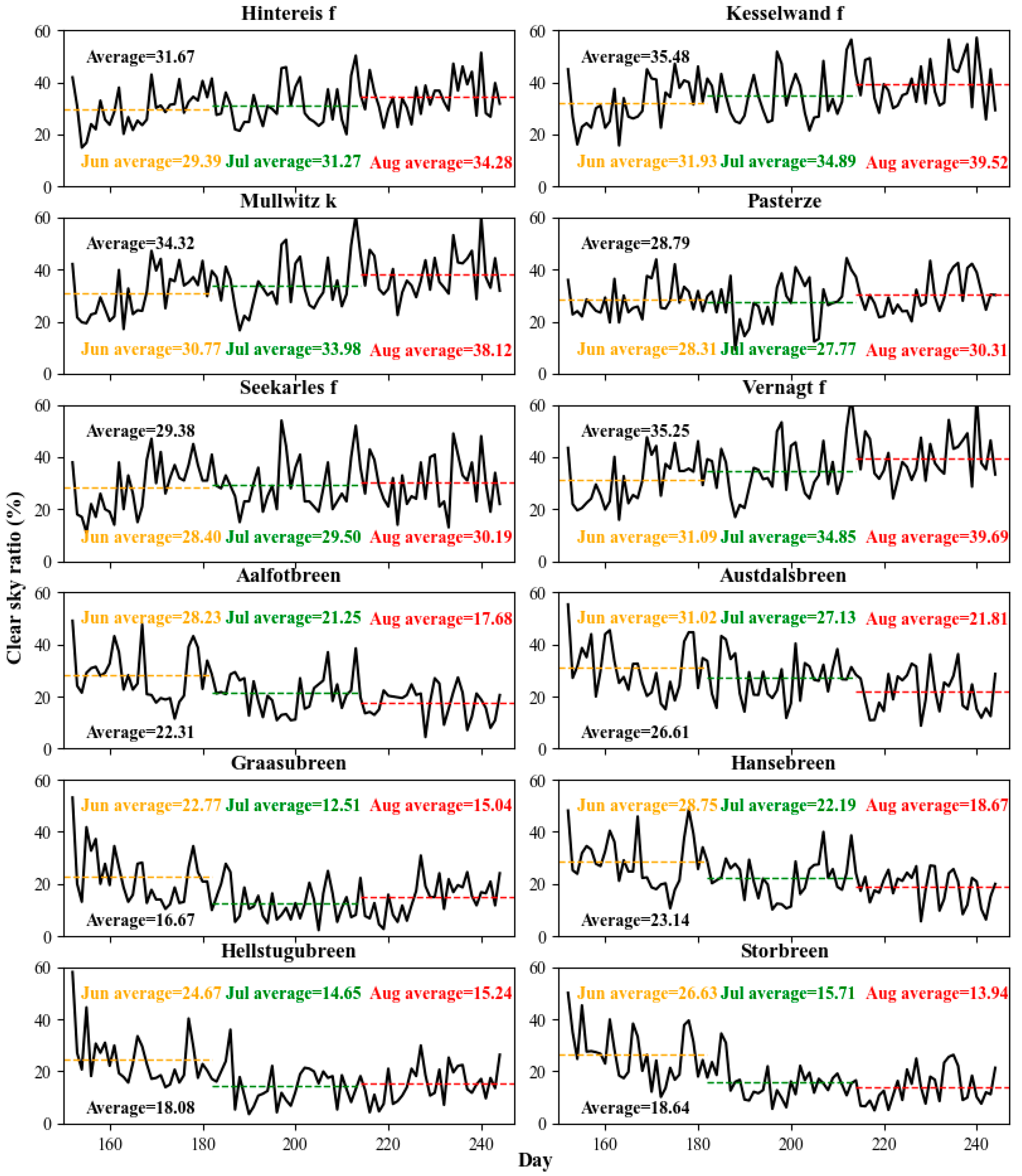
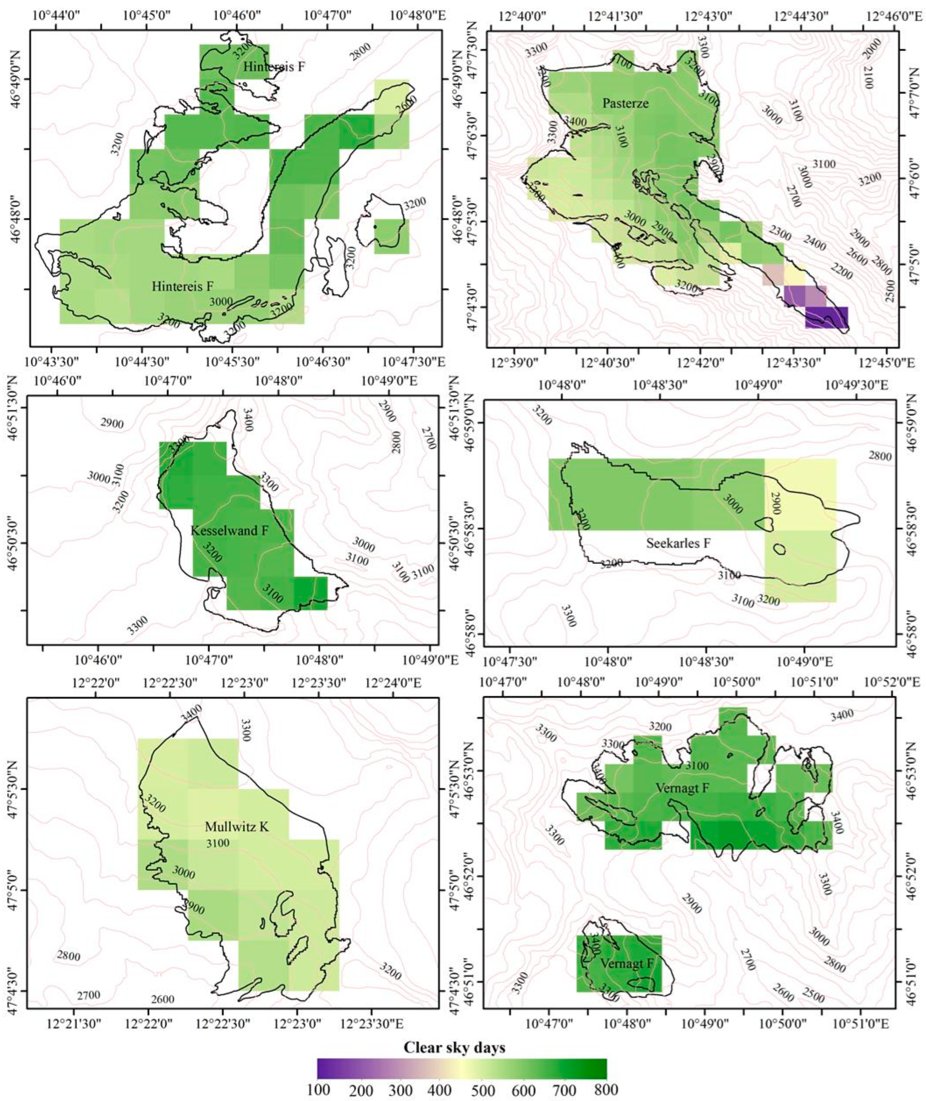
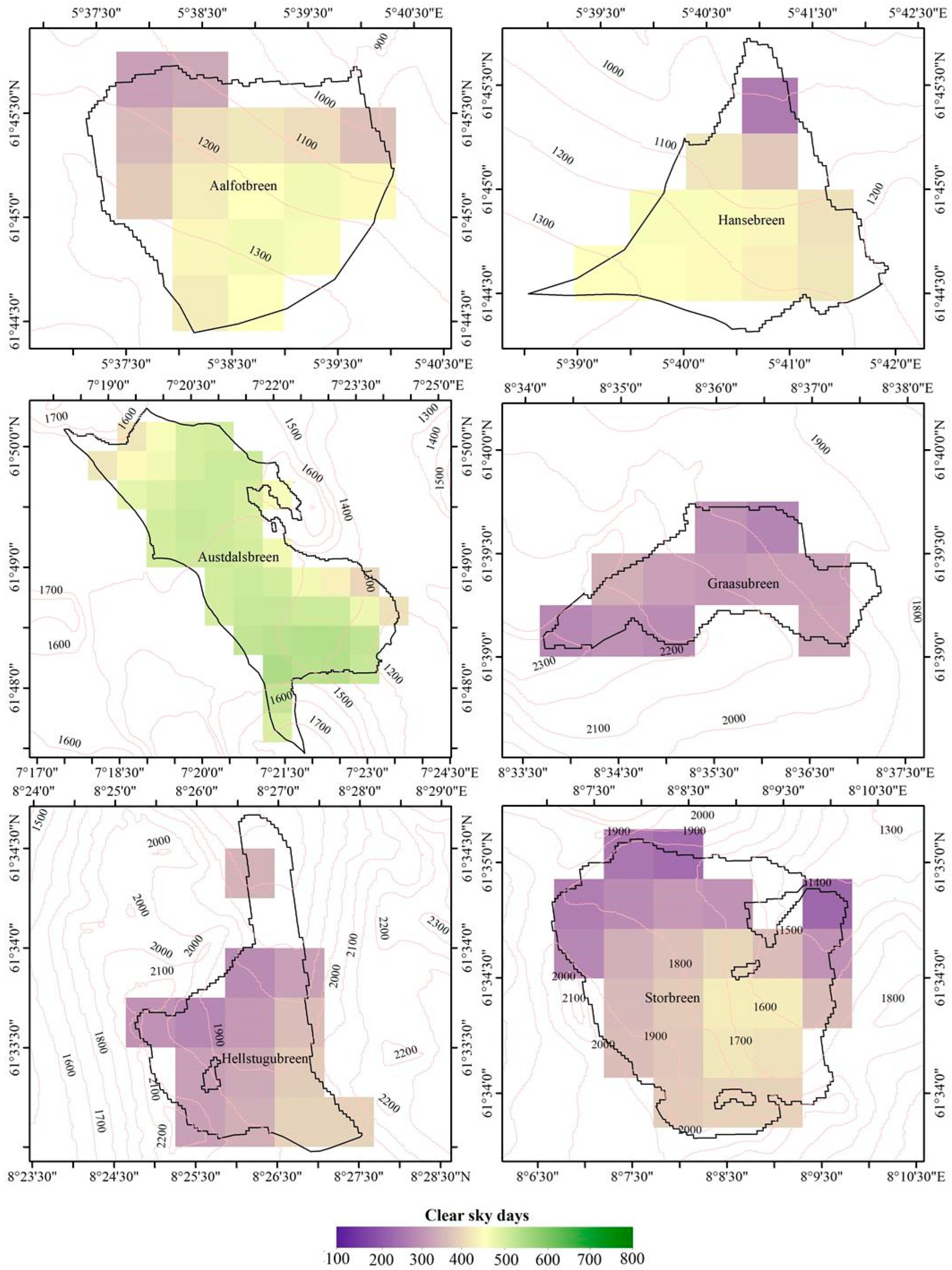
5.1. Effect of Cloud Cover on Different Aggregated Albedo Methods

Figure 6 illustrates the variation in the average daily clear sky rate from June to August for each glacier from 2001 to 2020. The “clear sky rate” refers to the proportion of pixels with effective albedo compared to the total number of pixels of the glacier. It is calculated using the formula: clear sky rate = v/n, where v represents the number of pixels with an effective albedo and n represents the total number of pixels of the glacier. Notably, differences between the Austrian and Norwegian regions emerge. In terms of the average clear sky rate during summer, Austrian glaciers exhibit a significantly higher rate compared to those in the Norwegian region, ranging from 28.79% to 35.25% and 16.67% to 26.61%, respectively, with average values of 32.48% and 20.91%, respectively. Furthermore, the average clear sky rate of Austrian glaciers demonstrates a gradual increase from June to August, while the majority of Norwegian glaciers display a descending trend. The temporal variations in cloud cover over glaciers in these regions manifest distinct patterns influenced by geographical and climatic conditions.

A more in-depth analysis of the spatial distribution of clear sky days in summer for glaciers in Austria and Norway from 2001 to 2020 is presented in Figure 7 and Figure 8. The pixel count of clear sky days for Austrian glaciers ranges from 122 to 713, averaging 577, whereas Norwegian glaciers exhibit a range of 234 to 546 clear sky days, averaging 415. The figure illustrates a clear correlation between elevation and the distribution of clear sky days. Austrian glaciers, with elevations ranging from 2000 m to 3714 m, generally experience more days with clear skies and fewer days with cloud cover. In contrast, Norwegian glaciers, with lower elevations ranging from 890 m to 2277 m, have fewer clear sky days. This elevation-dependent pattern significantly impacts the accuracy of mass balance change estimates in albedo observations, particularly the average minimum albedo. Notably, in maritime glaciers, we observe a stronger linear correlation between the interpolated average albedo and mass balance compared to the minimum average albedo, diverging from previous studies [29]. This divergence may be attributed to the higher cloud cover in Norway, potentially obscuring the true minimum albedo, as supported by our findings in Section 4.2. Here, we report that the correlation between the Norwegian average minimum albedo and the annual mass balance is only 0.52, increasing to 0.78 at higher altitudes. Consequently, the albedo derived from the minimum average and average minimum methods may not offer a stable estimate of mass balance, aligning with previous research [27]. Considering the limited clear sky days in Norway, the raw average method may inadequately reflect glacier ablation, rendering it less precise in measuring changes in glacier mass balance. In contrast, the interpolated average method produces a more accurate estimate of mass balance. To further investigate this, the correlation between the annual mass balance and five aggregated albedos under varying clear sky rates was analyzed. Figure 9 depicts the correlation, revealing that, when the clear sky rate is below 28%, the interpolated average aggregation method yields the highest r value. Conversely, when the clear sky rate exceeds 28%, the raw average aggregation method produces the majority of the highest r values. This underscores the impact of clouds on the relationship between aggregated albedo and the annual mass balance, emphasizing the necessity to consider cloud coverage when selecting an aggregation method for estimating glacier mass balance.

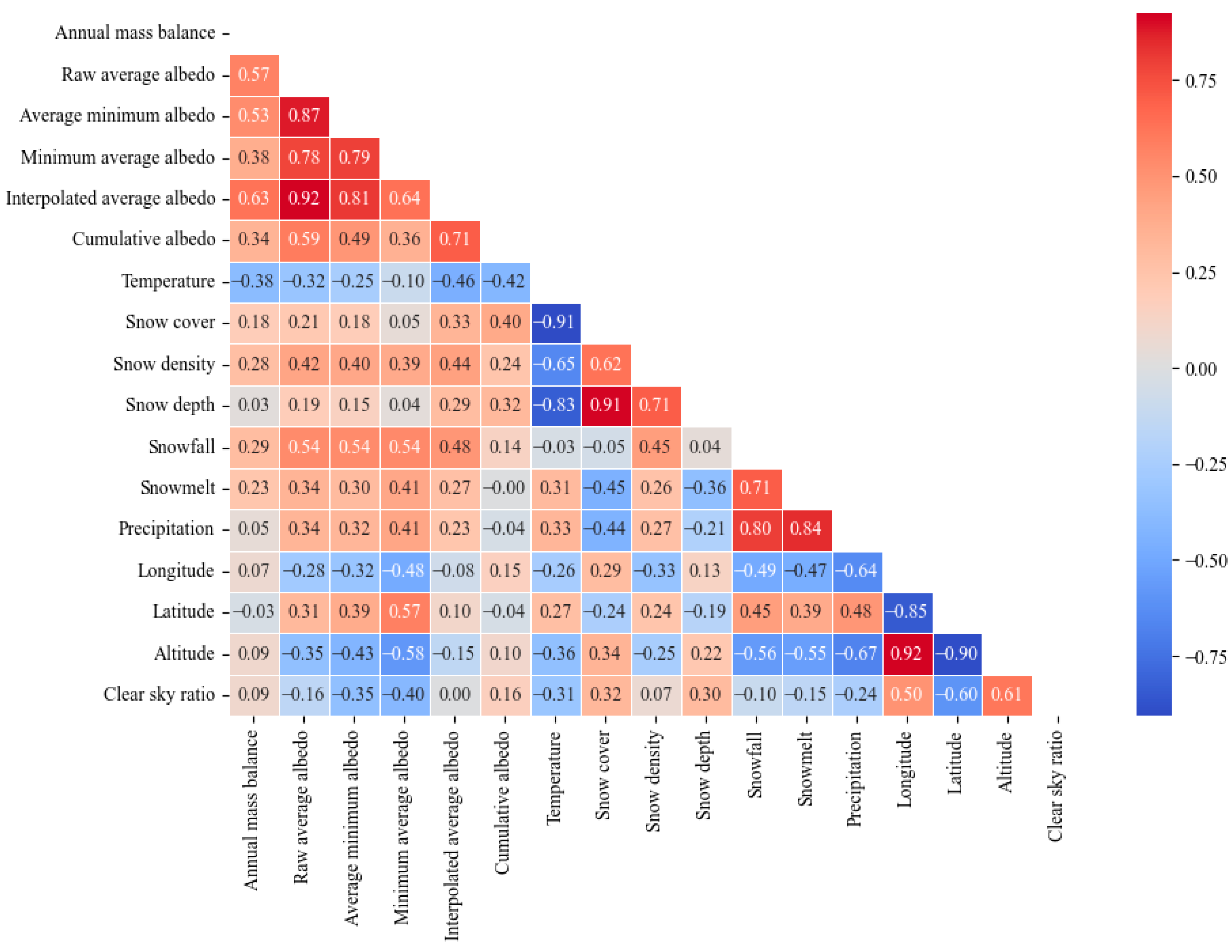
5.2. Effects of Climate Elements on Different Aggregate Albedos

Utilizing ERA5 reanalysis data, which have a spatial resolution of 25 km, we conducted a comprehensive analysis encompassing mass balance, climate elements, and geographical factors. Specifically, we calculated the annual averages of various climate parameters such as snow cover, snow density, snow depth, snowfall, snowmelt, precipitation, and summer temperatures for the studied glaciers. Correlation analyses were then performed between these parameters and the aggregated albedo, longitude, latitude, altitude, and other glacier properties.

Figure 10 reveals significant correlations between the aggregated albedo and the annual mass balance, with the interpolated average albedo showing the highest correlation coefficient (r = 0.63). Additionally, temperature exhibited a negative correlation (−0.38) with the annual mass balance, suggesting that as temperatures decrease, glacier melting intensifies, leading to a reduction in albedo. Furthermore, the aggregated albedo demonstrated a strong positive correlation with snow density and snowfall, highlighting the close relationship between albedo and snow surface conditions. However, the correlations between snowfall, snowmelt, precipitation, and mass balance are relatively weak, suggesting a limited influence on glacier mass balance. Notably, the clear sky rate exhibited significant negative and positive correlations with latitude and altitude, respectively (r = −0.60 and 0.61). This implies that higher latitudes are associated with lower clear sky rates, while higher altitudes are linked to higher clear sky rates. In regions with high clear sky rates, the accuracy of albedo estimates, particularly those obtained through methods like the average minimum albedo and minimum average albedo methods, is expected to be higher.

6. Conclusions

The pursuit of a universally applicable model to quantify the intricate relationship between albedo and glacier mass balance presents a formidable task. This study, focusing on small and medium-sized glaciers in Europe, delves into five distinct albedo aggregation methods for glacier measurement, seeking to elucidate their correlation with mass balance and enhance our comprehension of the albedo-mass balance dynamic. Grounded in a meticulous analysis of the correlation between in situ mass balance measurements and remotely sensed albedo observations, in this research, we study 12 European glaciers from 2001 to 2020.

This investigation underscores the robustness of the raw average and interpolated average methods for glacier mass balance estimations. The raw average albedo exhibits the highest correlation with the annual mass balance of Austrian glaciers, boasting an average correlation coefficient of 0.91. Notably, even in the context of the Seekarles F glacier, with a modest area of 1.04 km², the correlation between the raw average albedo and mass balance reaches an impressive 0.95. Simultaneously, the interpolated average albedo demonstrates a robust correlation with the annual mass balance of Norwegian glaciers, outperforming the other four aggregated albedo methods, with an average correlation coefficient of 0.90.

Cloud cover is a pivotal factor influencing albedo observations, subsequently impacting the efficacy of albedo aggregation methods. Altitude-dependent patterns of clear sky days exert a discernible influence on the accuracy of mass balance changes of albedo observations, underscoring the imperative to account for cloud cover when selecting an aggregation method. The minimum average and average minimum albedo aggregation methods exhibit lower correlations under higher cloud coverage, in stark contrast to the consistently high correlations exhibited by the raw average and interpolated average methods. However, variations arise in the performance of these two methods across glaciers at different altitudes. In high-altitude regions characterized by ample clear sky days, effective albedo observations are sufficient, enabling the use of the raw average albedo for estimating mass balance changes. Conversely, in low-altitude areas where effective albedo observations are scarce, interpolating the average albedo emerges as a more effective approach for mass balance estimations.

The outcomes of this study underscore the potential utility of the raw average and interpolated average albedo for estimating the mass balance of diverse glaciers in the European region. Future investigations could extend these findings in conjunction with other albedo products such as Landsat and Sentinel-2, offering the prospect of combining multiple sources for higher resolution and long-term sequence albedo monitoring alongside MODIS data.

References

1. Qin, D.; Yao, T.; Ding, Y.; Ren, J. (Eds.) Introduction to Cryospheric Science; Springer Nature: Berlin/Heidelberg, Germany, 2021. [Google Scholar] [CrossRef]
2. Huss, M.; Hock, R. Global-scale hydrological response to future glacier mass loss. Nat. Clim. Chang. 2018, 8, 135–140. [Google Scholar] [CrossRef]
3. Bamber, J.L.; Rivera, A. A review of remote sensing methods for glacier mass balance determination. Glob. Planet. Chang. 2007, 59, 138–148. [Google Scholar] [CrossRef]
4. Konz, M.; Seibert, J. On the value of glacier mass balances for hydrological model calibration. J. Hydrol. 2010, 385, 238–246. [Google Scholar] [CrossRef]
5. Machguth, H.; Paul, F.; Hoelzle, M.; Haeberli, W. Distributed glacier mass-balance modelling as an important component of modern multi-level glacier monitoring. Ann. Glaciol. 2006, 43, 335–343. [Google Scholar] [CrossRef]
6. Zemp, M.; Huss, M.; Thibert, E.; Eckert, N.; McNabb, R.W.; Huber, J.; Barandun, M.; Machguth, H.; Nussbaumer, S.U.; Gärtner-Roer, I.; et al. Global glacier mass changes and their contributions to sea-level rise from 1961 to 2016. Nature 2019, 568, 382–386. [Google Scholar] [CrossRef]
7. Brun, F.; Berthier, E.; Wagnon, P.; Kääb, A.; Treichler, D. A spatially resolved estimate of High Mountain Asia glacier mass balances from 2000 to 2016. Nat. Geosci. 2017, 10, 668–673. [Google Scholar] [CrossRef]
8. Wu, K.; Liu, S.; Jiang, Z.; Xu, J.; Wei, J.; Guo, W. Recent glacier mass balance and area changes in the Kangri Karpo Mountains from DEMs and glacier inventories. Cryosphere 2018, 12, 103–121. [Google Scholar] [CrossRef]
9. Liu, L.; Jiang, L.; Jiang, H.; Wang, H.; Ma, N.; Xu, H. Accelerated glacier mass loss (2011–2016) over the Puruogangri ice field in the inner Tibetan Plateau revealed by bistatic InSAR measurements. Remote Sens. Environ. 2019, 231, 111241. [Google Scholar] [CrossRef]
10. Zhou, Y.; Hu, J.; Li, Z.; Li, J.; Zhao, R.; Ding, X. Quantifying glacier mass change and its contribution to lake growths in central Kunlun during 2000–2015 from multi-source remote sensing data. J. Hydrol. 2019, 570, 38–50. [Google Scholar] [CrossRef]
11. Mernild, S.H.; Pelto, M.; Malmros, J.K.; Yde, J.C.; Knudsen, N.T.; Hanna, E. Identification of snow ablation rate, ELA, AAR and net mass balance using transient snowline variations on two Arctic glaciers. J. Glaciol. 2013, 59, 649–659. [Google Scholar] [CrossRef]
12. Pelto, M.; Brown, C. Mass balance loss of Mount Baker, Washington glaciers 1990–2010. Hydrol. Process. 2012, 26, 2601–2607. [Google Scholar] [CrossRef]
13. Tak, S.; Keshari, A.K. Investigating mass balance of Parvati glacier in Himalaya using satellite imagery based model. Sci. Rep. 2020, 10, 12211. [Google Scholar] [CrossRef]
14. Chandrasekharan, A.; Raaj, R.; Pandit, A.; Rabatel, A. Quantification of annual glacier surface mass balance for the Chhota Shigri Glacier, Western Himalayas, India using an Equilibrium-Line Altitude (ELA) based approach. Int. J. Remote Sens. 2018, 39, 9092–9112. [Google Scholar] [CrossRef]
15. Garg, S.; Shukla, A.; Garg, P.K.; Yousuf, B.; Shukla, U.K.; Lotus, S. Revisiting the 24 year (1994–2018) record of glacier mass budget in the Suru sub-basin, western Himalaya: Overall response and controlling factors. Sci. Total Environ. 2021, 800, 149533. [Google Scholar] [CrossRef] [PubMed]
16. Brun, F.; Dumont, M.; Wagnon, P.; Berthier, E.; Azam, M.F.; Shea, J.M.; Sirguey, P.; Rabatel, A.; Ramanathan, A. Seasonal changes in surface albedo of Himalayan glaciers from MODIS data and links with the annual mass balance. Cryosphere 2015, 9, 341–355. [Google Scholar] [CrossRef]
17. Davaze, L.; Rabatel, A.; Arnaud, Y.; Sirguey, P.; Six, D.; Letreguilly, A.; Dumont, M. Monitoring glacier albedo as a proxy to derive summer and annual surface mass balances from optical remote-sensing data. Cryosphere 2018, 12, 271–286. [Google Scholar] [CrossRef]
18. Dumont, M.; Gardelle, J.; Sirguey, P.; Guillot, A.; Six, D.; Rabatel, A.; Arnaud, Y. Linking glacier annual mass balance and glacier albedo retrieved from MODIS data. Cryosphere 2012, 6, 1527–1539. [Google Scholar] [CrossRef]
19. Riihelä, A.; King, M.D.; Anttila, K. The surface albedo of the Greenland Ice Sheet between 1982 and 2015 from the CLARA-A2 dataset and its relationship to the ice sheet’s surface mass balance. Cryosphere 2019, 13, 2597–2614. [Google Scholar] [CrossRef]
20. Negi, H.; Kumar, A.; Kanda, N.; Thakur, N.; Singh, K. Status of glaciers and climate change of East Karakoram in early twenty-first century. Sci. Total Environ. 2021, 753, 141914. [Google Scholar] [CrossRef] [PubMed]
21. Xiao, Y.; Ke, C.; Fan, Y.; Shen, X.; Cai, Y. Estimating glacier mass balance in High Mountain Asia based on Moderate Resolution Imaging Spectroradiometer retrieved surface albedo from 2000 to 2020. Int. J. Clim. 2022, 42, 9931–9949. [Google Scholar] [CrossRef]
22. Helsen, M.M.; van de Wal, R.S.W.; Reerink, T.J.; Bintanja, R.; Madsen, M.S.; Yang, S.; Li, Q.; Zhang, Q. On the importance of the albedo parameterization for the mass balance of the Greenland ice sheet in EC-Earth. Cryosphere 2017, 11, 1949–1965. [Google Scholar] [CrossRef]
23. Cheng, Q.; Hao, W.; Ma, C.; Ye, F.; Luo, J.; Qu, Y. Daily Arctic Sea-Ice Albedo Retrieval with a Multiband Reflectance Iteration Algorithm. IEEE Trans. Geosci. Remote Sens. 2023, 61, 4302712. [Google Scholar] [CrossRef]
24. Ye, F.; Cheng, Q.; Hao, W.; Yu, D.; Ma, C.; Liang, D.; Shen, H. Reconstructing daily snow and ice albedo series for Greenland by coupling spatiotemporal and physics-informed models. Int. J. Appl. Earth Obs. Geoinformation 2023, 124, 103519. [Google Scholar] [CrossRef]
25. Mengyao, L.; Qiang, L.; Ying, Q. A comparative study of long-time series of global-scale albedo products. Int. J. Digit. Earth 2023, 16, 308–322. [Google Scholar] [CrossRef]
26. Greuell, W.; Kohler, J.; Obleitner, F.; Glowacki, P.; Melvold, K.; Bernsen, E.; Oerlemans, J. Assessment of interannual variations in the surface mass balance of 18 Svalbard glaciers from the Moderate Resolution Imaging Spectroradiometer/Terra albedo product. J. Geophys. Res. Atmos. 2007, 112. [Google Scholar] [CrossRef]
27. Williamson, S.N.; Copland, L.; Thomson, L.; Burgess, D. Comparing simple albedo scaling methods for estimating Arctic glacier mass balance. Remote Sens. Environ. 2020, 246, 111858. [Google Scholar] [CrossRef]
28. Di Mauro, B.; Fugazza, D. Pan-Alpine glacier phenology reveals lowering albedo and increase in ablation season length. Remote Sens. Environ. 2022, 279, 113119. [Google Scholar] [CrossRef]
29. Sirguey, P.; Still, H.; Cullen, N.J.; Dumont, M.; Arnaud, Y.; Conway, J.P. Reconstructing the mass balance of Brewster Glacier, New Zealand, using MODIS-derived glacier-wide albedo. Cryosphere 2016, 10, 2465–2484. [Google Scholar] [CrossRef]
30. Dowson, A.J.; Sirguey, P.; Cullen, N.J. Variability in glacier albedo and links to annual mass balance for the gardens of Eden and Allah, Southern Alps, New Zealand. Cryosphere 2020, 14, 3425–3448. [Google Scholar] [CrossRef]
31. Yue, X.; Li, Z.; Wang, F.; Zhao, J.; Li, H.; Bai, C. Spatiotemporal variations in surface albedo during the ablation season and linkages with the annual mass balance on Muz Taw Glacier, Altai Mountains. Int. J. Digit. Earth 2022, 15, 2126–2147. [Google Scholar] [CrossRef]
32. Greuell, W.; Oerlemans, J. Assessment of the surface mass balance along the K-transect (Greenland ice sheet) from satellite-derived albedos. Ann. Glaciol. 2005, 42, 107–117. [Google Scholar] [CrossRef]
33. Zhang, Z.; Jiang, L.; Liu, L.; Sun, Y.; Wang, H. Annual glacier-wide mass balance (2000–2016) of the interior Tibetan Plateau reconstructed from MODIS albedo products. Remote Sens. 2018, 10, 1031. [Google Scholar] [CrossRef]
34. Andreassen, L.; Huss, M.; Melvold, K.; Elvehøy, H.; Winsvold, S. Ice thickness measurements and volume estimates for glaciers in Norway. J. Glaciol. 2014, 61, 763–775. [Google Scholar] [CrossRef]
35. Huss, M.; Farinotti, D. Distributed ice thickness and volume of all glaciers around the globe. J. Geophys. Res. Earth Surf. 2012, 117. [Google Scholar] [CrossRef]
36. Mannerfelt, E.S.; Dehecq, A.; Hugonnet, R.; Hodel, E.; Huss, M.; Bauder, A.; Farinotti, D. Halving of Swiss glacier volume since 1931 observed from terrestrial image photogrammetry. Cryosphere 2022, 16, 3249–3268. [Google Scholar] [CrossRef]
37. Beniston, M.; Farinotti, D.; Stoffel, M.; Andreassen, L.M.; Coppola, E.; Eckert, N.; Fantini, A.; Giacona, F.; Hauck, C.; Huss, M.; et al. The European mountain cryosphere: A review of its current state, trends, and future challenges. Cryosphere 2018, 12, 759–794. [Google Scholar] [CrossRef]
38. Réveillet, M.; Vincent, C.; Six, D.; Rabatel, A. Which empirical model is best suited to simulate glacier mass balances? J. Glaciol. 2017, 63, 39–54. [Google Scholar] [CrossRef]
39. Thibert, E.; Eckert, N.; Vincent, C. Climatic drivers of seasonal glacier mass balances: An analysis of 6 decades at Glacier de Sarennes (French Alps). Cryosphere 2013, 7, 47–66. [Google Scholar] [CrossRef]
40. Huss, M.; Dhulst, L.; Bauder, A. New long-term mass-balance series for the Swiss Alps. J. Glaciol. 2015, 61, 551–562. [Google Scholar] [CrossRef]
41. Abermann, J.; Kuhn, M.; Fischer, A. Climatic controls of glacier distribution and glacier changes in Austria. Ann. Glaciol. 2011, 52, 83–90. [Google Scholar] [CrossRef]
42. Engelhardt, M.; Schuler, T.V.; Andreassen, L.M. Sensitivities of glacier mass balance and runoff to climate perturbations in Norway. Ann. Glaciol. 2015, 56, 79–88. [Google Scholar] [CrossRef]
43. Leigh, J.R.; Stokes, C.R.; Evans, D.J.A.; Carr, R.J.; Andreassen, L.M. Timing of Little Ice Age maxima and subsequent glacier retreat in northern Troms and western Finnmark, northern Norway. Arct. Antarct. Alp. Res. 2020, 52, 281–311. [Google Scholar] [CrossRef]
44. Riggs, G.A.; Hall, D.K.; Román, M.O. MODIS Snow Products Collection 6 User Guide; National Snow and Ice Data Center: Boulder, CO, USA, 2015. [Google Scholar]
45. Williamson, S.N.; Copland, L.; Hik, D.S. The accuracy of satellite-derived albedo for northern alpine and glaciated land covers. Polar Sci. 2016, 10, 262–269. [Google Scholar] [CrossRef]
46. Gunnarsson, A.; Gardarsson, S.M.; Pálsson, F.; Jóhannesson, T.; Sveinsson, G.B. Annual and inter-annual variability and trends of albedo of Icelandic glaciers. Cryosphere 2021, 15, 547–570. [Google Scholar] [CrossRef]
47. Kaufmann, V.; Ploesch, R. Mapping and visualization of the retreat of two cirque glaciers in the Austrian Hohe Tauern National Park. Int. Arch. Photogramm. Remote Sens. 2000, 33, 446–453. [Google Scholar]
48. Yue, X.; Zhao, J.; Li, Z.; Zhang, M.; Fan, J.; Wang, L.; Wang, P. Spatial and temporal variations of the surface albedo and other factors influencing Urumqi Glacier No. 1 in Tien Shan, China. J. Glaciol. 2017, 63, 899–911. [Google Scholar] [CrossRef]
49. Olson, M.; Rupper, S. Impacts of topographic shading on direct solar radiation for valley glaciers in complex topography. Cryosphere 2019, 13, 29–40. [Google Scholar] [CrossRef]
50. Stillinger, T.; Roberts, D.A.; Collar, N.M.; Dozier, J. Cloud masking for Landsat 8 and MODIS Terra over snow-covered terrain: Error analysis and spectral similarity between snow and cloud. Water Resour. Res. 2019, 55, 6169–6184. [Google Scholar] [CrossRef] [PubMed]
51. Cuffey, K.M.; Paterson, W.S.B. The Physics of Glaciers; Academic Press: Cambridge, MA, USA, 2010. [Google Scholar]
52. Hu, Z.; Kuenzer, C.; Dietz, A.J.; Dech, S. The potential of Earth observation for the analysis of cold region land surface dynamics in europe—A review. Remote Sens. 2017, 9, 1067. [Google Scholar] [CrossRef]
53. Rastner, P.; Prinz, R.; Notarnicola, C.; Nicholson, L.; Sailer, R.; Schwaizer, G.; Paul, F. On the automated mapping of snow cover on glaciers and calculation of snow line altitudes from multi-temporal landsat data. Remote Sens. 2019, 11, 1410. [Google Scholar] [CrossRef]
Figure 1. Study area showing the glaciers studied in this paper: (a) Austria, and (b) Norway. See Table 1 for location details.
Remotesensing 16 01914 g001
Figure 2. Measured cumulative annual mass balance changes in the study area.
Remotesensing 16 01914 g002
Figure 3. Time-series changes in annual mass balance and five aggregated albedos.
Remotesensing 16 01914 g003
Figure 4. Regression between five aggregated albedos and annual mass balance for Austrian glaciers.
Remotesensing 16 01914 g004
Figure 5. Regression between five aggregated albedos and annual mass balance for Norwegian glaciers.
Remotesensing 16 01914 g005
Figure 6. Temporal changes in the glacier summer clear sky ratio from 2001 to 2020.
Remotesensing 16 01914 g006
Figure 7. Spatial distribution of summer clear sky days in Austrian glaciers from 2001 to 2020.
Remotesensing 16 01914 g007
Figure 8. Spatial distribution of summer clear sky days in Norwegian glaciers from 2001 to 2020.
Remotesensing 16 01914 g008
Figure 9. Correlation distribution between five aggregated albedos and annual mass balance under different clear sky rates.
Remotesensing 16 01914 g009
Figure 10. Correlation distribution between different elements.
Remotesensing 16 01914 g010