Abstract
Coastal areas are among the most productive areas in the world, ecologically as well as economically. Sea Surface Temperature (SST) has evolved as the major essential climate variable (ECV) and ocean variable (EOV) to monitor land–ocean interactions and oceanic warming trends. SST monitoring can be achieved by means of remote sensing. The current relatively coarse spatial resolution of established SST products limits their potential in small-scale, coastal zones. This study presents the first analysis of the TIMELINE 1 km SST product from AVHRR in four key European regions: The Northern and Baltic Sea, the Adriatic Sea, the Aegean Sea, and the Balearic Sea. The analysis of monthly anomaly trends showed high positive SST trends in all study areas, exceeding the global average SST warming. Seasonal variations reveal peak warming during the spring, early summer, and early autumn, suggesting a potential seasonal shift. The spatial analysis of the monthly anomaly trends revealed significantly higher trends at near-coast areas, which were especially distinct in the Mediterranean study areas. The clearest pattern was visible in the Adriatic Sea in March and May, where the SST trends at the coast were twice as high as that observed at a 40 km distance to the coast. To validate our findings, we compared the TIMELINE monthly anomaly time series with monthly anomalies derived from the Level 4 CCI SST anomaly product. The comparison showed an overall good accordance with correlation coefficients of R > 0.82 for the Mediterranean study areas and R = 0.77 for the North and Baltic Seas. This study highlights the potential of AVHRR Local Area Coverage (LAC) data with 1 km spatial resolution for mapping long-term SST trends in areas with high spatial SST variability, such as coastal regions.
1. Introduction
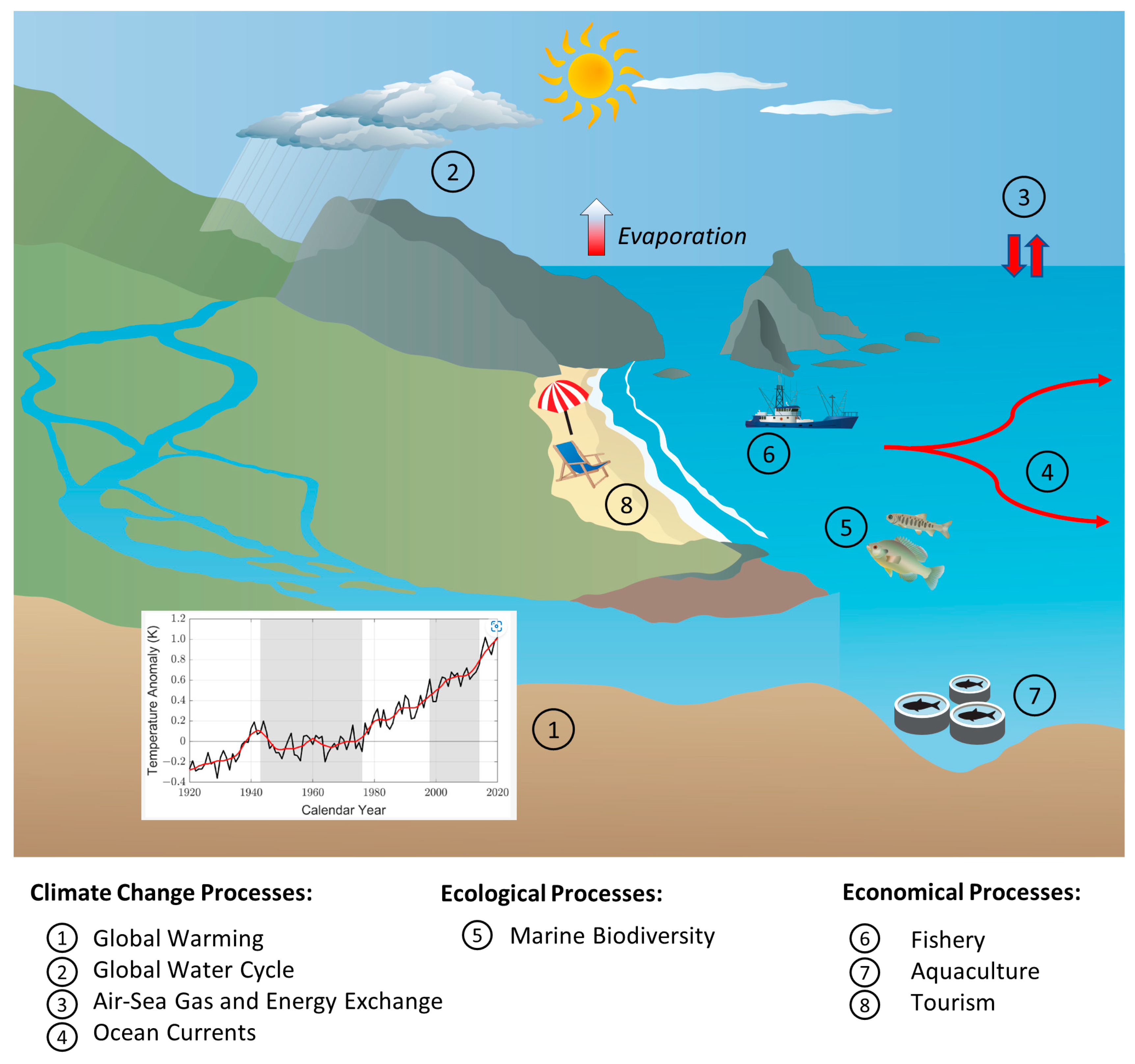
Sea Surface Temperature (SST) is a key essential climate variable (ECV) [1] as well as an essential ocean variable (EOC) [2] describing the temperature of the uppermost ocean layer. In the context of remote sensing, SST is mostly considered as the skin temperature of the ocean, which can be derived from thermal infrared radiation. Besides air temperature, SST is one of the main indicators of climate change [3]. It plays an important role in global lateral energy transport, radiative and turbulent air–sea energy exchange, absorption of anthropogenic greenhouse gases in the ocean, modification of the atmospheric boundary layer, and the global water cycle [4]. Furthermore, changes in SST affect marine ecosystems [5] and also have economic impacts, e.g., on the fishery [6] and aquaculture industries [7] and on tourism [8]. Therefore, they need to be monitored closely. Figure 1 provides an overview of global change processes, which can be derived from SST. After the Copernicus program of the European Union reported record-breaking marine heat-waves for summer 2023 [9], SST was in the headlines across all media. However, the years before this were already setting global temperature records again and again, which is reflected by the fact that the ten warmest years on record occurred after 2009 [10].

Figure 1.
Overview figure illustrating global change processes affected by SST changes.
Satellite observations have become a standard in monitoring SST and a range of sensors are used in this context. The Advanced Very-High-Resolution Radiometer (AVHRR) and Landsat provide the longest time series starting from the early 1980s. Meanwhile, AVHRR provides high temporal resolution (several times daily) and medium spatial resolution (1 km to 4 km), while Landsat provides high spatial resolution (60 m to 100 m) but only low temporal resolution (16 days). Often-employed sensors with shorter time series include the Moderate-Resolution Imaging Spectroradiometer (MODIS), operating since the year 2000, the Along-Track Scanning Radiometer (ATSR), operating between 1991 and 2011, and its successor the Advanced Along-Track Scanning Radiometer (AATSR), operating between 2002 and 2012. Satellite-based SST research has led to a number of SST products which are used by the scientific community. The National Aeronautics and Space Administration (NASA), for example, published a 4 km resolution daytime SST product derived from MODIS Aqua data [11]. Another SST product was developed from 4 km resolution AVHRR data within the pathfinder project [12]. Recently, the most established long-term SST data record was published within the Climate Change Initiative (CCI) by the European Space Agency (ESA), which utilized 4 km AVHRR data and ASTR data to create a global harmonized SST for the period 1980 to 2016 with 0.05° spatial resolution [13].
Currently, a new long-term SST product has been developed in the framework of the TIMELINE (Time Series Processing of Medium-Resolution Earth Observation Data assessing Long-Term Dynamics In our Natural Environment) project. The TIMELINE project conducted at the German Remote Sensing Data Center (DFD) of the German Aerospace Center (DLR) aims to generate well-calibrated and harmonized time series spanning four decades from the early 1980s based on 1 km Local Area Coverage (LAC) AVHRR data over Europe, which are exclusively received and archived at the DLR. Besides SST, the TIMELINE product suite includes LST, NDVI, Hot Spot/Burnt Area, Cloud Probability, and Snow Cover [14]. First analyses of the higher-level (Level 3) products are on the way, and the products are to be released on the DLR Geoservice (https://geoservice.dlr.de/web/) in the near future. A recently published study analyzing the TIMELINE NDVI product revealed unique insights into long-term seasonal vegetation dynamics across Europe [15]. The TIMELINE Level 3 SST product contains daily, 10-day, and monthly composites of SST including the corresponding statistics like mean, standard deviation, and uncertainty of the SST product.
Many studies were conducted on regionally and globally increasing SST. Far less attention has been given to SST trends in coastal areas [16]. During the last three decades, more than 70% of the world’s coastal areas experienced significant increases in SST at a mean rate of 0.25 °C/decade. Still, warming rates are highly heterogeneous, both spatially and seasonally [17]. These regions underly many local and remote forcing factors like wind direction, cloudiness, ocean currents, thermocline depth, and upwelling intensity [18]. While upwelling can buffer the effects of global warming nearshore [19], many coastal areas experience higher warming rates than open waters [16]. Little attention has been given to SST trends in coastal areas, and regional variations and changes in the seasonality are yet not fully understood [16]. Also, the authors of [17] emphasize the need for high-spatial-resolution studies to close this gap. This reflects the relevance of long-term SST trend studies with high spatial resolution.
This research gap can be filled with the new TIMELINE SST product. In this study, we present the first analysis of TIMELINE SST anomalies for the years 1990–2022. To our knowledge, to date, there is no other dataset which allows the observation of trends and patterns of more than 30 years of SST at a 1 km resolution. We have chosen four example regions, in which we expect high spatial variability of trends, because of their high proportion of nearshore areas. Furthermore, these regions have a high economic and ecological relevance. The regions are namely the North and Baltic Seas, the Adriatic Sea, the Aegean Sea, and the Balearic Sea. These regions are based on several sub-basins defined by the International Hydrographic Organization (IHO). The following steps are carried out:
- Analyze the SST anomaly time series.
- Compare the TIMELINE SST anomalies to SST anomalies from the ESA CCI product.
- Interpret the spatial distribution of monthly SST anomaly trends with a special focus on their distance to the coastline.
- Contrast the results with findings of previous SST studies and discuss the advantages and disadvantages of the TIMELINE SST product.
2. Data and Study Areas
2.1. Data
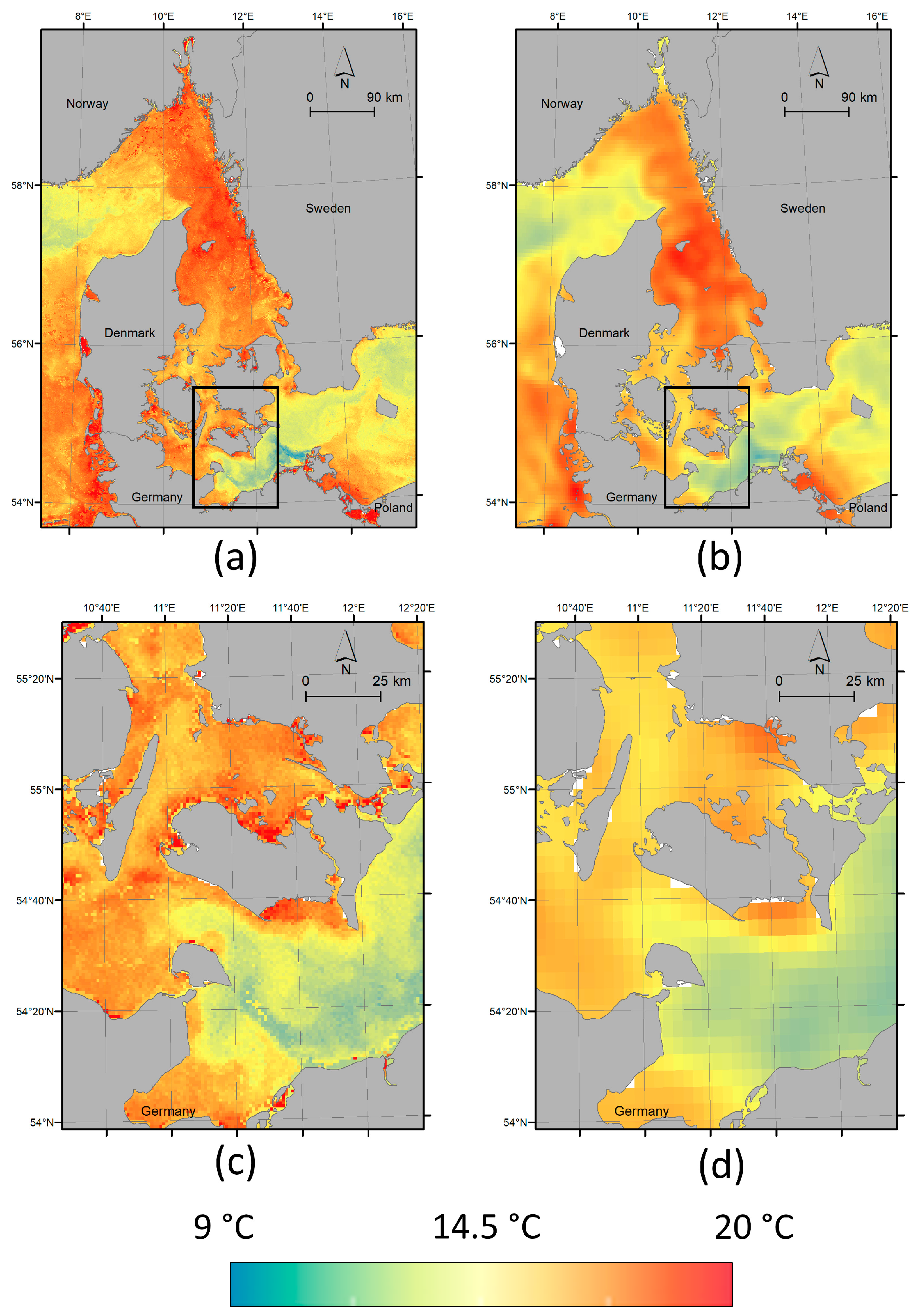
We have employed two data sources in this study. For the analysis of the SST anomalies and anomaly trends of the European coastal zones, we used the Level 3 10-day TIMELINE SST product. For validation and comparison of the results, the Level 4 daily CCI SST anomaly product was employed. Both datasets are described in the following. The different spatial resolutions of the TIMELINE SST and CCI SST are displayed in Figure 2.
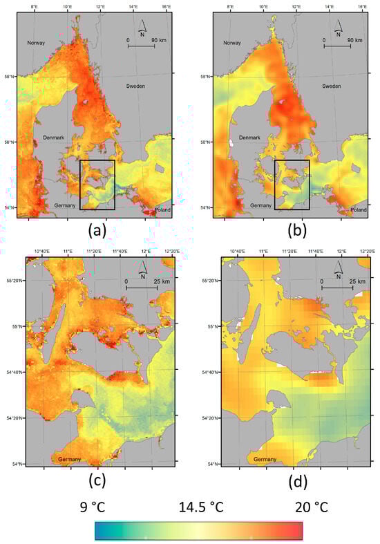
Figure 2.
Example for TIMELINE daily Level 3 (a,c) and CCI daily Level 4 (b,d) SSTs on 7 June 2007 displaying the different spatial resolutions of these products. The black rectangles in (a,b) represent extend of the zoomed-in areas in (c,d).
2.1.1. TIMELINE SST
The TIMELINE SST product was derived from brightness temperatures of the AVHRR channels 4 and 5. Atmospheric correction was performed with an extension of the Split Window Algorithm by [20]. This algorithm was extended by [21] with coefficients to account for the influence of water vapor (TCWV), view angle (VA), and temperature range whilst harmonizing the AVHRR sensors. Emissivity values of ε = 0.991 for channel 4 and ε = 0.985 for channel 5 were taken from [22]. Clouds were masked using the TIMELINE Apollo cloud product [23]. Level 2 SST was validated with shipborne radiometer measurements derived in the framework of the Ships4SST project [24] and buoy measurements from the NOAA Global Drifter Array [25] during the development of the product [14,26]. Furthermore, prior to this study, we conducted a validation study of the TIMELINE SST, including a direct comparison between TIMELINE SST and the well-validated CCI Level 4 SST product [18]. The results of this validation study are presented in the Supplementary Material (Figures S1–S3). Figure S1 shows the results of the validation of TIMELINE SST with SSTs from 195 drifting buoys for the years 2007–2013. The comparison resulted in 5484 data points, showing a high accordance with an R2 of 0.97, a mean absolute difference (MAD) of 0.89 °C, and a bias of 0.01 °C. Figure S2 shows the difference between the TIMELINE and CCI monthly maximum SST for the North Sea and the Baltic Sea for the years 1990–2016, revealing a slightly higher standard deviation of the difference for the period 1990–2002. The comparison showed an overall MAD of 0.77 °C for the North Sea and 0.89 °C for the Baltic Sea and a bias of −0.12 °C for the North Sea and −0.15 °C for the Baltic Sea. Figure S3 shows the difference between TIMELINE and CCI SST for three 10-day maximum SST composites in summer and winter. The differences were classified for classes of TCWV and VA, which are the main drivers of uncertainty during the atmospheric correction. The results show a stable difference for all TCWV classes if the VA is smaller than 50°.
While the Level 2 product contains SST in orbit projection, the Level 3 product includes daily, 10-day, and monthly statistics of SST in map projection (Lambert Azimuthal Equal Area (LAEA) with ETRS89 datum) with a 1 km resolution. These statistics imply the minimum, maximum, median, and mean SST for the respective period. Only high-quality SST observations are used for the compositing, which is ensured by filtering out observations acquired with a sensor view angle higher than 50° and a standard-deviation-based filter for the respective period. In this study, the medium SSTs from the 10-day Level 3 products are used. To apply the Split Window Algorithm for atmospheric correction, two thermal bands are necessary. Therefore, data from AVHRR/1 (NOAA-6, 8 and 10) were not used in this study. Table 1 provides an overview of which platforms and sensors have been utilized for which part of the time series. In total, 5072 10-day products were processed, which comprise a data volume of 483.6 GB.

Table 1.
Overview of employed platforms and sensors and their respective period.
2.1.2. CCI SST
The CCI SST products combine observations derived from AVHRR and ATSR between 1980 and 2022. Atmospheric correction methods are different for the two sensors: While for ATSR, the dual-view brightness temperatures can be used for the correction, for AVHRR, an atmospherically smoothed maximum likelihood approach is used [13]. AVHRR brightness temperatures are harmonized beforehand by matching up simultaneously acquired observations between the different AVHRR sensors. Analogous to the TIMELINE products, the CCI Level 2 products contain instantaneous SST in orbit projection. Observations for one day are composited and gridded for each sensor to obtain daily Level 3 products with 0.05° resolution. Based on them, the data from AVHRR and ATSR are merged and interpolated to calculate the gap-free daily Level 4 SST analysis products [13]. The CCI processing scheme includes a probabilistic cloud detection, a sea ice mask, an adjustment for daytime, and an adjustment to represent SST at 20 cm depth. A median uncertainty for pixel SSTs of 0.18 °C is stated [13]. Based on the Level 4 product, the project also delivered daily SST anomalies for the period between 1980 and 2016 [27], which represent the daily deviation of SST from the climatological mean of this period for the respective day. This product, which can be freely downloaded from the catalogue of the Centre for Environmental Analysis (CEDA), was used as a reference in this study.
2.2. Study Regions
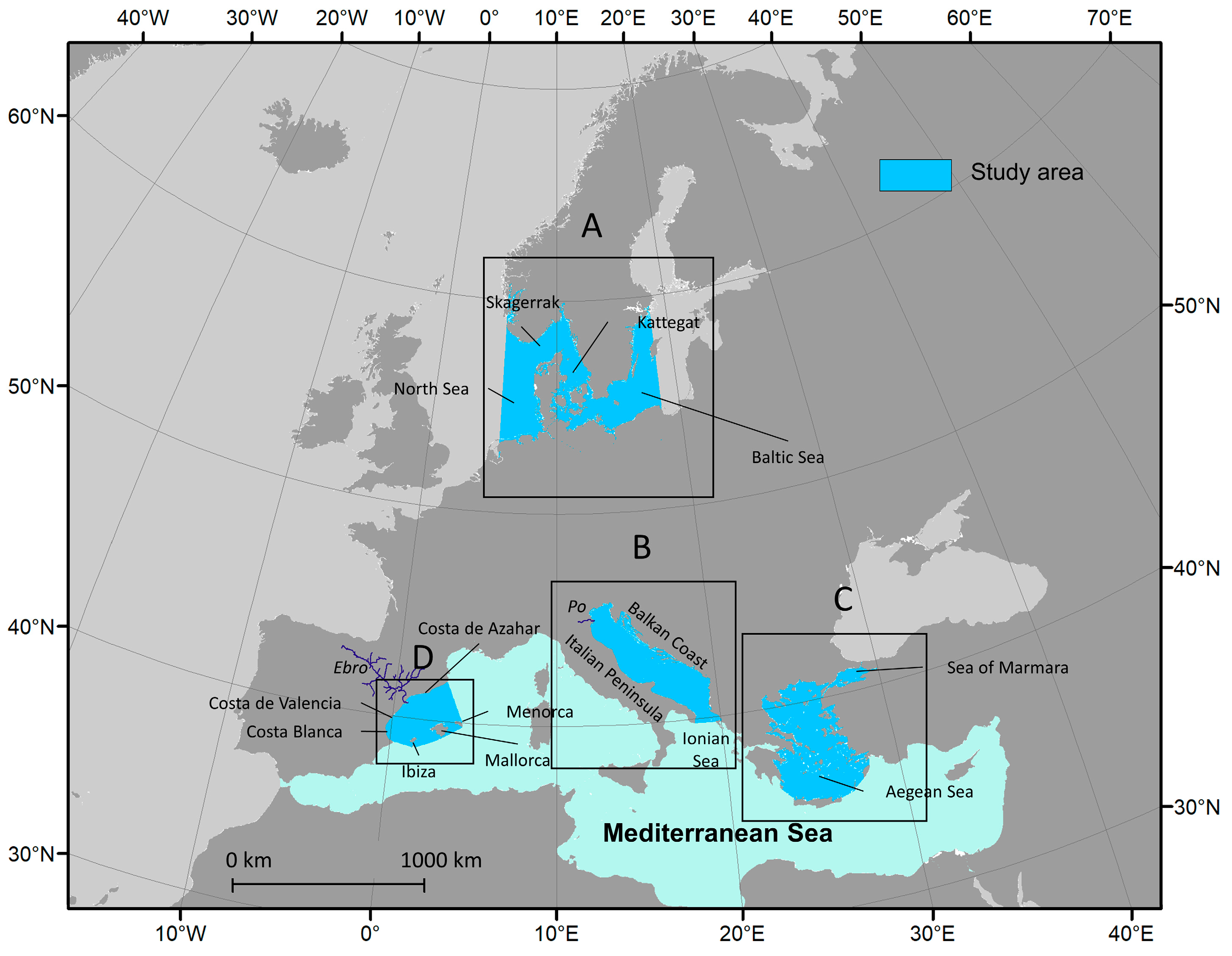
The TIMELINE Level 3 products which cover Europe and Northern Africa have the same extent as the European Environmental Agency (EEA) reference grid: 900,000 m west and 900,000 m south to 7,400,000 m east and 5,500,000 m north. For this study, four regions of special interest were selected, which are characterized by a high proportion of nearshore areas with high economic and ecological relevance. The regions are based on the sub-basins defined by the IHO and are displayed in Figure 3. The regions are, namely, the North and Baltic Seas also including the IHO basins Skagerrak and Kattegat, the Adriatic Sea, the Aegean Sea including the IHO basin with the same name, the Sea of Marmara, and the Balearic Sea. SST trends in these regions have already been subject to previous studies for which an overview is given in Table 2. Study regions are described below in further detail.
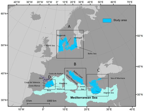
Figure 3.
Overview of the study areas: North and Baltic Seas (A), Adriatic Sea (B), Aegean Sea (C), and Balearic Sea (D). The rectangles highlight the study areas, the light blue color highlights the extent of the Mediterranean Sea.
Table 2.
Recent SST time series trend analysis conducted for our study regions.
2.2.1. North and Baltic Seas
For this study, the North and Baltic Seas were analyzed within the bounding box of x-minimum = 5.5°E, x-maximum = 18.5°E, y-minimum = 52.5°N and y-maximum = 62.5°N. While the North Sea has a direct connection to the Atlantic Ocean, the Baltic Sea is a semi-enclosed ocean in northern Europe and the second largest brackish sea after the Black Sea. It has a low average depth (~54 m) and a strongly variable bathymetry, which limits the exchange between sub-basins [31]. Kattegat and Skagerrak form a strait that connects the North Sea with the Baltic Sea. The area is one of the busiest shipping routes in the world. The Danish and the German Baltic and North Sea coasts are important tourist areas. The Baltic Sea experiences one of the strongest increases in SST observed in a large marine ecosystem [32]. SST trends display a strong seasonal variability and differ among the different sub-basins. Intense warming in the western and eastern part of the Baltic proper could be related to changes in surface winds, yielding a decrease in the upwelling frequencies along the Swedish coast and an increase in heat flux in the eastern Baltic proper [31]. Furthermore, the Baltic Sea is threatened by anthropogenically induced hypoxia and eutrophication. While hypoxia is mainly caused by river-borne nutrient loads and atmospheric deposition, the contribution of increasing SSTs cannot be ruled out [33].
2.2.2. Adriatic Sea
The Adriatic Sea separates the Italian Peninsula from the Balkans. The northern and central parts are shelf areas with a depth of less than 100 m. In the southern part, the Adriatic Sea is in exchange with the Ionian Sea. The climate is influenced by the Bora wind, which is known to be associated with cold and dry continental air [34]. The physicochemical processes are directly influenced by the inflow of water from the river Po in the north as well as its specific topography [35]. The Adriatic Sea has a lower salinity level than the rest of the Mediterranean due to the inflow of inland waters, which contain about a third of the freshwater that enters the entire Mediterranean Sea [35]. The eastern Balkan coast experienced a substantial warming of 1 °C between 1979 and 2015 [36].
2.2.3. Aegean Sea
The Aegean Sea is located between the Balkan Peninsula and Anatolia and is connected to the Sea of Marmara by the Dardanelles. Most of the Greek Islands are located in this area. The area belongs to the top tourist destinations in Europe, and the tourism in the Aegean Sea accounts for a large proportion of the Greek economy. According to the IPCC reports, this region is considered to be one of the regions most vulnerable to climate change. SST trends in the Aegean Basin are significantly higher (0.38 °C/decade, 0.6 °C/decade when considering the years 2003–2019) than the trends of the whole Mediterranean Sea (0.35 °C/decade) [28,37].
2.2.4. Balearic Sea
The Balearic Sea is located in the northwestern Mediterranean Sea between the Balearic Islands (Ibiza, Mallorca, and Menorca) and the eastern coast of Spain. The Balearic Islands as well as the Spanish coast (Costa Blanca, Costa de Valencia, and Costa de Azahar) are important tourist regions. Most of the area is less than 2000 m deep. Regional topography, especially the shelf slope and submarine canyons, are an important factor in the regional circulation [38]. Furthermore, climatological patterns in the Balearic Sea show a high correlation to the Northern Atlantic Oscillation (NAO) [28]. Similar to the Aegean Sea, SST trends are higher (0.5 °C/decade) than in the rest of the Mediterranean Sea and progressively increasing (1 °C in the last decade) [28].
3. Methodology
Figure 4 gives an overview of the workflow of this study. It contains the calculation of the monthly TIMELINE and CCI anomalies, the calculation of the trends per study area, the comparison between the TIMELINE and CCI anomaly time series, the mapping of the monthly anomaly trends, and the analysis of the relationship between the trends and the coast distance.
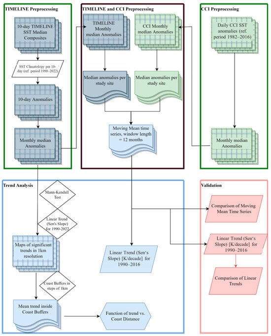
Figure 4.
Flowchart illustrating the workflow of this study. The blue symbols are connected to TIMELINE SST, the green symbols are connected to CCI SST, light-blue symbols are connected to the trend analysis and the salmon-colored symbols are connected to the validation analysis.
3.1. Calculation of Monthly Anomalies
TIMELINE SST anomalies were calculated for the study regions described in Section 2.2. To reduce the seasonal impact, we calculated 10-day anomalies with respect to the period from 1990 to 2022 as defined in Equation (1).
where SSTanomaly (10 days) is the 10-daily anomaly and SSTmedian (10 day) is the median SST in the 10-day period. We then aggregated the 10-day anomalies to monthly mean anomalies to smooth outliers and fill spatial gaps due to cloud cover. For the comparison, the global CCI daily SST anomaly dataset was cropped to the extents of the study areas. To match the temporal resolution of the TIMELINE SST anomalies, the daily CCI anomalies were also aggregated to monthly median anomalies by taking their median for the respective month.
3.2. Calculation of Anomaly Trends per Study Area
The TIMELINE and CCI SST monthly anomalies were aggregated over each of the study areas, taking the median of all available pixels in the respective area. For both of the resulting time series, a moving mean with a window size of one year was applied to display the climatological patterns for each study area and to compare the TIMELINE and CCI time series. Furthermore, the Mann–Kendall test was applied and the Sen’s slope was calculated to analyze and compare significant long-term trends for each study area. Section 4.1 addresses the analysis of TIMELINE SST anomaly time series, whereas Section 4.2 contains the comparison of the CCI and TIMELINE moving mean time series and the long-term trends for each study area.
3.3. Mapping of the Monthly Anomaly Trends
Based on the TIMELINE monthly anomalies described in Section 3.1, the Mann–Kendall test was performed and the Sen’s slope was calculated for each month on a pixel-base. This allowed us to display the significant monthly anomaly trends with one km resolution. The significance level was 5%, meaning that pixels associated with an p-value > 0.05 were masked from the trend maps. The Mann–Kendall trend test as well as the calculation of the Sen’s slope was performed using the “Original Mann–Kendall test” from the pymannkendall package (version 1.4.3) in Python. In Section 4.3, the spatial distribution of the monthly anomaly trends is described.
3.4. Relationship of Linear SST Trend to Coast Distance
Based on the monthly trend maps produced in Section 3.3, we carried out some spatial analysis of the significant trends. The trend in relation to the distance to the coast was analyzed for each study area and for months with a high proportion of significant trends. To that end, we created coast buffers, with an increasing coast distance in steps of 1 km. In between each 1 km step, the mean trend as described in Section 3.1 was calculated and plotted against the coast distance. The calculation was performed in R using the R packages terra and sf. In Section 4.4, we show the results of this analysis.
4. Results
4.1. Analysis of the TIMELINE SST Anomaly Time Series
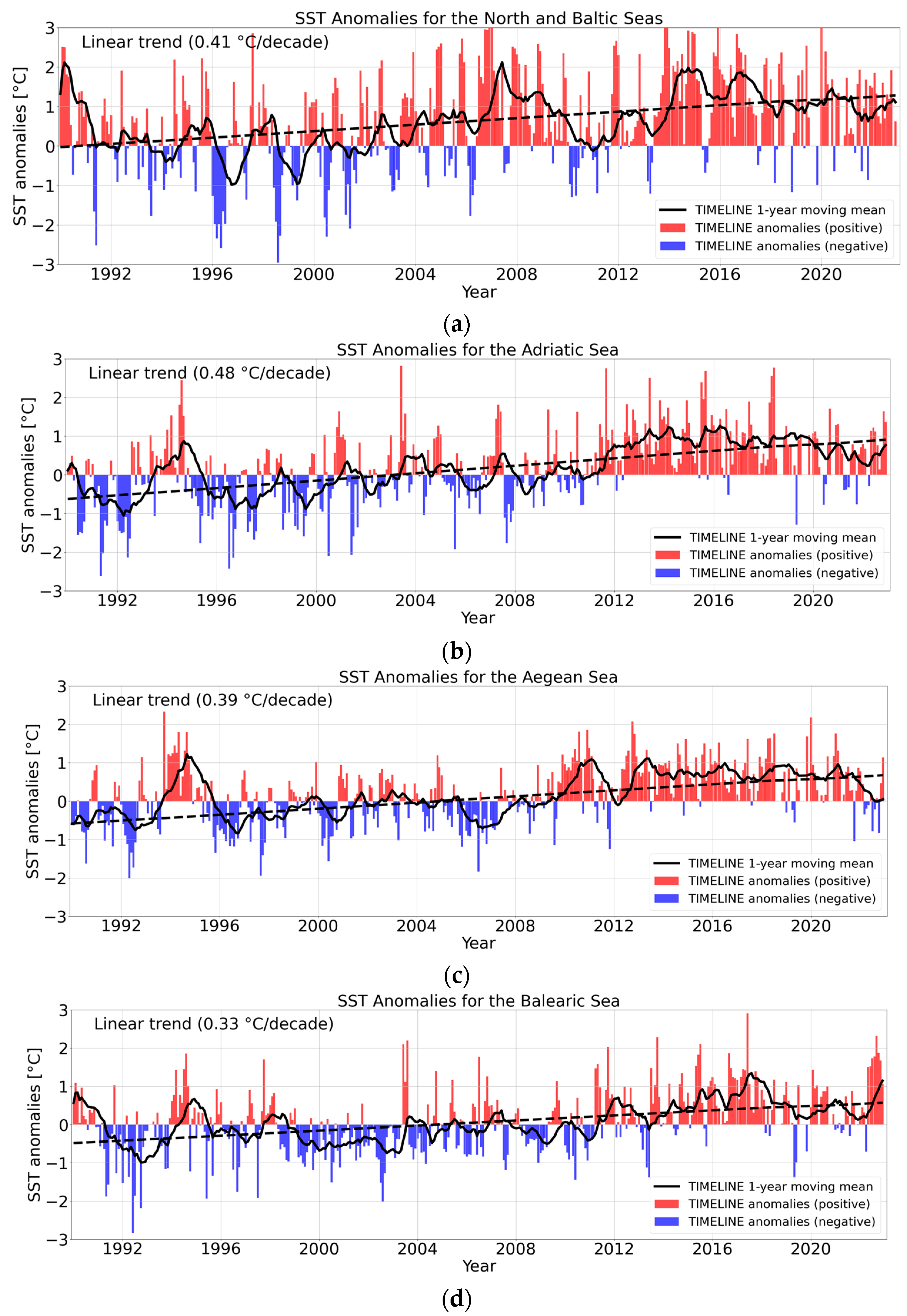
Figure 5 displays the time series of the monthly anomalies, as well as the moving mean and the trend for all study areas. An overview of the study areas and the respective trends is also provided in Table 3. The Adriatic Sea experienced the highest trend with a slope of 0.48 °C/decade, which results in an increase of 1.54 °C for the whole study period. Lower trends have been observed for the other study areas, with 0.41 °C/decade for the North and Baltic Seas, 0.39 °C/decade for the Aegean Sea, and 0.33 °C/decade for the Balearic Sea. For all study areas, the last decade is dominated by high positive anomalies and contributes the most to the SST warming trends.
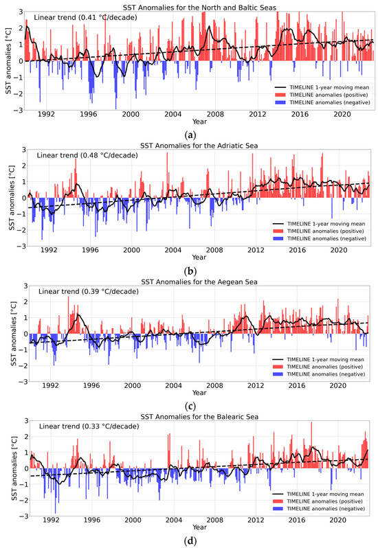
Figure 5.
Monthly SST anomalies and 1-year moving mean for the North and Baltic Seas (a), Adriatic Sea (b), Aegean Sea (c) and Balearic Sea (d).
Table 3.
Linear trend of SST anomaly time series at study sites.
Besides the long-term trends, several warmer and colder periods can be identified, which depend on the respective study area. The cold years of 1993 and 1996 in the North and Baltic Seas fit with [39], who reported that 1996 had the most severe winter in the southern Baltic Sea. For the Adriatic Sea, the cold winter–spring of 1999 is apparent, followed by warmer conditions in the early 2000s [40]. The heatwaves in 2003 and 2006 are visible throughout all study areas, but especially pronounced in the Adriatic Sea in 2003 with anomalies up to 3 °C [41] and the North and Baltic Seas in 2006. The 2006 heatwave was particularly extreme over Scandinavia and Western Europe, and was partly caused by a “blocking” weather regime [42]. It was followed by a colder period between 2008 and 2012, which is again especially visible at the Baltic and North Sea. The ice winter of 2010/11 contrasts the previously mentioned heat waves. In the Baltic Sea, SST decreased very strongly during November and December 2010. The anomalies were the lowest in Kattegat/Skagerrak with −4 K and the western Baltic with −2 to −3 K [39]. From late November to early January, the entire Baltic Sea region was under the influence of cold polar air [43]. After 2015, which was the last cold regime because of a North Atlantic cold anomaly [44], the Baltic sea was marked by several hot months with anomalies regularly higher than 2 K, and only a few single months with negative anomalies.
4.2. Comparison between TIMELINE and CCI SST Anomalies
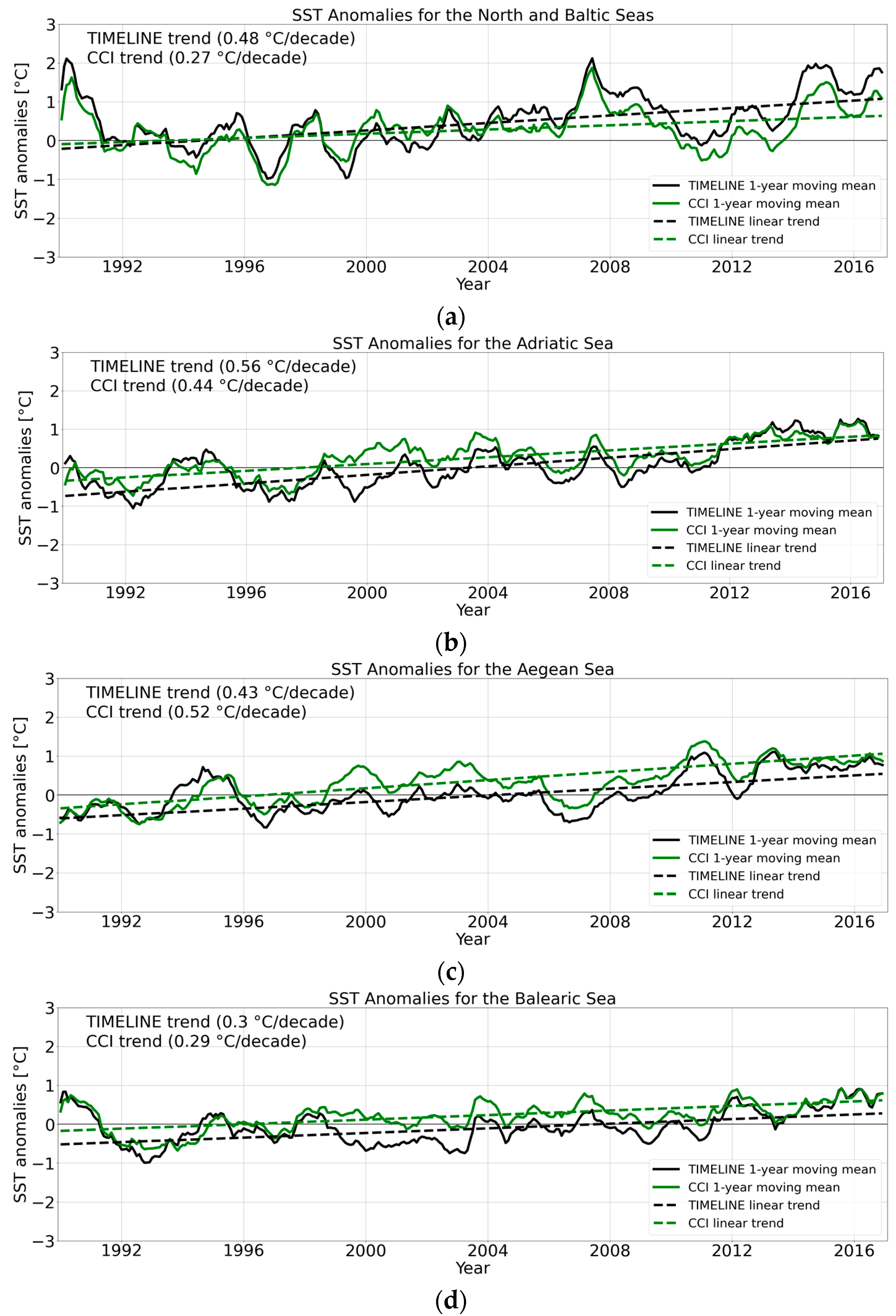
Figure 6 displays a comparison between the TIMELINE and the CCI time series, showing the moving average as well as the long-term trend for each study area for the period 1990–2016. Table 4 presents the result of the correlation between the monthly TIMELINE and CCI anomalies (coefficient R and the root mean square error (RMSE)) as well as the trend differences for the four study areas. It is apparent that the accordance between the TIMELINE and CCI anomalies in the Adriatic Sea, the Aegean Sea, and the Balearic Sea are quite similar with respect to R values, which are between 0.82 and 0.85, and RMSEs between 0.5 and 0.54 °C. Meanwhile, for the North and the Balearic Seas, the accordance is lower with an R value of 0.77 and an RMSE of 0.84 °C. For the Balearic Sea, the TIMELINE trend is similar to the CCI trend, while for the Adriatic and the Aegean Sea, the trend difference is in the order of 20% in relation to the trend. For the North and Baltic Seas, the TIMELINE trend is 75% higher than the CCI trend. Figure 6 reveals that the TIMELINE and CCI moving averages show similar patterns for large parts of the time series for all study areas. Higher differences are visible during the period from 1994 to 1995, where the TIMELINE anomalies are considerably higher than the CCI anomalies in the Mediterranean study areas. Possible causes for that will be discussed in Section 5. Furthermore, there is a positive offset of the CCI towards the TIMELINE moving average for large parts of the time series in all study areas. This offset can be explained by the different reference periods: While the CCI anomalies are based on the period 1982–2016, the TIMELINE anomalies are based on the period 1990–2022. However, because of the higher trends in the TIMELINE anomalies, this offset decreases towards the end of the time series.
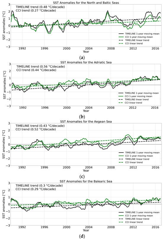
Figure 6.
Comparison of TIMELINE and CCI monthly SST anomalies and the moving mean (window length = 12 months) for the North and Baltic Seas (a), Adriatic Sea (b), Aegean Sea (c) and Balearic Sea (d).
Table 4.
Correlation coefficient R and root mean square error (RMSE) between the TIMELINE and CCI monthly anomalies as well as the trend difference for each study area.
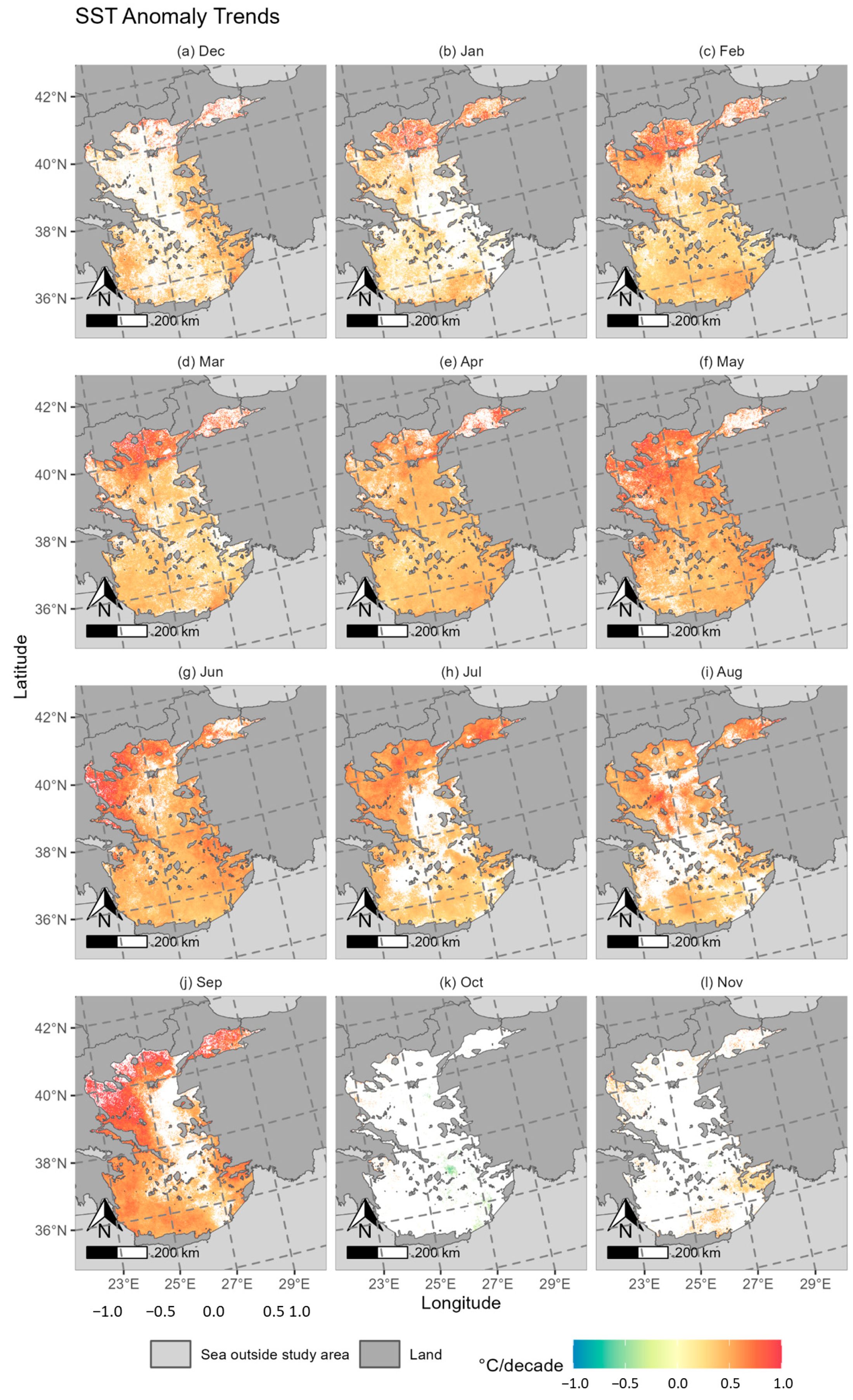
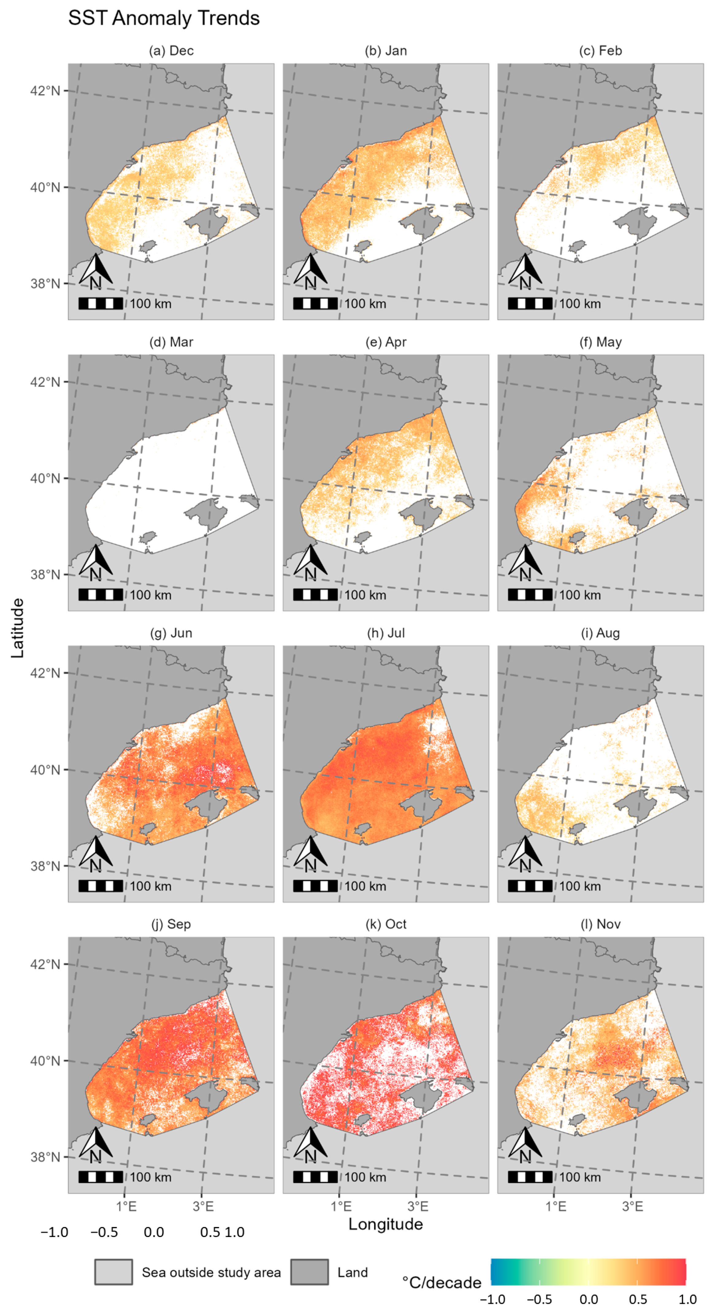
4.3. Spatial Distribution of Anomaly Trends
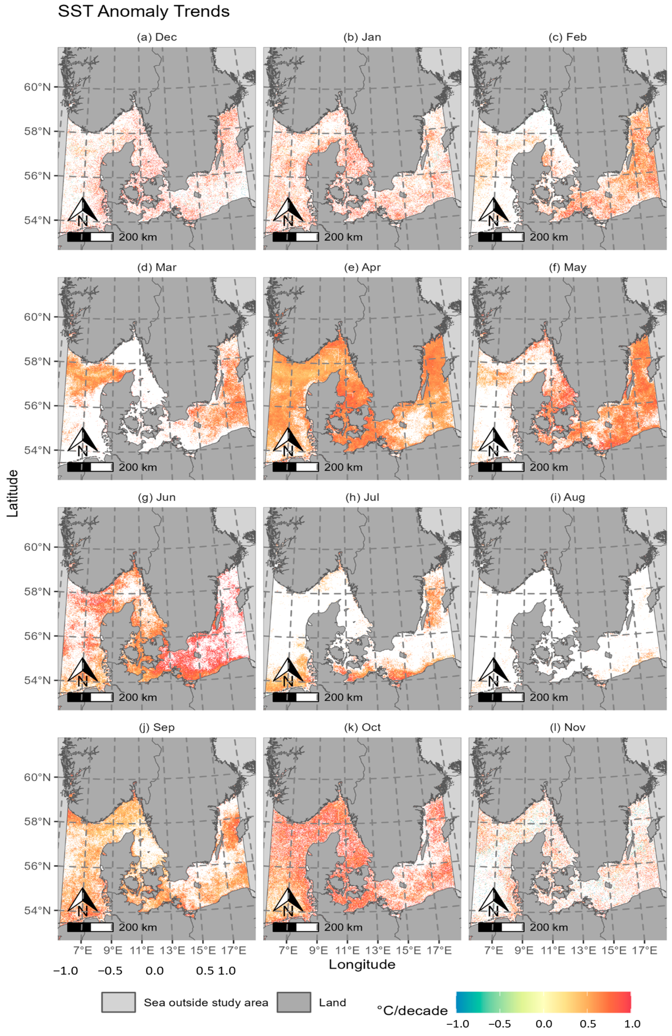
In Figure 7, Figure 8, Figure 9 and Figure 10, we present the spatial distribution of the SST anomaly trends for each month and study area. Overall, we found mostly positive trends. However, the magnitude and spatial distribution of trends showed high variations for both the study areas and the different months. As outlined in Section 3.2, insignificant pixels with p > 0.05 were masked.
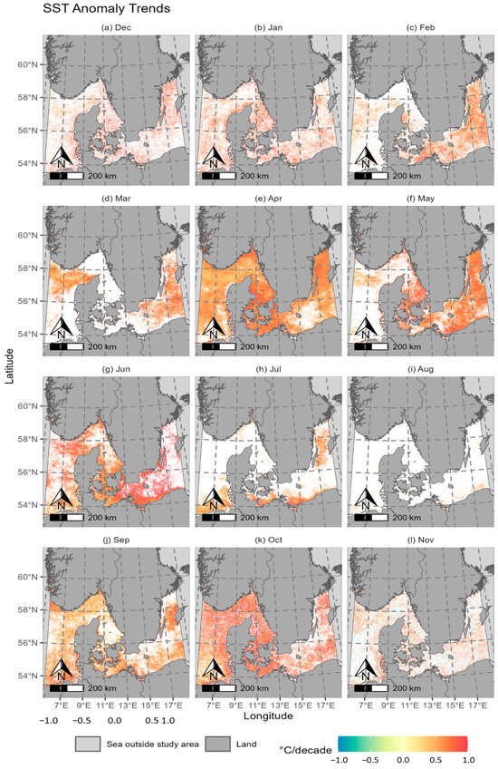
Figure 7.
Spatial distribution of SST trends for each month in the North and Baltic Seas.
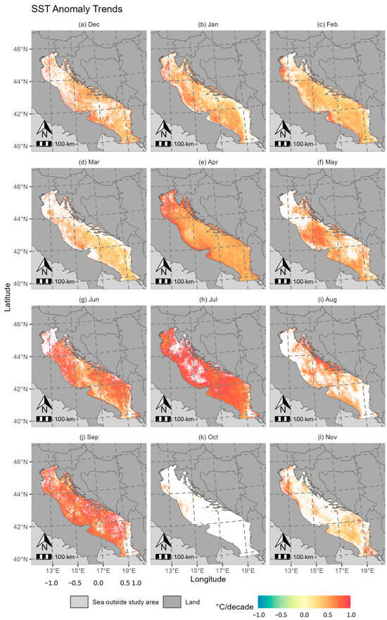
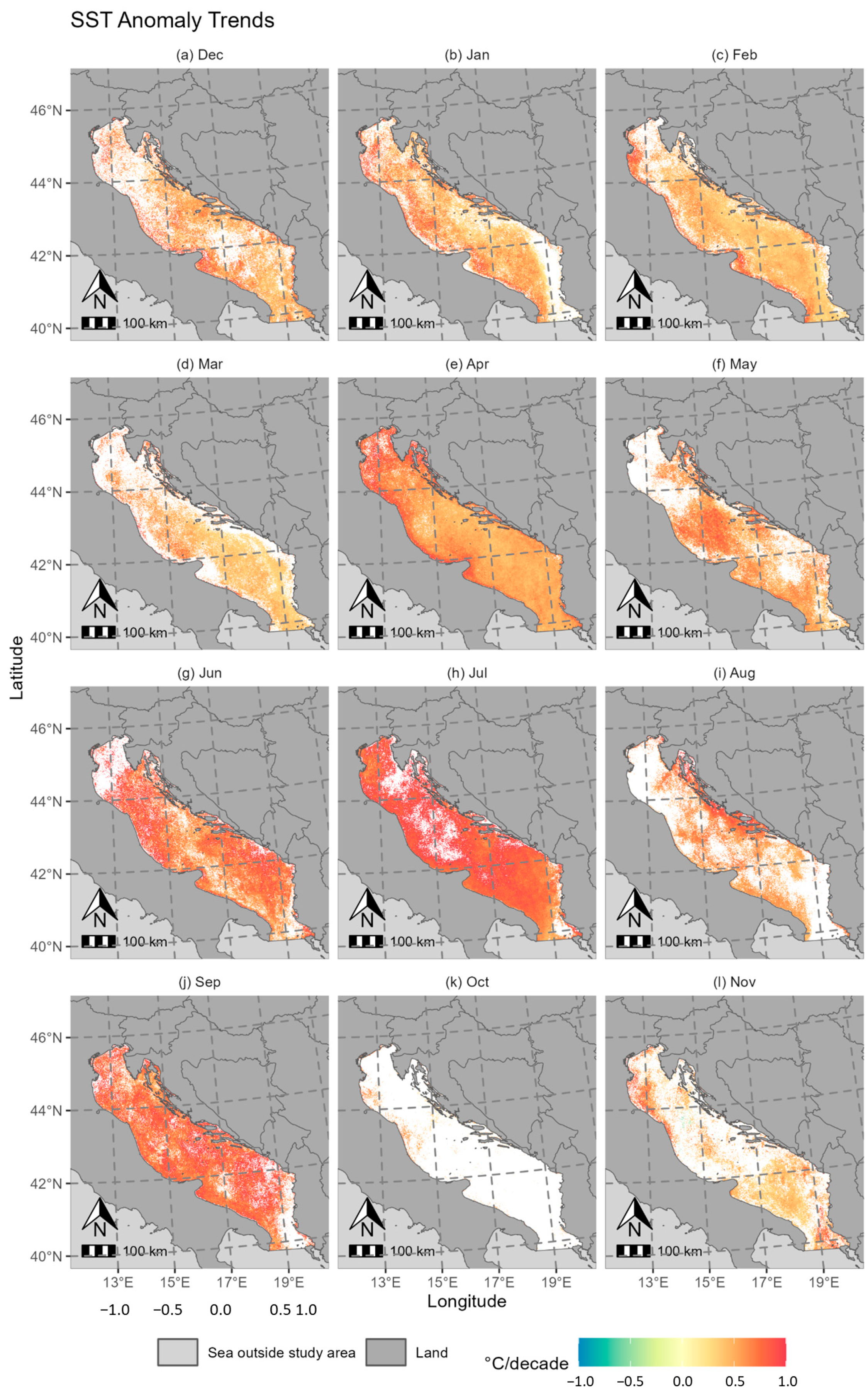
Figure 8.
Spatial distribution of SST trends in the Adriatic Sea for each month.
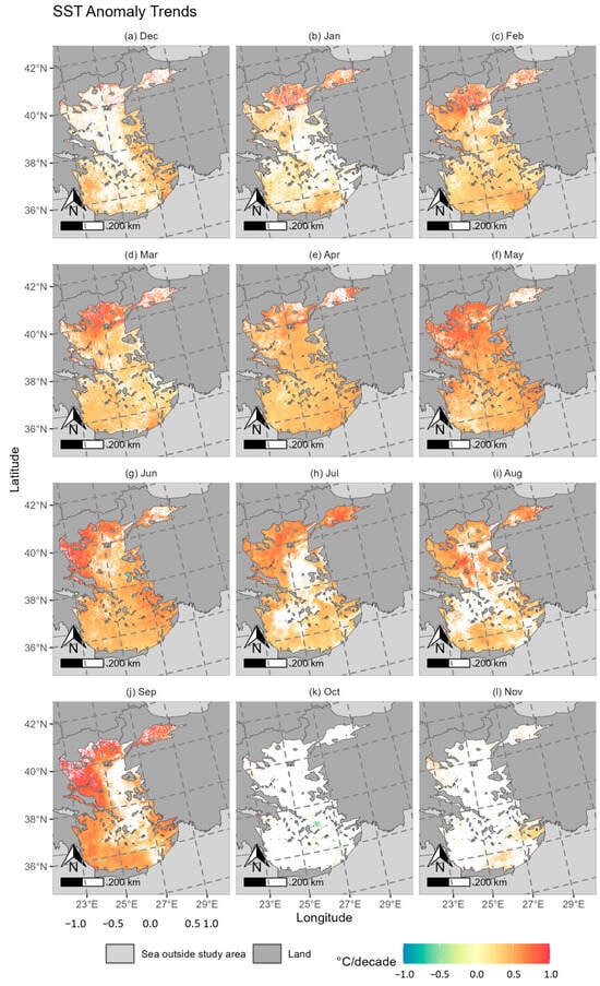
Figure 9.
Spatial distribution of SST trends in the Aegean Sea for each month.

Figure 10.
Spatial distribution of SST trends in the Balearic Sea for each month.
For the North and Baltic Seas (Figure 7), area-wide positive trends are visible throughout March to June as well as for the months September and October. While for March and April high trends are mostly seen along the Danish coast in the Skagerrak and Kattegat (up to 1 °C/decade), between May and July, the highest trends can be observed along the German, Polish, and Swedish Baltic Sea coast. For September, high trends (>0.5 °C/decade) can be observed near Bornholm, while for October, high trends can be observed throughout the whole study area.
For the Adriatic Sea (Figure 8), trends are highest in June, July, and September, exceeding 0.5 °C/decade almost through the whole study area. Especially high trends can be seen along the Italian coast (up to 1 °C/decade) around the Gargano Peninsula and the Gulf of Venice. In the summer months, high trends can also be observed on the Balkan coast.
For the Aegean Sea (Figure 9), high positive trends (>0.5 °C/decade) are visible in the northern part (Thracian Sea and Thermaic Gulf) almost throughout the whole year, with the exception of the period from October to December. The trend is highest in September (up to 1 °C/year). In August, a hotspot with very high trends can be observed north of the island Skyros. The highest trends in the Sea of Marmara can be observed in the summer months from June to September.
For the Balearic Sea (Figure 10), the highest positive trends can be observed in summer and autumn, whereby September and October show very high trends throughout the whole study area. During winter and spring, we can observe moderate to high trends along the Spanish coast (around 0.5 °C/decade), while there are less significant trends in open waters.
4.4. SST Trends in Relation to Coast Distance
Section 4.3 has revealed that nearshore areas show higher SST anomaly trends than open waters. To further investigate this finding, SST trends were analyzed in relation to coast distance for each month. Several months were excluded from this analysis, because they showed significant trends in less than 30% of the respective study area. This was the case for January, February, March, July, August, November, and December in the North and Baltic Seas, October in the Adriatic Sea, October and November in the Aegean Sea, and February, March, May, and August in the Balearic Sea.
Figure 11 shows the SST trend plotted against the distance to the coast for each study area. The trend gradient in relation to distance from the coast is especially visible in spring in the Adriatic Sea; in March, for example, the trend directly at the coast is almost 0.7 °C/decade, while it drops down to 0.4 °C/decade at 40 km distance to the coast. Similarly, in May, the trend at the coast is 0.5 °C/decade and only 0.25 °C/decade at a 40 km distance to the coast. For the other study areas, the trend gradient is not as pronounced as for the Adriatic Sea but still visible. For the Balearic Sea, trends at 10 km from shore are around 0.1 °C/decade lower than trends directly at the coast. For the Aegean Sea, trends drop up to 0.1 °C/decade in the 0–5 km zone to the coast. For the North and Baltic Seas, the picture is more ambiguous: while in April, September, and October, the trend drops within the 0–30 km zone around the coast, for May and June, the trend shows a slight increase with distance to coast. This will be further discussed in Section 5.
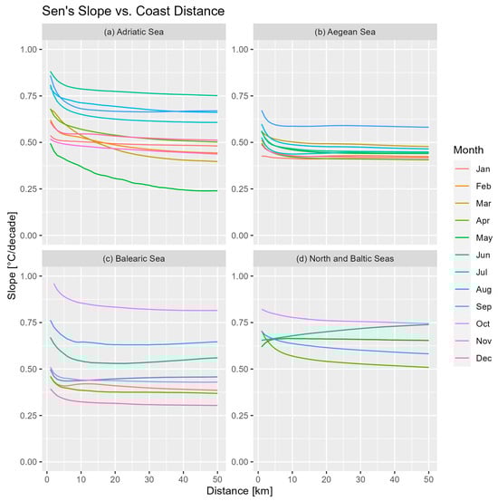
Figure 11.
SST trend (°C/year) per month in relation to coast distance for the study areas.
5. Discussion
5.1. The TIMELINE SST Product and the Generation of the Anomaly Time Series
In this study, we present an analysis of the TIMELINE SST product. The aim was twofold: Firstly, to create new insights into the long-term SST dynamics by considering the recent warm years up to 2022 and applying the enhanced spatial resolution of 1 km in comparison with previous long-term SST studies; secondly, to evaluate the reliability and consistency of the TIMELINE SST time series by comparing it to the established CCI SST time series.
Because of the length of the AVHRR time series, sensors are distributed across several subsequent platforms as new generations have been launched (in the case of this study, NOAA-11, 14, 16, 17, 18, and 19), where each sensor has a different spectral response curve. Furthermore, the NOAA platforms experience orbit drift, which leads to changing observation times throughout the time series [45]. For the TIMELINE SST product, we wanted to make use of the extensive radiative transfer modeling and harmonization of the AVHRR sensors performed by [21] during the development of the TIMELINE Land Surface Temperature product. During the atmospheric and emissivity correction, a different set of parameters was applied for each AVHRR sensor, view angle, water vapor, and temperature level class. For the split window algorithm, we assumed a uniform emissivity for sea surfaces, as was proposed in the original algorithm publication [20]. Given that we only used SST observations acquired with satellite view angles < 50°, depending on wind speed, sea surface emissivity can vary up to 0.01 [46]. Error simulations have shown that this translates into errors up to 0.5 °C for the temperature calculation [21]. However, this would only apply to extreme cases and is not likely to add a systematic error to the SST time series.
In this study, no SST daytime correction was included. Instead, only observations from daytime overpasses were used, which were taken between 8:00 h and 20:00 h. In this time frame, the SST variability is <0.2 °C in the summer and <0.1 °C in the other seasons, which can be derived from diurnal SST cycle models as published by [47]. It was assumed that the SST anomalies due to observation time differences would not significantly impact the SST trend calculation. A further known challenge when dealing with AVHRR data is geolocation errors [14]. Within the TIMELINE project, this problem is tackled with the help of the chip-matching preprocessor, which improves the mean geolocation error of the Level 1b data to 0.92 km [48]. Thus, subpixel accuracy is achieved.
For this study, the trend was calculated on the base of anomalies, which represent the deviation of the long-term climatological mean. Anomalies are a common way in climatology to remove seasonality from the time series. We decided to use 10-day anomalies, as they offer a compromise between low SST variability within 10 days and high data availability within the period. Utilizing the median for this calculation enhances robustness against outliers compared to the mean. Additionally, we aggregated the 10-day anomalies into monthly anomalies to improve the spatial completeness of the results. The combination of the Mann–Kendall significance test and Sen’s slope represents a robust method commonly employed for temperature trend analysis. in contrast to the CCI SST time series, the TIMELINE SST time series is not gap-free, meaning that the data availability within the study areas can differ throughout the time series. Although the possibility exists that this could influence the presented trends, the close alignment between the TIMELINE time series and the CCI time series indicates that our calculated anomalies are a valid representation of the SST dynamics within our study areas. This is further supported by the representation of heat waves and other temperature extremes that have occurred in recent years, which are consistent with the observed dynamics of the TIMELINE SST anomaly time series depicted in our analysis.
5.2. Comparison between TIMELINE and CCI Product
The comparison between the TIMELINE and CCI SST anomaly time series revealed a strong correlation for the Mediterranean study areas (R ≥ 0.82) and lower correlation for the North and Baltic Seas (R = 0.77). Furthermore, the long-term trends were equal for the Balearic Sea, while they were moderately different (~20%) for the Adriatic and the Aegean Sea and significantly different (~75%) for the North and Baltic Seas.
Initially, the differences between the time series can be partially attributed to differences in their respective product generation chains.
The TIMELINE AVHRR SST was derived using the split window algorithm by [20], which was trained with the radiative transfer model MODTRAN. In contrast, the CCI AVHRR SST was calculated using the fast radiative transfer model (RTTOV) [49]. Furthermore, while the TIMELINE AVHRR product assumed uniform emissivity based on [22], the CCI emissivity module considered factors such as wind speed and salinity [13]. Additionally, a daytime correction was applied to the CCI SST product, which was not the case for the TIMELINE SST product. However, as mentioned in the section above, these factors are expected to have only minor influences on the anomaly time series. Finally, the CCI SST anomalies were calculated on the base of the Level 4 SST analysis product, which was spatio-temporally interpolated. This, coupled with the fact that the Level 4 product represents SST at a 20 cm depth, might result in a smoother time series but could also cause a degradation of feature resolution [13].
Besides the differences between the TIMELINE and CCI SST products, there are also differences in the anomaly calculation itself: while the CCI SST anomalies are based on the reference period of 1982–2016, the TIMELINE SST anomalies are calculated based on the reference period of 1990–2022. However, this fact can only lead to a constant offset of the anomalies on the y-axis and do not affect the climatological pattern or trend in the time series. This offset is evident, varying in degree, across all of the plots. Additionally, the monthly TIMELINE SST anomalies were calculated from decadal anomalies, opposed to the CCI anomalies, which were calculated from daily anomalies. Due to the higher variation of SST during a 10-day period compared to a single day, this could lead to a higher standard deviation in the anomalies. Finally, the fact that the CCI SST product is gap-free and has a lower spatial resolution can also lead to different results.
Despite the obvious differences, we argue that comparing our results with the CCI product is relevant. Firstly, the CCI SST product is one of the most used datasets for long-term SST studies [4], and secondly it shows the best agreement with in situ observations [16]. Given the differences in the SST product generation and the SST anomaly calculation described above, the overall high agreement between the CCI and TIMELINE time series makes us confident about our results.
5.3. Discussion and Comparison of SST Trends
Our study found an SST trend for the period of 1990–2022 of 0.48 °C/decade for the Adriatic Sea, 0.41 °C/decade for the North and Baltic Seas, 0.39 °C/decade for the Aegean Sea, and 0.33/decade °C for the Balearic Sea. These trends are much higher than the global SST trend, which is reported to be 0.09 °C/decade for the period of 1982–2018, or 0.11 °C/decade when excluding sea-ice regions [4]. The North, Baltic, and Mediterranean Seas are among the hot spots of SST warming [4,17]. This is also supported by previous studies (see Table 2); e.g., [28] found a warming of SST between 2003 and 2019 of 0.7 °C/decade for the Adriatic Sea, 0.7 °C/decade for the Aegean Sea, and 0.5 °C/decade for the Balearic Sea. For the Baltic Sea, [30] reported an SST warming of 0.41 °C/decade between 1982 and 2012, while [29] reported an SST warming of 0.5 °C/decade between 1982 and 2021. For the North Sea, SST warming of 0.37 °C/decade was reported by [30].
Section 4.3 delineated clear seasonal differences in both the magnitude and spatial distribution of trends. The highest trends in the North and Baltic Seas were observed during spring and early summer (April to June) and early autumn (September to October). Similarly, for the Mediterranean study areas, peak trends occurred during early summer and September. The Adriatic and Aegean Seas showed a similar seasonal pattern with area-wide significant trends from December throughout September and only scattered trends in October and November. The accumulation of high positive trends in spring and early summer suggests a potential seasonal shift, with a progressively earlier warming phase of SST towards the later years. Simultaneously, the high trends in September may indicate a prolongation of the warm SST condition in summer. High SST trends at the Mediterranean coast in spring and autumn were also observed by [17] and interpreted as an indicator for a phenological shift.
While most of the months in Section 4.3 showed area-wide significant trends, some of the months only showed scattered areas or almost no significant trends. For the North and Baltic Seas, this was the case for December, January, July, August, and November; for the Adriatic Sea, this was the case for August, October, November, and December; for the Aegean Sea, this was the case for December, October, and November; and for the Balearic Sea, this was the case for December, February, March, and May. For the analysis of the significant trends, we decided to mask trends with a p-value higher than 0.05, which is common for SST analysis but also represents a high significance level. Figures S5–S8 in the Supplementary Materials show maps of the p-value for each month and study area. For the winter months, we see p-values higher than 0.4, which clearly indicate no significant trend. These low p-values can be explained by higher cloud cover in the winter months, which leads to fewer observations. However, for July in the North and Baltic Seas, August in the Adriatic Sea, and May in the Balearic Sea, we see large areas with p-values around 0.1, which could indicate a weak significant trend.
5.4. Importance of the Monitoring of SST Trends in Coastal Areas
Significantly higher SST warming rates in coastal areas were already reported in prior studies, e.g., by [17]. In Section 4.4, we observed a clear SST trend gradient relative to the distance from the coast. This gradient was particularly distinct in the Adriatic Sea during spring. Here, the trend at the coast in March and May was twice as high as that observed at a 40 km distance to coast. The width of the near-coastal zone, where this gradient was visible, varied between the study areas: for the Adriatic Sea it was 40 km, for the Balearic Sea it was 10 km, and for the Aegean Sea it was only 5 km.
Coastal areas represent some of the most biodiverse and also variable environments of the ocean [50]. But these areas are also exposed to extraordinary anthropogenic pressure such as overpopulation, agricultural runoff and pollution, overfishing, and maritime traffic [51]. High SST warming rates can be an additional threat to these vulnerable ecosystems and can have an impact on key biological processes. One example is the phenology and productivity of phytoplankton, which shows a clear response to SST warming [5]. Besides ecological consequences, high SST warming rates can also have a major economic impact: the aforementioned changes in plankton had a proven negative influence on the biomass and landings of European anchovy and sardine, which are among the most popular seafood [6]. Furthermore, changes in SST affect the aquaculture industry [7]. Indirect consequences of SST trends on tourism are also possible, as seen for example in the algae blooms of the recent years in the Baltic Sea, which are favored by high SSTs [8].
Our analysis regarding the SST trends in relation to coast distance has shown that the SST trends in coastal areas can vary significantly on a kilometer scale. Differently from open sea conditions, where SST trends are mostly determined by large-scale ocean circulations and atmospheric warming, near-coast SST trends are also influenced by topography or local atmospheric and oceanographic circulation patterns [19]. While for the Mediterranean study areas the near-coast trends were consistently higher in comparison to open waters, the trend gradient in the North and Baltic Seas for June was the other way around. This pattern could point to upwelling events, which can cause a depression of warming rates [19]. Our increased resolution of 1 km can contribute to a deeper understanding of the impact of local factors on SST warming and thus help policymakers to make more sustainable decisions.
5.5. Outlook and Further Development of the TIMELINE SST Product
This study has demonstrated the potential of AVHRR LAC data with 1 km spatial resolution to reliably map long-term trends of SST in areas with high spatial SST variability, particularly coastal areas. While the TIMELINE SST product has not reached the maturity of well-established long-term SST products, such as for example the CCI SST product [13] or the AVHRR pathfinder product [12], our analysis revealed generally good agreement with the findings of previous studies. Further developments are planned to improve the accuracy and stability of the TIMELINE SST dataset. Hereby, many findings from the generation of the CCI SST dataset can be possibly adapted: as previously mentioned, the split window algorithm used for TIMELINE SST calculation [20,21] does not yet consider the impact of wind speed and salinity on the sea surface emissivity. An appropriate emissivity module could improve the accuracy of the product [52]. Moreover, daytime correction should be integrated into the processing chain. This not only prevents artefacts in the time series due to orbital drift but also allows the integration of morning, evening, and nighttime observations thus enhancing the data availability. Areawide daytime correction for SST can either be derived from the time series itself by setting noon observations as a reference [13] or from observations by geostationary satellites [53]. While sea ice did not impact our study areas, sea ice detection will soon be integrated into the TIMELINE processing chain to enable the analysis of the time series even at high latitudes.
In this study, spatial completeness throughout the time series was nearly accomplished by using 10-day composites of SST. While the median proved to be suitable in terms of representativeness, daily anomalies could offer a more accurate picture of time series patterns and trends. Gap-free daily datasets were calculated by the CCI group by using an assimilation approach; however, this comes with the price of losing spatial feature resolution [13]. For the TIMELINE SST dataset, we are exploring solutions to create a reliable daily gap-free dataset while retaining high spatial resolution. The resulting products would allow for follow-up analysis and relating SST trends spatially to other related variables like bathymetry or wind speed. Finally, validation of the TIMELINE SST towards buoy measurements and other satellite-derived SST products should be extended in terms of accuracy, precision, and stability.
6. Conclusions
SST is a key indicator of climate change. It plays a pivotal role in global lateral energy transport, radiative air–sea energy exchange, absorption of anthropogenic greenhouse gases in the ocean, modification of the atmospheric boundary layer, and the global water cycle. Furthermore, changes in SST have significant impacts on marine ecosystems, and therefore need to be closely monitored. Satellite-derived SST has been extensively studied. However, coastal regions have received less attention, although they experience significant SST increases and represent some of the most biodiverse and variable environments of the ocean. Elevated SST poses threats to biodiversity and fundamental biological processes and also has economic consequences including negative effects on fisheries, aquaculture, and potential impacts on tourism. To understand SST trends in coastal areas, long-term SST datasets with high spatial and temporal resolution are necessary, which can be provided by AVHRR LAC data with 1 km resolution.
This research introduces the TIMELINE SST product, a unique dataset providing over 30 years of SST observations at a 1 km resolution. The study focuses on four significant European regions—the Northern and Baltic Seas, the Adriatic Sea, the Aegean Sea, and the Balearic Sea—chosen for their extensive nearshore areas and economic/ecological importance. For these areas, we analyzed monthly SST anomaly trends between 1990 and 2022 and mapped their spatial distribution with a 1 km resolution. We compared the trends to prior SST studies and to anomaly trends derived from the CCI SST product. Furthermore, we mapped the significant trends with a 1 km resolution for each study area and each month and analyzed the spatial distribution with regards to coast distance.
We found mostly positive trends for all study areas. Regarding the whole areas, we found a trend of 0.41 °C/decade for the North and Baltic Seas, 0.48 °C/decade for the Adriatic Sea, 0.39 °C/decade for the Aegean Sea, and 0.33 °C/decade for the Balearic Sea. These trends exceed the global SST trend of 0.11 °C/decade and highlight these regions as hotspots of SST warming. Seasonal variations were noted, with the highest trends observed during spring, early summer, and early autumn. This pattern could indicate a prolongation of the warm SST phase in summer and thus a seasonal shift. Regarding the spatial distribution, an SST trend gradient was observed with higher trends near the coast and lower trends in open waters. The gradient was especially distinct in the Adriatic Sea during spring, where the trend at the coast in March and May was twice as high as that at a 40 km distance to coast. The differences between near-coast and open water trends can be attributed to topography, local atmospheric conditions, and oceanographic circulation patterns. The increased resolution of 1 km of the TIMELINE SST dataset can help to obtain a more accurate picture of these small-scale variations of SST trends.
The observed long-term trends in the study areas are in line with previous SST studies. The comparison between the TIMELINE and CCI SST time series showed high correlations of the anomalies in the Mediterranean study areas but lower correlation in the North and Baltic Seas. Long-term trends differ significantly in the North and Baltic Seas, moderately in the Adriatic and Aegean Seas, and are similar in the Balearic Sea. Differences in the product generation chains, including algorithms, emissivity assumptions, and daytime correction can explain these variations in the time series. Furthermore, the anomalies were calculated with different reference periods, and the temporal resolution differs. Despite these discrepancies, the comparison is considered relevant, as the CCI product is widely used in long-term SST studies and aligns well with in situ observations.
This study highlights the potential of AVHRR LAC data with 1 km spatial resolution for mapping long-term SST trends in areas with high spatial SST variability, such as coastal regions. Further improvements of the TIMELINE SST product are planned, which comprise an enhanced emissivity module to account for wind speed and salinity impacts, daytime correction to prevent artifacts from AVHRR orbital drift and enhance data availability, and sea ice detection. Furthermore, we are exploring methods for creating a daily gap-free dataset which preserves the high spatial resolution of the AVHRR LAC data. In the meantime, we are extending the validation of the product. Further in-depth analyses are planned, which can help to understand the dynamics of SST warming in coastal regions.
Supplementary Materials
The following supporting information can be downloaded at: https://www.mdpi.com/article/10.3390/rs16111932/s1, Figure S1: TIMELINE SST against in situ SST measured at NOAA drifting buoys between 2007 and 2013 for 195 buoys; Figure S2: Difference between TIMELINE and CCI monthly maximum SST for the North Sea (a) and the Baltic Sea (b). The dark blue line shows the median difference, while the shaded areas show the 5–95% quantiles of the difference; Figure S3: Difference between TIMELINE and CCI SST for three 10-daily maximum composites in summer (a–c) and in winter (d–f) classified for classes of Total Columnar Water Vapor (TCWV [kg/m2]) and satellite view angle (VA [°]); Figure S4: Difference between the 1-year rolling means of the TIMELINE and CCI SST anomalies for the North and Baltic Sea as displayed in Figure 6a); Figure S5: p-values in the North and Baltic Seas; Figure S6: p-values in the Adriatic Sea; Figure S7: p-values in the Aegean Sea; Figure S8: p-values in the North and Balearic Sea.
Author Contributions
Conceptualization: P.R.; data curation: P.R.; investigation, formal analysis, and visualization: L.O. and P.R.; methodology and software: P.R. and L.O.; project administration: S.H.; supervision: C.K.; writing—original draft: P.R. and L.O.; writing—review and editing: S.H., C.K. and A.D. All authors have read and agreed to the published version of the manuscript.
Funding
This research was funded by the German Aerospace Center (DLR) TIMELINE project. This research is associated to the BMBF Metascales project (funding no.: 03F0955G).
Data Availability Statement
The data presented in this study are available on request from the corresponding author. The data are not publicly available due to ongoing research.
Acknowledgments
The authors thank the entire TIMELINE team for fruitful cooperation and discussion. We thank the DLR headquarters for the funding of the TIMELINE project. We thank Kjirsten Coleman for final proofreading.
Conflicts of Interest
The authors declare no conflicts of interest.
References
- Global Climate Observing System. GCOS WMO Essential Climate Variables. Available online: https://gcos.wmo.int/en/essential-climate-variables/sst (accessed on 24 January 2024).
- OOPC. EOV Spec Sheet: Sea Surface Temperature; OOPC: Paris, France, 2017. [Google Scholar]
- O’Carroll, A.G.; Armstrong, E.M.; Beggs, H.; Bouali, M.; Casey, K.S.; Corlett, G.K.; Dash, P.; Donlon, C.; Gentemann, C.L.; Høyer, J.L.; et al. Observational needs of sea surface temperature. Front. Mar. Sci. 2019, 6, 420. [Google Scholar] [CrossRef]
- Bulgin, C.E.; Merchant, C.J.; Ferreira, D. Tendencies, variability and persistence of sea surface temperature anomalies. Sci. Rep. 2020, 10, 7986. [Google Scholar] [CrossRef] [PubMed]
- Hoegh-Guldberg, O.; Bruno, J.F. The Impact of Climate Change on the World’s Marine Ecosystems. Science 2010, 328, 1523–1528. [Google Scholar] [CrossRef] [PubMed]
- Coll, M.; Albo-Puigserver, M.; Navarro, J.; Palomera, I.; Dambacher, J. Who is to blame? Plausible pressures on small pelagic fish population changes in the Northwestern Mediterranean Sea. Mar. Ecol. Prog. Ser. 2018, in press. [Google Scholar] [CrossRef]
- Hartog, J.R.; Spillman, C.M.; Smith, G.; Hobday, A.J. Forecasts of marine heatwaves for marine industries: Reducing risk, building resilience and enhancing management responses. Deep Sea Res. Part II Top. Stud. Oceanogr. 2023, 209, 105276. [Google Scholar] [CrossRef]
- Munkes, B.; Löptien, U.; Dietze, H. Cyanobacteria blooms in the Baltic Sea: A review of models and facts. Biogeosciences 2021, 18, 2347–2378. [Google Scholar] [CrossRef]
- The Copernicus Programme. Record-Breaking North Atlantic Ocean Temperatures Contribute to Extreme Marine Heatwaves. Available online: https://climate.copernicus.eu/record-breaking-north-atlantic-ocean-temperatures-contribute-extreme-marine-heatwaves (accessed on 7 December 2023).
- National Oceanic and Atmospheric Administration. Annual 2022 Global Climate Report. Available online: https://www.ncei.noaa.gov/access/monitoring/monthly-report/global/202213 (accessed on 7 December 2023).
- NASA/JPL. MODIS Aqua Level 3 SST Thermal IR Monthly 4 km Daytime V2019.0; NASA/JPL/PODAAC: Pasadena, CA, USA, 2020. [Google Scholar] [CrossRef]
- Baker-Yeboah, S.; Saha, K.; Zhang, D.; Casey, K.S.; Evans, R.; Kilpatrick, K.A. AVHRR Pathfinder Version 5.3 Level 3 Collated (L3C) Global 4km Sea Surface Temperature for 1981-Present; NOAA National Centers for Environmental Information: Asheville, NC, USA, 2018. [Google Scholar]
- Merchant, C.J.; Embury, O.; Bulgin, C.E.; Block, T.; Corlett, G.K.; Fiedler, E.; Good, S.A.; Mittaz, J.; Rayner, N.A.; Berry, D.; et al. Satellite-based time-series of sea-surface temperature since 1981 for climate applications. Sci. Data 2019, 6, 223. [Google Scholar] [CrossRef] [PubMed]
- Dech, S.; Holzwarth, S.; Asam, S.; Andresen, T.; Bachmann, M.; Boettcher, M.; Dietz, A.; Eisfelder, C.; Frey, C.; Gesell, G.; et al. Potential and challenges of harmonizing 40 years of avhrr data: The timeline experience. Remote Sens. 2021, 13, 3618. [Google Scholar] [CrossRef]
- Eisfelder, C.; Asam, S.; Hirner, A.; Reiners, P.; Holzwarth, S.; Bachmann, M.; Gessner, U.; Dietz, A.; Huth, J.; Bachofer, F.; et al. Seasonal Vegetation Trends for Europe over 30 Years from a Novel Normalised Difference Vegetation Index (NDVI) Time-Series—The TIMELINE NDVI Product. Remote Sens. 2023, 15, 3616. [Google Scholar] [CrossRef]
- Biguino, B.; Antunes, C.; Lamas, L.; Jenkins, L.J.; Dias, J.M.; Haigh, I.D.; Brito, A.C. 40 years of changes in sea surface temperature along the Western Iberian Coast. Sci. Total Environ. 2023, 888, 164193. [Google Scholar] [CrossRef]
- Lima, F.P.; Wethey, D.S. Three decades of high-resolution coastal sea surface temperatures reveal more than warming. Nat. Commun. 2012, 3, 704. [Google Scholar] [CrossRef] [PubMed]
- Santos, F.; Gomez Gesteira, M.; DeCastro, M. Coastal and oceanic SST variability along the western Iberian Peninsula. Cont. Shelf Res. 2011, 31, 2012–2017. [Google Scholar] [CrossRef]
- Varela, R.; Lima, F.P.; Seabra, R.; Meneghesso, C.; Gómez-Gesteira, M. Coastal warming and wind-driven upwelling: A global analysis. Sci. Total Environ. 2018, 639, 1501–1511. [Google Scholar] [CrossRef] [PubMed]
- Becker, F.; Li, Z.-L.; Becker, F.; Li, Z. Towards a local split window method over land surfaces. Remote Sens. 1990, 11, 369–393. [Google Scholar] [CrossRef]
- Frey, C.M.; Kuenzer, C.; Dech, S. Assessment of mono- and split-window approaches for time series processing of LST from AVHRR—A TIMELINE round robin. Remote Sens. 2017, 9, 72. [Google Scholar] [CrossRef]
- Caselles, E.; Valor, E.; Abad, F.; Caselles, V. Automatic classification-based generation of thermal infrared land surface emissivity maps using AATSR data over Europe. Remote Sens. Environ. 2012, 124, 321–333. [Google Scholar] [CrossRef]
- Klüser, L.; Killius, N.; Gesell, G. APOLLO_NG—A probabilistic interpretation of the APOLLO legacy for AVHRR heritage channels. Atmos. Meas. Tech. Discuss. 2015, 8, 4413–4449. [Google Scholar] [CrossRef]
- Ships4SST. Recommended ISFRN L2R Data Specification and User Manual v1.2 rev0.doc; The International Sea Surface Temperature (SST) Fiducial Reference Measurement (FRM) Radiometer Network (ISFRN): Southampton, UK, 2019. [Google Scholar]
- Elipot, S.; Sykulski, A.; Lumpkin, R.; Centurioni, L.; Pazos, M. A dataset of hourly sea surface temperature from drifting buoys. Sci. Data 2022, 9, 567. [Google Scholar] [CrossRef]
- Reiners, P.; Holzwarth, S.; Asam, S. LONGTERM DYNAMICS OF SEA SURFACE TEMPERATURE IN EUROPE BETWEEN 1982 AND 2018: EXPLORING THE NEW TIMELINE AVHRR SST PRODUCT. In Proceedings of the International Geoscience and Remote Sensing Symposium (IGARSS) 2022, Kuala Lumpur, Malaysia, 17–22 July 2022. [Google Scholar]
- Good, S.A.; Embury, O.; Bulgin, C.E.; Mittaz, J. Level 4 Analysis Climate Data Record; Centre for Environmental Data Analysis: Chilton, UK, 2019. [Google Scholar] [CrossRef]
- García-Monteiro, S.; Sobrino, J.A.; Julien, Y.; Sòria, G.; Skokovic, D. Surface Temperature trends in the Mediterranean Sea from MODIS data during years 2003–2019. Reg. Stud. Mar. Sci. 2022, 49, 102086. [Google Scholar] [CrossRef]
- Jamali, S.; Ghorbanian, A.; Abdi, A.M. Satellite-Observed Spatial and Temporal Sea Surface Temperature Trends of the Baltic Sea between 1982 and 2021. Remote Sens. 2023, 15, 102. [Google Scholar] [CrossRef]
- Høyer, J.L.; Karagali, I. Sea surface temperature climate data record for the North Sea and Baltic Sea. J. Clim. 2016, 29, 2529–2541. [Google Scholar] [CrossRef]
- Dutheil, C.; Meier, H.E.M.; Gröger, M.; Börgel, F. Understanding past and future sea surface temperature trends in the Baltic Sea. Clim. Dyn. 2022, 58, 3021–3039. [Google Scholar] [CrossRef]
- Belkin, I.M. Rapid warming of Large Marine Ecosystems. Prog. Oceanogr. 2009, 81, 207–213. [Google Scholar] [CrossRef]
- Meier, M.; Eilola, K.; Almroth-Rosell, E.; Schimanke, S.; Kniebusch, M.; Höglund, A.; Pemberton, P.; Liu, Y.; Väli, G.; Saraiva, S. Disentangling the impact of nutrient load and climate changes on Baltic Sea hypoxia and eutrophication since 1850. Clim. Dyn. 2019, 53, 1145–1166. [Google Scholar] [CrossRef]
- Jeffries, M.A.; Lee, C.M. A climatology of the northern Adriatic Sea’s response to bora and river forcing. J. Geophys. Res. Ocean. 2007, 112, C03S02. [Google Scholar] [CrossRef]
- Bonacci, O.; Vrsalović, A. Differences in Air and Sea Surface Temperatures in the Northern and Southern Part of the Adriatic Sea. Atmosphere 2022, 13, 1158. [Google Scholar] [CrossRef]
- Grbec, B.; Matić, F.; Beg Paklar, G.; Morović, M.; Popović, R.; Vilibić, I. Long-Term Trends, Variability and Extremes of In Situ Sea Surface Temperature Measured Along the Eastern Adriatic Coast and its Relationship to Hemispheric Processes. Pure Appl. Geophys. 2018, 175, 4031–4046. [Google Scholar] [CrossRef]
- Shaltout, M.; Omstedt, A. Recent sea surface temperature trends and future scenarios for the Mediterranean Sea. Oceanologia 2014, 56, 411–443. [Google Scholar] [CrossRef]
- La Violette, P.E.; Tintoré, J.; Font, J. The surface circulation of the Balearic Sea. J. Geophys. Res. Ocean. 1990, 95, 1559–1568. [Google Scholar] [CrossRef]
- Siegel, H.; Gerth, M.; Tschersich, G. Sea surface temperature development of the Baltic Sea in the period 1990–2004. Oceanologia 2006, 48, 119–131. [Google Scholar]
- Böhm, E.; Banzon, V.; D’Acunzo, E.; D’Ortenzio, F.; Santoleri, R. Adriatic Sea surface temperature and ocean colour variability during the MFSPP. Ann. Geophys. 2003, 21, 137–149. [Google Scholar] [CrossRef]
- Feudale, L.; Shukla, J. Influence of sea surface temperature on the European heat wave of 2003 summer. Part I: An observational study. Clim. Dyn. 2011, 36, 1691–1703. [Google Scholar] [CrossRef]
- Chiriaco, M.; Bastin, S.; Yiou, P.; Haeffelin, M.; Dupont, J.C.; Stéfanon, M. European heatwave in July 2006: Observations and modeling showing how local processes amplify conducive large-scale conditions. Geophys. Res. Lett. 2014, 41, 5644–5652. [Google Scholar] [CrossRef]
- Schmelzer, N.; Holfort, J. The ice winter of 2010/11 on the German North and Baltic Sea coasts and a brief description of ice conditions in the entire Baltic Sea region Baltic Sea. 2013, p. 18. Available online: https://www.bsh.de/EN/DATA/Predictions/Ice_reports_and_ice_charts/_Anlagen/Downloads/Description-ice-winters/Description-of-the-ice-winters-2010-2011.pdf?__blob=publicationFile&v=2 (accessed on 20 May 2024).
- Sanders, R.N.C.; Jones, D.C.; Josey, S.A.; Sinha, B.; Forget, G. Causes of the 2015 North Atlantic cold anomaly in a global state estimate. Ocean Sci. 2022, 18, 953–978. [Google Scholar] [CrossRef]
- Julien, Y.; Sobrino, J.A. Correcting AVHRR Long Term Data Record V3 estimated LST from orbital drift effects. Remote Sens. Environ. 2012, 123, 207–219. [Google Scholar] [CrossRef]
- Masuda, K.; Takashima, T.; Takayama, Y. Emissivity of pure and sea waters for the model sea surface in the infrared window regions. Remote Sens. Environ. 1988, 24, 313–329. [Google Scholar] [CrossRef]
- Morak-Bozzo, S.; Merchant, C.; Kent, E.; Berry, D.; Carella, G. Climatological diurnal variability in sea surface temperature characterized from drifting buoy data. Geosci. Data J. 2016, 3, 20–28. [Google Scholar] [CrossRef]
- Dietz, A.J.; Frey, C.M.; Ruppert, T.; Bachmann, M.; Kuenzer, C.; Dech, S. Automated Improvement of Geolocation Accuracy in AVHRR Data Using a Two-Step Chip Matching Approach—A Part of the TIMELINE Preprocessor. Remote Sens. 2017, 9, 303. [Google Scholar] [CrossRef]
- Saunders, R.; Hocking, J.; Turner, E.; Rayer, P.; Rundle, D.; Brunel, P.; Vidot, J.; Roquet, P.; Matricardi, M.; Geer, A.; et al. An update on the RTTOV fast radiative transfer model (currently at version 12). Geosci. Model Dev. 2018, 11, 2717–2737. [Google Scholar] [CrossRef]
- Gray, J.S. Marine biodiversity: Patterns, threats and conservation needs. Biodivers. Conserv. 2004, 6, 153–175. [Google Scholar] [CrossRef]
- Halpern, B.; Walbridge, S.; Selkoe, K.; Kappel, C.; Micheli, F.; D’Agrosa, C.; Bruno, J.; Casey, K.; Ebert, C.; Fox, H.; et al. A Global Map of Human Impact on Marine Ecosystems. Science 2008, 319, 948–952. [Google Scholar] [CrossRef] [PubMed]
- Embury, O.; Merchant, C.; Filipiaú, M. Refractive Indices (500–3500 cm−1) and Emissivity (600–3350 cm−1) of Pure Water and Seawater; Edinburgh Data Share: Edinburgh, UK, 2008. [Google Scholar] [CrossRef]
- Karagali, I.; Høyer, J. Characterisation and quantification of regional diurnal SST cycles from SEVIRI. Ocean Sci. 2014, 10, 745–758. [Google Scholar] [CrossRef]


Disclaimer/Publisher’s Note: The statements, opinions and data contained in all publications are solely those of the individual author(s) and contributor(s) and not of MDPI and/or the editor(s). MDPI and/or the editor(s) disclaim responsibility for any injury to people or property resulting from any ideas, methods, instructions or products referred to in the content. |
© 2024 by the authors. Licensee MDPI, Basel, Switzerland. This article is an open access article distributed under the terms and conditions of the Creative Commons Attribution (CC BY) license (https://creativecommons.org/licenses/by/4.0/).