Towards Urban Digital Twins: A Workflow for Procedural Visualization Using Geospatial Data

Abstract

A key feature for urban digital twins (DTs) is an automatically generated detailed 3D representation of the built and unbuilt environment from aerial imagery, footprints, LiDAR, or a fusion of these. Such 3D models have applications in architecture, civil engineering, urban planning, construction, real estate, Geographical Information Systems (GIS), and many other areas. While the visualization of large-scale data in conjunction with the generated 3D models is often a recurring and resource-intensive task, an automated workflow is complex, requiring many steps to achieve a high-quality visualization. Methods for building reconstruction approaches have come a long way, from previously manual approaches to semi-automatic or automatic approaches. This paper aims to complement existing methods of 3D building generation. First, we present a literature review covering different options for procedural context generation and visualization methods, focusing on workflows and data pipelines. Next, we present a semi-automated workflow that extends the building reconstruction pipeline to include procedural context generation using Python and Unreal Engine. Finally, we propose a workflow for integrating various types of large-scale urban analysis data for visualization. We conclude with a series of challenges faced in achieving such pipelines and the limitations of the current approach. However, the steps for a complete, end-to-end solution involve further developing robust systems for building detection, rooftop recognition, and geometry generation and importing and visualizing data in the same 3D environment, highlighting a need for further research and development in this field.

1. Introduction

The urban environment is a complex and dynamic system that is subject to continuous evolution and change [1]. In the field of urban planning and urban analysis, traditional methods have often struggled to keep pace with these rapid changes. The use of remote sensing data has become more accessible over the past decade, providing more accessible means for regular monitoring and collection of urban data [2]. In this context, DTs [2], virtual replicas of the physical world, have become a popular approach for simulating and analyzing the urban environment.

Traditional 3D modeling approaches for creating DTs, while useful, are often time-consuming and inflexible [3,4]. In contrast, procedural model generation provides a more flexible workflow. It enables the automatic regeneration of the virtual built environment as new data become available, addressing one of the key limitations of conventional methods [5,6].

In recent years, the concept of urban DTs has emerged in the context of urban modeling and planning [1]. DTs can represent a city through its physical assets [7] by creating a digital replica of the physical asset and its rich semantic data that represent city processes [2]. They can potentially address the challenges of effective decision making in complex systems like cities [8].

The Digital Twin Cities Center at Chalmers (DTCC) [9] outlines six characteristics a DT must possess: realistic, interactive, simulated, integrated, scalable, and open. Achieving these characteristics is critical to ensure the accuracy and reliability of urban DTs. One of the most important aspects of achieving these characteristics is the process of visualization. Visualization can help to ensure that the DT is realistic, interactive, and scalable and can facilitate the effective dissemination of information within the DT.

This paper presents a novel workflow for the procedural generation of urban DTs using multiple data sources, such as GIS data on building footprints, land use, and road networks in a game engine using Python. The procedural approach provides a more flexible and efficient workflow that can be easily updated as the data are updated, contributing to urban modeling and planning by offering a streamlined method for generating urban DTs. The proposed workflow and effective visualization techniques using isoline data, volumetric data, and streamline data can improve decision making in complex urban systems by providing a more accurate and reliable representation of the urban environment.

The primary research question of this study is: How can we integrate diverse datasets into a reproducible and procedural workflow to create accurate and reliable urban digital twins? The aim of this paper is threefold:

• First, to develop a methodology for integrating various data sources for urban modeling.
• Second, to establish a reproducible and procedural workflow for generating urban digital twins.
• Finally, to incorporate effective visualization techniques to enhance the interactivity and scalability of the digital twins.

2. Related Work

The field of 3D city modeling has seen a surge in activity from various research areas, each employing different methods and tools to create DTs of cities from raw data. A common goal among researchers is to develop automated, robust, and efficient workflows to generate DTs of cities with the highest level of detail possible. Ideally, the implementation should also be fast enough to allow for user interaction. In this section, we explore different methods for efficient workflows in generating DTs and using large-scale visualization to produce DTs. To conduct a comprehensive literature review, we utilized the Scopus research database (https://www.scopus.com/sources.uri accessed on 3 March 2023). Our search strategy involved querying the title, abstract, and keywords of relevant papers using a specific set of terms. The search string was designed to capture studies focusing on procedural methods, pipeline development, or workflow modeling within the context of GIS applied to urban environments. Additionally, the search included a focus on visualization techniques.

2.1. Methods for Efficient Workflows in 3D Building Reconstruction

For the efficient production of DTs, many researchers have focused on investigating methods and approaches concerning efficient workflows in 3D urban context reconstruction, visualization of the built environment, and related data. Muñumer Herrero et al. [10] compare different methodologies and software packages for exploring the possibility of creating various levels of detail (LoDs) from a single data source. The methods used were TU Delft’s 3Dfier (version 1.3.2) [6], ArcGIS API version 2.1.0 for Python version 3.0 (https://developers.arcgis.com/python/), and two different reconstruction processes, one called Polyfit version 1.5 [11] by Poux et al. [12], and another called RANSAC [13]. However, none of these methods offered a complete solution, and the authors acknowledge that 3D generalization is essential. They also conclude that 3D models of different LoDs that are reconstructed in an automated way are of great interest.

Visualization models for urban planning and LoDs: Regarding landscape modeling, Wang [14] discusses using 3D landscapes in landscape design while comparing landscape modeling methods. According to the author, people tend to automatically make decisions based on physiological responses and engage more with nature when visualizing an interactive landscape. The paper concludes that introducing 3D technology is critical in optimizing urban planning and management.

At the same time, Coors et al. [15] attempt to specify the application-specific requirements for 3D urban models and distinguish between those that are simulatable and those that are just for visualization purposes. The study results show no one-size-fits-all approach to LoD and geometry attributes, the same as García-Sánchez et al. [16]. They indicate that the oversimplification of 3D city model geometries can affect the results of computational fluid dynamics (CFD) for wind flows. The authors conclude that models at different LoDs (1.3 and 2.2) and semantic configurations (e.g., areas of water and vegetation) show significant differences in wind patterns in built environments. They advocate for higher LoDs (LoD 2.2) and semantics for better results.

Deininger et al. [17] addressed the challenges of generating CFD-ready models, highlighting the need for accurate and efficient models that can simulate fluid flows through urban environments. They discuss the various techniques for generating such models, including meshing techniques, data assimilation methods, and machine learning algorithms. Kolbe et al. [18] also explored the differences between semantic 3D models and building information models (BIMs) on the urban scale. They conclude that the achievable and manageable data quality of urban models is limited by the data collection processes and the employed standards concerning the data modeling frameworks and data exchange capabilities. These findings highlight the need for standardization in 3D city modeling to enable interoperability and data sharing between different systems and applications.

Regarding creating 3D city models, building footprints and digital elevation models are commonly used as datasets [19]. Singla et al. [20] presented a cost-effective approach to generating 3D city models from digital elevation models and OpenStreetMaps [21] data. Building on this work, Girindran et al. [4] proposed another cost-effective and scalable methodology for generating 3D city models that rely only on open-source 2D building data from OpenStreetMap [21] and open satellite-based elevation datasets. The approach allows for increased accuracy should higher-resolution data become available. This methodology targets areas where free 3D building data are unavailable and is largely automated, making it an attractive option for cities with limited budgets.

Other data sources used to create city models include stereo aerial images. Pepe et al. [22] presented a 3D city model generation method using high-resolution stereo imagery as input. The proposed approach generates high-quality 3D models while overcoming some of the limitations of traditional photogrammetry-based methods. With high-resolution satellite images and LiDAR scanning becoming more available, these new data sources are more commonly used for creating city models. Buyukdemircioglu et al. [23] attempted to combine ortho-photos and high-resolution terrain models to serve as the base data for a DT built in a GIS application. They showcased the different stages involved in generating and visualizing higher LoD (LoD 2 and LoD 3) DTs and the potential extension to LoD 4 in the future.

Expanding on the work regarding LoDs in DTs, Dollner et al. [24] leveraged the LandXplorer system as an implementation platform to create continuous LoDs. Their approach enabled buildings to offer a continuous LoD, which is significant for various urban planning stages. Ortega et al. [25] presented a method for creating LoD 2 3D city models from LiDAR and cadastral building footprint data. They also classified the roofs of the buildings into one of five possible categories using purely geometrical criteria to enable the creation of higher LoD models.

Exploring other city-scale simulations, Katal et al. [26] proposed a workflow that integrates urban micro-climate and building energy models to improve accuracy in 3D city models. Non-geometric building parameters and micro-climate data were included after creating 3D models of buildings to capture the two-way interaction between buildings and micro-climate. By coupling CityFFD and CityBEM, significant changes in calculated building energy consumption were achieved.

Towards procedural workflows: Researchers have been making strides toward developing automated, robust, and efficient workflows for creating DTs of cities from raw data. However, there is no one-size-fits-all approach to LoD and geometry attributes. García-Sánchez et al.’s work highlights that the oversimplification of 3D city model geometries affects CFD results for wind flows, emphasizing the need for higher LoDs and semantics [16]. Singla et al. and Coors et al.’s work provide cost-effective approaches to generate 3D city models and specify application-specific requirements for 3D urban models, respectively [15,20]. The study results also indicate that automated 3D models capable of different LoDs are of great interest for visualization and simulation purposes. TU Delft’s work is extended by [27] where the paper presents a methodology for the automated reconstruction of 3D building models in the Netherlands, focusing on different levels of detail (LoD 1.2, LoD 1.3, and LoD 2.2). The process utilizes building polygons and LiDAR point cloud data to produce models suitable for various applications, ensuring consistency and robustness for future updates. Recent advancements in integrating Geographic Information Systems (GIS) and 3D City Modeling (3DCM) have played a significant role in supporting automated workflows. The work by Alomia et al. [28] presents an innovative workflow that combines GIS data with procedural modeling techniques to generate dynamic 3DCMs. This approach not only allows for the creation of detailed urban models but also paves the way for the automation of computer-generated architecture (CGA) rules directly from GIS data. The flexibility of this workflow is demonstrated through a case study, showcasing its potential in urban planning and simulation. This represents a considerable step forward in the field, as it addresses the previously unmet need for efficient and automated generation of 3D urban models from GIS data. In addition to GIS techniques included in procedural workflows, recently, Chen et al. [29] demonstrated a promising method that uses deep neural networks and Markov random fields to reconstruct high-fidelity 3D city models. They compared their work with other methods and found that their new approach offers better overall results and is fast enough for user interaction.

On the same topic, but on a smaller scale, Dimitrov et al. [19] explore creating a 3D city model for Sofia, Bulgaria. It discusses the development of a CityGML 2.0-compliant model and emphasizes the importance of this 3D model as a foundational step towards establishing a DT for urban planning and analysis. In the southern hemisphere, Diakite et al. [30] explores the development of a DT for Liverpool, Australia, and focuses on integrating existing data into a 3D model using CityGML, incorporating IoT sensors, and assessing urban liveability.

2.2. Large-Scale Data Visualization in the Production of DTs

Apart from 3D city modeling, large-scale data visualization is a crucial component in developing DTs for cities. With the growing use of Internet of Things (IoT) devices and smart technologies, an enormous amount of data are generated by various sources in a city, ranging from traffic patterns, energy consumption, air quality, and more. The challenge is to make sense of these data, and one way to achieve this is through effective data visualization techniques [1,31,32].

As highlighted by Lei et al. [33], DTs face a range of both technical and non-technical challenges. Through a systematic literature review and a Delphi survey with domain experts, Lei et al. identified and elaborated on these challenges, presenting a comprehensive list encompassing both perspectives. This study underscores the importance of addressing data-related issues, such as interoperability, and effectively communicating information from the DT to stakeholders.

Data visualization is the process of representing data graphically, enabling people to quickly and easily understand complex information. In the context of DTs for cities, large-scale data visualization can provide valuable insights into the functioning of a city, such as identifying patterns, trends, and anomalies [34]. It can help city planners and policymakers to make informed decisions about various aspects of the city’s infrastructure, including transportation, energy, and environmental management [35].

Furthermore, as discussed in the work of Ferre (2022) [36], visualization tools in urban DTs play a pivotal role not only in data representation but also in facilitating interaction between the DT and urban management processes. These tools, such as maps and 3D models, serve as a medium for indirect interaction, influencing decision making, and can facilitate effective communication among different stakeholders, such as citizens, businesses, and government agencies [37,38,39,40]. By presenting data in an accessible and engaging manner, it can help build awareness and support for various initiatives to improve the quality of life in cities. Overall, research on large-scale data visualization is critical for the development of DTs for cities, as it provides a powerful tool for understanding and managing the complex urban systems of today and tomorrow [2]. Types of data visualization: In a recent study, a novel interactive system for fast queries over time series was presented [41]. The developed system can perform efficient line queries and density field computations while providing fast rendering and interactive exploration through the displayed data. Jaillot et al. [42] propose a method to model, deliver, and visualize the evolution of cities on the web. The authors developed a generic conceptual model with a formalization of the temporal dimension of cities. Next, the researchers proposed a model for time-evolving 3D city models. The authors suggest that their visualization platform drastically improves temporal navigation.

On a lower computer architectural level, a GPU-based pipeline ray casting method was proposed to visualize urban-scale pipelines as a part of a virtual globe [43]. The results of the approach indicated that the proposed visualization method meets the criteria for multiscale visualization of urban pipelines in a virtual globe, which is of great importance to urban infrastructure development. GPS and mobility data: By leveraging trajectory data generated by vehicles with GPS-capable smartphones, researchers performed a network-wide traffic speed estimation [34]. The proposed system can generate congestion maps that can visualize traffic dynamics. By visualizing the data, the system became vital as it enabled experts to continuously monitor and estimate urban traffic conditions, which ultimately improved the overall traffic management process.

In another study, by visualizing a novel analytical method of bike-sharing mobility [44], the authors obtained relevant mobility flows across specific urban areas. The data visualization can aid public authorities and city planners in making data-driven planning decisions. The authors conducted an assessment of their system with field experts. They concluded that the proposed system was easy to use and could be leveraged to make decisions regarding the cycling infrastructure of cities that provide bike-sharing.

To help alleviate urban traffic congestion, a deep learning multi-block hybrid model for bike-sharing using visual analysis about spatial-temporal characteristics of GPS data in Shanghai was proposed [45]. The authors rendered the supply–demand forecasting of the bike-sharing system. By capturing spatiotemporal characteristics of multi-source data, they could effectively predict and optimize supply–demand gaps, which are vital to rebalancing the bike-sharing system in the whole city.

Jiang et al. leveraged large-scale vehicle mobility data to understand urban structures and crowd dynamics better [46]. The authors combined visualization systems with a data-driven framework that senses urban structures and dynamics from large-scale vehicle mobility data. Additionally, they included an anomaly detection algorithm to correlate irregular traffic patterns with urban social and emergency events. The authors concluded that their framework effectively senses urban structures and crowd dynamics, which is crucial for urban planning and city management. Land-use and energy data: Apart from different traffic scenarios, data visualization is also used for visualizing other thematic datasets in a DT, such as energy consumption of buildings or energy generation for power plants. When mapping essential urban land-use categories (EULUC), a review by [35] presents the progress, challenges, and opportunities using geospatial big data. The authors indicate that land-use information is essential for landscape design, health promotion, environmental management, urban planning, and biodiversity conservation. Additionally, the authors propose various future opportunities to achieve multiscale EULUC mapping research.

A novel visual analysis system, ElectricVIS, for urban power supply situations in a city was proposed by [47]. The system can be leveraged to interactively analyze and visualize large-scale urban power supply data. Using time patterns and different visual views, ElectricVIS aids power experts in detecting the cause of anomalous data. After performing user evaluation, the authors concluded that experts spent less time overall when using ElectricVIS compared to a traditional view system to make estimations and informed decisions. Interactivity in data visualization: Using the right visualization workflow can have real-world benefits by providing valuable insights to decision-makers at the city level in complex scenarios [48]. Deng et al. proposed a visual analytics system combining inference models with interactive visualizations in order to allow analysts to detect and interpret cascading patterns in spatiotemporal context [48]. After conducting two case studies with field experts, the authors concluded their system could be leveraged to reduce the time-consuming process of identifying spatial cascades. Additionally, based on expert feedback, the system applies to large-scale urban data.

An empirical investigation is presented by Gardony et al. in [49] regarding how user interaction in AR systems can affect users. The users were given an interactive 3D urban environment to learn an embedded route between two locations. The study indicated that users who used the city model to gain an overhead followed the designated route. On the other hand, users who consistently interacted with the model could unexpectedly and efficiently return to the route’s origin. The paper concludes that depending on the task at hand, more research should be performed on whether to provide task-relevant views or fully dynamic interaction to users.

Visualization platforms: Previously, researchers have presented web-based traffic emulators [50] to visualize traffic flows. The application used collected data from roadside sensors to visualize near-real-time and historical traffic flows. User evaluations indicated that visualizations of traffic flow with LoD techniques could reveal traffic dynamics of emulated traffic from the microscopic to the macroscopic scale.

More recently, real-time rendering using game engines has gained popularity in visualizing 3D city models. Lee et al. proposed a planetary-scale geospatial open platform using the Unity3D game engine in [51]. To generate objects in the 3D world, they used VWorld’s geospatial data. Their platform can visualize large-capacity geospatial data in real time, while the authors believe the proposed platform meets the needs of various 3D geospatial applications.

In addition to technology developed for games and film, techniques from these domains have also been adopted to generate effective visualization. A camera-shot design approach to tracking evacuation changes and correlations in earthquake evacuation is proposed by Q. Li et al. in [52]. After several different case studies, the authors conclude that their system is efficient in helping experts and users alike gain a better insight into earthquake evacuation by assisting them in developing a comprehensive understanding of the situation.

3. Materials and Methods

The methodology described in this paper consists of two parts. They are world creation and data visualization. World creation uses available GIS data to generate a 3D virtual city model (VCM) and visualize the data using Unreal Engine (version 4.27). Data visualization is concerned with visualizing raw data spanning a large spatial extent. This step aims to achieve large-scale visualization while maintaining the procedural nature of the workflow (see Figure 1). The following sections describe the methods and datasets used in each step. All the following steps were first prototyped using the Feature Manipulation Engine (FME version 2021.2.5), and then, implemented in Python (version 3.9,0), a popular general-purpose programming language (a repository containing the Python workflow is provided in the data sources section). We also used several Unreal Engine features, such as the Niagara particle system, the Procedural Foliage Spawner (PFS), and the Experimental Python scripting functionality (version 4.27) to make this work possible.

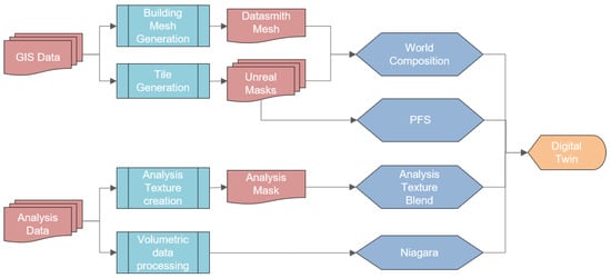
Figure 1. Combined workflow for world creation and data visualization.

3.1. World Creation

For world creation, we use GIS data provided by Lantmäteriet [53] (see Table 1), the National Department of Land Survey in Sweden, to procedurally build the natural and built environment of the selected region. For the natural environment, the features we choose for this paper are geographical features and vegetation, whereas the built environment consists of existing buildings and roads. However, this workflow can be extended to finer details of the built environment, such as road markings, traffic signage, and street furniture. We use three pre-defined processes (PPs) repeatedly throughout the world generation workflow. Figure 2 illustrates the workflow of these PPs. The PPs are used to rasterize vector GIS data and combine them into a single mosaic raster image (PP 00), subtract the buffered road networks from the raster layers (PP 01), and generate Unreal Engine-compatible tiled raster images from the previously processed mosaic (PP 02). Additionally, we use a Gaussian function to interpolate the values between two raster masks to simulate a blurring effect between them. This allows the transitions between the raster masks to appear more natural.

Table 1. Used datasets from Lantmäteriet (the National Department of Land Survey for Sweden).

Swedish Name	English Name	Description	Format
Bebyggelse	Property map	Building footprints as closed polygons	ShapeFile (*.shp)
Kommunikation	Transport networks	Transportation network as center lines	ShapeFile (*.shp)
Markdata	Land data	Land-use classification as closed polygons	ShapeFile (*.shp)
Höjddata	Elevation data	Ground elevation data as raster images	Tagged Image Format (*.TIF)
Laserdata	Laser data	LiDAR scan data as point clouds	Zipped LiDAR Aerial Survey (*.LAZ)

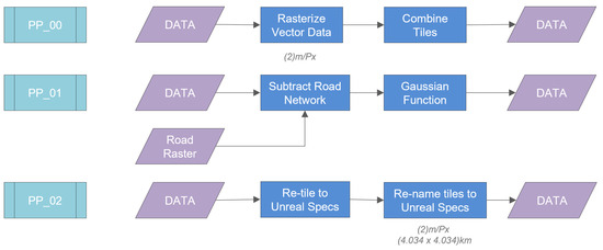
Figure 2. Pre-defined processes used in world generation workflow.

3.1.1. Terrain

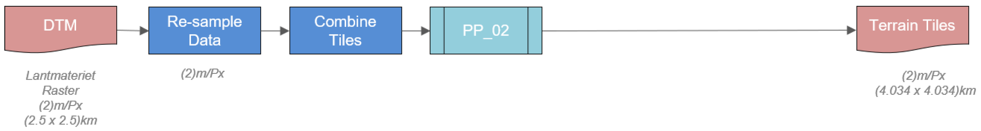
Digital terrain models (DTMs) are commonly available from most national mapping agencies. A DTM is often made available as tiled raster images, where each pixel is assigned a value representing the height of the ground at that position. In Sweden, Lantmäteriet provides a DTM at a two-meter-per-pixel resolution of 6.25 square kilometer tiles. To ensure the workflow is procedural, we introduce a post-processing step that re-samples the incoming DTM raster to a pre-determined cell spacing. The DTM is then combined into a single raster mosaic and further re-tiled into specific dimensions to ensure the maximum area while minimizing the number of tiles within the Unreal Engine (https://docs.unrealengine.com/5.0/en-US/landscape-technical-guide-in-unreal-engine/ accessed on 3 May 2023). The final step in creating the terrain tiles is to ensure the tiles are systematically named for Unreal Engine to identify the tiling layout. Once the terrain tiles are generated, they can be imported into the Unreal Engine using the World Composition feature. Figure 3 shows a flowchart of the different steps used to generate the terrain masks.

Figure 3. Workflow to generate terrain tiles.

3.1.2. Roads

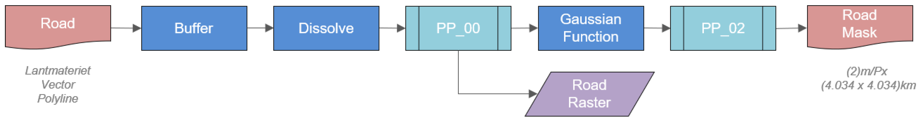
Road networks are also commonly available from national traffic authorities and are often made available as center-line data with attributes such as width, speed limit, and access. In Sweden, Lantmäteriet and Trafikverket provide road data as road center lines in the form of LineStrings or MultiLineString vector data. The vector data consist of twenty road classes, such as tunnels, thoroughfares, public roads, roads under construction, and a range of road widths for each line. We simplify the roads into four common classes with the same width and assign fixed road widths to their respective classes. The center-line data are then post-processed to form landscape masks for the Unreal Engine. First, we offset each road center line by a fixed distance to create a polygon around each line by performing a spatial buffer across all center-line polylines per road class. Then, we dissolve the resulting polygon buffer to form the road boundary regions. If there are disjointed road networks, we create multiple dissolved regions, but in most cases, a single closed region is created to form the road boundary region. We then rasterize (PP 00), tile (PP 01), and rename (PP 02) the road tiles, as shown in Figure 4.

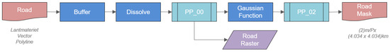
Figure 4. Workflow to generate road masks.

3.1.3. Vegetation

Lantmäteriet provides data regarding land-use classification in the form of vector polygons. The data consist of 13 natural and human-made land-use classes: water, coniferous forests, low built-up, high built-up, and industrial areas. For simplicity, we reduce the land-use classes to five: water, forest, farm, and urban. For each land-use class, the vector data are first rasterized with binary cell values (0 representing the absence of the land-use class and 1 representing its presence) to the pre-defined cell spacing as the terrain tiles. The PP of rasterizing, tiling, and renaming output tiles is carried out as shown in Figure 5. Additionally, as illustrated in Figure 1, we use the Unreal Engine Procedural Foliage System (PFS) to randomly populate instances of pre-selected foliage models such as coniferous or deciduous trees in the appropriate land-use classes.

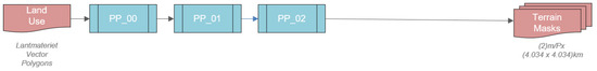
Figure 5. Workflow to generate terrain masks.

3.1.4. Buildings

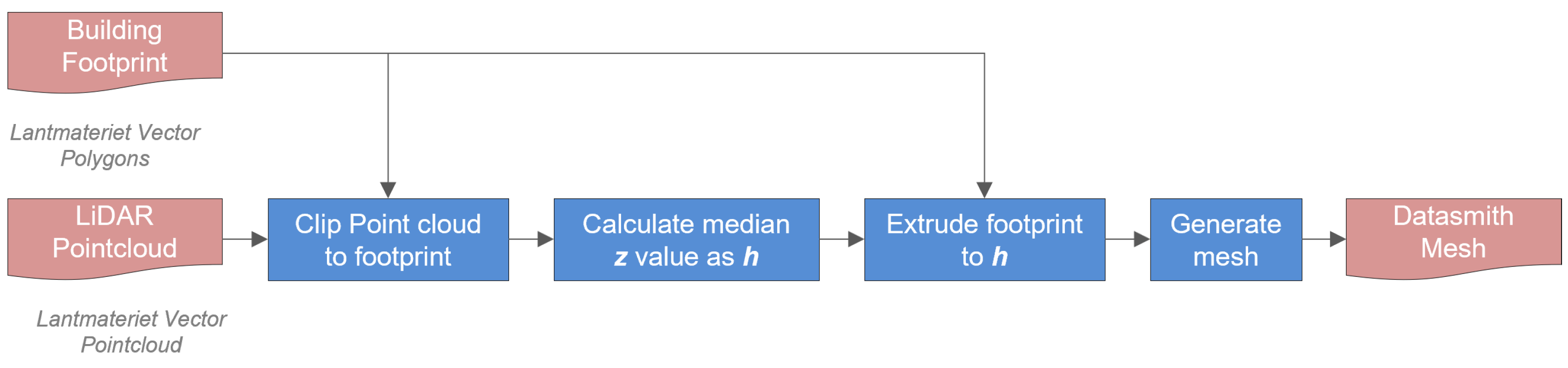
The building meshes are generated using two datasets provided by Lantmäteriet, the building footprints, and a LiDAR point cloud using the Builder platform [54]. First, we determine the mean height of the buildings by averaging the values of points in the z dimension above a building’s footprint. An LoD1 building mesh is generated by extruding the building footprints to their respective heights. The buildings are then repositioned in the z dimension to meet the terrain and generate the building mesh. The building mesh is translated to be compatible with the modified coordinate system within the Unreal Engine to align with the rest of the generated data. This mesh is then imported into the Unreal Engine, as shown in Figure 6.

Figure 6. Workflow to generate building meshes.

3.2. Unreal Engine Workflow

3.2.1. Integration of Landscape Tiles

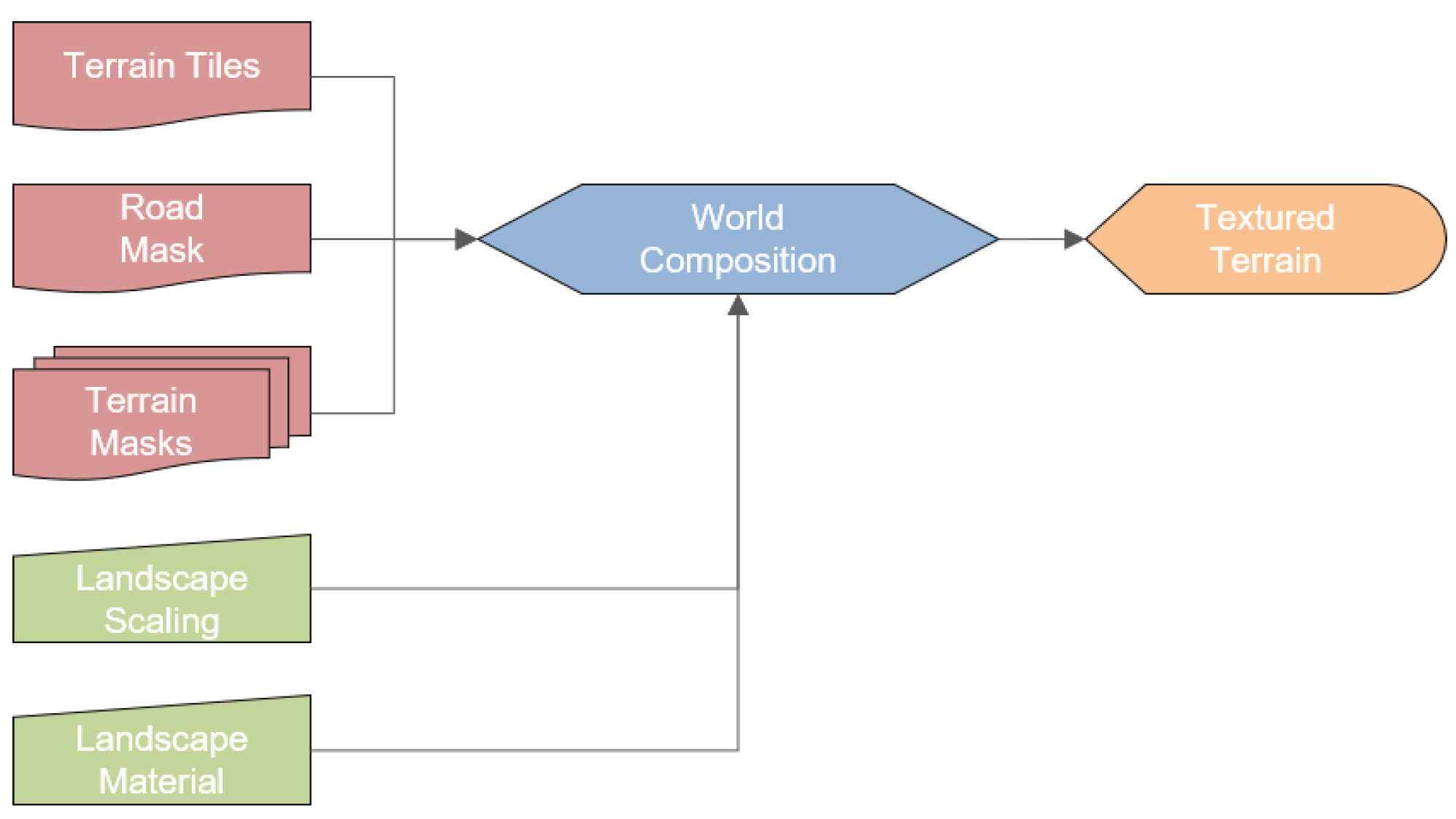
The final step in preparing the landscape tiles is to ensure that the different layers are incorporated into a seamless composition. We address two issues in this step. First, the land-use boundaries are generated irrespective of the road networks; this causes an overlap of binary raster values at the intersection of a land-use class and a road segment. Second, the process of rasterizing vector data results in a steep drop in the cell values, which are presented as pixelated boundaries at the edge of the boundaries. First, we subtract the raster data for the land-use layers with the road network to avoid any overlap; then, we apply a raster convolution filter across the layers using the Gaussian function, ensuring a gradual falloff in values at the boundaries of the layers. To complete the integration process, we import the terrain mask into the Unreal Engine using the World Composition feature, then provide the scaling factors in the x, y, and z dimensions to ensure real-world dimensions and assign the subsequent landscape masks to a procedural landscape material, as shown in Figure 7.

Figure 7. Combined workflow to generate textured terrain.

3.2.2. Procedural Landscape Material

In its material editor, Unreal Engine offers a Landscape Layer Blend feature. This feature enables us to blend together multiple textures and materials linked to the landscape masks generated in the world creation step. A layer is added for each class of landscape material (farm, forest, water, etc.), and a texture is assigned to it.

3.3. Data Visualization

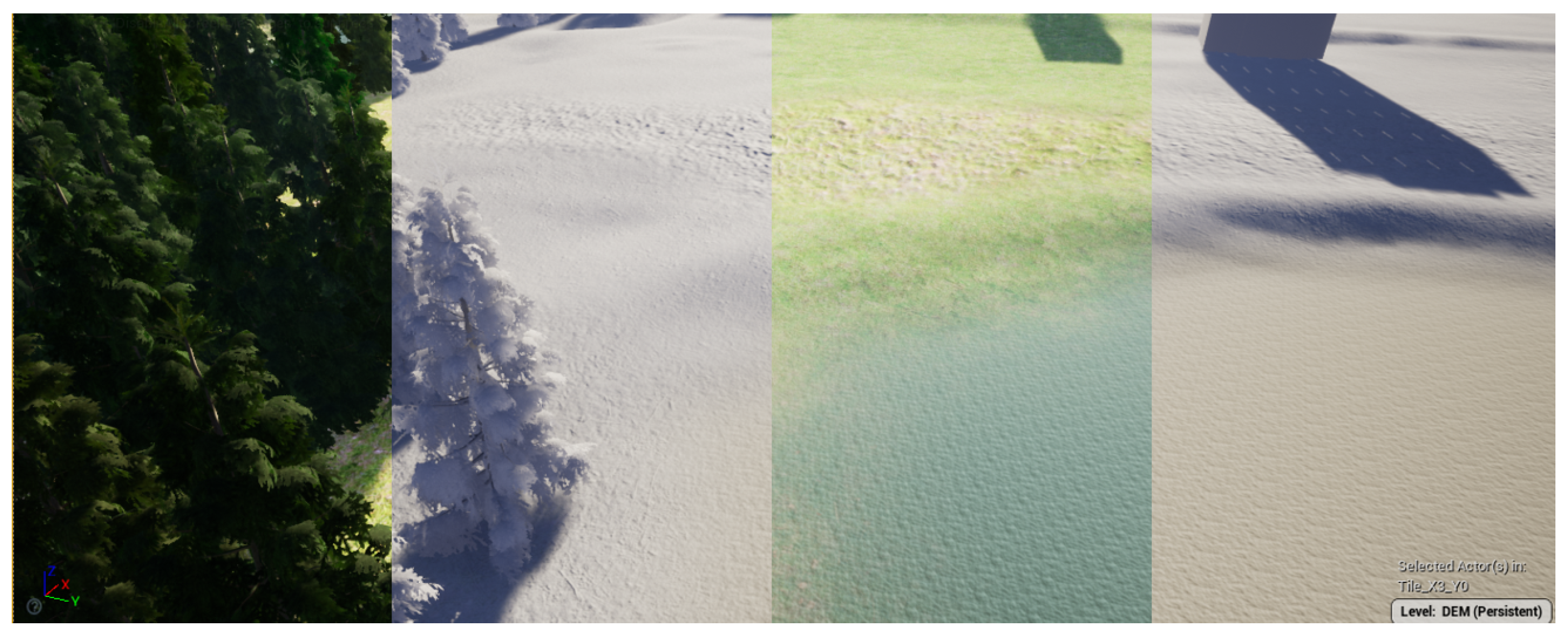
Visualization, virtual experimentation, and test-bedding are some of the key applications of VCMs [1]. The data to be visualized are produced by sensors, analysis, and simulations in various data types. The following section outlines visualization methods for isoline, volumetric, and 3D streamline data (see Figure 8). The isoline data are visualized by overlaying a scaled color value on the terrain texture. Volumetric data are visualized as volumetric particles of scaled color values, and 3D streamlines are visualized as either static or moving streamlines of particles also of a scaled color value. Urban wind simulations are conducted using the Immersed Boundary Octree Flow Solver (IBOFlow^®), previously validated for such purposes [55]. For wind comfort evaluation, historical meteorological data and local wind conditions are considered, taken from the Swedish National Weather Agency, and the expected wind speeds are statistically related to the perceived wind comfort of pedestrians. The Lawson LDDC criterion is employed for this analysis [56]. Wind data from 1961 to 2021 are sourced from the Swedish Meteorological and Hydrological Institute at Gothenburg, Sweden, at a height of 10 m above ground.

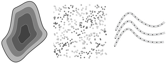
Figure 8. Illustration of the three data visualizations presented in this paper (from left to right): isoline, volumetric, and streamlines.

The simulations take into account the city’s features, such as its cityscape, vegetation, and forests, applying a Davenport–Wieringa roughness classification with a roughness length of 0.5 m. They are run in eight discrete wind directions with a reference velocity of 5 m/s in a domain that spans 1.3 km by 1.8 km, surrounded by a larger non-modeled area of 3.5 km by 3.5 km. The mesh used in the simulation contains approximately 10 million grid cells.

A novel approach is taken where the domain remains cuboidal and fixed while the geometries rotate according to the wind direction, which suits the immersed boundary method. Boundary conditions include a total pressure outlet, symmetry conditions on the domain sides and top, and standard wall functions for the ground and building surfaces.

The steady-state Reynolds-averaged Navier–Stokes equations are solved with the K-G SST model to estimate the pressure coefficient on building surfaces. This approach provides a comprehensive analysis of wind impact on urban environments, particularly assessing wind comfort for pedestrians in city settings.

The noise levels due to road traffic in the area are calculated according to local regulations, following the Nordic Prediction Method for Road Traffic Noise [43]. The model uses data on the elevation of the terrain, ground type (acoustically soft or hard), buildings and noise barriers (footprint and height), and location of road segments, with accompanying data on traffic flow (driving speed and number of light and heavy vehicles per 24 h). The model can be used to predict both 24 h-equivalent noise level and maximum noise level due to the passage of the noisiest vehicle type. Here, equivalent levels were calculated and presented as day–evening–night noise levels (Lden in dB). The indicator Lden applies a penalty on evening and night levels and is used within the EU. In the presented study, the daytime level (Lday) is also of interest, which is estimated to be 1.6 dB lower than Lden. The model is implemented in numeric code (using Matlab version r2018b and Python version 3.8) to calculate the noise level at a grid of receiver positions elevated 2 m above the ground surface, i.e., a grid noise map. Also, facade noise level calculations can be made. The ground surface model (sampled at a 2 m grid size) and built elements are provided from the developed workflow described above, whereas the road segments are imported as ShapeFiles with the traffic data as attributes. In the calculation, each road segment is divided into a set of acoustic point sources, and for each source–receiver pair, the noise level contribution is calculated following the Nordic Prediction Method (including one facade reflection), where a vertical cut plane defines the propagation condition in terms of ground profile, ground type, and shielding objects. As post-processing, the total noise level at each receiver position (grid point) is collected and exported as a CSV file for further analysis.

3.3.1. Isoline Data

Results from analyses conducted over a large area, such as noise and air quality, are available as 2D isolines from other project partners. The closed curves in the dataset represent a region with a constant value, and adjacent curves represent a fixed change in the value. The isoline data are first converted to a raster image, where we pack our data into a single grayscale image to have normalized values. We then extend the procedural landscape material to visualize data on top of the terrain, allowing us to paint pixels in certain areas that match our data. Considering that our data were packed into a single texture and each terrain tile had the same material instance applied, we introduced a custom material function in the editor that allowed us to use different data textures with various dimensions and colormaps.

First, we scaled the data texture to match the available terrain data. Then, in the material code, we accessed each pixel of the data texture and read its normalized value to map it to its respective color from the assigned color map. Next, we performed a linear interpolation between the base terrain layer (containing the existing materials of the environment, such as water, grass, and earth) and the visualized data texture, thus allowing us to display colored data on top of the terrain while showcasing the natural environment in the areas where no data were available in the data texture.

3.3.2. Volumetric Data

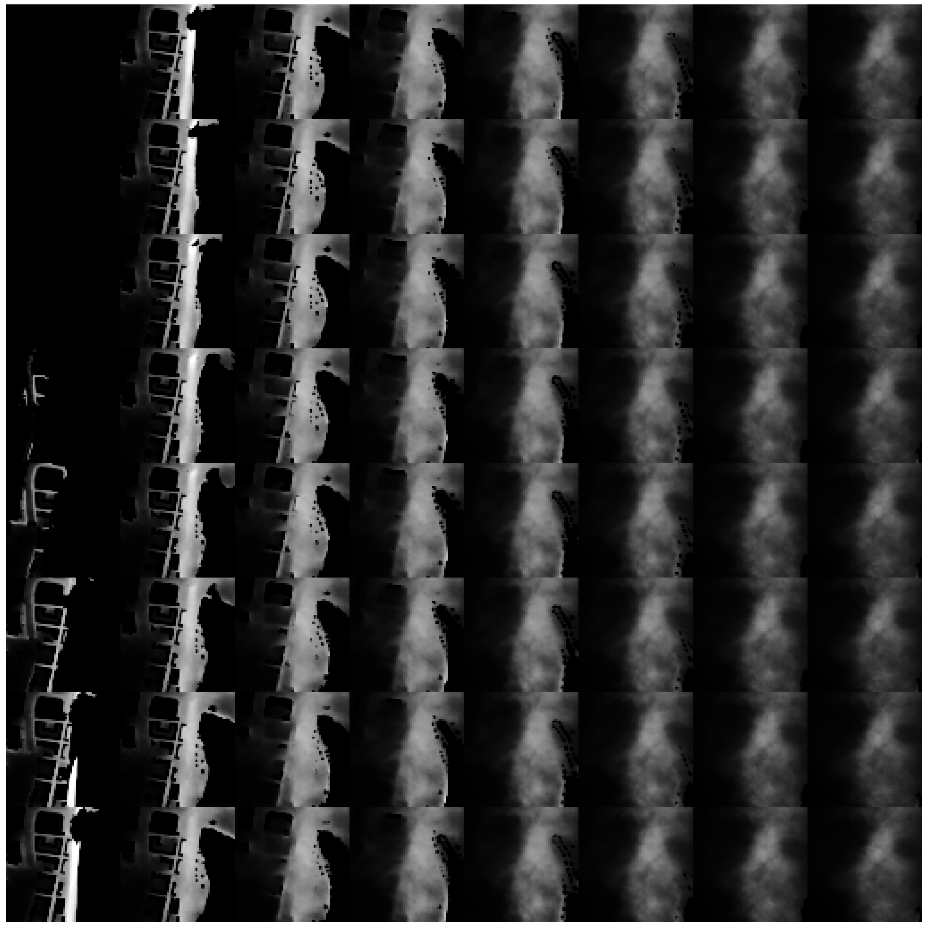
To visualize volumetric data available throughout a 3D space, such as air pollution or noise levels, we again employed the strategy of encoding the data into textures (data textures) (see Figure 9) that can be used for real-time visualization in Unreal Engine. These textures are then used to, e.g., create dynamic cut-planes using materials coded in Unreal Engine to look up the data dynamically based on the current 3D position on the surface. As these textures fold 3D data into a 2D texture, particular care must be taken to interpolate data along the z-axis (up/down in Unreal Engine). Data from the same x–y-coordinate is sampled from two places in the data texture, corresponding to the two closest z-coordinates in the data. Then, these data are interpolated to reflect the exact z-coordinate that should be sampled. The same data textures are also used as the basis for particle visualizations using the Niagara particle system in Unreal Engine, changing color, size, lifetime, etc., of particles depending on the data corresponding to the particle’s position in three dimensions.

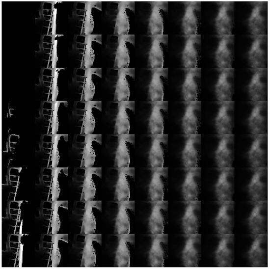
Figure 9. Data texture with 64 (8 × 8) z-levels. The contrast has been enhanced here for illustrative purposes.

The support for Python scripting in the Unreal Engine Editor provides an efficient workflow for generating the data textures. We used the experimental Python Editor Script Plugin to use the Python scripting language in Unreal Engine. Python makes it easy to read and prepare most data types using commonly available libraries, such as NumPy, and automatically imports these into native Unreal Engine Textures.

3.3.3. Particle Streamlines

We explored two different strategies for generating 3D streamlines, which show, for example, air flows in the 3D space around and between buildings.

First, we used C++ to generate procedural meshes, creating a colored tube for each 3D streamline. This visualization was high-fidelity and suitable for a limited number of static streamlines but did not allow for performant visualization of a large number of streamlines.

To enable the visualization of several thousand streamlines, we used the Niagara particle system integrated into Unreal Engine. By encoding streamlined data into data textures, as described above, the locations of streamlined segments were made accessible to the GPU using the Niagara particle system in Unreal Engine. These data generated one particle per segment of the streamlines and placed them with the correct positions and orientations to make up streamlines. With this approach, we can achieve real-time performance with 10,000+ streamlines with up to 1000 line segments per streamline, corresponding to several million line segments.

One challenge with this approach was that the position data saved into the texture needed higher precision than what is commonly used in textures for computer graphics. To properly encode the data, 32-bit textures were required. While this is supported in many key places along the pipeline (e.g., in Python and Niagara), it is not supported in the standard functions for importing textures into Unreal Engine at the time of this implementation. As such, we created and imported two 16-bit textures and merged them into one 32-bit texture using RenderTargets that currently supports 32-bit texture data. This 32-bit RenderTarget texture can be accessed directly from Niagara, providing the required data precision.

Procedural Meshed Streamlines

To create procedural streamlines, we parse the data for each streamline, a collection of points. Once we have parsed all the points for a given streamline, we generate a cylinder-like mesh around each point. The mesh generation process requires the following steps:

• Generating vertices around each parsed point of the streamline;
• Creating triangles between the generated vertices;
• Connecting sequential vertices that belong to different points.

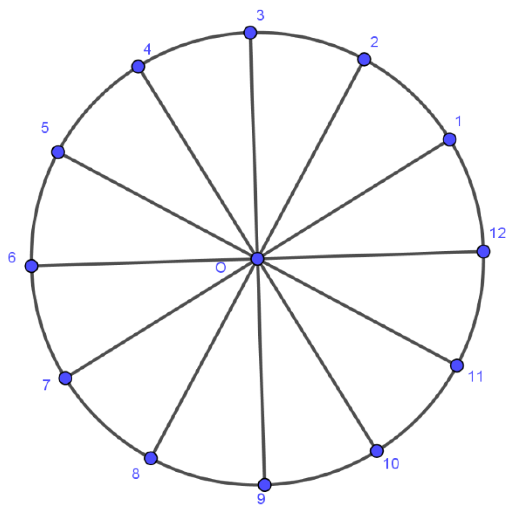
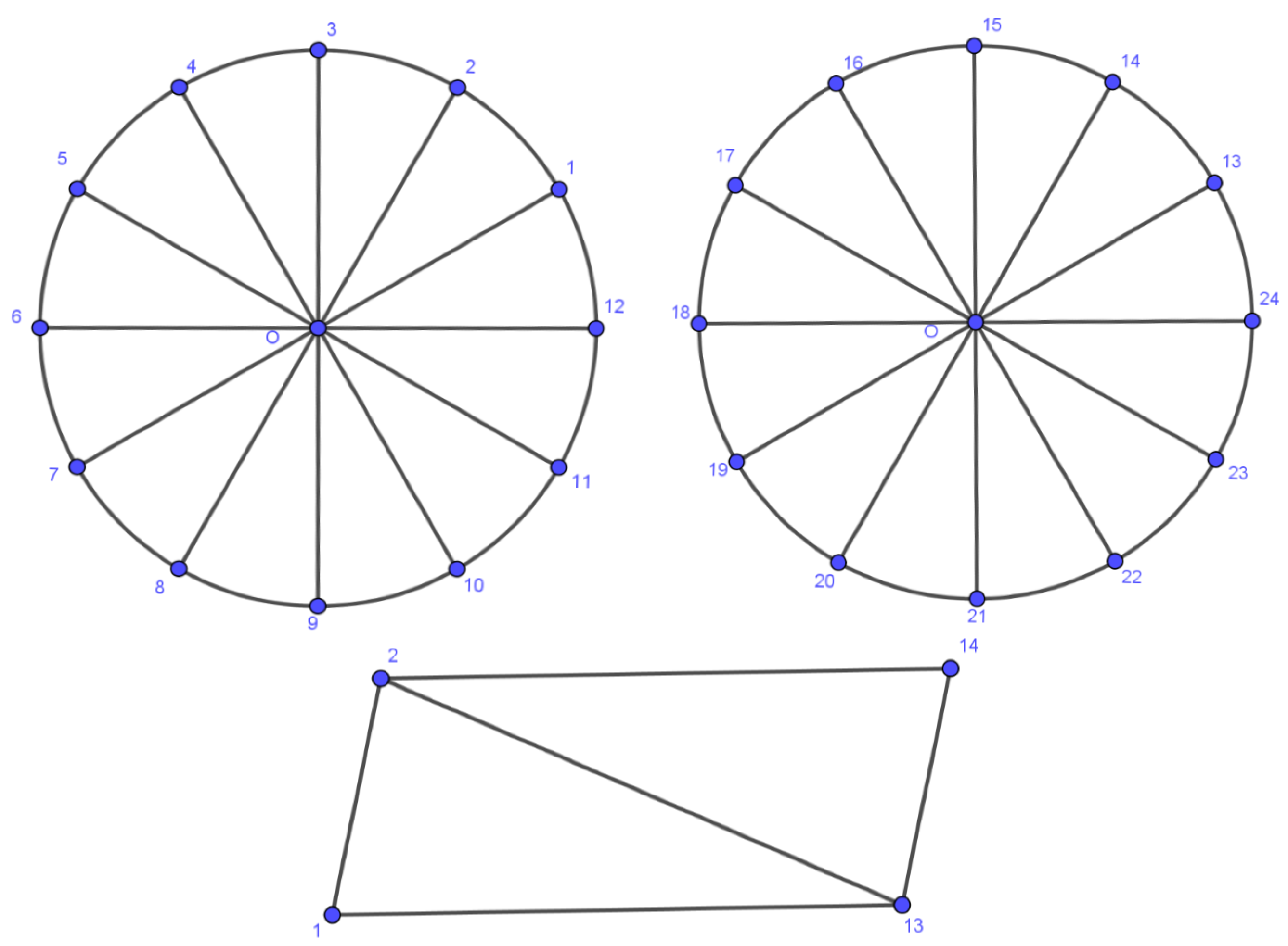
To demonstrate how the algorithm works, consider the following case. Assume that we have parsed point O from our data. As a first step, based on the description above, we need to generate vertices around that point. For that, we choose a value that can be modified in Unreal Engine, called CapVertices, which is the number of vertices that will be generated around point O. Using the polar coordinate system, we can create an initial vector $\overrightarrow{OA}$ which we are going to rotate 360/CapVertices degrees for CapVertices times around X axis to create the required vertices for the parsed point:

Once the vertices have been generated, the next step of the process is to create the required triangles to connect them. Considering Figure 10, we generate a cylinder cap for the parsed point by connecting every three vertices counterclockwise. This process is repeated for all the parsed points of a single streamline. For the mesh to look streamlined, we must connect the generated vertices belonging to different points. Figure 11 displays the generated vertices for the first and second points of a streamline, respectively. Then, to create a cylinder-like mesh between the two streamline caps, we generate a parallelogram for vertices 1, 2, 13, and 14 (displayed in the lower image section on Figure 11.

Figure 10. Generated vertices around point O.

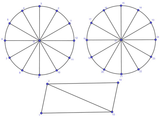
Figure 11. Upper images: Generated vertices around the first and second points of streamline. Lower image: A flattened display of connected vertices of two sequential points.

For the mesh to appear smooth and consistent, we must connect vertices 2, 13, and 1 and 2, 14, and 13 in a counterclockwise fashion. By repeating this process for all the generated vertices around all points in each streamline, we create a single cylinder-like mesh for the whole streamline.

4. Results

This section presents the results of the world creation and data visualization workflows. The results from the world creation workflow consist of asset generation using our workflow and the time required to generate and load the assets. Then, we present the results of the Unreal Engine workflow. Finally, we present the results of each visualization type—isoline data, volumetric data, and streamline data.

4.1. World Creation

World creation is the process of generating assets for Unreal Engine to consume and produce a realistic 3D representation of the real world. There are two steps to this process, generating the assets and the Unreal Engine workflow itself.

4.1.1. Generating Assets

The procedural workflow described in the Materials and Methods section is implemented in the Python programming language and designed to be easily adaptable to different data sources. It is an automated pipeline, and the only input required is the raw GIS data.

4.1.2. Unreal Engine Workflow

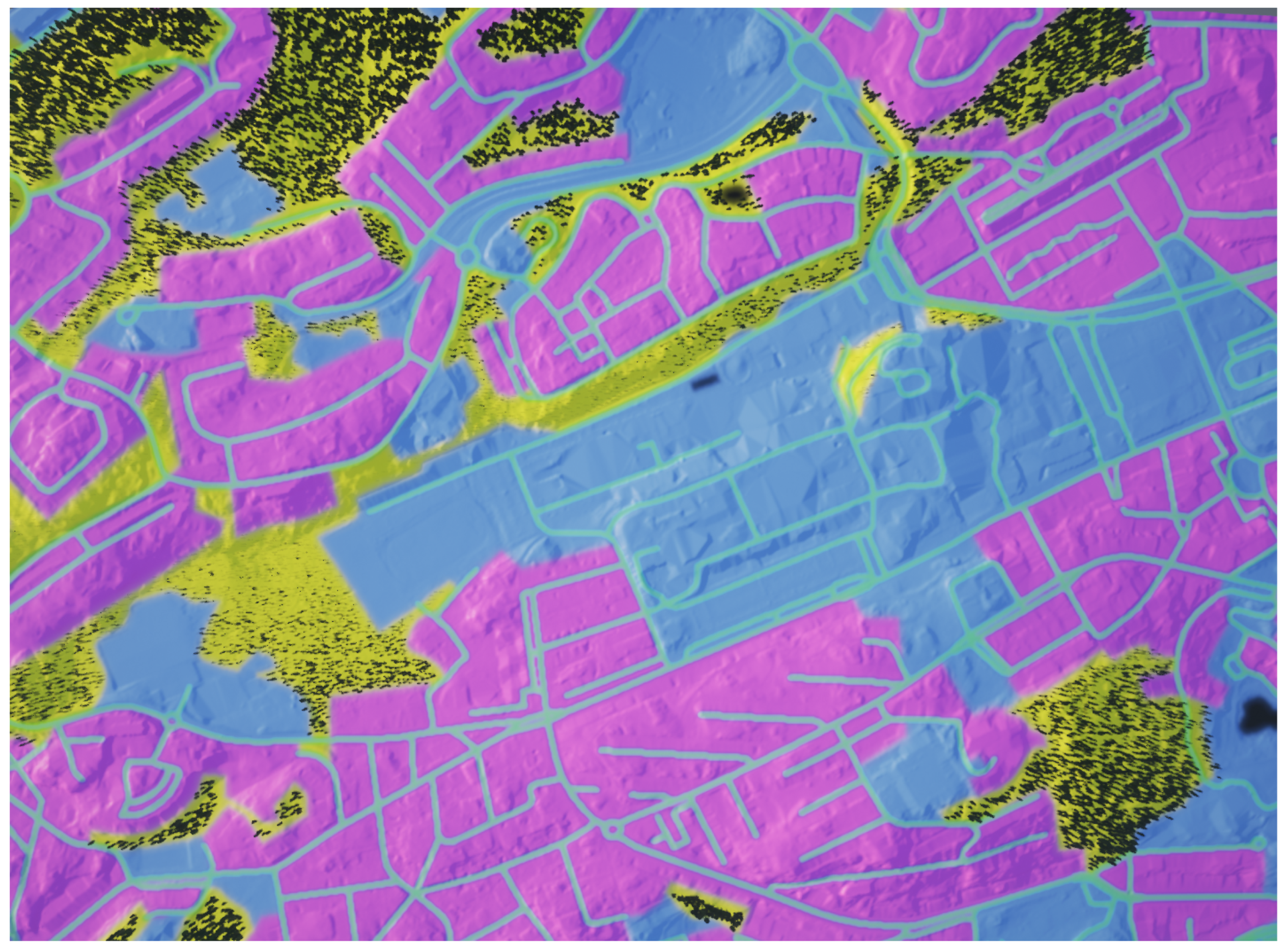
Lantmäteriet provides the data containing the boundary for each land-use category (see Figure 12). These categories include land-use types such as roads, water, forest, farm, urban, and open land. Since this information is available as vector data, it must be first converted into raster data before Unreal Engine can use it. Unreal Engine uses these black and white masks as raster images to identify where the different materials must be applied within the 3D model (black representing the absence of a category and white representing the presence of it). One of the problems we encounter in this process is the interaction between the different land-use types at the edges of the boundary. The edges are sharp and do not blend into one another naturally. The final image with the blended materials overlaid with simulation data is shown in Figure 13.

Figure 12. Aerial view of terrain model with landscape masks applied—Unreal Engine. The colours represent different land use regions.

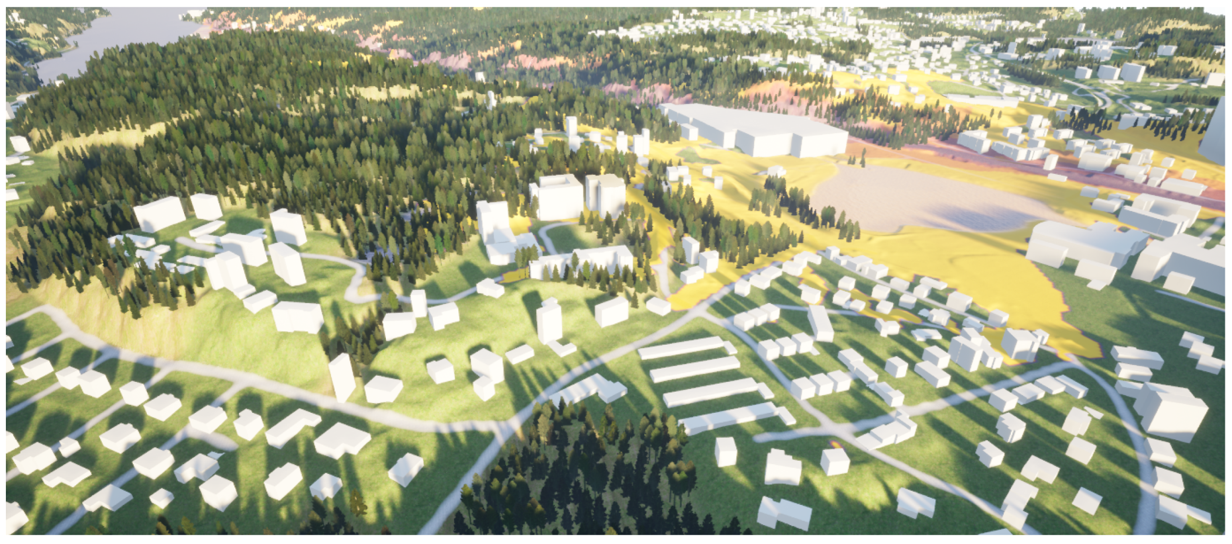
Figure 13. Aerial view of the final 3D model—Unreal Engine.

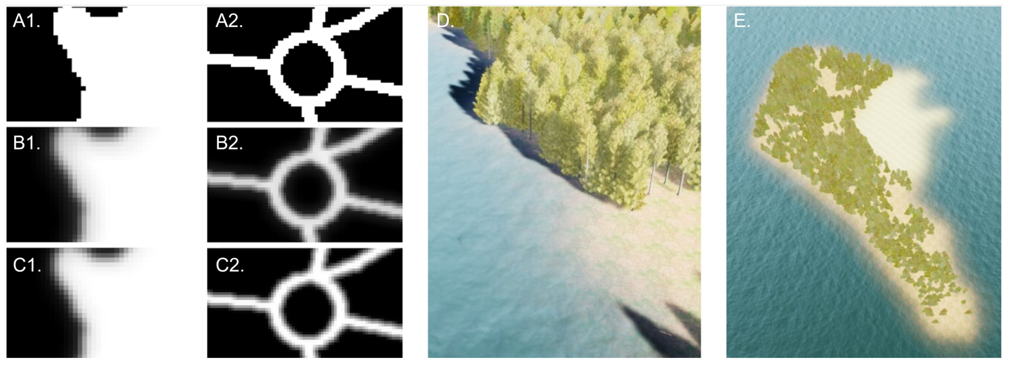
We use a Gaussian function to smooth the edges naturally to solve this. The softening of the edges is achieved using convolution, where a matrix operation is performed on an array of pixels according to a set of pre-defined weights. Figure 14(A1,A2) show a land-use mask for a region containing forests and roads, respectively, with no filtering. Figure 14B,C show the results of different weights provided to the Gaussian function. Figure 14D,E show the results of the layer blending once the processed masks are loaded into Unreal Engine.

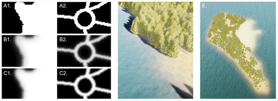
Figure 14. (A1–C1,A2–C2) Results of convolution filters on the landscape masks. (D,E) Result of convolution on landscape masks—Unreal Engine.

Combining multiple layers allows adding a level of detail to the geometry without increasing the complexity of the 3D model. This is achieved by layering specific textures that inform Unreal Engine on how light interacts with these materials. Figure 15 shows an image from the final model with the diffuse colors turned on and off. In the sections where the colors are turned off, we see fine details on the ground that vary depending on the land-use type. These details are created using bump and displacement textures that contain information on how the smooth terrain can be distorted to provide natural imperfections to the model without requiring additional polygons. The buildings are loaded into Unreal Engine as LoD1 building meshes and aligned to their coordinate position (see Figure 16).

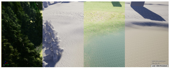
Figure 15. Composition of material details in the 3D model—Unreal Engine.

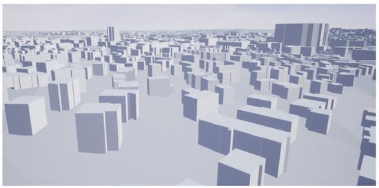
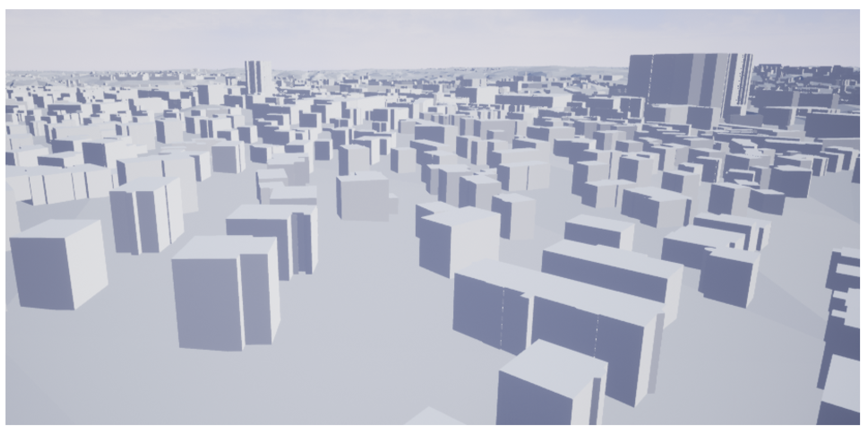
Figure 16. LoD1 meshes within Unreal Engine.

4.2. Data Visualization

Once the 3D representation of the world is achieved, DTs must also be able to visualize various data types resulting from urban simulations like CFD and noise studies. In this section, we outline three common result data types that are visualized in DTs, isoline, volumetric and streamline data, with examples provided for each.

4.2.1. Isoline Data

A dataset containing the results of a noise simulation for a region was used to illustrate the visualization of isoline data. The dataset contains vector data in the form of polygons representing different intensities of noise levels. The vector data are encoded into a 2D texture. The 2D texture is then remapped within Unreal Engine to a color scale selected by the user and draped over the landscape. Figure 17 shows the results of visualizing the isoline data.

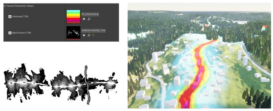
Figure 17. (Left, top) Unreal Engine user interface for loading the color scale image and the grayscale mask of data to be visualized. (Left, bottom) Grayscale mask to be visualized. (Right) Final visualization of grayscale mask—Unreal Engine.

4.2.2. Volumetric Data

A dataset covering a volume of 512 × 512 × 64 was encoded into a data texture by folding the z-coordinate into an 8 × 8 grid in a 2D texture. This requires the total resolution of the texture to be (512 × 8) × (512 × 8) = 4196 × 4196. The calculations required to look up the data in this texture are performed directly in the Niagara particle system module, which can run on the GPU. Particles can be spawned and placed within this volume in several ways, but we primarily spawn particles randomly within the volume and kill them if they are, e.g., below a set threshold value (see Figure 18). This approach makes it easy to vary the number of particles used to visualize the data depending on performance requirements.

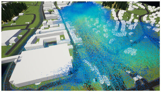
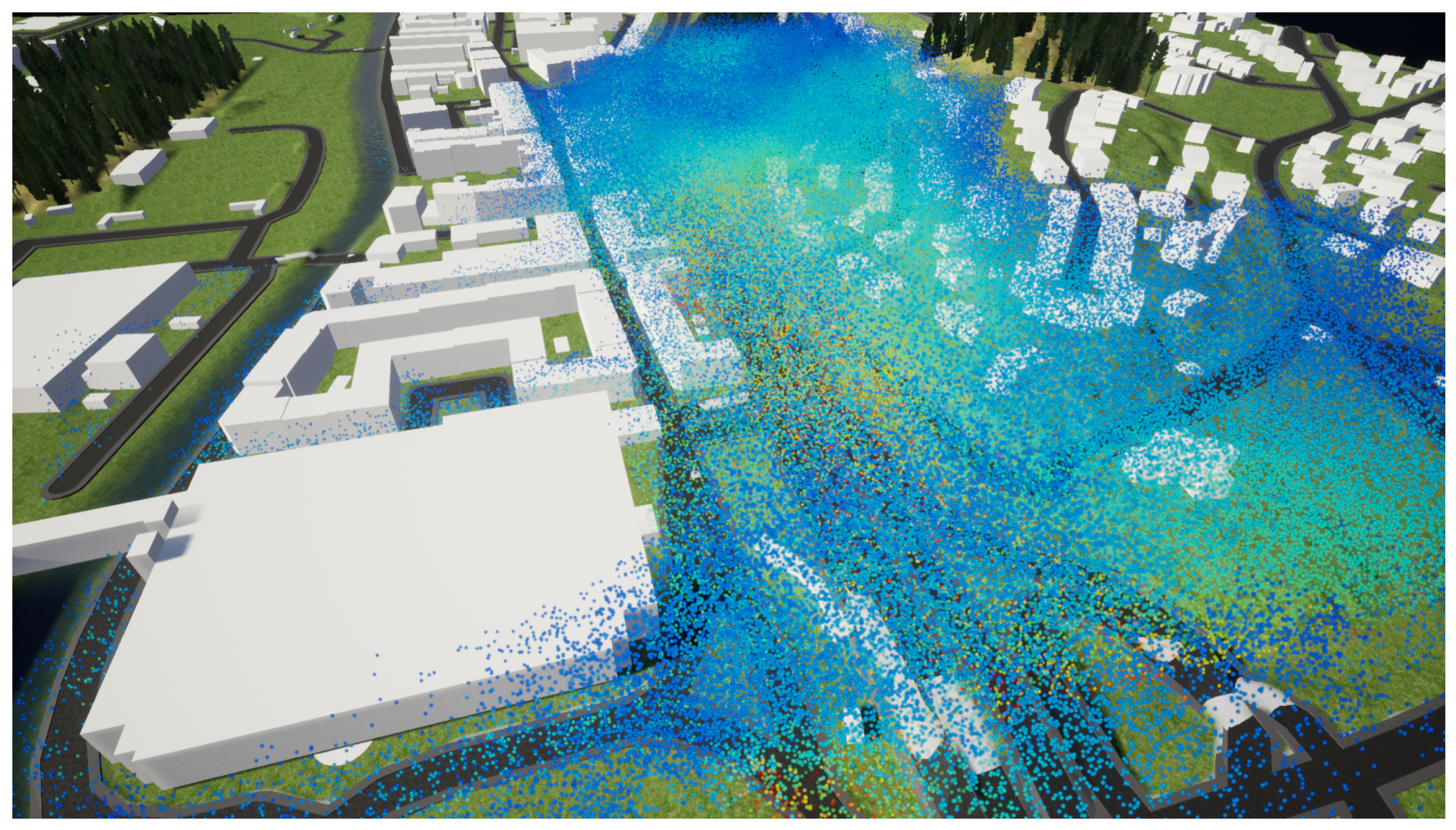
Figure 18. Volumetric data visualized with particles on top of generated building and terrain geometry. With up to 2 million particles, colored to show NO₂ concentration and moving to visualize wind. The median frame time is 7 ms, with approximately 5 ms for the environment and 2 ms for the particle visualization.

4.2.3. Streamlines

Any vector flow data can be visualized as 3D streamlines, where each streamline is a representation of the path a vector field takes. The components of a streamline are a vector and a magnitude at a resolved interval. In the case of CFD data, streamlines can show the direction and path of the wind along with the intensity of wind speed. It is also desirable to interpolate along the streamline to show the magnitude variation along the path the wind is moving in.

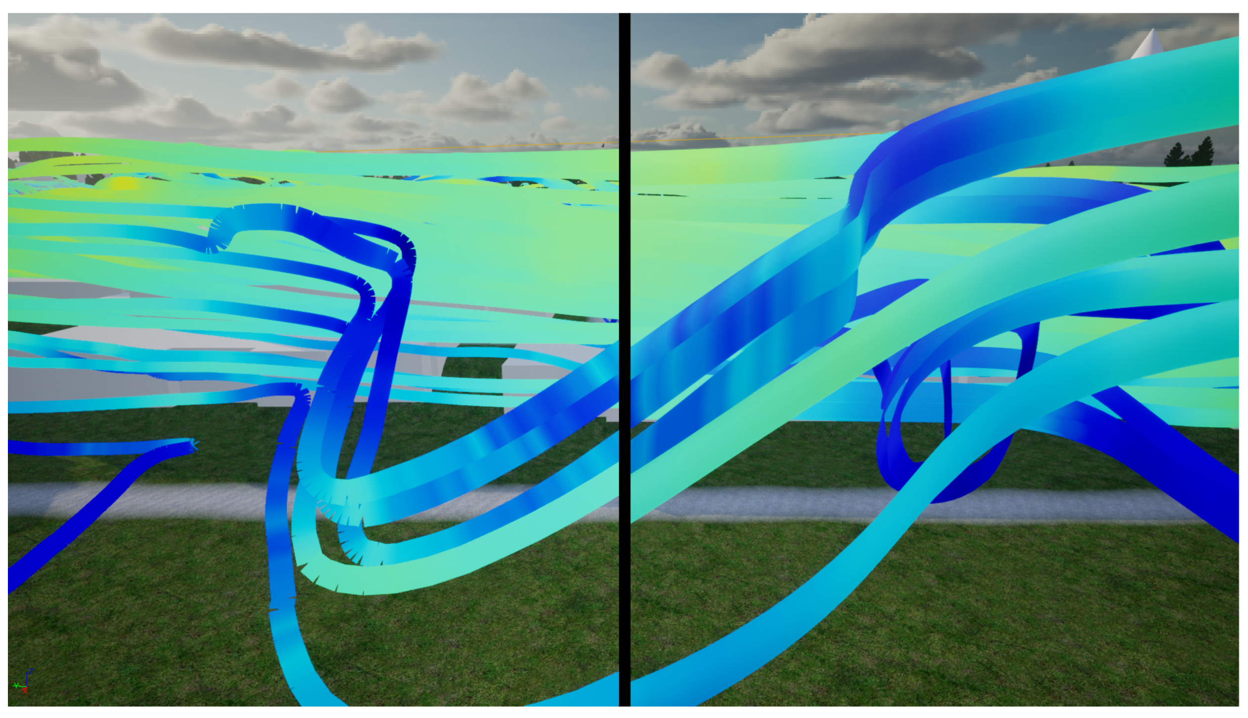
Procedurally generated streamlines and particle streamlines have complementary values, as procedurally generated streamlines have higher visual quality up close, but particle streamlines perform better with many streamlines. Figure 19 shows an overview at a distance where it is not possible to tell the difference visually. Here, it would generally be preferable to use particle streamlines. Figure 20 shows a close-up comparison, where artifacts can be seen in the sharp turns of particle streamlines to the left. Table 2 lists performance numbers for the two options with different numbers of streamlines.

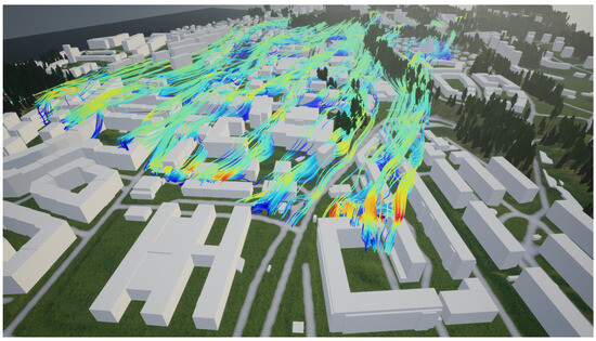
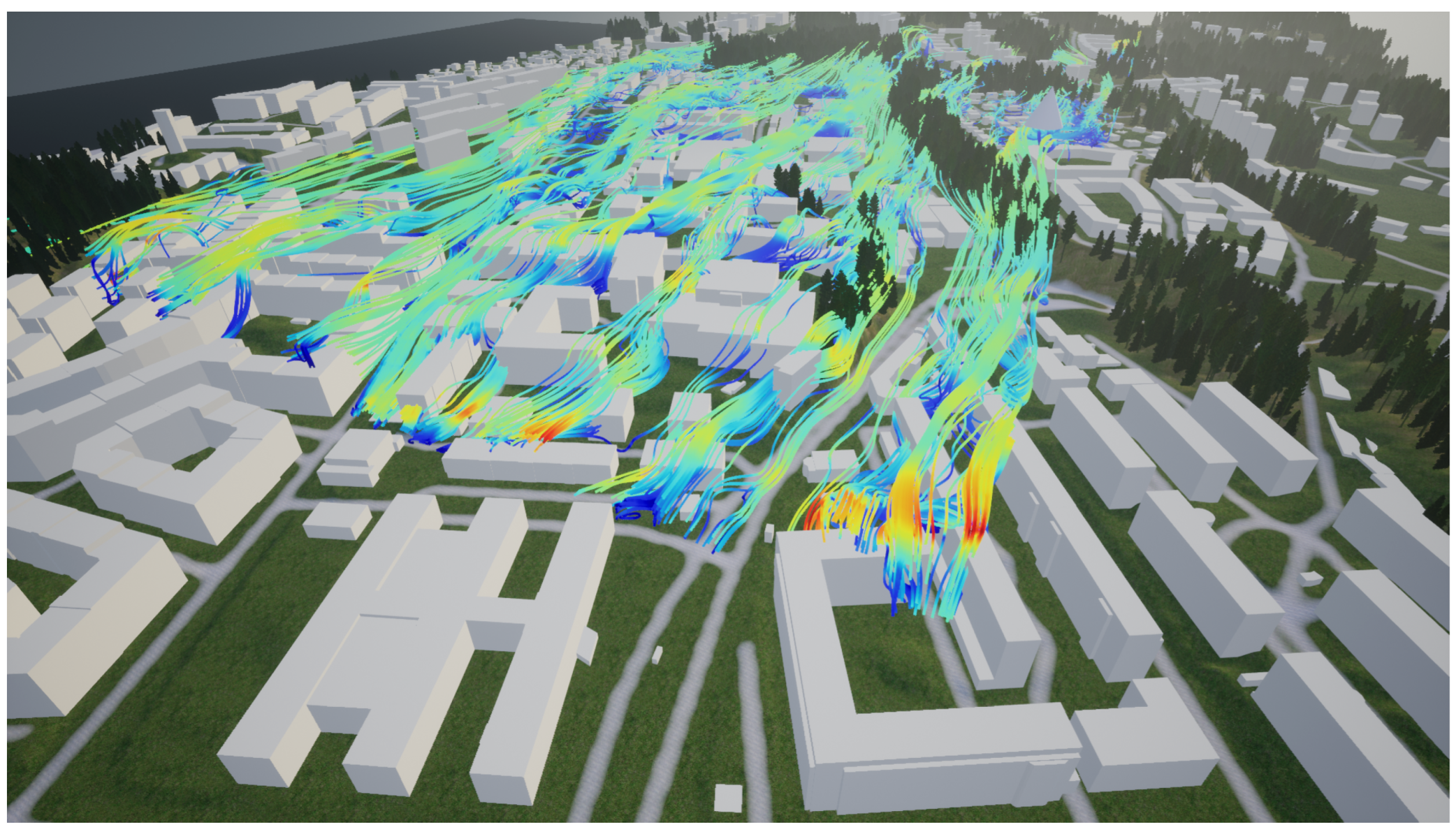
Figure 19. Streamlines overview showing 1003 (from a specific dataset) streamlines over generated building and landscape geometry.

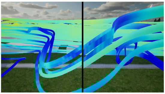
Figure 20. Streamlines comparison. (Left) displays the particle system implementation and (Right) streamlines with the procedural mesh.

Table 2. Comparison of performance of procedural streamlines and particle streamlines, with different numbers of streamlines. Median frame timings over 15 s on Nvidia GeForce RTX 2080 Ti. (Nvidia Corporation, Santa Clara, CA, USA).

Streamlines Number	Procedural Streamlines	Particle Streamlines
1003	12 ms	5 ms
4158	47 ms	12 ms
8316	134 ms	51 ms
12,474	247 ms	127 ms

5. Limitations and Discussion

The results of the proposed workflow show how a realistic virtual city model can be generated and how large-scale data can be visualized efficiently and accurately for various data types. One of the main advantages of our proposed workflow is that it allows decision-makers to view alternate scenarios, both real and simulated, to make well-informed decisions. For instance, decision-makers can use the resulting virtual city model to test different traffic scenarios and assess air pollution or noise levels resulting from a new construction project. In comparison to techniques previously described in the literature, the aim of this paper was to combine data acquisition pipelines with reproducible and procedural workflows that anyone can access. Our methods do not explicitly require access to any proprietary software or datasets and can be implemented on almost all modern personal computers.

Our workflow’s final output is a visual representation of the real world. Like any representative technique, our methods use different levels of abstraction to simplify this process. As such, a “validation” of this process goes beyond the technical details of implementation. While there is significant literature on visualizing scientific data, such as simulation results, validating the visual quality of the digital twin can be highly subjective. It depends on the context in which the visualization is presented, the audience, and, most importantly, the intent of the communication. While the scope of the paper is limited to the technical description of the methods, we point readers interested in the qualitative validation of our methods to [57], where we conducted user studies in real-world scenarios with stakeholders to gather feedback on their subjective experiences within the 3D environments generated through our methods in virtual reality.

The proposed workflow is not intended to be an absolute solution for creating DTs; rather, it is a starting point on which further research can build. The steps for a complete, end-to-end solution involve developing robust systems for building detection, rooftop recognition, and geometry generation and importing and visualizing data in the same 3D environment. The workflow may be enriched by adding new semantic categories for land-use types. With developments in artificial intelligence and computer vision, it may be possible to identify additional LoD elements from the urban environment, such as roofs [58,59], facade details [60,61], and the positions of park benches, street lights, and other urban furniture. New real-time data sources may also be visualized, such as dynamic positions of public transport systems, cars, and pedestrian flows. The landscape of real-time game engines such as Unity and Unreal Engine is developing at a rapid pace; the main bottlenecks to achieving higher accuracy and detail lie in the quality and availability of data sources. As new data sources become more readily available, the workflow can be adapted to cover new data types to be visualized.

With developments in communication systems and cloud-based computing, it is also now becoming possible to run complex real-time multi-domain urban simulations such as noise, radiation, energy, and wind [62] and optimize the architectural design variables [63] to improve the sustainability of cities [64]. The preliminary data types supported by our workflow should be sufficient in the near future to support the visualization results from any such simulations.

However, there are limitations to the proposed method. Spatial data is often not available in all regions and, when available, may not be of high quality. Additionally, spatial data may use several different coordinate reference systems, which are generally not natively supported by software like Unreal Engine. This necessitates manually aligning meshes such as buildings and terrain with data visualizations and analysis layers, leading to inconsistencies. Another limitation is the significant computational resources and expertise in GIS and game development required. Moreover, maintaining and updating digital twins of cities demands constant integration of extensive and dynamic data from multiple sources to accurately represent the evolving urban landscape [65]. Our proposed workflow does not address these complexities despite the importance of a synchronous digital twin [66]. The methods presented are limited to the procedural creation of virtual 3D environments as a base for an urban digital twin system. Currently, the workflow supports only static data visualization, and further research is necessary to enable simulations within a digital twin and the visualization of large-scale, real-time urban data.

6. Conclusions

Generating virtual environments that represent the physical world is time-consuming and often complex. This paper presents a workflow for the procedural generation of such virtual worlds using commonly available GIS datasets enabled through modern game engines like Unreal Engine. In addition to generating virtual worlds, we present workflows to visualize data from large-scale analysis of the built environment in raster and vector formats. The methods presented in the paper can be elaborated to include a greater level of detail, such as the number of land-use classes included in the model, increasing the points in the material and texture composition, and increasing the level of detail in the building meshes.

For researchers interested in building on these techniques, we suggest further investigating how to efficiently visualize real-time sensor data from IoT sensors and how can visualization techniques developed within the game development industry be carried over into the research and development of urban digital twins. We point readers to open-source work on visualizing sensor data by developers at the consulting firm WSP (https://github.com/Azure-Samples/azure-digital-twins-unreal-integration (accessed on 20 May 2024)) as a practical starting point. We also encourage researchers to conduct empirical user studies to evaluate the effectiveness of visualization techniques in urban DTs for different types of data sources (see [67]). The role of LoDs in communicating scenarios of planning and redevelopment through DTs is another interesting research direction to pursue, building on research from the fields of architecture and urban planning. While the exploration of multi-domain urban simulations was not within the scope of this paper, it offers an under-explored research area for DTs. Urban simulations are often carried out in silos by domain experts; researchers can investigate what additional value DTs may offer and how these results may be communicated to decision-makers effectively (see [62]).

In conclusion, the workflow presented in this paper shows an innovative approach to creating 3D virtual city models, visualizing large-scale urban data using GIS, and leveraging the advances in real-time game engines like Unreal Engine. Viewing urban data in a realistic context can help decision-makers make more informed decisions. However, our workflow requires significant computational resources and expertise, and the availability and accuracy of GIS data needed for this workflow may be a limiting factor.

7. Declaration of AI in the Writing Process

While preparing this work, the author(s) used ChatGPT to rewrite parts of the text. After using this tool/service, the author(s) reviewed and edited the content as needed and take(s) full responsibility for the publication’s content.

References

- Ketzler, B.; Naserentin, V.; Latino, F.; Zangelidis, C.; Thuvander, L.; Logg, A. Digital Twins for Cities: A State of the Art Review. Built Environ. 2020, 46, 547–573. [Google Scholar] [CrossRef]
- Gil, J. City Information Modelling: A Conceptual Framework for Research and Practice in Digital Urban Planning. Built Environ. 2020, 46, 501–527. [Google Scholar] [CrossRef]
- Logg, A.; Mardal, K.A.; Wells, G. Automated Solution of Differential Equations by the Finite Element Method: The FEniCS Book; Springer Science & Business Media: Berlin/Heidelberg, Germany, 2012; Volume 84. [Google Scholar]
- Girindran, R.; Boyd, D.S.; Rosser, J.; Vijayan, D.; Long, G.; Robinson, D. On the Reliable Generation of 3D City Models from Open Data. Urban Sci. 2020, 4, 47. [Google Scholar] [CrossRef]
- Pađen, I.; García-Sánchez, C.; Ledoux, H. Towards automatic reconstruction of 3D city models tailored for urban flow simulations. Front. Built Environ. 2022, 8, 899332. [Google Scholar] [CrossRef]
- Ledoux, H.; Biljecki, F.; Dukai, B.; Kumar, K.; Peters, R.; Stoter, J.; Commandeur, T. 3dfier: Automatic reconstruction of 3D city models. J. Open Source Softw. 2021, 6, 2866. [Google Scholar] [CrossRef]
- Batty, M. Digital twins. Environ. Plan. Urban Anal. City Sci. 2018, 45, 817–820. [Google Scholar] [CrossRef]
- Ham, Y.; Kim, J. Participatory sensing and digital twin city: Updating virtual city models for enhanced risk-informed decision-making. J. Manag. Eng. 2020, 36, 04020005. [Google Scholar] [CrossRef]
- Latino, F.; Naserentin, V.; Öhrn, E.; Shengdong, Z.; Fjeld, M.; Thuvander, L.; Logg, A. Virtual City@ Chalmers: Creating a prototype for a collaborative early stage urban planning AR application. Proc. eCAADe RIS 2019, 137–147. Available online: https://www.researchgate.net/profile/Fabio-Latino/publication/333134046_Virtual_CityChalmers_Creating_a_prototype_for_a_collaborative_early_stage_urban_planning_AR_application/links/5cdd4e62299bf14d959d0cb7/Virtual-CityChalmers-Creating-a-prototype-for-a-collaborative-early-stage-urban-planning-AR-application.pdf (accessed on 19 March 2024).
- Muñumer Herrero, E.; Ellul, C.; Cavazzi, S. Exploring Existing 3D Reconstruction Tools for the Generation of 3D City Models at Various Lod from a Single Data Source. ISPRS Ann. Photogramm. Remote Sens. Spat. Inf. Sci. 2022, X-4/W2, 209–216. [Google Scholar] [CrossRef]
- Nan, L.; Wonka, P. PolyFit: Polygonal Surface Reconstruction From Point Clouds. In Proceedings of the IEEE International Conference on Computer Vision, Venice, Italy, 22–29 October 2017; pp. 2353–2361. [Google Scholar]
- Poux, F. 5-Step Guide to Generate 3D Meshes from Point Clouds with Python. 2021. Available online: https://towardsdatascience.com/5-step-guide-to-generate-3d-meshes-from-point-clouds-with-python-36bad397d8ba (accessed on 3 May 2023).
- Schnabel, R.; Wahl, R.; Klein, R. Efficient RANSAC for Point-Cloud Shape Detection. Comput. Graph. Forum 2007, 26, 214–226. [Google Scholar] [CrossRef]
- Wang, H. Design of Commercial Building Complex Based on 3D Landscape Interaction. Sci. Program. 2022, 2022, 7664803. [Google Scholar] [CrossRef]
- Coors, V.; Betz, M.; Duminil, E. A Concept of Quality Management of 3D City Models Supporting Application-Specific Requirements. PFG J. Photogramm. Remote Sens. Geoinf. Sci. 2020, 88, 3–14. [Google Scholar] [CrossRef]
- García-Sánchez, C.; Vitalis, S.; Paden, I.; Stoter, J. The impact of level of detail in 3D city models for cfd-based wind flow simulations. Int. Arch. Photogramm. Remote Sens. Spat. Inf. Sci. 2021, XLVI-4/W4-2021, 67–72. [Google Scholar] [CrossRef]
- Deininger, M.E.; von der Grün, M.; Piepereit, R.; Schneider, S.; Santhanavanich, T.; Coors, V.; Voß, U. A Continuous, Semi-Automated Workflow: From 3D City Models with Geometric Optimization and CFD Simulations to Visualization of Wind in an Urban Environment. ISPRS Int. J. Geo-Inf. 2020, 9, 657. [Google Scholar] [CrossRef]
- Kolbe, T.H.; Donaubauer, A. Semantic 3D City Modeling and BIM. In Urban Informatics; Shi, W., Goodchild, M.F., Batty, M., Kwan, M.P., Zhang, A., Eds.; The Urban Book Series; Springer: Singapore, 2021; pp. 609–636. [Google Scholar] [CrossRef]
- Dimitrov, H.; Petrova-Antonova, D. 3D city model as a first step towards digital twin of Sofia city. Int. Arch. Photogramm. Remote Sens. Spat. Inf. Sci. 2021, 43, 23–30. [Google Scholar] [CrossRef]
- Singla, J.G.; Padia, K. A Novel Approach for Generation and Visualization of Virtual 3D City Model Using Open Source Libraries. J. Indian Soc. Remote Sens. 2021, 49, 1239–1244. [Google Scholar] [CrossRef]
- OpenStreetMap Contributors. OpenStreetMap. 2024. Available online: https://www.openstreetmap.org (accessed on 22 May 2024).
- Pepe, M.; Costantino, D.; Alfio, V.S.; Vozza, G.; Cartellino, E. A Novel Method Based on Deep Learning, GIS and Geomatics Software for Building a 3D City Model from VHR Satellite Stereo Imagery. ISPRS Int. J. Geo-Inf. 2021, 10, 697. [Google Scholar] [CrossRef]
- Buyukdemircioglu, M.; Kocaman, S. Reconstruction and Efficient Visualization of Heterogeneous 3D City Models. Remote Sens. 2020, 12, 2128. [Google Scholar] [CrossRef]
- Döllner, J.; Buchholz, H. Continuous Level-of-Detail Modeling of Buildings in 3D City Models. In Proceedings of the 13th Annual ACM International Workshop on Geographic Information Systems, GIS ’05, Bremen, Germany, 4–5 November 2005; pp. 173–181. [Google Scholar] [CrossRef]
- Ortega, S.; Santana, J.M.; Wendel, J.; Trujillo, A.; Murshed, S.M. Generating 3D City Models from Open LiDAR Point Clouds: Advancing Towards Smart City Applications. In Open Source Geospatial Science for Urban Studies: The Value of Open Geospatial Data; Mobasheri, A., Ed.; Lecture Notes in Intelligent Transportation and Infrastructure; Springer International Publishing: Cham, Switzerland, 2021; pp. 97–116. [Google Scholar] [CrossRef]
- Katal, A.; Mortezazadeh, M.; Wang, L.L.; Yu, H. Urban Building Energy and Microclimate Modeling–From 3D City Generation to Dynamic Simulations. Energy 2022, 251, 123817. [Google Scholar] [CrossRef]
- Peters, R.; Dukai, B.; Vitalis, S.; van Liempt, J.; Stoter, J. Automated 3D reconstruction of LoD2 and LoD1 models for all 10 million buildings of the Netherlands. Photogramm. Eng. Remote Sens. 2022, 88, 165–170. [Google Scholar] [CrossRef]
- Alomía, G.; Loaiza, D.; Zúñiga, C.; Luo, X.; Asoreycacheda, R. Procedural modeling applied to the 3D city model of bogota: A case study. Virtual Real. Intell. Hardw. 2021, 3, 423–433. [Google Scholar] [CrossRef]
- Chen, Z.; Ledoux, H.; Khademi, S.; Nan, L. Reconstructing Compact Building Models from Point Clouds Using Deep Implicit Fields. ISPRS J. Photogramm. Remote Sens. 2022, 194, 58–73. [Google Scholar] [CrossRef]
- Diakite, A.; Ng, L.; Barton, J.; Rigby, M.; Williams, K.; Barr, S.; Zlatanova, S. Liveable City Digital Twin: A Pilot Project for the City of Liverpool (nsw, Australia). ISPRS Ann. Photogramm. Remote Sens. Spat. Inf. Sci. 2022, 10, 45–52. [Google Scholar] [CrossRef]
- Biljecki, F.; Stoter, J.; Ledoux, H.; Zlatanova, S.; Çöltekin, A. Applications of 3D city models: State of the art review. ISPRS Int. J. Geo-Inf. 2015, 4, 2842–2889. [Google Scholar] [CrossRef]
- Fuller, A.; Fan, Z.; Day, C.; Barlow, C. Digital twin: Enabling technologies, challenges and open research. IEEE Access 2020, 8, 108952–108971. [Google Scholar] [CrossRef]
- Lei, B.; Janssen, P.; Stoter, J.; Biljecki, F. Challenges of urban digital twins: A systematic review and a Delphi expert survey. Autom. Constr. 2023, 147, 104716. [Google Scholar] [CrossRef]
- Yu, J.; Stettler, M.E.; Angeloudis, P.; Hu, S.; Chen, X.M. Urban network-wide traffic speed estimation with massive ride-sourcing GPS traces. Transp. Res. Part Emerg. Technol. 2020, 112, 136–152. [Google Scholar] [CrossRef]
- Chen, B.; Xu, B.; Gong, P. Mapping essential urban land use categories (EULUC) using geospatial big data: Progress, challenges, and opportunities. Big Earth Data 2021, 5, 410–441. [Google Scholar] [CrossRef]
- Ferré-Bigorra, J.; Casals, M.; Gangolells, M. The adoption of urban digital twins. Cities 2022, 131, 103905. [Google Scholar] [CrossRef]
- Dembski, F.; Wössner, U.; Letzgus, M.; Ruddat, M.; Yamu, C. Urban digital twins for smart cities and citizens: The case study of Herrenberg, Germany. Sustainability 2020, 12, 2307. [Google Scholar] [CrossRef]
- Shahat, E.; Hyun, C.T.; Yeom, C. City digital twin potentials: A review and research agenda. Sustainability 2021, 13, 3386. [Google Scholar] [CrossRef]
- Mylonas, G.; Kalogeras, A.; Kalogeras, G.; Anagnostopoulos, C.; Alexakos, C.; Muñoz, L. Digital twins from smart manufacturing to smart cities: A survey. IEEE Access 2021, 9, 143222–143249. [Google Scholar] [CrossRef]
- Jeddoub, I.; Nys, G.A.; Hajji, R.; Billen, R. Digital Twins for cities: Analyzing the gap between concepts and current implementations with a specific focus on data integration. Int. J. Appl. Earth Obs. Geoinf. 2023, 122, 103440. [Google Scholar] [CrossRef]
- Zhao, Y.; Wang, Y.; Zhang, J.; Fu, C.W.; Xu, M.; Moritz, D. KD-Box: Line-segment-based KD-tree for Interactive Exploration of Large-scale Time-Series Data. IEEE Trans. Vis. Comput. Graph. 2022, 28, 890–900. [Google Scholar] [CrossRef] [PubMed]
- Jaillot, V.; Servigne, S.; Gesquière, G. Delivering time-evolving 3D city models for web visualization. Int. J. Geogr. Inf. Sci. 2020, 34, 2030–2052. [Google Scholar] [CrossRef]
- Wu, Z.; Wang, N.; Shao, J.; Deng, G. GPU ray casting method for visualizing 3D pipelines in a virtual globe. Int. J. Digit. Earth 2019, 12, 428–441. [Google Scholar] [CrossRef]
- Kon, F.; Ferreira, É.C.; de Souza, H.A.; Duarte, F.; Santi, P.; Ratti, C. Abstracting mobility flows from bike-sharing systems. Public Transp. 2021, 14, 545–581. [Google Scholar] [CrossRef] [PubMed]
- Xu, M.; Liu, H.; Yang, H. A deep learning based multi-block hybrid model for bike-sharing supply-demand prediction. IEEE Access 2020, 8, 85826–85838. [Google Scholar] [CrossRef]
- Jiang, Z.; Liu, Y.; Fan, X.; Wang, C.; Li, J.; Chen, L. Understanding urban structures and crowd dynamics leveraging large-scale vehicle mobility data. Front. Comput. Sci. 2020, 14, 145310. [Google Scholar] [CrossRef]
- Lu, Q.; Xu, W.; Zhang, H.; Tang, Q.; Li, J.; Fang, R. ElectricVIS: Visual analysis system for power supply data of smart city. J. Supercomput. 2020, 76, 793–813. [Google Scholar] [CrossRef]
- Deng, Z.; Weng, D.; Liang, Y.; Bao, J.; Zheng, Y.; Schreck, T.; Xu, M.; Wu, Y. Visual cascade analytics of large-scale spatiotemporal data. IEEE Trans. Vis. Comput. Graph. 2021, 28, 2486–2499. [Google Scholar] [CrossRef]
- Gardony, A.L.; Martis, S.B.; Taylor, H.A.; Brunye, T.T. Interaction strategies for effective augmented reality geo-visualization: Insights from spatial cognition. Hum. Comput. Interact. 2021, 36, 107–149. [Google Scholar] [CrossRef]
- Xu, H.; Berres, A.; Tennille, S.A.; Ravulaparthy, S.K.; Wang, C.; Sanyal, J. Continuous Emulation and Multiscale Visualization of Traffic Flow Using Stationary Roadside Sensor Data. IEEE Trans. Intell. Transp. Syst. 2021, 23, 10530–10541. [Google Scholar] [CrossRef]
- Lee, A.; Chang, Y.S.; Jang, I. Planetary-Scale Geospatial Open Platform Based on the Unity3D Environment. Sensors 2020, 20, 5967. [Google Scholar] [CrossRef]
- Li, Q.; Liu, Y.; Chen, L.; Yang, X.; Peng, Y.; Yuan, X.; Lalith, M. SEEVis: A Smart Emergency Evacuation Plan Visualization System with Data-Driven Shot Designs. Comput. Graph. Forum 2020, 39, 523–535. [Google Scholar] [CrossRef]
- Lantmäteriet, the Swedish Mapping, Cadastral and Land Registration Authority. 2022. Available online: https://lantmateriet.se/ (accessed on 3 May 2023).
- Logg, A.; Naserentin, V.; Wästberg, D. DTCC Builder: A mesh generator for automatic, efficient, and robust mesh generation for large-scale city modeling and simulation. J. Open Source Softw. 2023, 8, 4928. [Google Scholar] [CrossRef]
- Mark, A.; Rundqvist, R.; Edelvik, F. Comparison between different immersed boundary conditions for simulation of complex fluid flows. Fluid Dyn. Mater. Process. 2011, 7, 241–258. [Google Scholar]
- Wind Nuisance and Wind Hazard in the Built Environment. 2006. Available online: https://connect.nen.nl/Standard/Detail/107592 (accessed on 22 May 2024).
- Thuvander, L.; Somanath, S.; Hollberg, A. Procedural Digital Twin Generation for Co-Creating in VR Focusing on Vegetation. Int. Arch. Photogramm. Remote Sens. Spat. Inf. Sci. 2022, 48, 189–196. [Google Scholar] [CrossRef]
- Kolibarov, N.; Wästberg, D.; Naserentin, V.; Petrova-Antonova, D.; Ilieva, S.; Logg, A. Roof Segmentation Towards Digital Twin Generation in LoD2+ Using Deep Learning. IFAC-PapersOnLine 2022, 55, 173–178. [Google Scholar] [CrossRef]
- Naserentin, V.; Spaias, G.; Kaimakamidis, A.; Somanath, S.; Logg, A.; Mitkov, R.; Pantusheva, M.; Dimara, A.; Krinidis, S.; Anagnostopoulos, C.N.; et al. Data Collection & Wrangling Towards Machine Learning in LoD2+ Urban Models Generation. In Proceedings of the Artificial Intelligence Applications and Innovations: 20th International Conference, AIAI 2024, Corfu, Greece, 27–30 June 2024. [Google Scholar]
- Nordmark, N.; Ayenew, M. Window detection in facade imagery: A deep learning approach using mask R-CNN. arXiv 2021, arXiv:2107.10006. [Google Scholar]
- Harrison, J.; Hollberg, A.; Yu, Y. Scalability in Building Component Data Annotation: Enhancing Facade Material Classification with Synthetic Data. arXiv 2024, arXiv:2404.08557. [Google Scholar]
- Gonzalez-Caceres, A.; Hunger, F.; Forssén, J.; Somanath, S.; Mark, A.; Naserentin, V.; Bohlin, J.; Logg, A.; Wästberg, B.; Komisarczyk, D.; et al. Towards digital twinning for multi-domain simulation workflows in urban design: A case study in Gothenburg. J. Build. Perform. Simul. 2024, 1–22. [Google Scholar] [CrossRef]
- Forssen, J.; Hostmad, P.; Wastberg, B.S.; Billger, M.; Ogren, M.; Latino, F.; Naserentin, V.; Eleftheriou, O. An urban planning tool demonstrator with auralisation and visualisation of the sound environment. In Proceedings of the Forum Acusticum, Lyon, France, 7–11 December 2020; pp. 869–871. [Google Scholar]
- Wang, X.; Teigland, R.; Hollberg, A. Identifying influential architectural design variables for early-stage building sustainability optimization. Build. Environ. 2024, 252, 111295. [Google Scholar] [CrossRef]
- Sepasgozar, S.M. Differentiating digital twin from digital shadow: Elucidating a paradigm shift to expedite a smart, sustainable built environment. Buildings 2021, 11, 151. [Google Scholar] [CrossRef]
- Qian, C.; Liu, X.; Ripley, C.; Qian, M.; Liang, F.; Yu, W. Digital twin—Cyber replica of physical things: Architecture, applications and future research directions. Future Internet 2022, 14, 64. [Google Scholar] [CrossRef]
- Stahre Wästberg, B.; Billger, M.; Adelfio, M. A user-based look at visualization tools for environmental data and suggestions for improvement—An inventory among city planners in Gothenburg. Sustainability 2020, 12, 2882. [Google Scholar] [CrossRef]
- Logg, A.; Naserentin, V. Digital Twin Cities Platform—Builder. 2021. Available online: https://github.com/dtcc-platform/dtcc-builder (accessed on 3 May 2023).
- Shewchuk, J.R. Triangle: Engineering a 2D Quality Mesh Generator and Delaunay Triangulator. In Proceedings of the Workshop on Applied Computational Geometry, Philadelphia, PA, USA, 27–28 May 1996; Springer: Berlin/Heidelberg, Germany, 1996; pp. 203–222. [Google Scholar]
- GEOS Contributors. GEOS Coordinate Transformation Software Library; Open Source Geospatial Foundation: Chicago, IL, USA, 2021. [Google Scholar]
- GDAL/OGR Contributors. GDAL/OGR Geospatial Data Abstraction Software Library; Open Source Geospatial Foundation: Chicago, IL, USA, 2020. [Google Scholar]
Disclaimer/Publisher’s Note: The statements, opinions and data contained in all publications are solely those of the individual author(s) and contributor(s) and not of MDPI and/or the editor(s). MDPI and/or the editor(s) disclaim responsibility for any injury to people or property resulting from any ideas, methods, instructions or products referred to in the content. |
© 2024 by the authors. Licensee MDPI, Basel, Switzerland. This article is an open access article distributed under the terms and conditions of the Creative Commons Attribution (CC BY) license (https://creativecommons.org/licenses/by/4.0/).