Monitoring Dissolved Oxygen Concentrations in the Coastal Waters of Zhejiang Using Landsat-8/9 Imagery

Abstract

The Zhejiang coastal waters (ZCW), which exhibit various turbidity levels, including low, medium, and high turbidity levels, are vital for regional ecological balance and sustainable marine resource utilization. Dissolved oxygen (DO) significantly affects marine organism survival and ecosystem health, yet there is limited research on remote sensing monitoring of DO in the ZCW, and the underlying mechanisms are unclear. This study addresses this gap by utilizing high-resolution Landsat 8/9 imagery and sea surface temperature (SST) data to develop a multiple linear regression (MLR) model for DO estimation. Compared to previous studies that utilize remote sensing band reflectance data as inputs, the results show that the red and blue bands are more suitable for establishing DO inversion models for such water bodies. The model was applied to analyze variations in the DO concentrations in the ZCW from 2013 to 2023, with a focus on Hangzhou Bay (HZB), Xiangshan Bay (XSB), Sanmen Bay (SMB), and Yueqing Bay (YQB). The temporal and spatial distributions of DO concentrations and their relationships with environmental factors, such as chlorophyll-a (Chl-a) concentrations, total suspended matter (TSM) concentrations, and thermal effluents, are analyzed. The results reveal significant seasonal fluctuations in DO concentrations, which peak in winter (e.g., 9.02 mg/L in HZB) and decrease in summer (e.g., 6.83 mg/L in HZB). Changes in the aquatic environment, particularly in the thermal effluents from the Sanmen Nuclear Power Plant (SNPP), significantly decrease coastal dissolved oxygen (DO) concentrations near drainage outlets. Chl-a and TSM directly or indirectly affect DO concentrations, with notable correlations observed in XSB. This study offers a novel approach for monitoring and managing water quality in the ZCW, facilitating the early detection of potential hypoxia issues in critical zones, such as nuclear power plant heat discharge outlets.

1. Introduction

Dissolved oxygen (DO) in the ocean mainly originates from air and vegetation in the water, and DO is a crucial variable for understanding ocean life and chemistry [1]. DO is important for marine science, fish farming, and water quality assessments [2,3,4]. Since the mid-20th century, declining coastal DO concentrations have become increasingly severe. Hypoxia zones (or “dead zones”) threaten marine life survival when DO concentrations decrease below 2 mg/L [5]. Additionally, river runoff enriches water bodies with nutrients, fueling coastal dead zones [6]. Hypoxia near the Yangtze estuary has been well studied [7,8,9,10,11], but DO fluctuations in Zhejiang coastal waters (ZCW) remain understudied despite high ecological stress [12]. Eutrophication underscores the need for continuous DO monitoring to prevent hypoxia risks.

Satellite remote sensing technology provides wide-ranging spatial coverage with frequent updates for large water bodies [13,14]. It is also advantageous for tracking historical data at a low cost, effectively addressing the limitations of on-site surveys. Thus, satellite remote sensing is a useful complementary method to traditional monitoring approaches [15] and has great potential for use in water quality parameter (WQP) monitoring. Recent research has indicated that satellite remote sensing technology can be effectively used for indirect monitoring of DO concentrations across various types of water bodies [16,17,18,19,20,21,22,23]. Specifically, researchers have developed numerous models based on remote sensing data (e.g., Moderate Resolution Imaging Spectroradiometer (MODIS), Geostationary Ocean Color Imager (GOCI), Visible Infrared Imaging Radiometer Suite (VIIRS), and Landsat), including regional statistical models [16] and machine learning algorithms (e.g., random forest (RF) and support vector regression (SVR)) [17,18,19,20]. These models indirectly infer the DO concentrations in different water bodies globally, including the Yangtze River estuary [16], the California Current System [21], the coastal waters of Korea [22], and smaller water bodies, such as lakes [18]. The models exhibit high coefficients of determination and few errors, highlighting the effectiveness and accuracy of employing remote sensing techniques to monitor DO concentrations. These studies also reveal the impact of factors such as marine reclamation and climate change on DO levels. Previous research has indicated that remote sensing has been applied to DO monitoring and inversion in various water bodies. However, since DO is not optically sensitive, direct inversion using remote sensing reflectance is challenging [24]. Therefore, most studies are based on the correlation between DO and optically sensitive WQPs (such as SST and Chl-a) to perform indirect inversions [16,17,18,19,22,23].

Given the high resolution, open-source nature, and availability of SST products in Landsat, this study uses Landsat imagery and Level-2 SST products to create a multiple linear regression (MLR) model to characterize the DO concentration variations in the ZCW from 2013 to 2023. The specific objectives of this research include the development and validation of the MLR model to accurately monitor DO concentrations, which represents a novel approach for water-quality monitoring. In a case study, satellite-derived DO data were utilized to examine water quality changes in four bays impacted by human activities (HZB, XSB, SMB, and YQB) and to explore how Chl-a concentration, TSM concentration, and thermal discharge affect DO levels. In this study, the aim was to develop a powerful tool for understanding and managing the impacts of external environmental factors on coastal water quality. Additionally, remote sensing monitoring of DO concentrations in the ZCW was developed, demonstrating the feasibility and immense potential of remote sensing for monitoring DO concentrations. By laying a solid foundation for further studies, this research highlights the significant contributions of remote sensing technology to environmental monitoring and management.

2. Materials and Methods

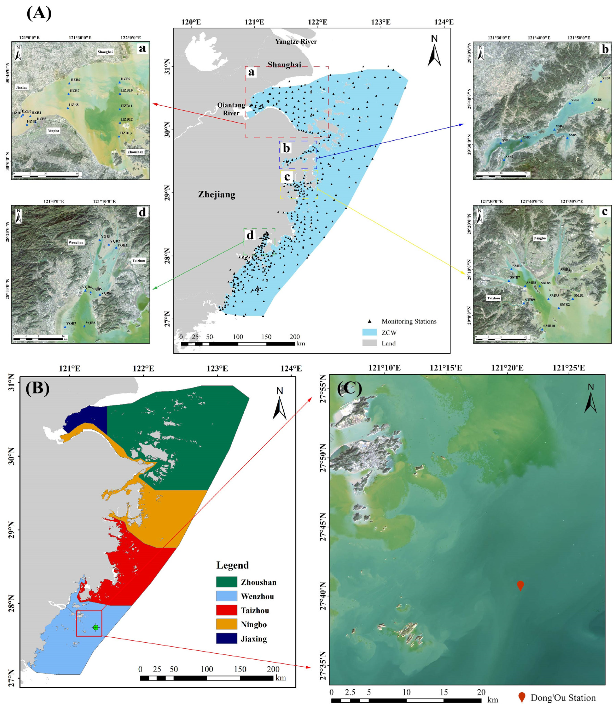
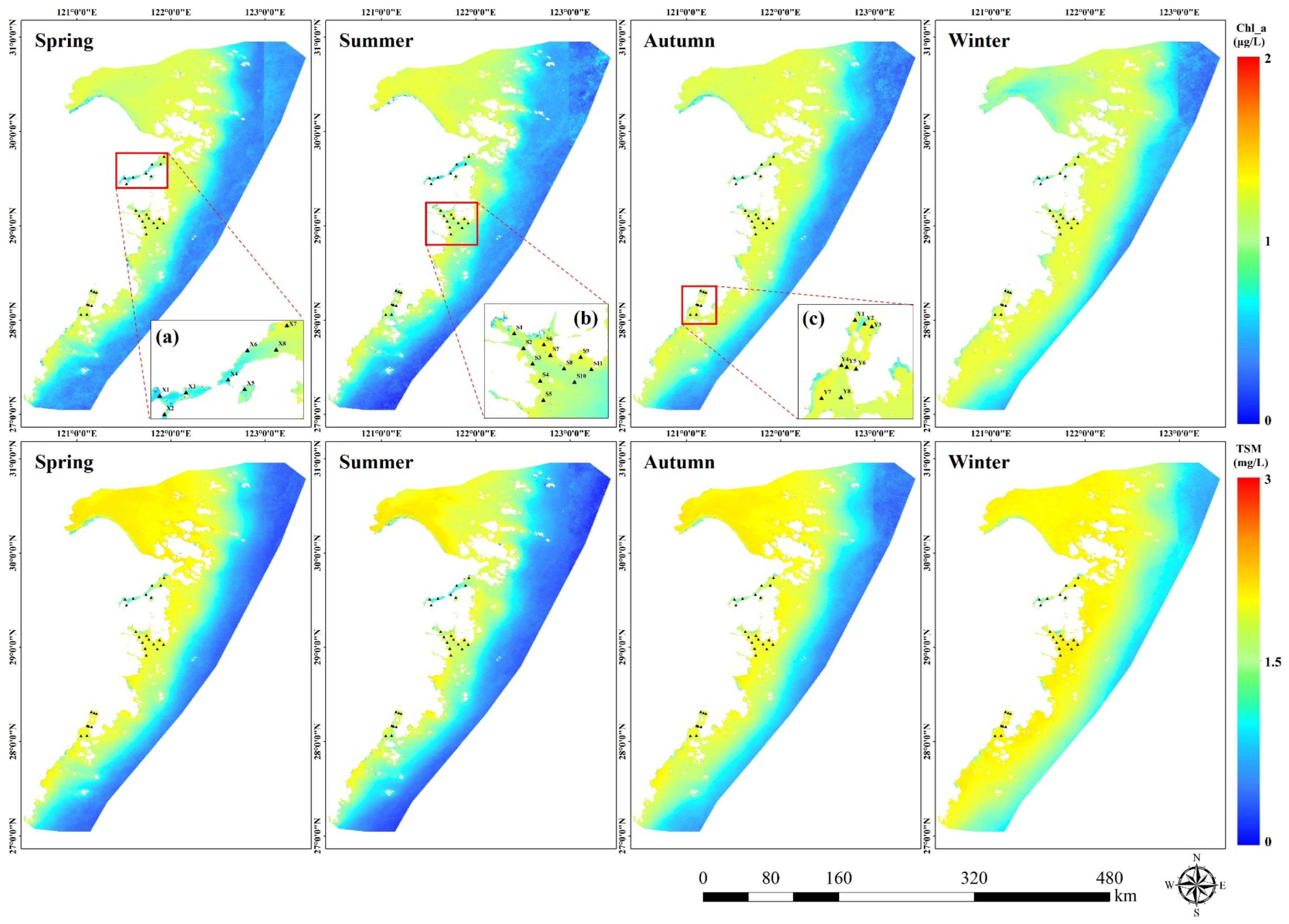
2.1. Study Area

Our study region is the ZCW, which includes four typical bays: the HZB, XSB, SMB, and YQB (a–d in Figure 1A). Located in the southeastern part of the East China Sea (27.0–31.0°N, 120.4–123.5°E), the jurisdictional sea area covers approximately 44,000 square kilometers, with a coastline extending over 6400 km. Influenced by the subtropical monsoon climate, the region has favorable heat, temperature, and moisture conditions, with average annual temperatures ranging between 15.7 and 17.9 °C. The temperature difference between the hottest and coldest months is approximately 20 °C, with an annual average rainfall of approximately 1335 mm and an average annual sunshine duration of 1710–2100 h. The southern part of the sea receives more rainfall and has higher temperatures than the northern part [25]. The abundance of spatial, economic, and biological resources, combined with a diverse ecosystem, makes the Zhejiang coastal region a dense hub for economic activities, such as aquaculture, tourism, shipping, and other industrial activities.

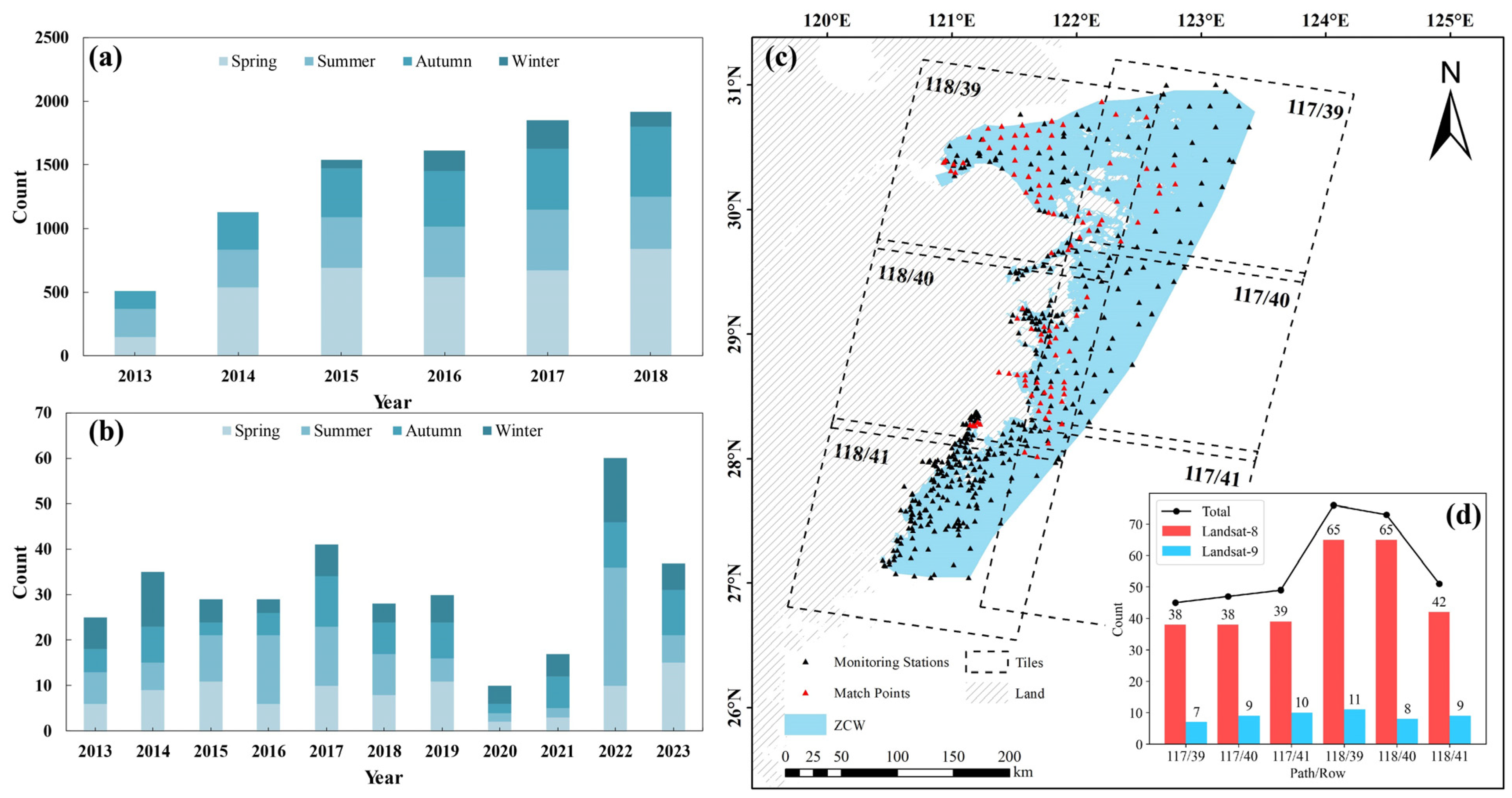
2.2. Satellite Data Acquisition and Processing

The primary sources of remote sensing data for this study were Landsat-8 and Landsat-9 images that covered the ZCW. These satellites were launched by the National Aeronautics and Space Administration (NASA) on 11 February 2013, and 27 September 2021, and were each equipped with operational land imagers (OLI and OLI-2) and thermal infrared sensors (TIRS and TIRS-2). While maintaining consistency in the number of bands, wavelength range, and spatial resolution, Landsat-9 is an improvement over Landsat-8 because of increased radiometric measurement precision, from 12-bit to 14-bit quantization, which enhances the overall signal-to-noise ratios and the performance of TIRS bands. Moreover, with an 8-day offset between the two satellites, their combined operation enables an increased observational frequency in the same area, effectively shortening the revisit interval. In this study, 341 Landsat images that cover the research area were downloaded from the United States Geological Survey Earth Explorer website (https://earthexplorer.usgs.gov/, as of 31 October 2023), including 287 images from Landsat-8 and 54 images from Landsat-9, and a statistical analysis of the temporal distribution of all the images was conducted (Figure 2b–d). Additionally, data on Chl-a and TSM concentrations were obtained from the Sentinel-3 OLCI imager’s Level-2 products, with a spatial resolution of 300 m and data available back to July 2017.

Atmospheric correction of the Landsat images involved the use of the dark spectrum fitting (DSF) algorithm developed by the Royal Belgian Institute of Natural Sciences (RBINS) and integrated into ACOLITE version 20231023.0 [26]. Previous research has demonstrated the efficacy of this method for Landsat images, particularly for processing turbid coastal waters and inland water bodies on a small scale. To ensure accuracy, this atmospheric correction method was validated using multispectral data recorded at the Dong’Ou monitoring station in the East China Sea (121.358356°E, 27.674966°N) [27] by the National Satellite Ocean Application Service. The correlation between the reflectance of Landsat’s visible bands after atmospheric correction and the measured reflectance, as well as comparisons of satellite reflectance and measured spectral reflectance across different seasons, with the matching data window controlled to within one hour, are illustrated (Figure 3). Overall, the satellite reflectance data obtained through this atmospheric correction method are consistent with the measured data, effectively capturing the reflectance of highly turbid waters in the ZCW. Based on this atmospheric correction approach, remote sensing reflectance (Rrs) data from the OLI/OLI-2 and SST data from the ST_B10 band of Landsat Level-2 products were used to establish the DO inversion model.

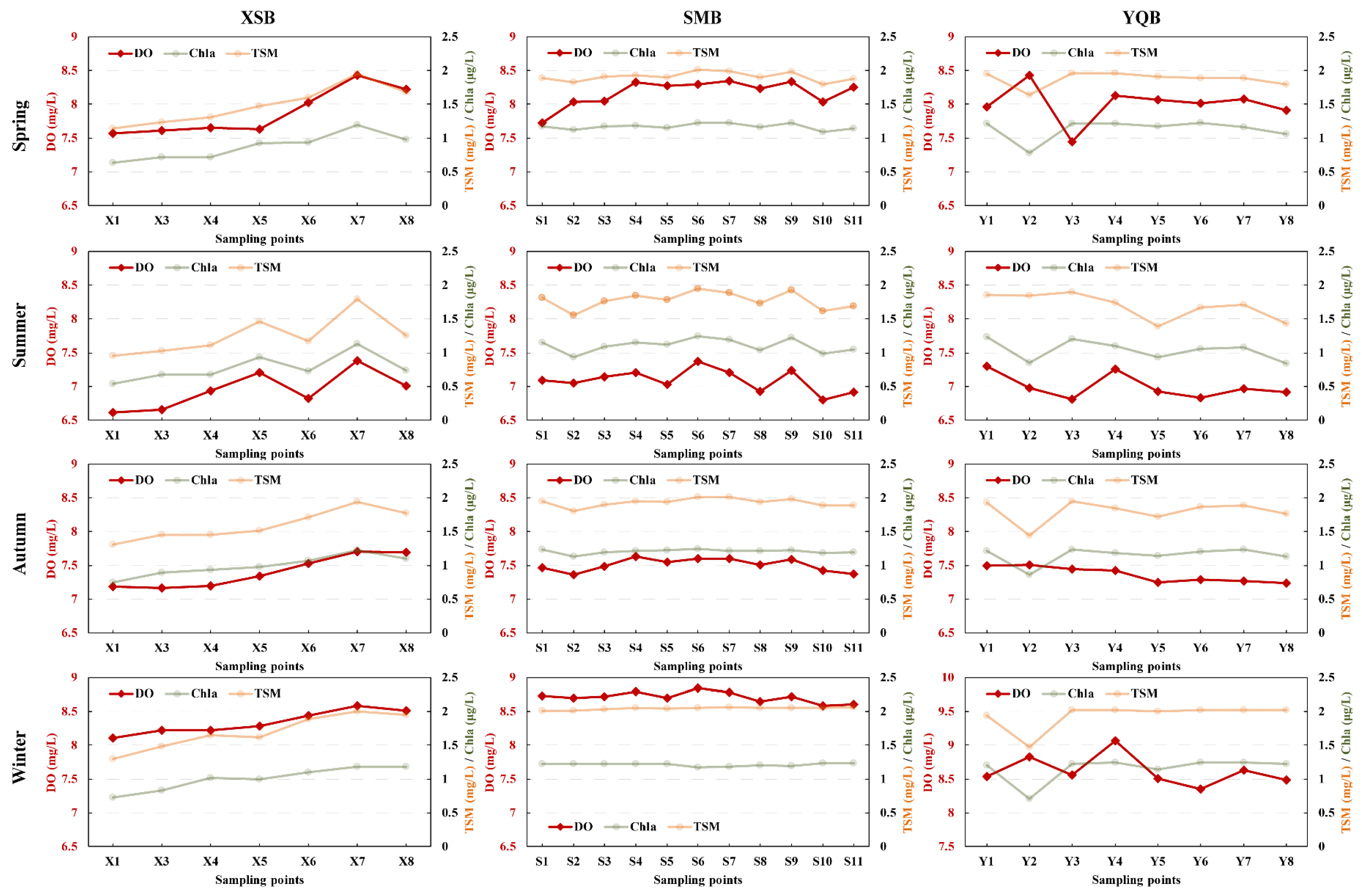
2.3. In Situ Measurement Data

The measurement data for this study were sourced from the Zhejiang Marine Monitoring and Forecasting Center and the Zhejiang Marine Ecology and Environment Monitoring Center, which offer water quality survey data for the ZCW from 2013 to 2018. The dataset includes data from more than 350 monitoring stations along the ZCW (Figure 1A), encompassing 8560 onsite observational records, with the majority of the data concentrated in spring, summer, and autumn (Figure 2a). Based on in situ data, spatial interpolation of the coastal DO concentration in Zhejiang yielded average DO concentrations for the spring, summer, and autumn seasons within the study area from 2013 to 2018 (Figure 4). Two primary factors are considered when matching the data from the field measurements with the data from the satellite observations: (I) the application of the coefficient of variation (CV) to eliminate spatial variability within the pixel corresponding to the field location and its surrounding 3 × 3 pixel area in the remote sensing images, thus minimizing the influence of mixed pixels, and (II) constraining the time interval between satellite passes and field observations within a certain range to accommodate rapid changes in the marine environment. The selection of CVs and time intervals aimed to balance the quality and quantity of matched data, which are important for the accuracy of the model. In this study, the time interval was limited to ±6 h, and Rrs data for any band pixel with a CV greater than 0.1 were excluded; only Rrs data with a CV less than 0.1 were matched [18,28]. Following these criteria, we ultimately obtained 95 pairs of matched data (Figure 2c).

2.4. Modeling Methods

As DO is a non-optically sensitive parameter, its relationship with satellite data is complex. Therefore, many studies use machine learning methods, such as support vector regression (SVR), artificial neural networks (ANN), and random forests (RF) to estimate DO levels [1,2,3,4]. However, based on prior explorations of the relationships between the Chl-a concentration, SST, and DO concentration, in this study, the aim was to develop an inversion model for DO concentrations along the ZCW. This model utilizes MLR, integrates Rrs and SST data, and includes a comprehensive evaluation of the assumptions underlying the regression analysis.

2.4.1. Multiple Linear Regression

MLR is a statistical model that is fitted based on a matched dataset and is capable of handling multiple independent variables to establish statistical relationships between several independent variables and a dependent variable. The MLR is particularly useful for analyzing the impact of multiple factors on the dependent variable, especially in cases of limited sample sizes [29]. The influence of different independent variables on the dependent variable can be represented through regression coefficients. The basic formula is given as follows:

$$y_i={\theta }_0+{\theta }_1{x}_1+{\theta }_2{x}_2+\dots +{\theta }_i{x}_i+{\epsilon }_i$$

(1)

where y_i represents the dependent variable; x₁, x₂, …, x_i represent the independent variables; θ₀, θ₁, θ₂, …, θ_i are the regression coefficients; and ε_i is the error term, which is assumed to follow a normal distribution [30]. When implementing the MLR algorithm, the least squares method is used to solve for the regression coefficients.

2.4.2. Model Performance Evaluation

The coefficient of determination (R²), adjusted R² (adj-R²), and root mean square error (RMSE) are important for assessing model performance. The R², which ranges from 0 to 1 and signifies the proportion of variance in the dependent variable that can be explained by the model, reflects its degree of fit. An R² value close to 1 indicates that the model has a strong predictive ability and can accurately fit the data. The specific method of calculation is illustrated in Equation (2):

$$R^2=1-\frac{S{S}_{res}}{S{S}_{tot}}=1-\frac{{\displaystyle {\sum }_{i=1}^n{({\widehat{y}}_i-y_i)}^2}}{{\displaystyle {\sum }_{i=1}^n{({\overline{y}}_i-y_i)}^2}}$$

(2)

$$R_{adj}^2=1-R^2\times (\frac{n-1}{n-k-1})$$

(3)

where SS_res represents the sum of squares of residuals, SS_tot represents the total sum of squares, y_i represents the observed values, ${\overline{y}}_i$ is the mean of the observed values, ŷ_i represents the predicted values, and n signifies the quantity of data. Within the realm of MLR, the increase in R² due to the addition of independent variables does not necessarily correlate with an improved fit, thereby necessitating the introduction of the adjusted R² (adj-R²) to assess the goodness of fit independently of the number of independent variables; this process mitigates the impact of the number of variables on R². The method for calculating the adj-R² is presented in Equation (3), where k denotes the number of independent variables in the model. The RMSE is a standard measure of the differences between actual observed values and those predicted by the model, and its method of calculation is detailed in Equation (4):

$$RMSE=\sqrt{\frac{{\displaystyle {\sum }_{i=1}^n{(y_i-{\widehat{y}}_i)}^2}}{n}}$$

(4)

2.4.3. MLR Hypothesis Testing

In MLR model analysis, the overall significance was verified with the F-test. If the F-statistic’s p-value was less than 0.05, the model was considered significant [31]. The significance of individual regression coefficients was assessed through the t-test, with a p-value less than 0.05 denoting that the respective coefficient is significant [32]. Variance inflation factors (VIF) help identify multicollinearity by measuring variance inflation. A VIF greater than 5 indicates potential multicollinearity issues, suggesting that the model may need further review or modification [33]. The normality of residuals was checked by analyzing standardized residuals with residual histograms and normal probability plots, ensuring that they followed a normal distribution [34]. These analyses were conducted using SPSS software version 27, employing the default parameters provided by the software for all the statistical analyses.

Based on the p value of the F-statistic, the specific method of calculation is given as follows:

$$F=\frac{{{\displaystyle {\sum }_{i=1}^n({\widehat{y}}_i-{\overline{y}}_i)}}^2/k}{S{S}_{res}/(n-k-1)}~F(k,n-k-1)$$

(5)

where SSR represents the sum of squares due to regression. The F-statistic follows an F-distribution with degrees of freedom (k, n – k − 1).

Based on the p-value of the t-statistic, the specific method of calculation is given as follows:

$$t=\frac{{\theta }_i}{S_{{\theta }_i}}~t(n-k-1)$$

(6)

where S_θi represents the standard error of the regression coefficient.

The VIF can be calculated using Equation (7) as follows:

$$VI{F}_i=\frac{1}{1-R_i^2}$$

(7)

3. Results

3.1. Model Construction and Validation

3.1.1. Model Construction

To accurately determine the changes in DO concentrations in the ZCW, we first aimed to construct and validate the model employed in this study. The data for developing the model were obtained by matching in situ measurements with satellite data and are summarized as follows: (I) 95 matched datasets; (II) DO concentrations ranging from 5.83 to 9.29 mg/L, averaging 7.74 mg/L; (III) 40 datasets for spring (March, April, and May), 19 datasets for summer (June, July, and August), 29 datasets for autumn (September, October, and November), and 7 datasets for winter (December, January, and February); and (IV) for the Rrs data, we acquired visible and near-infrared band data from Landsat-8/9, with central wavelengths ranging from 433 nm to 885 nm.

Based on the dataset, we expanded our analysis of Landsat-8/9 single-band images by combining the reflectance of six different bands to create 15 datasets with various band ratios. These ratios are used as inputs in our model, and they help reduce atmospheric effects and improve the precision of water quality parameters (WQPs) [35]. We performed a correlation analysis that connected six single bands, 15 band ratios, SST remote sensing data, and DO levels. The results showed a significant negative correlation of R = −0.74 between DO levels and SST values (Figure 5). Among the six single bands, Rrs_613, Rrs_655, and Rrs_865 had correlation coefficients (R) greater than 0.4, indicating moderate correlations. The rest of the bands show either weak (R < 0.4) or very weak (R < 0.2) correlations. Therefore, the SST and three single bands showing moderate correlations were used as inputs to the model. However, the size of the correlation coefficient should not be the only factor considered when choosing model inputs. Considering the benefits of band ratios, we also used band combinations with a correlation coefficient R > 0.1 as inputs. This approach led to the creation of MLR models that use single bands, band ratios, and SST to accurately estimate DO concentrations.

In our study, we divided the dataset into 80% for training (76 datasets across all seasons) and 20% for testing (19 datasets), ensuring seasonal representation in both datasets. Based on the strong correlation between SST and DO, SST was used as a fixed input variable for the model. Additionally, one and two remote sensing bands along with band ratio data were combined as independent variables to construct MLR models. The models were evaluated using R² and adj-R² values (

Table 1. Goodness of fit of MLR (R², coefficient of determination; adj-R², adjusted coefficient of determination; black bolded text indicates the best-fit MLR).

MLR Model	R2	adj-R2
Single Input
(1) DO = −1.154 × (Rrs_561/Rrs_613) − 0.069 × SST + 10.325	0.503	0.489
(2) DO = 30.469 × Rrs_613 − 0.07 × SST + 8.034	0.573	0.561
Multi-Input
(3) DO = 28.962 × Rrs_483 + 19.493 × Rrs_865 − 0.07 × SST + 8.193	0.592	0.575
(4) DO = 1.885 × (Rrs_561/Rrs_655) − 6.29 × (Rrs_483/Rrs_655) − 0.068 × SST + 14.932	0.554	0.536
(5) DO = 38.1165 × Rrs_655 + 0.88 × (Rrs_483/Rrs_613) − 0.069 × SST + 7.226	0.593	0.576

), showing the best-fit models under different independent variable inputs. The results indicated that the model had a significant response to the blue (Rrs_483) and red (Rrs_613, Rrs_655) bands of Landsat imagery, which are also commonly used to establish statistical relationships with the Chl-a and TSM concentrations [36,37,38]. Therefore, the model can explain the impact of SST on the DO concentration and reflects the relationships among the Chl-a, TSM, and DO concentrations to a certain extent, offering good interpretability and practical significance.

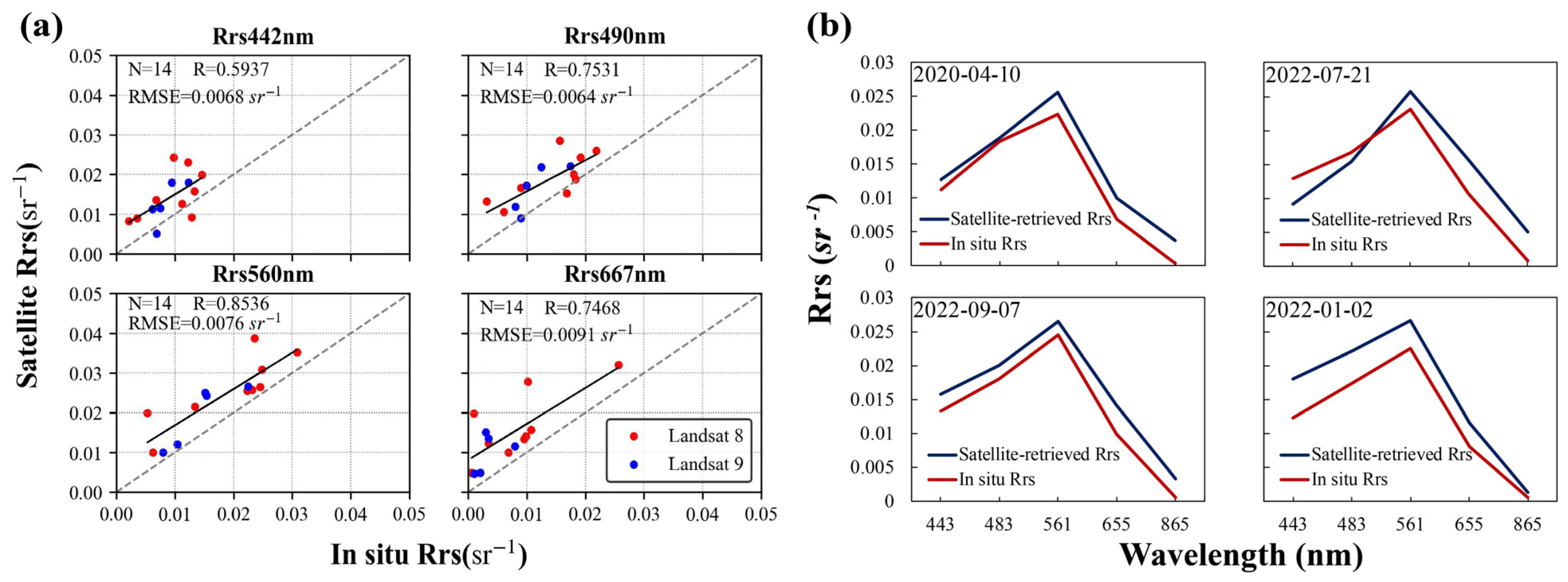
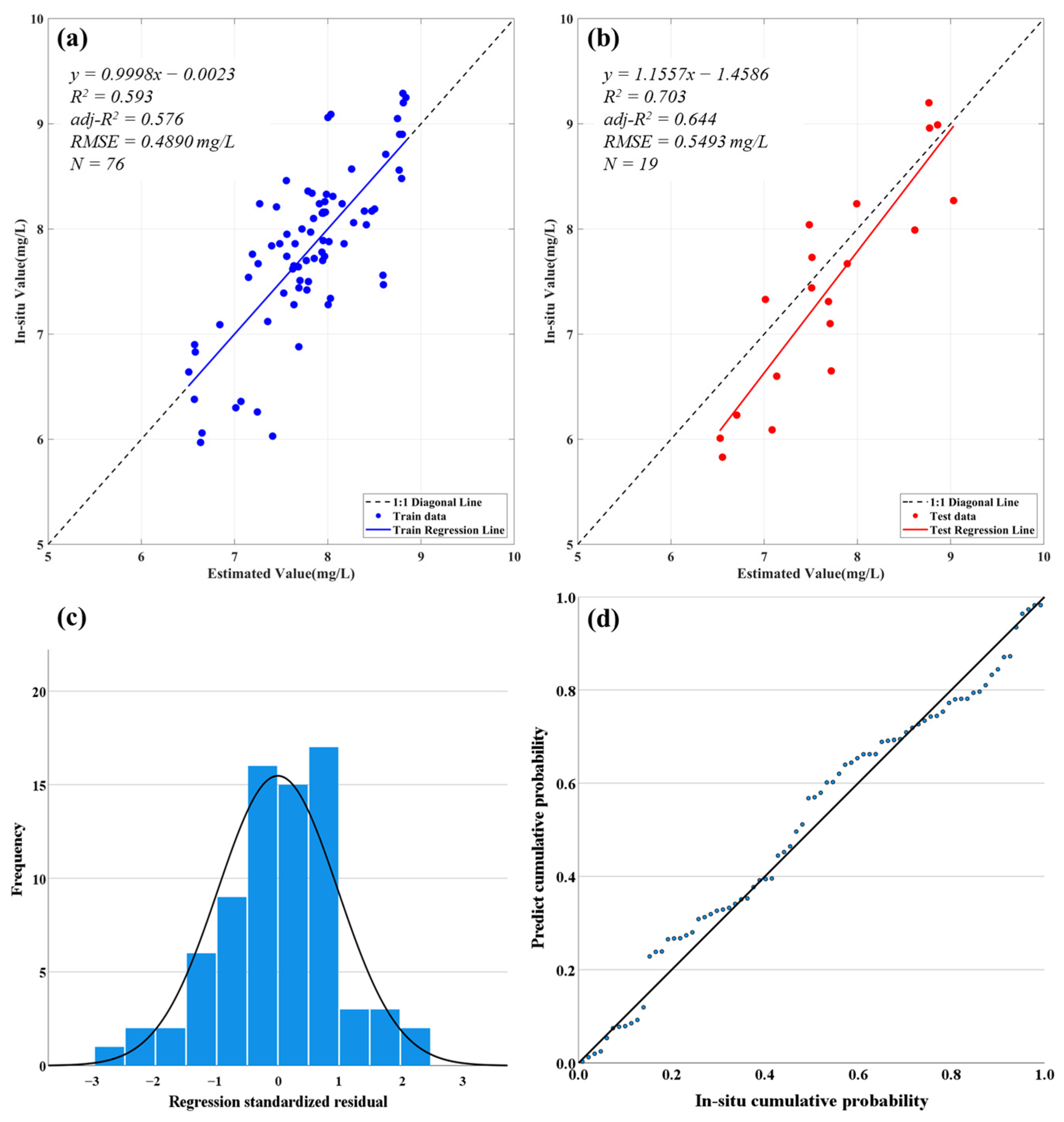
3.1.2. Model Validation

Based on the modeling results, we identified two models with the best training performance (Model-3 and Model-5), and the performance of these two models was assessed using the test dataset. The evaluation results indicate that Model-3 achieved an R² of 0.646, an adj-R² of 0.576, and an RMSE of 0.5999 mg/L for the test set, while Model-5 achieved an R² of 0.703, an adj-R² of 0.644, and an RMSE of 0.5493 mg/L for the test set (Figure 6a,b). Based on these results, Model-5 outperformed Model-3, leading to further hypothesis testing for Model-5.

We discovered a high correlation (R = −0.65) between Rrs_655 and the Rrs_483/Rrs_613 ratio in the set of independent variables for Model-5 (Figure 5), suggesting that the MLR model may have multicollinearity issues, which could lead to unstable model coefficients, thereby affecting the model’s accuracy and stability. To address this issue, metrics for assessing the significance and VIF were employed to test and evaluate the model’s significance and multicollinearity (

Table 2. Descriptive statistics of the coefficients of the best-fit model.

	Coefficient	Standard Error	t-Value	p-Value	VIF
Intercept	7.226	0.538	13.428	<0.001
Rrs_655	38.1165	7.321	5.206	<0.001	1.713
Rrs_483/Rrs_613	0.88	0.415	2.122	0.037	1.679
SST	−0.069	0.009	−7.584	<0.001	1.040

). (a) Regarding the regression equation, the F-test result was 34.95, with a p-value of less than 0.001, indicating that the regression equation passes the significance test. (b) In terms of regression coefficients, the t-test showed that the independent variables Rrs_655 and SST had considerable significance (p-value < 0.001), while the p-value for Rrs_483/Rrs_613 also reached the 0.05 level; hence, the regression coefficients also pass the significance test. (c) The VIF values for all three independent variables in the model were well below 5, indicating no multicollinearity issues or only weak collinearity. Additionally, the MLR model for inversely estimating DO concentrations included histograms and normal probability plots of residuals (Figure 6c,d), where the residuals essentially follow a normal distribution. In summary, Model-5 meets the assumptions of MLR and demonstrates good reliability when applied to the inverse estimation of DO concentrations.

Additionally, we compared the DO values inverted by the model with the in situ measurements observed on-site to verify the reliability of the satellite inversion results. The verification data were derived from monthly monitoring data at various monitoring sites in HZB, XSB, SMB, and YQB from 2015 to 2018 (Figure 1A). The inverted DO values for different seasons were compared with the results of in situ measurements (Figure 7). A comparison of the results indicates that the satellite inversion results were generally within the range of standard deviation of the corresponding in situ measurements. Only in certain seasons at individual sites in the HZB and XSB were the inverted values slightly underestimated, which may be due to the high turbidity of the water bodies in the region and the low effectiveness and temporal continuity of remote sensing data, which are particularly affected by frequent overcast and rainy weather in spring and summer, resulting in a greater number of missing values in the inversion results during these seasons. Therefore, after calculating the multiyear seasonal averages, there are certain differences between the calculated values and the measured results. Conversely, during the autumn and winter seasons, such differences are smaller. However, for different monitoring sites, both the satellite inversion results and in situ measurement results displayed a uniform spatial distribution pattern, without any significant fluctuations.

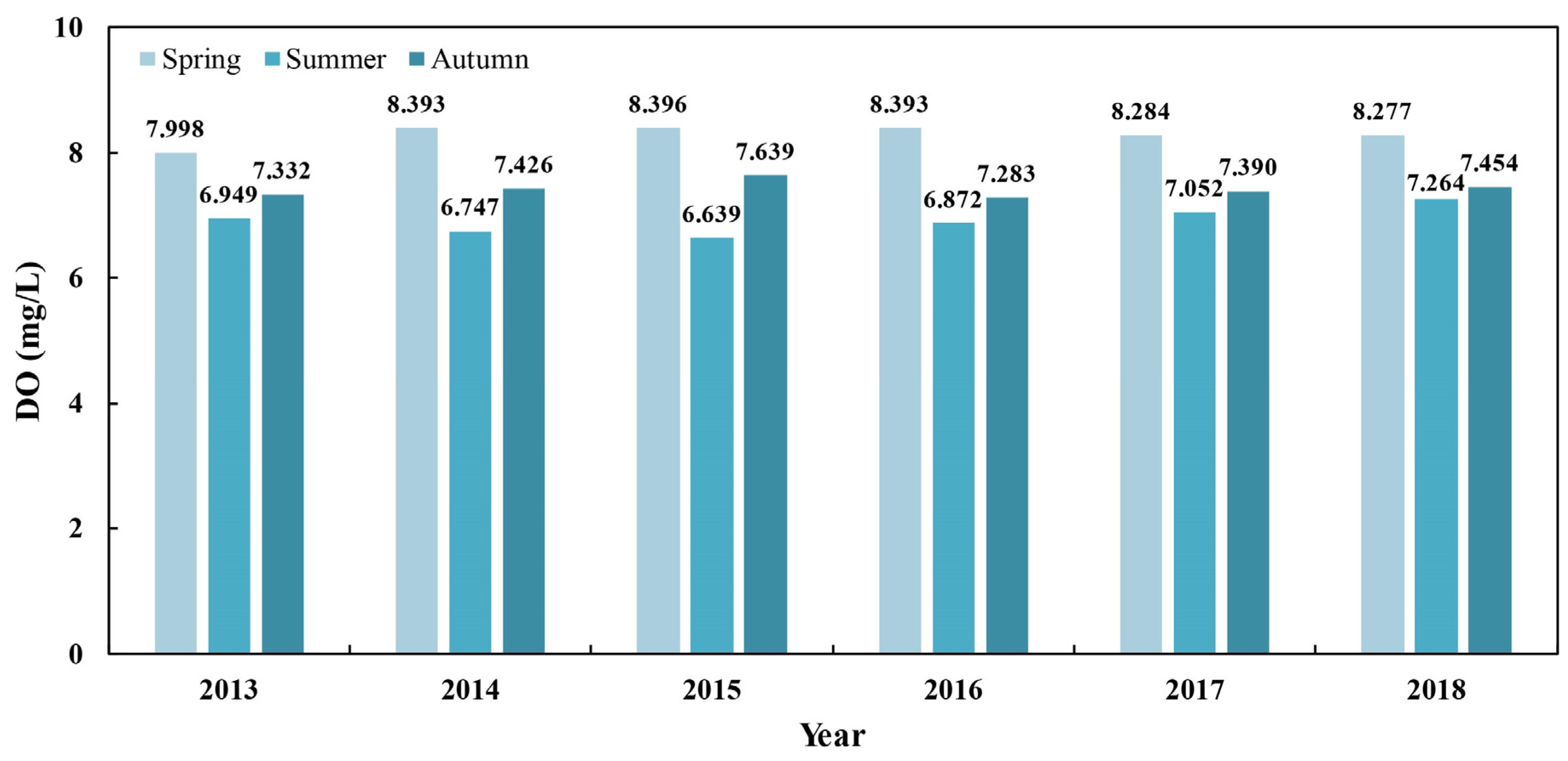
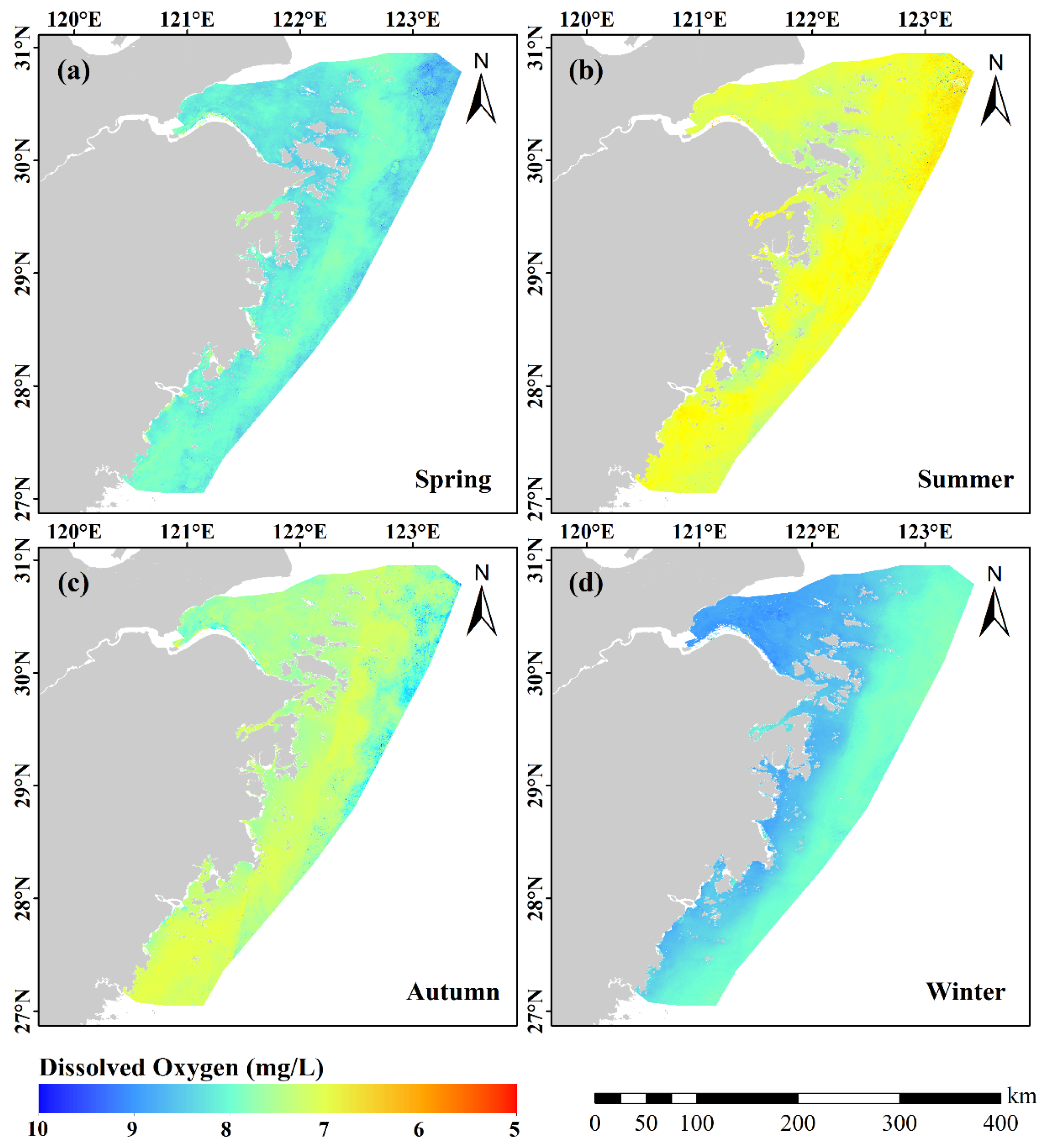
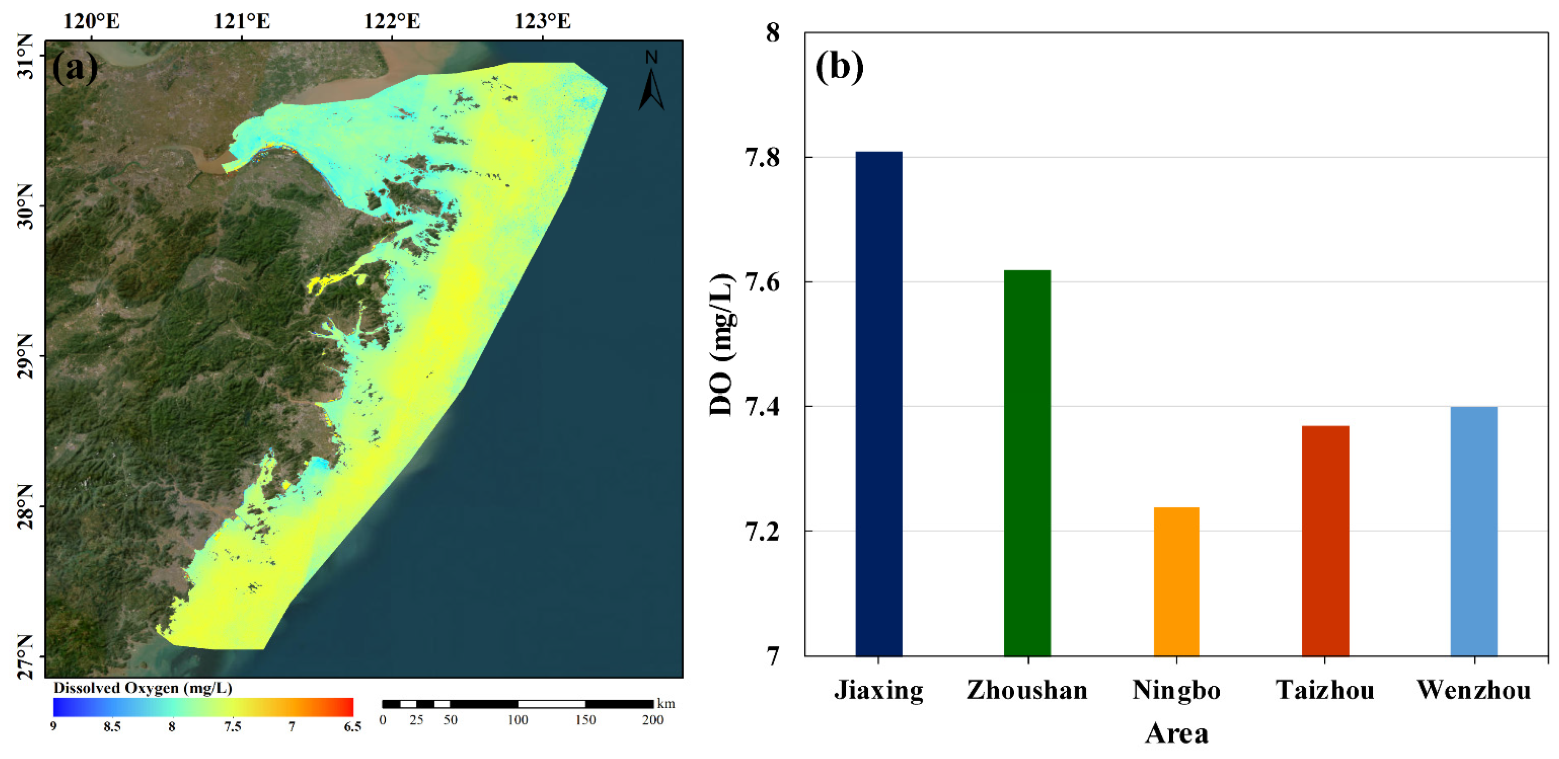
3.2. Temporal and Spatial Characteristics of DO

In this section, we analyzed the spatiotemporal variations in DO concentrations, aiming to determine their spatial distribution characteristics and seasonal distribution patterns. Based on the developed DO inversion model and Landsat data from 2013 to 2023, the multiyear average results for different seasons in the ZCW were inverted (Figure 8a–d). The inversion results revealed significant seasonal variations in the DO concentration in the ZCW, with higher concentrations in winter and spring than in summer and autumn. The highest and lowest values occurred in winter and summer, respectively. This conclusion was also supported by comparative validation results in the four typical bays, and the highest and lowest values of satellite inversion and in situ measurements, along with their corresponding locations, are shown (

Table 3. Maximum and minimum DO concentrations (mg/L) obtained from satellite inversion and on-site measurements in four typical bays and their monitoring stations.

Area	Satellite-Derived Value				In Situ Value
	Max		Min		Max		Min
	Station	DO	Station	DO	Station	DO	Station	DO
HZB	HZB2	9.02	HZB5	6.83	HZB4	9.51	HZB4	7.69
XSB	XSB7	8.59	XSB1	6.62	XSB5	9.27	XSB2	6.60
SMB	SMB3	8.77	SMB9	6.84	SMB6	9.18	SMB7	7.04
YQB	YQB4	9.06	YQB3	6.81	YQB8	8.85	YQB3	6.60

). Specifically, for HZB, the highest and lowest satellite-inverted values were 9.02 mg/L and 6.83 mg/L, respectively, while the highest and lowest measured values were 9.51 mg/L and 7.69 mg/L, respectively. For XSB, the highest and lowest satellite-inverted values were 8.59 mg/L and 6.62 mg/L, respectively, with measured values of 9.27 mg/L and 6.60 mg/L, respectively. For SMB, the satellite inversion yielded the highest and lowest values of 8.77 mg/L and 6.84 mg/L, respectively, compared to the measured values of 9.18 mg/L and 7.04 mg/L, respectively. Finally, for YQB, the highest and lowest satellite-inverted values were 9.06 mg/L and 6.81 mg/L, respectively, with the highest and lowest values of 8.85 mg/L and 6.60 mg/L, respectively.

From a seasonal spatial distribution perspective, the surface DO concentration exhibits distinct distributions in different seasons. In spring, the DO concentrations within the HZB exceeded those outside the bay, with lower concentrations noted around the Zhoushan Archipelago and its eastern waters, extending parallel to the coastline into the southern part of the ZCW. During summer, most sea areas had DO concentrations within the range of 6~8 mg/L, with a relatively uniform distribution. In autumn, overall, the DO concentrations within the entire sea area were higher near the coast and lower on the outer continental shelf, with high-value areas near the Yangtze River estuary in the northeast corner of the sea area and in HZB, where DO values were generally greater than 7.5 mg/L. High concentrations were also observed near the Zhoushan Archipelago east of 30°N. In winter, DO concentrations were generally greater near the coast than in the outer continental shelf areas, with low-concentration areas not exceeding 8 mg/L distributed parallel to the coastline from north to south. The areas west of the low-value zones closer to the shore generally showed DO values greater than 8.5 mg/L. This result was likely due to lower water temperatures, lower salinities, and higher gas solubilities in coastal waters compared to the slower temperature decreases, higher salinities, and lower gas solubilities in the outer continental shelf areas further from the coast. The analysis of the spatiotemporal distribution of surface dissolved oxygen near HZB from 2006 to 2007 by Li et al. [39] is generally consistent with the satellite inversion results of this study, indicating the highest DO concentrations in winter and the lowest in summer, with higher DO concentrations in the HZB area. Except for the relatively uniform distribution of DO concentrations in summer, the concentrations in the coastal areas were greater than those in the outer continental shelf areas. The findings of Shi et al. [40] indicate that during spring, DO concentrations in the ZCW were greater near the coast than offshore, with the highest values occurring near HZB, which agrees with the satellite inversion results of this study.

Based on the analysis at the seasonal scale, we further averaged the inverted DO concentrations from 2013 to 2023 to illustrate the spatial distribution of DO concentrations along the ZCW (Figure 9a). According to the figure, the DO concentrations in nearshore areas were evidently greater than those in the outer continental shelf areas. The DO concentrations in XSB and YQB were lower than those in HZB and SMB. Additionally, we calculated the multiyear average DO concentrations within the jurisdictional sea areas of five coastal cities (Figure 9b). The highest DO concentrations appeared on the shoreward side of HZB, with DO concentrations in southern ZCW being lower than those in the northern regions.

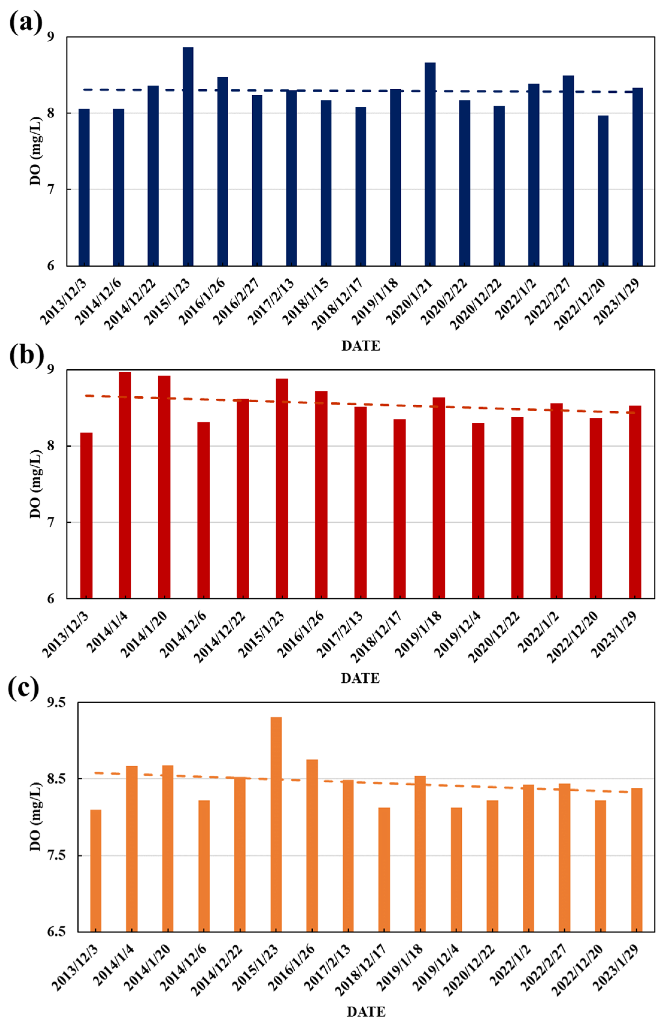
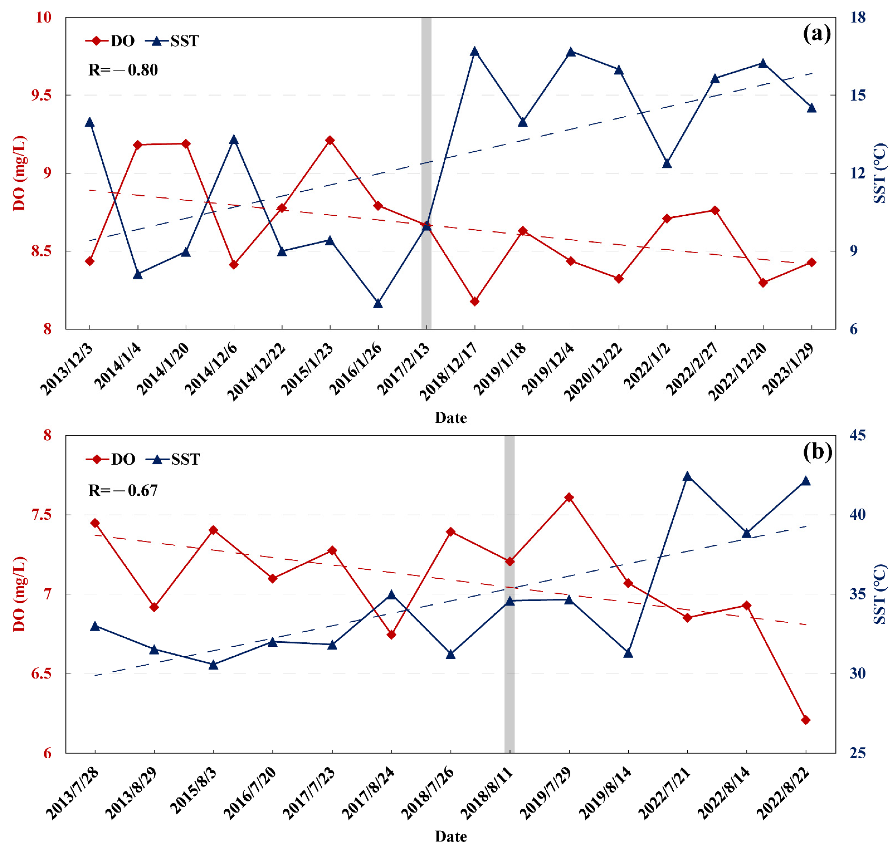
3.3. Long-Time Series Analysis

In this section, we analyzed the long-term variation in the DO concentrations to observe its long-term trends. We selected the remote sensing inversion results for the winter in XSB, SMB, and YQB. The inversion results for different years showed the following (Figure 10). Generally, the DO concentrations in January were slightly greater than those in December. From 2013 to 2023, in the winter seasons, the DO concentrations in the XSB fluctuated between 8 mg/L and 9 mg/L, with peaks occurring in January 2015 and January 2020; similarly, in SMB, the DO concentrations also fluctuated within the same range, with peaks occurring in 2014 and 2015. The pattern of fluctuation in the YQB was similar to that in the SMB, but the peak occurred in 2015 and exceeded 9 mg/L. Additionally, to more intuitively represent the changing trend in the DO concentration in the three areas from 2013 to 2023, a statistical regression analysis was performed on the time-series data (

Table 4. Results of the statistical regression analysis of changes in the DO concentrations.

Area	Time Interval	Slope	Intercept	R2
XSB	2013–2023	−0.002	8.315	0.0018
	2013–2023 (December)	−0.0166	8.1617	0.0546
	2013–2023 (January)	−0.046	8.6431	0.1810
SMB	2013–2023	−0.0157	8.6769	0.0845
	2013–2023 (December)	0.0148	8.3012	0.0566
	2013–2023 (January)	−0.0811	9.0708	0.966
YQB	2013–2023	−0.0168	8.5958	0.0658
	2013–2023 (December)	0.0062	8.2142	0.0057
	2013–2023 (January)	−0.0765	8.9879	0.2823

). A slope of less than 0 indicates a declining trend, with the magnitude of change being more significant if the absolute value of the slope is larger. This finding indicates significant changes in January for two areas, with the most significant changes occurring in SMB, followed by YQB. Overall, over the decade, the DO concentrations in the three areas slightly decreased and fluctuated, which is a phenomenon that warrants continuous monitoring.

4. Discussion

4.1. Effect of Chl-a and TSM Concentrations on DO

The study by Chen et al. [41] demonstrated direct or indirect correlations between Chl-a and TSM concentrations with DO, where their spatiotemporal variations also affect the spatiotemporal changes in DO. Therefore, in this section, taking XSB, SMB, and YQB as examples, based on the daily Chl-a and TSM products within the maritime areas governed by Zhejiang Province from Sentinel-3 data, we estimated the seasonal average Chl-a and TSM concentrations in XSB, SMB, and YQB from July 2017 to October 2023 (Figure 11). Then, we extracted Chl-a, TSM, and DO concentrations at different sampling points, further analyzing the impact of Chl-a and TSM concentrations on DO in different bays. The specific distribution of the sampling points is shown in Figure 11a–c.

We plotted the curves for Chl-a, TSM, and DO at different sampling points across three bays (Figure 12) and calculated the correlation coefficients between DO and Chl-a and TSM across different seasons (

Table 5. Correlation coefficients between DO and Chl-a concentrations and between DO and TSM concentrations across different seasons in each bay.

		Spring	Summer	Autumn	Winter
XSB	Chl-a	0.89	0.93	0.90	0.93
	TSM	0.95	0.96	0.95	0.97
SMB	Chl-a	0.43	0.81	0.73	−0.64
	TSM	0.59	0.81	0.86	0.01
YQB	Chl-a	−0.61	0.33	−0.32	−0.31
	TSM	−0.62	0.28	−0.14	−0.34

). The results indicate a highly significant positive correlation between DO and both Chl-a and TSM in the XSB waters, which may be related to the geographical characteristics of the bay. As a long and semi-enclosed bay with no large rivers flowing into it, water exchange is weak in the middle and upper parts of the bay, leading to a relatively stable aquatic environment. However, near the mouth of the bay, water exchange is strong and influenced by the Qiantang River and ocean currents, resulting in higher TSM concentrations and greater diversity and abundance of plankton [42]. Thus, higher concentrations of Chl-a occur here than in the middle and upper parts of the bay. The photosynthesis of Chl-a produces oxygen, thereby increasing the DO concentration at the surface; hence, the variation in the DO concentration in XSB is consistent with the changes in the Chl-a and TSM concentrations. In contrast, SMB, which has more rivers and estuaries and a more open bay, has stronger water exchange capabilities. The aquatic environment is significantly influenced by factors such as the Taiwan Warm Current, the Zhejiang-Fujian Coastal Current, and tides. Additionally, human activities are extremely prominent, with a high density of aquaculture areas and severe eutrophication conditions, leading to disparate correlations among Chl-a, TSM, and DO across different seasons. Even with higher correlation coefficients in summer and autumn, there is not necessarily consistency in the variations among TSM, Chl-a, and DO concentrations in SMB. Similarly, we found no explanatory correlation between Chl-a, TSM, and DO in YQB, even though the shape of YQB was similar to that of XSB. However, with approximately 30 rivers of various sizes flowing into it and a complex hydrodynamic environment [15], as well as shipyards, chemical plants, and thermal power plants scattered around the nearshore area of the YQB, the strong human impact and highly dynamic hydrological conditions mean that the DO in this area is not simply influenced by Chl-a and TSM. The specific underlying mechanisms still need to be explored in greater depth.

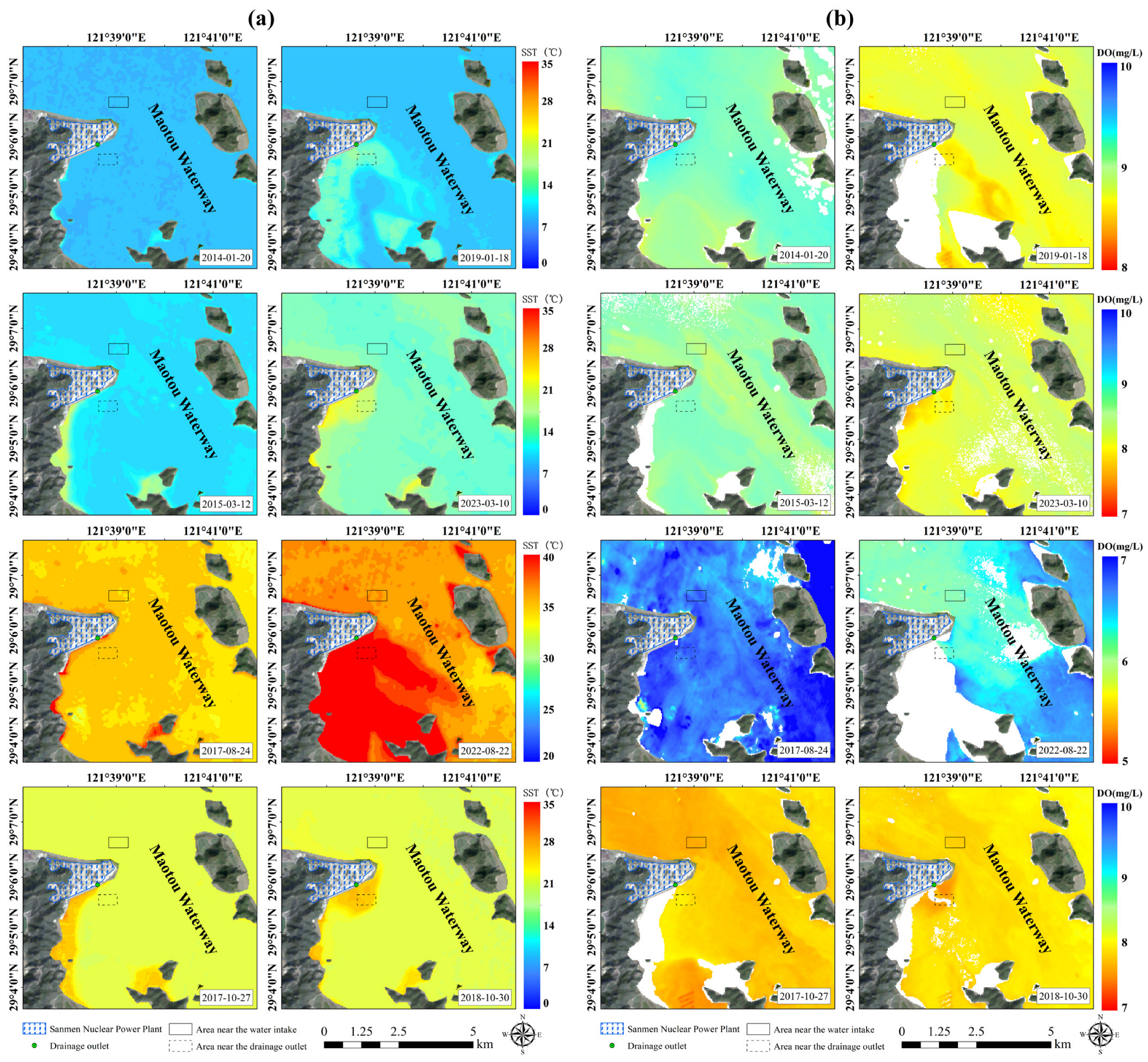
4.2. The Impact of Nuclear Power Plant Commissioning on DO

In this section, we use the SNPP as a case study to discuss the changes in DO concentrations within the range of impact of thermal discharge before and after its formal operation, and the thermal discharge data are derived from the Landsat level-2 SST product. Located in Sanmen County, Taizhou city, Zhejiang Province, and facing SMB, the first phase of the plant, consisting of two 1250 MW units, was connected to the grid in 2018. The water used for cooling comes from the Maotou waterway to the northeast, with the drainage outlet arranged on the beach outside the southern dike of the plant site [43] (Figure 13). Accordingly, we compared the changes in nearby SST (Figure 13a) and DO concentrations (Figure 13b) before (2013–2018) and after (2019–2023) the operation of the SNPP, with each row representing satellite inversion results for different months and depicting seasonal variations. The results indicate that before the operation of the SNPP, there was no significant difference between the SST near the discharge outlet and that near the intake, with a uniform distribution. However, after the commencement of plant operations, the SST near the drainage outlet was significantly greater than that near the intake, with the SST decreasing further from the drainage location. Before the operation of the nuclear power plant, no obvious low-DO areas were found near the drainage outlet; however, after the plant began operating, the DO concentration near the drainage outlet was notably lower than that in the surrounding waters, and the characteristics of the spatial distribution of the low-value area were similar to those of the thermal discharge. Wang et al., in their study on the impact of thermal discharge from the Daya Bay Nuclear Power Plant on the local marine ecosystem, also arrived at conclusions consistent with those in this study [44].

Additionally, we conducted a long-term analysis of the variations in the SST and DO concentrations in the sea area near the drainage outlet. To ensure a uniform temporal distribution of the data, we selected the remote sensing inversion results from winter (mainly in December and January) and summer (mainly in July and August) for analysis. In winter, before the operation of the SNPP, the SST fluctuated between 6 and 15 °C, and the DO concentrations ranged from 8.4 to 9.2 mg/L (Figure 14). After the SNPP began operation, the SST fluctuated between 12 and 17 °C, and the DO concentrations ranged from 8 to 8.8 mg/L, with a correlation coefficient of −0.80 between the SST and DO near the drainage outlet. In summer, before the operation of the SNPP, the SST fluctuated between 30 and 35 °C, and the DO concentrations ranged from 6.5 to 7.5 mg/L. After the SNPP began operation, the SST fluctuated between 30 and 42.5 °C, and the DO concentrations ranged from 6 to 7.6 mg/L, with a correlation coefficient of −0.67 between the SST and DO near the drainage outlet. Furthermore, by averaging the SST and DO over several years before and after the SNPP began operation, the results showed that the SST in winter increased by approximately 5.3 °C, which was an increase of approximately 53.05%, and the DO concentration decreased by approximately 0.36 mg/L, which was a decrease of approximately 4.1%. In summer, the SST increased by approximately 5.4 °C, which was an increase of approximately 16.66%, and the DO concentration decreased by approximately 0.25 mg/L, which was a decrease of approximately 3.5%. This finding demonstrated a significant negative correlation between the SST and DO near the drainage outlet of the SNPP. In both summer and winter, the operation of the SNPP and the resulting thermal discharge caused increasing SST near the drainage outlet, simultaneously leading to decreasing DO concentrations within a certain area.

4.3. Comparison with Previous Studies

In this section, we compare the methods and results of this study with those of previous similar research and discuss the innovations of the study, limitations of the model, and future outlook. Earlier literature reviews revealed that existing studies applied remote sensing techniques to the estimation of DO in coastal areas. For instance, KIM et al. utilized MODIS and VIIRS SST and Chl-a data to establish a multiple regression model that indirectly inferred temporal and spatial variations in dissolved oxygen along the western coast of South Korea. Their model achieved an R² of 0.801, indicating that marine reclamation was the main cause of the decrease in DO [22]. Arief et al. employed Landsat satellite SST data to indirectly infer DO concentrations along the Ringgung coast in Indonesia, achieving an R² of 0.562. They derived seasonal patterns of DO concentrations based on this model [23]. Summarizing previous research, we found a tendency to use optically sensitive factors that are highly correlated with DO, such as chlorophyll-a and SST, as model inputs. In contrast, our study not only utilized SST data that were significantly correlated with DO but also applied remote sensing reflectance data to the model. The final MLR model incorporated both the remote sensing band reflectance and SST as independent variables, achieving an R² of 0.644. The advantages of our model include the following: (1) error sources and uncertainties associated with indirect inference processes were reduced, making the results more direct and reliable; (2) strong real-time capabilities were provided by directly using remote sensing reflectance data, enabling a high temporal resolution suitable for dynamic monitoring and applications; and (3) more importantly, in the model results, we found that red and blue bands were more suitable for establishing a DO inversion model for ZCW, which also provides valuable references for future DO modeling for such complex water bodies. Additionally, for practical applications, we successfully inferred from our study the seasonal and spatial distribution patterns of DO in the entire jurisdictional waters of Zhejiang. Benefiting from the high resolution of Landsat imagery, we also conducted targeted monitoring and analysis of DO variations in typical bays and at the discharge outlets of nuclear power plants prone to hypoxia events, further enhancing the practical application of our study for water quality monitoring.

Nevertheless, our research still has the following limitations and areas for improvement: (1) In terms of the model, due to limitations in the amount of measured data, although the MLR model that we used is theoretically simple and intuitive and enhances model interpretability, its accuracy may decrease when handling nonlinear relationships. In recent years, the development of big data and artificial intelligence technologies has provided more efficient and accurate methods for establishing remote sensing inference models. Therefore, in the next step of our work, we plan to increase the scale of the measured data and select suitable machine learning algorithms to establish models with higher inference accuracy. Additionally, we aim to consider adding more factors related to DO to model inputs to facilitate analyzing the effects of each factor on DO changes, providing stronger technical support for coastal DO monitoring. (2) In terms of results analysis, we discussed the impact of water color factors on DO mainly because they affect light absorption and scattering, thereby influencing the efficiency of phytoplankton photosynthesis, ultimately affecting DO concentration. Therefore, in addition to Chl-a and TSM, CDOM, one of the three water color components, should also be included in the discussion. For instance, Jin et al. discussed the relationship between CDOM and coastal hypoxia dynamics in the Chesapeake Bay, finding significant differences in the impact of CDOM on nutrient dynamics and productivity between the upper bay, middle bay, and lower bay, emphasizing the necessity of comprehensively understanding the complex interactions between CDOM and hypoxia in coastal ecosystems [45]. However, due to the lack of reliable CDOM remote sensing products and field measurement data, we did not analyze the relationship between CDOM and DO. In future research, we plan to develop a CDOM remote sensing inversion model for the ZCW using reliable CDOM data and focus on analyzing the relationship between CDOM and DO inversion results.

5. Conclusions

In this study, using an MLR model combined with Landsat remote sensing data, a remote sensing model was successfully established for inverting DO concentrations in the ZCW, thereby enabling the temporal and spatial monitoring of DO concentrations in the ZCW from 2013 to 2023. The establishment and validation results of the model show that the red and blue bands are more suitable for building DO inversion models for complex water bodies. The model exhibited an R² of 0.593 and an adj-R² of 0.576, with an RMSE of 0.4890 mg/L for the training set; for the test set, the model achieved an R² of 0.703, an adj-R² of 0.644, and an RMSE of 0.5493 mg/L, effectively enabling DO concentration inversion. These results provide an accurate, cost-effective method for DO monitoring and offers a valuable reference for future DO modeling in similar complex water bodies. Furthermore, in this study, the impact of factors such as the Chl-a concentration, TSM concentration, and thermal discharge on the DO concentration were explored, revealing the potential impact of thermal discharge on the variations in DO concentrations in coastal waters.

The research results indicate significant seasonal variations in the DO concentration in the ZCW, with higher concentrations in winter and lower concentrations in summer. Additionally, DO concentrations in coastal areas were generally greater than those in outer continental shelf waters. The time series analysis revealed the most significant decreasing trend in the DO concentration in the SMB waters, followed by that in the YQB waters. This slight downward trend suggests the need for continuous monitoring of DO concentrations in these areas to identify and mitigate potential impacts on water quality deterioration in a timely manner. The Chl-a and TSM concentrations showed a significant positive correlation with the DO concentration in certain bay areas. However, this relationship is not universally applicable across all monitoring areas and is influenced by a variety of factors, including geographical location, hydrological conditions, and human activities. In particular, the operation of the SNPP has had a noticeable impact on the DO concentrations in the surrounding waters, with a significant negative correlation between the increase in seawater temperature caused by thermal discharge and the DO concentration, highlighting the potential impact of human industrial activities on the water quality of coastal waters.

This study provides an effective tool for monitoring and analyzing DO concentrations in the ZCW and has significant implications for understanding how thermal discharge influences marine water quality parameters and, consequently, coastal ecosystems. The results underscore the importance of continuous monitoring of water body DO concentrations to promptly detect and assess the impact of thermal discharge on marine environmental health and to provide a scientific basis for the protection and management of coastal waters. However, the current study has several limitations; firstly, a small amount of effective data was used for modeling, and the method and accuracy of the model need further improvement; secondly, regarding the three key factors of water color, due to the lack of reliable CDOM data, this study only discussed the impact of Chl-a and TSM on DO, without analyzing the effect of CDOM on DO. To address these shortcomings, future research should increase the scale of measured data, optimize modeling methods, and improve the accuracy of DO inversion, and explore the impact of CDOM on DO.

References

1. Mohseni, F.; Saba, F.; Mirmazloumi, S.M.; Amani, M.; Mokhtarzade, M.; Jamali, S.; Mahdavi, S. Ocean water quality monitoring using remote sensing techniques: A review. Mar. Environ. Res. 2022, 180, 105701. [Google Scholar] [CrossRef]
2. Coppola, L.; Legendre, L.; Lefevre, D.; Prieur, L.; Taillandier, V.; Riquier, E.D. Seasonal and inter-annual variations of dissolved oxygenin the northwestern Mediterranean Sea (DYFAMED site). Progress. Oceanogr. 2018, 162, 187–201. [Google Scholar] [CrossRef]
3. Dawson, J.; Orescanin, M.M.; Clark, R.; O’Connor, K. Spatiotemporal variability of dissolved oxygen in response to morphological state in a central California coast bar-built estuary. Estuar. Coast. Shelf Sci. 2023, 282, 108241. [Google Scholar] [CrossRef]
4. Abouelsaad, O.; Matta, E.; Omar, M.; Hinkelmann, R. Numerical simulation of Dissolved Oxygen as a water quality indicator in artificial lagoons–Case lagoons—Case study El Gouna, Egypt. Reg. Stud. Mar. Sci. 2022, 56, 102697. [Google Scholar] [CrossRef]
5. Zhang, X.; Wang, Z.; Cai, H.; Chai, X.; Tang, J.; Zhuo, L.; Jia, H. Summertime dissolved oxygen concentration and hypoxia in the Zhejiang coastal area. Front. Mar. Sci. 2022, 9, 1051549. [Google Scholar] [CrossRef]
6. Li, D.; Zhang, J.; Huang, D.; Wu, Y.; Liang, J. Oxygen depletion off the Changjiang (Yangtze River) estuary. Sci. China Ser. D Earth Sci. 2002, 45, 1137–1146. [Google Scholar] [CrossRef]
7. Wei, Q.; Wang, B.; Chen, J.; Xia, C.; Qu, D.; Xie, L. Recognition on the forming-vanishing process and underlying mechanisms of the hypoxia of the Yangtze River estuary. Sci. China Earth Sci. 2015, 58, 628–648. [Google Scholar] [CrossRef]
8. Wei, Q.; Wang, B.; Zhang, X.; Ran, X.; Fu, M.; Sun, X.; Yu, Z. Contribution of the offshore detached Changjiang (Yangtze River) Diluted Water to the formation of hypoxia in summer. Sci. Total Environ. 2021, 764, 142838. [Google Scholar] [CrossRef]
9. Guo, X.; Xu, B.; Burnett, W.C.; Wei, Q.; Nan, H.; Zhao, S.; Charette, M.A.; Lian, E.; Chen, G.; Yu, Z. Does submarine groundwater discharge contribute to summer hypoxia in the Changjiang (Yangtze) River Estuary? Sci. Total Environ. 2020, 719, 137450. [Google Scholar] [CrossRef]
10. Chen, X.; Shen, Z.; Li, Y.; Yang, Y. Physical controls of hypoxia in waters adjacent to the Yangtze Estuary: A numerical modeling study. Mar. Pollut. Bull. 2015, 97, 349–364. [Google Scholar] [CrossRef]
11. Chen, J.; Ni, X.; Mao, Z.; Wang, Y.; Liang, L.; Gong, F. Remote Sensing and Buoy Based Effect Analysis of Typhoon on Hypoxia off the Changjiang (Yangtze) Estuary. In Proceedings of the Remote Sensing of the Ocean, Sea Ice, Coastal Waters, and Large Water Regions 2012, Edinburgh, UK, 19 October 2012; pp. 257–264. [Google Scholar]
12. Qi, J.; Du, Z.; Wu, S.; Chen, Y.; Wang, Y. A spatiotemporally weighted intelligent method for exploring fine-scale distributions of surface dissolved silicate in coastal seas. Sci. Total Environ. 2023, 886, 163981. [Google Scholar] [CrossRef]
13. Andréfouët, S.; Costello, M.; Rast, M.; Sathyendranath, S. Earth observations for marine and coastal biodiversity and ecosystems. Remote Sens. Environ. 2008, 112, 3297–3299. [Google Scholar] [CrossRef]
14. Harvey, E.T.; Kratzer, S.; Philipson, P. Satellite-based water quality monitoring for improved spatial and temporal retrieval of chlorophyll-a in coastal waters. Remote Sens. Environ. 2015, 158, 417–430. [Google Scholar] [CrossRef]
15. Zhu, B.; Bai, Y.; Zhang, Z.; He, X.; Wang, Z.; Zhang, S.; Dai, Q. Satellite remote sensing of water quality variation in a semi-enclosed bay (Yueqing Bay) under strong anthropogenic impact. Remote Sens. 2022, 14, 550. [Google Scholar] [CrossRef]
16. Chen, J.; Ni, X.; Liu, M.; Chen, J.; Mao, Z.; Jin, H.; Pan, D. Monitoring the occurrence of seasonal low-oxygen events off the Changjiang Estuary through integration of remote sensing, buoy observations, and modeling. J. Geophys. Res. Ocean. 2014, 119, 5311–5322. [Google Scholar] [CrossRef]
17. Li, Y.; Robinson, S.V.J.; Nguyen, L.H.; Liu, J. Satellite prediction of coastal hypoxia in the northern Gulf of Mexico. Remote Sens. Environ. 2023, 284, 113346. [Google Scholar] [CrossRef]
18. Guo, H.; Huang, J.J.; Zhu, X.; Wang, B.; Tian, S.; Xu, W.; Mai, Y. A generalized machine learning approach for dissolved oxygen estimation at multiple spatiotemporal scales using remote sensing. Environ. Pollut. 2021, 288, 117734. [Google Scholar] [CrossRef]
19. Chatziantoniou, A.; Spondylidis, S.C.; Stavrakidis-Zachou, O.; Papandroulakis, N.; Topouzelis, K. Dissolved oxygen estimation in aquaculture sites using remote sensing and machine learning. Remote Sens. Appl. Soc. Environ. 2022, 28, 100865. [Google Scholar] [CrossRef]
20. Salas, E.A.L.; Kumaran, S.S.; Partee, E.B.; Willis, L.P.; Mitchell, K. Potential of mapping dissolved oxygen in the Little Miami River using Sentinel-2 images and machine learning algorithms. Remote Sens. Appl. Soc. Environ. 2022, 26, 100759. [Google Scholar] [CrossRef]
21. Zhang, Y.; Bai, Y.; He, X.; Li, T.; Jiang, Z.; Gong, F. Three stages in the variation of the depth of hypoxia in the California Current System 2003–2020 by satellite estimation. Sci. Total Environ. 2023, 874, 162398. [Google Scholar] [CrossRef]
22. Kim, Y.H.; Son, S.; Kim, H.C.; Kim, B.; Park, Y.G.; Nam, J.; Ryu, J. Application of satellite remote sensing in monitoring dissolved oxygen variabilities: A case study for coastal waters in Korea. Environ. Int. 2020, 134, 105301. [Google Scholar] [CrossRef]
23. Arief, M. Development of dissolved oxygen concentration extraction model using Landsat data case study: Ringgung coastal waters. Int. J. Remote Sens. Earth Sci. (IJReSES) 2015, 12, 1–12. [Google Scholar] [CrossRef]
24. Gholizadeh, M.H.; Melesse, A.M.; Reddi, L. A comprehensive review on water quality parameters estimation using remote sensing techniques. Sensors 2016, 16, 1298. [Google Scholar] [CrossRef]
25. Chen, Z.; Pan, D.; Bai, Y. Study of coastal water zone ecosystem health in Zhejiang Province based on remote sensing data and GIS. Acta Oceanol. Sin. 2010, 29, 27–34. [Google Scholar] [CrossRef]
26. Vanhellemont, Q.; Ruddick, K. Atmospheric correction of metre-scale optical satellite data for inland and coastal water applications. Remote Sens. Environ. 2018, 216, 586–597. [Google Scholar] [CrossRef]
27. Song, Q.; Chen, S.; Hu, L.; Wang, X.; Shi, X.; Li, X.; Deng, L.; Ma, C. Introducing Two Fixed Platforms in the Yellow Sea and East China Sea Supporting Long-Term Satellite Ocean Color Validation: Preliminary Data and Results. Remote Sens. 2022, 14, 2894. [Google Scholar] [CrossRef]
28. Cao, Z.; Ma, R.; Duan, H.; Pahlevan, N.; Melack, J.; Shen, M.; Xue, K. A machine learning approach to estimate chlorophyll-a from Landsat-8 measurements in inland lakes. Remote Sens. Environ. 2020, 248, 111974. [Google Scholar] [CrossRef]
29. Razi, M.A.; Athappilly, K. A comparative predictive analysis of neural networks (NNs), nonlinear regression and classification and regression tree (CART) models. Expert. Syst. Appl. 2005, 29, 65–74. [Google Scholar] [CrossRef]
30. Etemadi, S.; Khashei, M. Etemadi multiple linear regression. Measurement 2021, 186, 110080. [Google Scholar] [CrossRef]
31. Savin, N.E. Multiple hypothesis testing. Handb. Econom. 1984, 2, 827–879. [Google Scholar]
32. Loaiza, J.G.; Rangel-Peraza, J.G.; Monjardín-Armenta, S.A.; Bustos-Terrones, Y.A.; Bandala, E.R.; Sanhouse-García, A.J.; Rentería-Guevara, S.A. Surface Water Quality Assessment through Remote Sensing Based on the Box–Cox Transformation and Linear Regression. Water 2023, 15, 2606. [Google Scholar] [CrossRef]
33. Daoud, J.I. Multicollinearity and Regression Analysis. J. Phys. Conf. Ser. 2017, 949, 012009. [Google Scholar] [CrossRef]
34. Wiedermann, W.; von Eye, A. Direction of effects in multiple linear regression models. Multivar. Behav. Res. 2015, 50, 23–40. [Google Scholar] [CrossRef] [PubMed]
35. Adjovu, G.E.; Stephen, H.; James, D.; Ahmad, S. Measurement of Total Dissolved Solids and Total Suspended Solids in Water Systems: A Review of the Issues, Conventional, and Remote Sensing Techniques. Remote Sens. 2023, 15, 3534. [Google Scholar] [CrossRef]
36. Shi, K.; Li, Y.; Li, L.; Lu, H.; Song, K.; Liu, Z.; Xu, Y.; Li, Z. Remote chlorophyll-a estimates for inland waters based on a cluster-based classification. Sci. Total Environ. 2013, 444, 1–15. [Google Scholar] [CrossRef] [PubMed]
37. He, J.; Chen, Y.; Wu, J.; Stow, D.A.; Christakos, G. Space-time chlorophyll-a retrieval in optically complex waters that accounts for remote sensing and modeling uncertainties and improves remote estimation accuracy. Water Res. 2020, 171, 115403. [Google Scholar] [CrossRef] [PubMed]
38. Cai, L.; Tang, R.; Yan, X.; Zhou, Y.; Jiang, J.; Yu, M. The spatial-temporal consistency of chlorophyll-a and fishery resources in the water of the Zhoushan archipelago revealed by high resolution remote sensing. Front. Mar. Sci. 2022, 9, 1022375. [Google Scholar] [CrossRef]
39. Li, H.; Chen, J.; Lu, Y.; Jin, H.; Wang, K.; Zhang, H. Seasonal variation of DO and formation mechanism of bottom water hypoxia of Changjiang River Estuary. J. Mar. Sci. 2011, 29, 78–87. [Google Scholar]
40. Shi, X.; Wang, X.; Lu, R.; Sun, X. Distribution of dissolved oxygen and pH in frequent hab area of the East China Sea in spring 2002. Oceanol. Et Limnol. Sin. 2005, 36, 404. [Google Scholar]
41. Chen, J.; Pan, D.; Liu, M.; Mao, Z.; Zhu, Q.; Chen, N.; Zhang, X.; Tao, B. Relationships between long-term trend of satellite-derived chlorophyll-a and hypoxia off the Changjiang Estuary. Estuaries Coasts 2017, 40, 1055–1065. [Google Scholar] [CrossRef]
42. Xiuqing, H.; Ping, Q.; Weihua, Q. Research on the evaluation method of marine ecological environment in Xiangshan Bay. Acta Oceanol. Sin. 2015, 37, 63–75. [Google Scholar]
43. Qiang, Z.; Wei, C.; Jian, X.; Shao-qiao, L. Spatio-temporal characteristics of thermal discharge from Sanmen Nuclear Power Plant in winter based on field observations. Mar. Environ. Sci. 2022, 41, 847–856. [Google Scholar] [CrossRef]
44. Wang, Y.S.; Lou, Z.P.; Sun, C.C.; Sun, S. Ecological environment changes in Daya Bay, China, from 1982 to 2004. Mar. Pollut. Bull. 2008, 56, 1871–1879. [Google Scholar] [CrossRef] [PubMed]
45. Jin, R.; Gnanadesikan, A.; Pradal, M.-A.S.; St-Laurent, P.J.A.P. How does colored dissolved organic matter (CDOM) influence the distribution and intensity of hypoxia in coastal oceans? Authorea Prepr. 2023. [Google Scholar] [CrossRef]
Figure 1. (A) Schematic representation of the study area and positions of various monitoring sites. Points (ad) denote the locations and satellite imagery of the HZB, XSB, SMB, and YQB, respectively. The blue triangles represent the positions of the in situ sampling points used for verification. (B) Jurisdictional sea area boundaries of coastal cities in Zhejiang and the location of the Dong’Ou Monitoring Station. (C) Satellite image of the area surrounding the Dong’Ou Monitoring Station (the red mark indicates the position of the station).
Remotesensing 16 01951 g001
Figure 2. Temporal and spatial distributions and statistics of the research data: (a) temporal distribution of the field observation data, (b) seasonal distribution of the Landsat image data, (c) spatial distribution of the Landsat images and matched data points, and (d) volume of data for each Landsat image scene.
Remotesensing 16 01951 g002
Figure 3. (a) Correlation between the optical band reflectance of Landsat images corrected by Acolite atmospheric correction and measured data. In the figure, Rrs represents the remote sensing reflectance, and RMSE represents the root mean square error, the dashed line represents a 1:1 fitting line, while the solid line represents the degree of fit between the measured data and remote sensing data. (b) Comparisons between the satellite-retrieved and in situ Rrs.
Remotesensing 16 01951 g003
Figure 4. Temporal variation in average DO concentrations from field observations along the ZCW from 2013 to 2018.
Remotesensing 16 01951 g004
Figure 5. Correlations between DO and various elements.
Remotesensing 16 01951 g005
Figure 6. Model evaluation: (a) training results for Model-5. (b) Testing results for Model-5. (c) Histogram of standardized residuals. (d) Normal probability plot (probability p-p plot) for DO residuals.
Remotesensing 16 01951 g006
Figure 7. Comparison between satellite-derived and in situ DO values across different seasons in four typical bays (ad). The red line represents the seasonal average of in situ data, while the blue line denotes the seasonal average derived from satellite inversion.
Remotesensing 16 01951 g007
Figure 8. Seasonal spatial distribution of DO concentrations in the ZCW based on remote sensing inversion from 2013 to 2023. (a) Spring, (b) Summer, (c) Autumn, (d) Winter.
Remotesensing 16 01951 g008
Figure 9. (a) Spatial distribution of average DO values from 2013 to 2023; (b) average DO values in maritime areas governed by five coastal cities from 2013 to 2023.
Remotesensing 16 01951 g009
Figure 10. Long-term variations in the average DO concentrations in XSB, SMB, and YQB, the dashed line represents the long-term trend of change. (a) XSB; (b) SMB; (c) YQB.
Remotesensing 16 01951 g010
Figure 11. Average distributions of Chl-a and TSM concentrations in the ZCW from July 2017 to October 2023, the black triangle represents the location we are analyzing. (a) Distribution of sampling points in XSB; (b) distribution of sampling points in SMB; (c) distribution of sampling points in YQB.
Remotesensing 16 01951 g011
Figure 12. Relationships between the DO concentration and Chl-a and TSM concentrations at different sampling locations.
Remotesensing 16 01951 g012
Figure 13. (a) Comparison of SST changes near the SNPP before and after operation; (b) comparison of changes in the DO concentration near the SNPP before and after operation (the dashed boxes represent the water area near the drainage outlet, while the solid boxes represent the water area near the water intake).
Remotesensing 16 01951 g013
Figure 14. Temporal variation in the SST and DO near the drainage outlet of the SNPP before and after the operation began, the dashed line represents the trend line of change. (a) Winter. (b) Summer (to the left of the gray bar in the figure, the changes before the SNPP operation began are shown, while to the right of the gray bar, the changes after the SNPP operation began are shown).
Remotesensing 16 01951 g014