Deep Multi-Order Spatial–Spectral Residual Feature Extractor for Weak Information Mining in Remote Sensing Imagery

Abstract

Remote sensing images (RSIs) are widely used in various fields due to their versatility, accuracy, and capacity for earth observation. Direct application of RSIs to harvest optimal results is generally difficult, especially for weak information features in the images. Thus, extracting the weak information in RSIs is reasonable to promote further applications. However, the current techniques for weak information extraction mainly focus on spectral features in hyperspectral images (HSIs), and a universal weak information extraction technology for RSI is lacking. Therefore, this study focused on mining the weak information from RSIs and proposed the deep multi-order spatial–spectral residual feature extractor (DMSRE). The DMSRE considers the global information and three-dimensional cube structures by combining low-rank representation, high-order residual quantization, and multi-granularity spectral segmentation theories. This extractor obtains spatial–spectral features from two derived sequences (deep spatial–spectral residual feature (DMSR) and deep spatial–spectral coding feature (DMSC)), and three RSI datasets (i.e., Chikusei, ZY1-02D, and Pasture datasets) were employed to validate the DMSRE method. Comparative results of the weak information extraction-based classifications (including DMSR and DMSC) and the raw image-based classifications showed the following: (i) the DMSRs can improve the classification accuracy of individual classes in fine classification applications (e.g., Asphalt class in the Chikusei dataset, from 89.12% to 95.99%); (ii) the DMSC improved the overall accuracy in rough classification applications (from 92.07% to 92.78%); and (iii) the DMSC improved the overall accuracy in RGB classification applications (from 63.25% to 63.6%), whereas DMSR improved the classification accuracy of individual classes on the RGB image (e.g., Plantain classes in the Pasture dataset, from 32.49% to 39.86%). This study demonstrates the practicality and capability of the DMSRE method to promote target recognition on RSIs and presents an alternative technique for weak information mining on RSIs, indicating the potential to extend weak information-based applications of RSIs.

1. Introduction

Remote sensing images (RSIs) can capture details of ground objects [1]; thus, they are widely used in agriculture, military, resource exploration, and change detection [2,3,4,5]. Information extraction is one of the most important step in RSI processing and plays a significant role in the application of RSIs [6]; however, information extraction from RSIs still remains challenging [7], especially in weak information. Weak information features in RSIs generally refer to information that is less apparent or easily overshadowed by surrounding features [8], and weak information is hard extract after preprocessing [9], e.g., soil salinity [10], heavy metals [11]. Achieving optimal results for weak information features can be challenging. Therefore, developing an approach for efficient mining of weak information in RSIs is necessary to facilitate and promote their application.

The feature extraction (FE) technique is an effective way to address the challenging task of information extraction in RSIs [12]. This technique helps extract suitable feature information from the raw RSIs for remote sensing [13]. The most common FE techniques for RSIs can be divided into three major categories: spectral-, spatial-, and spatial–spectral-based FE methods. Classical spectral-based FE methods for RSIs, such as principal component analysis (PCA) [14] and linear discriminant analysis (LDA) [15], are widely applied. PCA identifies the projection with the minimum data reconstruction error, while LDA aims to retain the information necessary to separate the target classes [16]. However, the above methods are unsuitable for modeling the nonlinear relationships for complex RSI data [17,18]. Thus, numerous extension methods based on PCA and LDA, such as robust PCA [19], sparse PCA [20], subspace LDA [21], regularized LDA [22], and so on [23,24,25], have been proposed. Several other techniques have also been introduced to tackle this problem and achieve highly advantageous results, such as utilizing locality-preserving projection [26], locality-preserving nonnegative matrix factorization [27], nonnegative matrix factorization [28], and Gaussian mixture models [29]. However, the spectral-based FE methods are commonly known as the dimensionality reduction method, which loses the detailed information and the spectral relationship of RSIs.

In the context of spatial-based FE methods, the gray-level co-occurrence matrices, Gabor wavelets [30], morphological profiles (MPs) [31], and Markov random fields [32] are widely applied. However, the spatial-based FE methods via neighborhoods of pixels were limited by the scale selection and the detailed content of very high-resolution images [33]. Akcay et al. [33] exploited the structural information of RSIs using morphological operators to address these problems and achieved excellent performance. Mallinis et al. [34] extracted local patterns of images via texture measurement methods and yielded superior classification results. However, the use of only spatial or spectral information may occasionally be insufficient to achieve desired results [17]. Therefore, combining the spatial and spectral information of RSIs has the potential to achieve high performance in FE.

As imaging technology continues to evolve, the spatial resolution of RSIs has significantly increased. This advancement enhances the accuracy of RSI applications by incorporating spatial information of neighboring positions into spectral-based feature extraction methods [35]. Therefore, numerous spatial-based FE methods have been introduced into spectral-based FE methods to construct spatial–spectral-based FE methods. The extended MPs were developed for spatial–spectral feature extraction of RSIs [36] and obtained a better classification result. Kang et al. [37] extracted the spatial–spectral features via edge-preserving filtering, which assumed the correlation among neighboring objects, and significantly improved the classification accuracy. In addition, the deep learning (DL) method has achieved remarkable achievements in the spatial–spectral-based FE method in RSIs [38,39]. Chen et al. [40] introduced a deep belief network to the extract spatial–spectral features of RSIs and achieved a high accuracy of classification results. Based on deep belief network, Ma et al. [41] added a regularization term to extract spectral–spatial features by introducing an energy function in a spatially updated deep auto-encoder, thereby providing encouraging results. Moreover, Kavitha et al. [42] proposed that a deep e-CNN model using a spatial–spectral feature merging strategy effectively improves the classification performance. However, the spatial–spectral-based FE method based on DL needs a large number of training samples, which increases its nonuniversality.

In the context of weak information extraction methods for RSIs, Kang [43,44] introduced a multi-granularity spectral segmentation (MGSS) technique addressing hyperspectral weak information mining and achieved excellent performance in the quantitative application of remote sensing. MGSS enables multi-granularity segmentation (MGS) and multi-granularity reconstruction (MGRS) of spectral data via multi-granularity residual (MGR). Kang [45] proposed an optimal pixel-based residual spectral reconstruction method based on the MGRS and improved estimation accuracy of aboveground biomass on grasslands. Building on the foundation of the MGR, Pang et al. [46] simulated hyperspectral data using the multispectral of sample points and achieved favorable results in grassland micronutrient estimation. Fan et al. [10] expanded the MGSS to soil salinity monitoring and found that MGSS technology can effectively extract weak spectral information from soil, compared with the traditional spectral preprocessing methods, significantly improved the correlation between spectra and soil. An increasing number of reports have addressed this technology since the introduction of MGSS. However, the MGSS method focuses on the spectral domain and disregards the spatial information of RSIs, which limits its application in remote sensing.

The current study attempts to develop a spatial–spectral-based FE technique to address the aforementioned problem. This technique can comprehensively consider the three-dimensional structure and global information of RSIs to mine the weak information in RSIs. Inspired by MGSS theory, this study proposes a novel spatial–spectral-based FE technique by combining low-rank presentation (LRR), high-order residual quantization (HORQ), and MGSS and discusses the characteristic and practicality of the extracted feature via its classification results.

2. Basic Methodology

HORQ, MGSS, and LRR are the important foundations of the proposed method. HORQ and MGSS are used to mine the weak information in theory, and LRR is used to explore the global structure of RSIs. Therefore, the four underlying components are briefly reviewed in this section.

2.1. High-Order Residual Quantization

The HORQ technique [47] was proposed to accelerate and compress neural networks. Building on the foundation of XNOR-Net [48], HORQ incorporates +1 or −1 Binary Coding (BC ± 1) [49] to achieve significant computational acceleration while maintaining network accuracy. HORQ approximates the high-dimensional vector $X$ as $\mathrm{X}\approx {\mathsf{\beta }}_1{\mathrm{H}}_1$, where $H_1$ represents the BC ± 1 coding matrix of $X$, and ${\beta }_1$ is a positive factor, which denotes the weighting coefficient of ${ H}_1$. The estimations for $X$ and ${\beta }_1{H}_1$ are as follows:

$$\begin{array}{c}{\beta }_1^{*},H_1^{*}=\underset{{\beta }_1,H_1}{argmin}({\beta }_1,H_1)\\ =\underset{{\beta }_1,H_1}{argmin}{‖X-{\beta }_1{H}_1‖}_{l_2}\end{array}.$$

(1)

Considering Formula (1), Li [47] and Rastegari [48] provided comprehensive descriptions of its analytical steps. The solution was as follows:

$$\left\{\begin{array}{c}{\beta }_1^{*}=\frac{1}{N}{‖X‖}_{l_1}\\ H_1^{*}=sign\left(X\right)\end{array}\right.,$$

(2)

where $sign\left(X\right)$ represents the sign function of $X$. Furthermore, concerning the residual of $X$, Li defined residual as follows [47]:

$$R_{i-1}\left(X\right)=X-{\sum }_{i=1}^N{\beta }_i{H}_i,$$

(3)

where N is a positive integer greater than 1, and the encoding feature of $X$ at i-order is defined as follows:

$$C_i\left(X\right)={\beta }_i{H}_i.$$

(4)

2.2. Multi-Granularity Spectral Segmentation

Based on the HORQ method, Kang et al. [43] introduced high-order binary coding (HOBC) for hyperspectral images (HSIs), which enables high-performance coding compression and lossless recovery of HSIs. Subsequently, Kang [45] extended HOBC to introduce the MGSS technique. MGSS involves continuous quantization and decomposition of the spectral information and mines weak spectral features within specific wavelength ranges. This technique assumes the acquisition of spectral vectors as G, and its Nth order reconstructed features can be expressed as follows:

$$\begin{array}{cc}G& =\hspace{0.33em}{\sum }_{i\hspace{0.33em}=\hspace{0.33em}1}^N{\beta }_i{H}_i\hspace{0.33em}+\hspace{0.33em}{R}_N\left(G\right)\end{array}\approx \hspace{0.33em}{\sum }_{i\hspace{0.33em}=\hspace{0.33em}1}^N{\beta }_i{H}_i.$$

(5)

Kang [43] provided detailed derivations and explanations of the analytical derivation of Formula (6). Thus, ${\beta }_i$ and $H_i$ can be represented as below:

$$\left\{\begin{array}{cc}{\beta }_i& =\frac{1}{N}\Vert R_{i-1}\left(G\right){\Vert }_{l_1}\\ H_i& =sign\left(R_{i-1}\right(G\left)\right)\end{array}\right..$$

(6)

The MGSS technique performs spectral feature decomposition on sampled points to attain per-pixel spectral features of RSIs. However, the aforementioned methods concentrate on spectral features on a per-pixel basis, disregarding the three-dimensional structure that is inherent in RSIs.

2.3. Low-Rank Representation of RSIs

The RSI is a three-dimensional cube that combines imagery and spectral characteristics. LRR is the introduced technique to fully consider the global spatial and spectral information of raw images. LRR is widely used in image processing due to its impressive performance in capturing the global data structure [50]. Therefore, LRR is proposed for RSIs to mine their global spectral–spatial character. During the FE process, the three-dimensional RSI is transformed into a two-dimensional low-rank matrix to incorporate the global spatial–spectral information, allowing for globally optimized extracted features. Figure 1 shows the flowchart of the LRR for RSIs.

Suppose $G\in H^{m\times n\times b}$ is the achieved RSI, $m\times n$ is the spatial size of $G$, and $b$ is its band number. Thus, $G$ can be introduced as follows:

$$G=AE,$$

(7)

where $A\in H^{mn\times b}$ is the abundance matrix, $E\in H^{p\times b}$ is the endmember matrix, and $p$ is the number of endmembers. $G$ is factorized into products of $A$ and $E$; thus, the low rank of $G$ should be satisfied.

$$rank\left(G\right)\le \mathit{min}(rank\left(A\right),rank\left(E\right))<<\mathit{min}(mn,b).$$

(8)

Therefore, if the LRR is used in the feature extraction for RSI, then it can be expressed as below:

$$\begin{array}{c}{L}^{*}=\arg \min rank\left(E\right)\\ s.t. G-AE=0, G\ge 0, 1^{T}G=1^T\end{array},$$

(9)

where $\mathrm{G}\ge 0, 1^{\mathrm{T}}\mathrm{G}=1^{\mathrm{T}}$ indicates E as nonnegative and oneness constraints.

3. Datasets and Methods

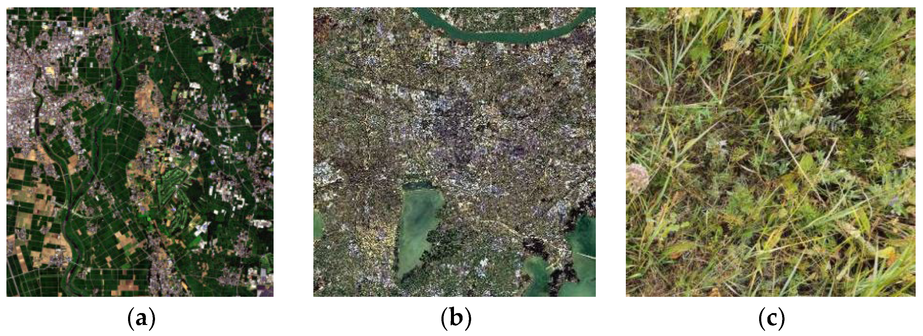
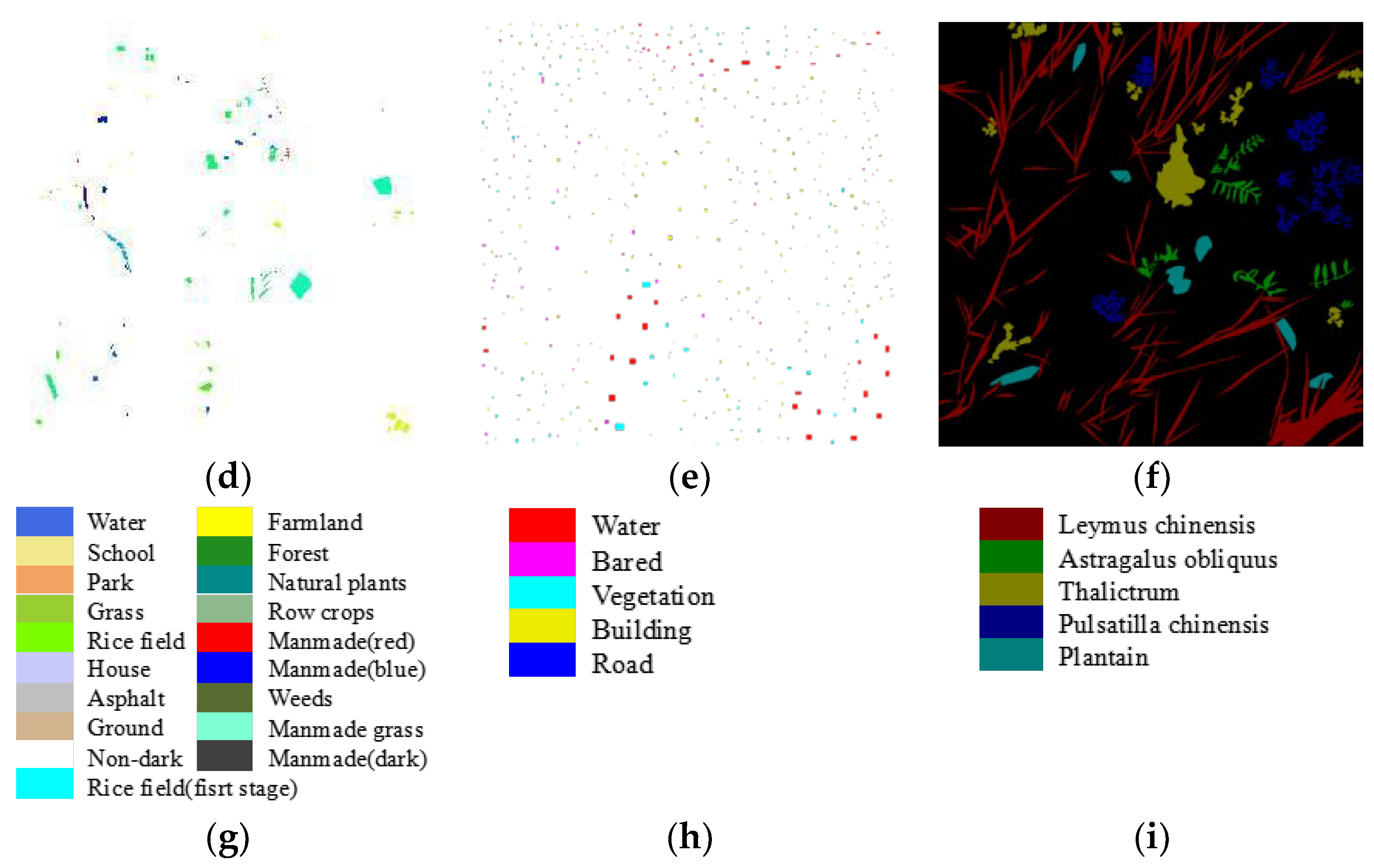
The datasets employed in this study are first introduced. The derivation of the proposed method is then described in detail.

3.1. Datasets

This study conducted validation using three different RSI datasets to verify the effectiveness of the proposed method in the weak information mining of RSIs, and the description of the three datasets is as follows:

(1) Chikusei dataset (CK dataset) [51]: The CK dataset was achieved using the Headwall Hyperspec-VNIR-C imaging sensor over agricultural and urban areas in Chikusei, Ibaraki, Japan (Figure 2a). The image in the CK dataset comprises 2517 × 2335 pixels and contains 128 bands, its spectral range is from 363 nm to 1018 nm, and its spatial resolution is 2.5 m. The ground truth (GT) has 19 classes (including urban and rural areas) and was collected via field survey and visual inspection using high-resolution color images obtained using a Canon EOS 5D Mark II together with the hyperspectral data.

(2) ZY1-02D dataset (ZY dataset) [52]: The ZY dataset was achieved using the hyperspectral sensor on the ZY1-02D satellite in Changzhou city, China (Figure 2b). This dataset has 166 contiguous bands covering the spectral wavelength range from 0.4 µm to 2.5 µm and comprises 1999 × 2051 pixels. The spatial and spectral resolutions of this dataset are 30 m and 10 nm, respectively. The GT is only divided into five classes (i.e., Water, Bared, Vegetation, Building, and Road), which are visually inspected using a high-resolution multispectral image obtained by the ZY1-02D satellite and field survey, due to the low spatial resolution (around 30 m) of the ZY dataset.

(3) Pasture dataset (PT dataset): The PT dataset was collected in the Hulunbuir grassland using the camera of a Huawei P40 mobile phone. The image in the PT dataset was obtained via vertical photography with a 1.5 m height. The RGB image in the PT dataset comprises 8192 × 6144 pixels. The GT for all RGB images in this dataset was obtained through expert visual interpretation combined with field surveys, leading to the classification of data into 10 categories. For the demands of this study, the used RGB image in the PT dataset only contains five categories (Figure 2c).

The CK dataset was employed to assess the spatial and spectral features using the deep spatial–spectral residual feature (DMSR) and deep spatial–spectral coding feature (DMSC). Additionally, the CK dataset was used to determine the intraclass discrimination capability of DMSR and DMSC in fine classification. The ZY dataset was utilized to evaluate the effectiveness of DMSRs and DMSCs in rough classification and examine the interclass identification capacities of DMSR and DMSC. The CK dataset and ZY dataset contain typical remote sensing images; however, RGB images are also an important source of remote sensing data. Thus, this study also aims to test whether or not the proposed method can be used to analyze RGB images with reasonable performance. Therefore, the PT dataset was utilized to explore the feasibility of extending DMSRE to RGB images.

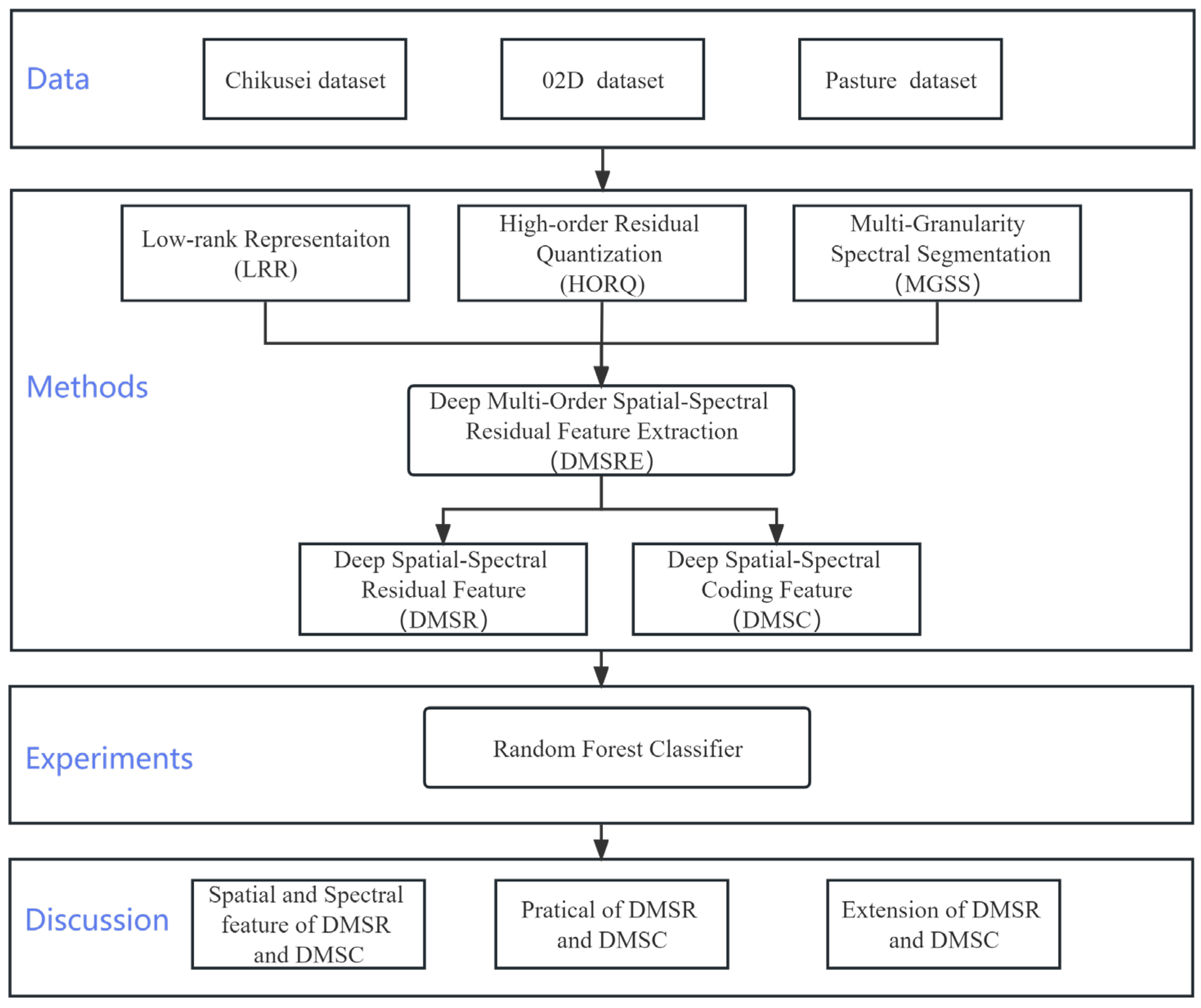
3.2. Deep Multi-Order Spatial–Spectral Residual Feature Extraction

The study aims to develop a spatial–spectral feature extraction technique for mining weak information in RSIs. First, the proposed method tackles the global information within RSIs by converting the three-dimensional structure of raw RSIs into a two-dimensional spatial–spectral information matrix prior to the extraction process. Subsequently, the extracted spatial–spectral features are reorganized into a three-dimensional structure, ensuring dimensional consistency with the raw RSIs. Two sequences of spatial–spectral features are extracted by iteratively decomposing the residuals of the raw RSIs. Figure 3 illustrates the flowchart of the proposed method.

The proposed method extracts spatial–spectral features from RSIs in two directions, at multiple depths, and in various orders (Figure 3) and thus is named deep multi-order spatial–spectral residual feature extraction (DMSRE). DMSRE can extract two sequences of spatial–spectral features with the same dimension of RSIs. The two spatial–spectral feature sequences are referred to as DMSRs and DMSCs. Each sequence of DMSR and DMSC comprises features of multiple orders, with the nth order DMSR or DMSC labeled as the n-order DMSC or DMSR. Furthermore, DMSRE is derived as follows:

Suppose $L$ is a low-rank matrix of the achieved RSI $G$. If the 1st-order DMSR of $L$ is defined as $R{(L)}_1$, then $L$ can be expressed as follows:

$$L=w_1{C}_1+R(L{)}_1,$$

(10)

where $C_1\in {\left\{-1,+1\right\}}^N$ is the coding matrix of $L$ and $w_1$ is the weight of $C_1$. $C_1$ and ${\mathrm{w}}_1$ can generally be calculated as follows:

$$w_1=\frac{1}{mn}{‖L‖}_1,$$

(11)

$$C_1=sign(L).$$

(12)

The $R{\left(L\right)}_1$ in Formula (11) can then be further quantized as follows:

$$R{\left(L\right)}_1=w_2{C}_2+R{\left(L\right)}_2.$$

(13)

Thus, Formula (10) can be rewritten:

$$L=w_1{C}_1+w_2{C}_2+R{\left(L\right)}_2,$$

(14)

where

$$w_2=\frac{1}{mn}{‖R{\left(L\right)}_1‖}_1,$$

(15)

$$C_2=sign(R{(L)}_2).$$

(16)

Moreover, the $R{\left(L\right)}_2$ can be quantized again. Therefore, the $L$ can finally be introduced as follows:

$$L={\displaystyle \sum _{\mathrm{i}}^N{w}_i{C}_i}+R{(L)}_i.$$

(17)

Formula (17) shows that the $R{\left(L\right)}_i$ is close to 0, while the order N is sufficiently high. Thus, Formula (10) can be written as below:

$$L\approx {\sum }_i^N{w}_i{C}_i.$$

(18)

Simultaneously, the analytical solutions of the weighted and coding matrices for each depth are, respectively, presented:

$$w_2=\frac{1}{mn}{‖R{\left(L\right)}_1‖}_1,$$

(19)

$$C_2=sign(R{(L)}_2).$$

(20)

Finally, the DMSC and DMSR can be, respectively, expressed:

$${DMSC}_i={\sum }_i^N{w}_i{c}_i,$$

(21)

$${DMSR}_i=L-{\sum }_i^N{w}_i{c}_i.$$

(22)

Formula (21) shows that the information content of the DMSC sequence features increases with the order until it converges with that of the raw image. Conversely, the information content of DMSR (Formula (22)) decreases as the order increases until it converges to zero. Combining Formulas (21) and (22), the raw RSI can be reconstructed by the same order of DMSR and DMSC.

DMSRE can theoretically extract the feature indefinitely, with the terminated order depending on the raw RSI and its application demands. Therefore, the mean spectral angle (MSA) [53] and structural similarity index (SSIM) [54] were introduced to discuss the terminated order. MSA characterizes the spectral similarity between the DMSC and the raw RSI, whereas SSIM represents the structural similarity between the DMSC and the raw RSI. These metrics are defined as follows:

$$SSIM(X,Y)=\frac{(2{\mu }_X{\mu }_Y+C_1)(2{\sigma }_{XY}+C_2)}{({\mu }_X^2+{\mu }_Y^2+C_1)({\sigma }_X^2+{\sigma }_Y^2+C_2)},$$

(23)

$$MSA=\frac{1}{mn}\sum _{i=1}^{mn}\frac{180}{\pi }arccos\frac{X^{T}Y}{‖X‖‖Y‖},$$

(24)

where X and $Y$ denote the raw RSI and DMSC, respectively. Herein, ${\mu }_X$ signifies the mean value of X, ${\mu }_Y$ represents the mean value of $Y$, and ${\sigma }_X^2$ and ${\sigma }_Y^2$ correspond to the variances of X and Y, respectively. ${\sigma }_{XY}$ stands for the covariance between X and Y. Constants $C_1$ and $C_2$ are introduced to ensure numerical stability during computations. In Formula (24), m and n refer to the number of rows and columns of raw RSIs, respectively. The value of SSIM lies in the range [0, 1], where high values indicate high structural similarity between DMSCs and raw RSIs. Conversely, small values for the MSA indicate high spectral similarity.

3.3. Evaluation Metrics

In this study, F1 scores were employed to evaluation the classification results. The F1 score was evaluated based on the recall and precision, which can be expressed as follows:

$$Recall=\frac{TP}{TP+FN},$$

(25)

$$Precision=\frac{TP}{TP+FP},$$

where TP represents true positives, TN true negatives, FP false positives, and FN false negatives. Moreover, the F1 score can be expressed as follows:

$$F1\_score=\frac{2Recall\times Precision}{Recall+Precision}$$

(26)

A higher F1 score indicates a better classification result. The overall accuracy and the classification accuracy of the single class in the classification result were used to evaluate the F1 score.

4. Results

4.1. Experimental Setting

Theoretically, the proposed method can continuously extract features indefinitely based on the raw image. However, the extracted DMSC is slightly changed while the order is high. Moreover, the terminated order varies for different datasets and demands of applications. This study attempts to find the terminated order, which is highly spectrally and spatially similar to the raw CK dataset (Figure 4). Considering the CK dataset as an example, first-order to sixteenth-order DMSCs and DMSRs are extracted from the CK dataset, and the MSA and SSIM values between the DMSC and the raw CK dataset are then calculated (Figure 5).

It can be easily found that the SSIM is closer to 1 while the order is higher than the eighth order, and the MSA is smaller than 0.05 (Figure 5). In this time, the DMSC is highly similar to the raw image in the image structure and spectral domain. Although there were some orders present that were higher (SSIM) and lower (MSA) than the eight order, little changed compared with the eighth-order DMSC. Therefore, considering the computational power and time costs, this study chose the eighth order as the terminal order of the CK dataset.

4.2. Spatial and Spectral Features of DMSR and DMSC

4.2.1. Spatial Features of DMSR and DMSC

The DMSR was obtained by continuously decomposing the residual of raw RSIs, which indicates that the difference between the DMSR and raw image increases with order. Therefore, the spatial visual of the DMSR displays the image darker than the raw CK dataset in the beginning (Figure 6a), the ground objects in the DMSR gradually fragment with high order (Figure 6), and the shape of the ground object cannot be observed in the high order (Figure 6g,h).

The color images of the DMSC for the CK dataset are shown in Figure 6. The figure demonstrates a black color in the first-order DMSC (Figure 7a), which only contains the mean value of L₁ paradigm from the raw CK dataset, and the color varies depending on raw RSIs. The information content of the DMSC gradually increases with the order. High-reflectivity features, such as the roof and bare ground, are emphasized in the second-order DMSC (Figure 7b). Vegetation such as farmland is highlighted in the third-order DMSC (Figure 7c). Most ground objects are displayed in the fourth-order DMSC (Figure 7d) and are visually increasingly similar to the raw image. Two detailed areas were selected and enlarged to perform a detailed analysis to further understand the DMSR and DMSC trend, as shown in Figure 8.

Detailed image 1 shows the change in the DMSC with order (Figure 8b–i). The figure reveals a black color at the first-order DMSC (Figure 8b), the high-reflectivity features (e.g., roof) are displayed in the second order (Figure 8c), the vegetation (e.g., grassland) is emphasized in the third order, the outline of most classes was recognized but without intraclass information in the fourth order (Figure 8d), and the intraclass information was refined when the order was higher than the fifth order (Figure 8f–i).

Detailed image 2 is used to demonstrate the change in the DMSR with order (Figure 8k–r). The shapes of surface features show a tendency toward gradual fragmentation. The DMSR is visually similar to the raw image in the first order (Figure 8k), the features (e.g., roof) start to be gradually fragmented in the second order (Figure 8l), the weak information has been gradually reflected when the order is higher than third order (Figure 8m); for example, the information in the red box (Figure 8k–o), which is the shadow of the cloud on the ground, is difficult to distinguish from the surrounding grass. However, the surrounding information in the third order to fifth order (Figure 8m–o) demonstrates the capability of the DMSR to mine weak information in RSIs. Overall, the results indicate that the DMSC is appropriate for rough classification, whereas the DMSR is better suited for fine classification. The DMSC and DMSR have the potential to enhance the accuracy of remote sensing classification.

4.2.2. Spectral Features of DMSR

This study extracted the spectral features of vegetation in the DMSC and DMSR as an example for analysis. The spectral curves are displayed in Figure 9.

In Figure 9, the blue curve is the spectral feature achieved from a raw RSI, while the purple and green curves represent the curves of the DMSR and DMSC, respectively. The DMSC shows a straight line in the first order (green line in Figure 9a), which only contains the average value of its L₁ paradigm value. The second-order DMSC (Figure 9b) illustrates the low-reflectivity features (e.g., vegetation) in visible spectral (0.37–0.71 µm) and high-reflectivity features in near-infrared spectral. The first- and second-order DMSCs only retain minimal spectral information of raw RSIs, and the detailed spectral information of the DMSC improves as the order increases (Figure 9c–h), bringing it close to raw RSIs.

On the contrary, the first-order DMSR (purple curve in Figure 9a) maintains all spectral information but is only small in terms of spectral value because the first-order DMSR represents the raw RSIs minus its L₁ paradigm value. The second-order DMSR (Figure 8b) highlights detailed information in the red edge spectral (approximately 0.7 μm wavelength). The DMSR has increased spectral information in the first and second order, and the detailed information becomes rich while the order becomes high (Figure 9b–h). Additionally, as the order increases, the spectral value of the DMSR tends toward 0, while that of the DMSC approaches the raw RSI’s.

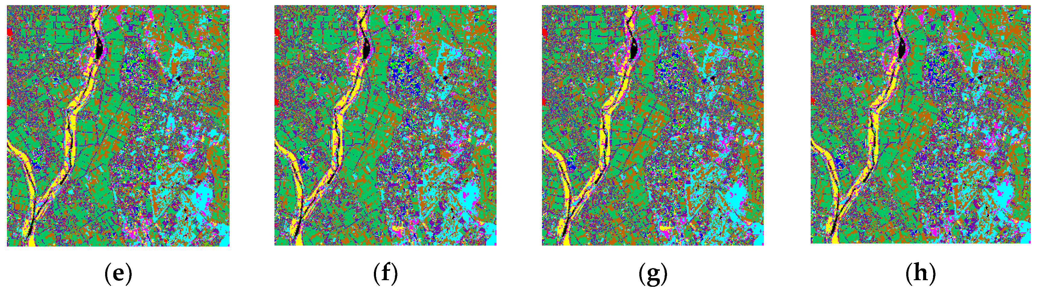
4.3. Classification Results Using DMSR and DMSC

This study performed classification experiments on raw RSIs and their extracted DMSR and DMSC from three RSI datasets via random forest (RF) classifier to verify the performance of the DMSC and DMSR. The CK dataset was applied for fine classification, while the ZY dataset was applied for rough classification. The classification accuracy of each single class and the overall accuracy were obtained from these classification results. High values indicate superior classification results. Figure 10 and Figure 11 illustrate the classification results for the DMSC and DMSR of the CK dataset, respectively.

The classification results using the DMSR (Figure 10) show minimal visual variation. However, significantly more misclassifications are observed while the orders are higher than the fifth order (Figure 10e–h). By contrast, the classification results via DMSC (Figure 11) gradually increase the number of recognized classes as the order rises, and most classes have been recognized while the orders are greater than the fifth order (Figure 11e–h). The classification and overall accuracies were calculated and are listed in

Table 1. Classification accuracy of different-order DMSRs of the CK dataset.

Class Name	Raw	First Order	Second Order	Third Order	Fourth Order	Fifth Order	Sixth Order	Seventh Order	Eighth Order
Water	0.9939	0.9951	0.9916	0.9926	0.9939	0.9924	0.9754	0.9395	0.9402
School	0.9899	0.9850	0.9931	0.9855	0.9720	0.9483	0.9257	0.8300	0.7782
Park	0.7860	0.7146	0.8253	0.7566	0.5662	0.1176	0.5160	0.0000	0.0156
Farmland	0.9880	0.9826	0.9891	0.9847	0.9779	0.9630	0.9604	0.9446	0.9200
Plants	0.9935	0.9879	0.9895	0.9922	0.9893	0.9924	0.9849	0.9817	0.9834
Weeds	0.9704	0.9541	0.9530	0.9681	0.9626	0.9467	0.8929	0.9016	0.9045
Forest	0.9983	0.9962	0.9962	0.9951	0.9883	0.9857	0.9800	0.9742	0.9670
Grass	0.9953	0.9926	0.9957	0.9959	0.9948	0.9891	0.9772	0.9692	0.9611
Rice field (grown)	0.9987	0.9975	0.9978	0.9945	0.9847	0.9789	0.9739	0.9652	0.9539
Rice field	0.9951	0.9991	0.9973	0.9900	0.9913	0.9863	0.9842	0.9584	0.9689
Row crops	0.9971	0.9945	0.9936	0.9964	0.9947	0.9931	0.9846	0.9742	0.9570
House	0.9686	0.9794	0.9791	0.9687	0.9265	0.8136	0.7306	0.5956	0.5482
Manmade	0.9834	0.9834	0.9871	0.9680	0.9148	0.8597	0.8416	0.8203	0.8099
Manmade (dark)	0.9893	0.9942	0.9927	0.9928	0.9926	0.9885	0.9827	0.9723	0.9712
Manmade (Red)	1.0000	0.9935	0.9868	0.9987	0.9564	0.8688	0.7524	0.5589	0.2982
Manmade (Blue)	0.9950	0.9928	0.9700	0.9199	0.9258	0.8371	0.0741	0.0000	0.0000
Manmade grass	0.9879	0.9873	0.9914	0.9835	0.9756	0.9001	0.8633	0.6983	0.5340
Asphalt	0.8912	0.9599	0.9511	0.9456	0.9391	0.9151	0.8593	0.5614	0.4500
Ground	0.9339	0.9153	0.8279	0.8851	0.8185	0.8302	0.0876	0.0000	0.0000
Overall accuracy	0.9922	0.9913	0.9921	0.9902	0.9824	0.9708	0.9570	0.9324	0.9177

and

Table 2. Classification accuracy of different-order DMSCs of the CK dataset.

Class Name	Raw	First Order	Second Order	Third Order	Fourth Order	Fifth Order	Sixth Order	Seventh Order	Eighth Order
Water	0.9939	0.0000	0.0000	0.8549	0.8526	0.9711	0.9913	0.9920	0.9931
School	0.9899	0.0000	0.0000	0.9290	0.9826	0.9868	0.9905	0.9941	0.9920
Park	0.7860	0.0000	0.0000	0.0000	0.3573	0.6038	0.6798	0.6699	0.7229
Farmland	0.9880	0.0000	0.0000	0.9503	0.9620	0.9785	0.9787	0.9825	0.9833
Plants	0.9935	0.0000	0.8034	0.9634	0.9829	0.9896	0.9890	0.9941	0.9927
Weeds	0.9704	0.0000	0.0020	0.8749	0.9250	0.9456	0.9401	0.9590	0.9584
Forest	0.9983	0.4184	0.7992	0.9250	0.9688	0.9936	0.9942	0.9963	0.9968
Grass	0.9953	0.0000	0.7099	0.9819	0.9926	0.9944	0.9942	0.9964	0.9945
Rice field (grown)	0.9987	0.0000	0.7530	0.8947	0.9574	0.9930	0.9943	0.9962	0.9976
Rice field	0.9951	0.0000	0.0000	0.9885	0.9851	0.9965	0.9961	0.9965	0.9978
Row crops	0.9971	0.0000	0.3128	0.9617	0.9838	0.9919	0.9937	0.9928	0.9920
House	0.9686	0.0000	0.1283	0.8995	0.9691	0.9748	0.9782	0.9760	0.9836
Manmade	0.9834	0.0000	0.9656	0.9781	0.9819	0.9813	0.9858	0.9890	0.9843
Manmade (dark)	0.9893	0.0000	0.4234	0.9450	0.9485	0.9855	0.9920	0.9915	0.9931
Manmade (Red)	1.0000	0.0000	0.3644	0.9948	1.0000	1.0000	1.0000	0.9924	0.9963
Manmade (Blue)	0.9950	0.0000	0.8034	0.9624	1.0000	1.0000	0.9950	0.9926	0.9949
Manmade grass	0.9879	0.0000	0.1353	0.8688	0.9821	0.9877	0.9875	0.9846	0.9874
Asphalt	0.8912	0.0000	0.0000	0.6562	0.9253	0.9508	0.9297	0.9384	0.9488
Ground	0.9339	0.0000	0.0000	0.0000	0.5400	0.8787	0.7019	0.8664	0.7500
Overall accuracy	0.9922	0.2645	0.5839	0.6684	0.9625	0.9870	0.9890	0.9911	0.9917

, respectively, based on the classification results of the DMSR and DMSC.

Table 1 provides the classification accuracy of single class and the overall accuracy of classification results; the F1 score was used to assess classification result both of overall accuracy and the single class (the same applies to the following content). The overall accuracy of the DMSR classification result displays a minor decrease as the order increases. However, several individual classes achieved higher classification accuracy than the raw image (highlighted in blue in Table 1), because the weak information related those classes had been mined in the DMSR. The above conclusion supports that the DMSR can improve the accuracy of individual class in fine classification application.

Table 2 shows the accuracy of classification results via DMSC. The overall accuracy demonstrates an increasing trend with the orders. Notably, there are many 0 values in classification results via the first- and second-order DMSC, because first- and second-order DMSCs contain little RSI information. Compared with the classification results of the raw image, the overall accuracy of the DMRC (especially orders higher than the sixth order) only has minor differences. Meanwhile, the rough classification experiment was conducted on the ZY dataset. The classification results via DMSR and DMSC of the ZY dataset are shown in Figure 12 and Figure 13, respectively.

The classification results by first- and second-order DMSR (Figure 12a,b, respectively) can identify the most classes. The number of recognized classes slowly diminishes starting from the third order (Figure 12c), whereas the changes in recognized classes be-come less pronounced after the fifth-order DMSR (Figure 12e). The classification results via first-order DMSC (Figure 13a) only identified the water class, that is, the number of the identified classes with an increasing number as the order increases, from a visual perspective. The changes become less pronounced after the fifth order (Figure 13e). The accuracy of the DMSR and DMSC for the ZY dataset is listed in

Table 3. Classification accuracy of first-order to eighth-order DMSR of the ZY dataset.

Class Name	Raw	First Order	Second Order	Third Order	Fourth Order	Fifth Order	Sixth Order	Seventh Order	Eighth Order
Water	0.9546	0.9548	0.9567	0.9728	0.9756	0.9699	0.9367	0.8174	0.7897
Building	0.9672	0.968	0.9769	0.9852	0.994	0.966	0.9971	0.9969	0.9971
Naked	0.8373	0.8332	0.8005	0.6752	0.5353	0.3094	0.2881	0.1958	0.1892
Vegetation	0.9006	0.8998	0.8423	0.8164	0.9792	0.5321	0.4971	0.4434	0.4377
Road	0.8131	0.7992	0.7636	0.64	0.1454	0.5321	0.089	0.0346	0.0277
Overall accuracy	0.9207	0.9197	0.9016	0.8775	0.81081	0.73134	0.7096	0.645	0.6345

and

Table 4. Classification accuracy of first-order to eighth-order DMSC of the ZY dataset.

Class Name	Raw	First Order	Second Order	Third Order	Fourth Order	Fifth Order	Sixth Order	Seventh Order	Eighth Order
Water	0.9546	0.8261	0.9758	0.9764	0.9853	0.9709	0.9683	0.9616	0.9628
Building	0.9672	1	0.8559	0.9492	0.9629	0.9642	0.9683	0.9683	0.9666
Naked	0.8373	0	0.7779	0.8295	0.8334	0.8342	0.9339	0.8321	0.8359
Vegetation	0.9006	0	0.8081	0.8537	0.8777	0.8882	0.8975	0.9003	0.8961
Road	0.8131	0	0.2423	0.6855	0.7507	0.8002	0.8061	0.8101	0.8051
Overall accuracy	0.9207	0.5015	0.8514	0.9062	0.9204	0.9205	0.9232	0.9278	0.9213

, respectively.

The Water and Building class in the ZY dataset can achieve high accuracy in the classification via DMSR (Table 3): the accuracy of Water improved from 95.46% to 97.56%, while that of Building improved from 96.72% to 99.71%. The overall accuracy in the classification via DMSC (Table 4) achieved a superior result, and the overall accuracy improved from 92.07% to 92.78%. This phenomenon is attributed to the DMSC’s emphasis on highlighting object boundaries by disregarding local detailed information. Consequently, the DMSC tends to yield superior results for rough classification. The DMSC theoretically has potential for improvement in overall accuracy. Furthermore, this study conducts experiments on RGB images in the PT dataset to discuss the scalability of DMSRE. Figure 14 and Figure 15 display the color image of the DMSR and DMSC, respectively.

The spatial variations in DMSR (Figure 14) and DMSC (Figure 15) of the PT dataset are consistent with those in the DMSR and DMSC in the CK and ZY datasets. The amount of information for the DMSR gradually reduces as the orders increase. The first-order DMSR (Figure 14a) only demonstrates a slight decrease in brightness. The difference between the raw image and the DMSR grows larger starting from the Fifth order (Figure 14e). From the fifth to eighth order (Figure 14e–h), only the goat grass feature remains. In the first-order DMSC (Figure 15a), the image is monochromatic, and the DMSC tends to be close to the raw image as the order increases. The classification accuracies of the DMSR and DMSC are presented in

Table 5. Classification accuracy of first- to eighth-order DMSR of the PT dataset.

Class Name	Raw	First Order	Second Order	Third Order	Fourth Order	Fifth Order	Sixth Order	Seventh Order	Eighth Order
Leymus chinensis	0.7684	0.7673	0.7651	0.7635	0.7617	0.7616	0.7607	0.7607	0.7594
Astragalus obliquus	0.2955	0.3189	0.2842	0.2727	0.2042	0.1915	0.1124	0.1180	0.0362
Thalictrum	0.1039	0.1385	0.1040	0.0994	0.0900	0.0980	0.0679	0.0741	0.0275
Pulsatilla chinensis	0.2866	0.2891	0.2485	0.2711	0.2269	0.2118	0.1879	0.1833	0.1584
Plantain	0.3249	0.3986	0.3508	0.3747	0.3440	0.3495	0.2896	0.2960	0.2160
Overall accuracy	0.6325	0.64	0.6243	0.6128	0.6114	0.6113	0.6118	0.6115	0.6112

and

Table 6. Classification accuracy of first- to eighth-order DMSC of the PT dataset.

Class Name	Raw	First Order	Second Order	Third Order	Fourth Order	Fifth Order	Sixth Order	Seventh Order	Eighth Order
Leymus chinensis	0.7684	0.7575	0.7571	0.7581	0.7599	0.7624	0.7633	0.7644	0.7661
Astragalus obliquus	0.2955	0	0.0764	0.0759	0.1808	0.2158	0.2985	0.2962	0.2992
Thalictrum	0.1039	0	0	0.0000	0.0020	0.0254	0.0850	0.1114	0.1000
Pulsatilla chinensis	0.2866	0	0	0.0560	0.1434	0.2036	0.2718	0.2709	0.2743
Plantain	0.3249	0	0	0.0000	0.0640	0.1910	0.3143	0.3303	0.3192
Overall accuracy	0.6325	0.6096	0.6097	0.6109	0.6173	0.6247	0.6321	0.6343	0.6360

, respectively.

From the classification result via raw image, it can be found that the classification accuracy was not higher; only “Leymus chinensis” achieved higher accuracy, and other classes had lower accuracy. This is because “Leymus chinensis” is the main dominant species in the study area, and the other classes are companion species, which means the “Leymus chinensis” class accounted for a large proportion in the PT dataset and other classes had less proportion. Therefore, “Leymus chinensis” easily achieved a higher classification result than other classes. However, it still shows difficulty in companion species classification, and the classification results via DMSR show the potential for this task. In the classification results via DMSR (Table 5), most classes attain higher accuracy than the classification result of the raw image, excluding the “Leymus chinensis” class. However, it improved the classification accuracy of companion species slightly, which also means it has potential for species classification. The overall accuracy performance in the DMSC coincides with the results observed in the two other RSI datasets (Table 6). The overall accuracy steadily improved with the increase in orders, ultimately exceeding the overall accuracy of the raw image.

5. Discussion

5.1. Research Contributions

The main contribution of this study is as follows: First, this study proposes a deep multi-order spatial–spectral feature extraction method that adaptively extracts spatial–spectral features of RSIs from two directions, which does not need training samples. The proposed method further ensures that the extracted feature does not reduce in dimension compared with the raw RSIs because it considers the comprehensive global spatial–spectral information of the RSIs to achieve optimal results. Second, the proposed method can enhance the feature recognition capability of RGB images, demonstrating the universality of the approach. This method is not only applicable to HSI but also to RGB images.

Based on the concept of weak information extraction from RSIs, MGSS [44] was recently developed to facilitate spectral multifeatured weak information extraction technology, specifically for feature extraction in the spectral dimension. The extracted features can be effectively quantified to estimate accuracy, and research has shown certain success in quantitative applications, such as the estimation of forage aboveground biomass [45] and grass crude protein [44], and the monitoring of soil salinity [10].

However, MGSS is limited to achieving good performance in the spectral dimension and cannot be applied to the image dimension. However, information mining using MGSS in RSIs is yet to be explored further. The proposed method is based on LRR, MGSS, and HORQ theories. The extracted DMSRs and DMSCs possess unique properties. The DMSR calculates residuals of the raw image step by step, focusing on weak spatial–spectral information. By contrast, the DMSC highlights interclass boundary information by progressively accumulating the product of coding matrices and magnitudes in the convergence of the raw image. Moreover, this study employed remote sensing classification application to test their properties to effectively understand the characteristics of the DMSR and DMSC. Notably, this finding does not imply that the two features are exclusive to classification applications; rather, they have the potential to have a good performance in qualitative and quantitative applications for the purpose of weak information mining.

5.2. Limitation and Potential Future Work

This study proposed the DMSRE method for the spatial–spectral feature extraction of RSIs. However, DMSRE has certain limitations. While its mathematical foundations have been established, certain gaps in the understanding of its underlying mechanisms exist. Particularly, at lower orders, DMSRE constitutes the dominant factor in the image, yet the specific information represented by each order remains uncertain. For instance, similar to the tasseled cap transformation [55], which explicitly defines the first, second, and third components as brightness, greenness, and wetness, respectively, a similar comprehensive interpretation for DMSRE is still lacking. Furthermore, the investigation into the amplitude values (denoted as “w”) in the DMSCs of RSIs requires further exploration. This issue has also been addressed in the work of Kang [44], signifying the ongoing need for additional in-depth research in this area. Moreover, to fully consider spatial–spectral characteristics, this study handles spatial features in one dimension. The extraction of multidimensional spatial–spectral features is possible, as it also handles some spatial features to some extent; thus, the discussion of its practicality and universality for other applications should be conducted in an actual RS task in the near future. For a similar problem, Truong et al. [56] extracted spatiotemporal features with deep learning for land cover classification, and achieved a high-accuracy land cover classification. Therefore, we will focus on how to use the extracted features to improve the application performance in the next work.

The DMSR and DMSC exhibit distinct characteristics and hold varying application potentials in remote sensing. This investigation not only delves into their potential in classification but also acknowledges their possible promising prospects in remote sensing estimation and inversion due to the DMSR’s weak information extraction capabilities.

6. Conclusions

This study considers the three-dimensional structural properties and global information of RSIs, and without training samples during FE process, this study proposed an adaptive DMSRE method based on LRR, MGSS, and HORQ that can extract features of RSIs in two directions (DMSRs and DMSCs). Classification experiments with DMSRs and DMSCs from three datasets (CK, ZY, and PT datasets) with different attributes showed that the DMSR can improve the classification accuracy of individual classes in fine classification applications, and the DMSC can improve the overall accuracy in rough classification applications. Moreover, the proposed method is not only applicable to HSI but extends to remote sensing RGB images, which has the potential to promote the RSI processing of weak extracted information, and then extend the application of RSIs in different fields.

References

1. Shen, H.; Li, X.; Cheng, Q.; Zeng, C.; Yang, G.; Li, H.; Zhang, L. Missing Information Reconstruction of Remote Sensing Data: A Technical Review. IEEE Geosci. Remote Sens. Mag. 2015, 3, 61–85. [Google Scholar] [CrossRef]
2. Qin, P.; Cai, Y.; Liu, J.; Fan, P.; Sun, M. Multilayer Feature Extraction Network for Military Ship Detection from High-Resolution Optical Remote Sensing Images. IEEE J. Sel. Top. Appl. Earth Obs. Remote Sens. 2021, 14, 11058–11069. [Google Scholar] [CrossRef]
3. Shirmard, H.; Farahbakhsh, E.; Müller, R.D.; Chandra, R. A Review of Machine Learning in Processing Remote Sensing Data for Mineral Exploration. Remote Sens. Environ. 2022, 268, 112750. [Google Scholar] [CrossRef]
4. Chen, H.; Qi, Z.; Shi, Z. Remote Sensing Image Change Detection with Transformers. IEEE Trans. Geosci. Remote Sens. 2022, 60, 5607514. [Google Scholar] [CrossRef]
5. Ozdogan, M.; Yang, Y.; Allez, G.; Cervantes, C. Remote Sensing of Irrigated Agriculture: Opportunities and Challenges. Remote Sens. 2010, 2, 2274–2304. [Google Scholar] [CrossRef]
6. Yu, S.; De Backer, S.; Scheunders, P. Genetic Feature Selection Combined with Composite Fuzzy Nearest Neighbor Classifiers for High-Dimensional Remote Sensing Data. In Proceedings of the SMC 2000 International Conference on Systems, Man and Cybernetics. “Cybernetics Evolving to Systems, Humans, Organizations, and their Complex Interactions” (Cat. No.00CH37166), Nashville, TN, USA, 8–11 October 2000; Volume 3, pp. 1912–1916. [Google Scholar]
7. Bhuvaneswari, K.; Dhamotharan, R.; Radhakrishnan, N. Information Extraction from Remote Sensing Image (RSI) for a Coastal Environment Along a Selected Coastline of Tamilnadu. IJCSET Board Memb. 2011, 95. [Google Scholar]
8. Han, W.; Li, J.; Wang, S.; Wang, Y.; Yan, J.; Fan, R.; Zhang, X.; Wang, L. A Context-Scale-Aware Detector and a New Benchmark for Remote Sensing Small Weak Object Detection in Unmanned Aerial Vehicle Images. Int. J. Appl. Earth Obs. Geoinf. 2022, 112, 102966. [Google Scholar] [CrossRef]
9. Sun, Y.; Cai, W.; Shao, X. Chemometrics: An Excavator in Temperature-Dependent Near-Infrared Spectroscopy. Molecules 2022, 27, 452. [Google Scholar] [CrossRef]
10. Fan, X.; Kang, X.; Gao, P.; Zhang, Z.; Wang, J.; Zhang, Q.; Zhang, M.; Ma, L.; Lv, X.; Zhang, L. Soil Salinity Estimation in Cotton Fields in Arid Regions Based on Multi-Granularity Spectral Segmentation (MGSS). Remote Sens. 2023, 15, 3358. [Google Scholar] [CrossRef]
11. Wang, J.; Zhen, J.; Hu, W.; Chen, S.; Lizaga, I.; Zeraatpisheh, M.; Yang, X. Remote Sensing of Soil Degradation: Progress and Perspective. Int. Soil Water Conserv. Res. 2023, 11, 429–454. [Google Scholar] [CrossRef]
12. Abdollahi, A.; Pradhan, B.; Shukla, N.; Chakraborty, S.; Alamri, A. Deep Learning Approaches Applied to Remote Sensing Datasets for Road Extraction: A State-Of-The-Art Review. Remote Sens. 2020, 12, 1444. [Google Scholar] [CrossRef]
13. Rasti, B.; Hong, D.; Hang, R.; Ghamisi, P.; Kang, X.; Chanussot, J.; Benediktsson, J.A. Feature Extraction for Hyperspectral Imagery: The Evolution from Shallow to Deep: Overview and Toolbox. IEEE Geosci. Remote Sens. Mag. 2020, 8, 60–88. [Google Scholar] [CrossRef]
14. Ebied, H.M. Feature Extraction Using PCA and Kernel-PCA for Face Recognition. In Proceedings of the 2012 8th International Conference on Informatics and Systems (INFOS), Giza, Egypt, 14–16 May 2012; p. MM-72. [Google Scholar]
15. Aliyari Ghassabeh, Y.; Rudzicz, F.; Moghaddam, H.A. Fast Incremental LDA Feature Extraction. Pattern Recognit. 2015, 48, 1999–2012. [Google Scholar] [CrossRef]
16. Prasad, S.; Bruce, L.M. Limitations of Principal Components Analysis for Hyperspectral Target Recognition. IEEE Geosci. Remote Sens. Lett. 2008, 5, 625–629. [Google Scholar] [CrossRef]
17. Kumar, B.; Dikshit, O.; Gupta, A.; Singh, M.K. Feature Extraction for Hyperspectral Image Classification: A Review. Int. J. Remote Sens. 2020, 41, 6248–6287. [Google Scholar] [CrossRef]
18. Ye, Z.; Bai, L.; He, M. Review of Spatial-Spectral Feature Extraction for Hyperspectral Image. J. Image Graph. 2021, 26, 1737–1763. [Google Scholar]
19. Candès, E.J.; Li, X.; Ma, Y.; Wright, J. Robust Principal Component Analysis? J. ACM 2011, 58, 1–37. [Google Scholar] [CrossRef]
20. Zou, H.; Hastie, T.; Tibshirani, R. Sparse Principal Component Analysis. J. Comput. Graph. Stat. 2006, 15, 265–286. [Google Scholar] [CrossRef]
21. Yang, J.; Yang, J. Why Can LDA Be Performed in PCA Transformed Space? Pattern Recognit. 2003, 36, 563–566. [Google Scholar] [CrossRef]
22. Bandos, T.V.; Bruzzone, L.; Camps-Valls, G. Classification of Hyperspectral Images with Regularized Linear Discriminant Analysis. IEEE Trans. Geosci. Remote Sens. 2009, 47, 862–873. [Google Scholar] [CrossRef]
23. Du, Q. Modified Fisher’s Linear Discriminant Analysis for Hyperspectral Imagery. IEEE Geosci. Remote Sens. Lett. 2007, 4, 503–507. [Google Scholar] [CrossRef]
24. Tipping, M.E.; Bishop, C.M. Probabilistic Principal Component Analysis. J. R. Stat. Soc. Ser. B Stat. Methodol. 1999, 61, 611–622. [Google Scholar] [CrossRef]
25. Liang, Z.; Xia, S.; Zhou, Y. Normalized Discriminant Analysis for Dimensionality Reduction. Neurocomputing 2013, 110, 153–159. [Google Scholar] [CrossRef]
26. He, X.; Niyogi, P. Locality Preserving Projections. Adv. Neural Inf. Process. Syst. 2003, 16. [Google Scholar]
27. Cai, D.; He, X.; Wang, X.; Bao, H.; Han, J. Locality Preserving Nonnegative Matrix Factorization. In Proceedings of the Twenty-First International Joint Conference on Artificial Intelligence, Pasadena, CA, USA, 11–17 July 2009. [Google Scholar]
28. Lee, D.D.; Seung, H.S. Learning the Parts of Objects by Non-Negative Matrix Factorization. Nature 1999, 401, 788–791. [Google Scholar] [CrossRef] [PubMed]
29. Berge, A.; Solberg, A.S. Structured Gaussian Components for Hyperspectral Image Classification. IEEE Trans. Geosci. Remote Sens. 2006, 44, 3386–3396. [Google Scholar] [CrossRef]
30. Bhagavathy, S.; Manjunath, B.S. Modeling and Detection of Geospatial Objects Using Texture Motifs. IEEE Trans. Geosci. Remote Sens. 2006, 44, 3706–3715. [Google Scholar] [CrossRef]
31. Pesaresi, M.; Benediktsson, J.A. A New Approach for the Morphological Segmentation of High-Resolution Satellite Imagery. IEEE Trans. Geosci. Remote Sens. 2001, 39, 309–320. [Google Scholar] [CrossRef]
32. Melgani, F.; Serpico, S.B. A Markov Random Field Approach to Spatio-Temporal Contextual Image Classification. IEEE Trans. Geosci. Remote Sens. 2003, 41, 2478–2487. [Google Scholar] [CrossRef]
33. Akcay, H.G.; Aksoy, S. Automatic Detection of Geospatial Objects Using Multiple Hierarchical Segmentations. IEEE Trans. Geosci. Remote Sens. 2008, 46, 2097–2111. [Google Scholar] [CrossRef]
34. Mallinis, G.; Koutsias, N.; Tsakiri-Strati, M.; Karteris, M. Object-Based Classification Using Quickbird Imagery for Delineating Forest Vegetation Polygons in a Mediterranean Test Site. ISPRS J. Photogramm. Remote Sens. 2008, 63, 237–250. [Google Scholar] [CrossRef]
35. Fauvel, M.; Tarabalka, Y.; Benediktsson, J.A.; Chanussot, J.; Tilton, J.C. Advances in Spectral-Spatial Classification of Hyperspectral Images. Proc. IEEE 2012, 101, 652–675. [Google Scholar] [CrossRef]
36. Benediktsson, J.A.; Palmason, J.A.; Sveinsson, J.R. Classification of Hyperspectral Data from Urban Areas Based on Extended Morphological Profiles. IEEE Trans. Geosci. Remote Sens. 2005, 43, 480–491. [Google Scholar] [CrossRef]
37. Kang, X.; Li, S.; Benediktsson, J.A. Feature Extraction of Hyperspectral Images with Image Fusion and Recursive Filtering. IEEE Trans. Geosci. Remote Sens. 2014, 52, 3742–3752. [Google Scholar] [CrossRef]
38. LeCun, Y.; Bengio, Y.; Hinton, G. Deep Learning. Nature 2015, 521, 436–444. [Google Scholar] [CrossRef] [PubMed]
39. Chen, Y.; Jiang, H.; Li, C.; Jia, X.; Ghamisi, P. Deep Feature Extraction and Classification of Hyperspectral Images Based on Convolutional Neural Networks. IEEE Trans. Geosci. Remote Sens. 2016, 54, 6232–6251. [Google Scholar] [CrossRef]
40. Chen, Y.; Zhao, X.; Jia, X. Spectral–Spatial Classification of Hyperspectral Data Based on Deep Belief Network. IEEE J. Sel. Top. Appl. Earth Obs. Remote Sens. 2015, 8, 2381–2392. [Google Scholar] [CrossRef]
41. Ma, X.; Wang, H.; Geng, J. Spectral–Spatial Classification of Hyperspectral Image Based on Deep Auto-Encoder. IEEE J. Sel. Top. Appl. Earth Obs. Remote Sens. 2016, 9, 4073–4085. [Google Scholar] [CrossRef]
42. Kavitha, M.; Gayathri, R.; Polat, K.; Alhudhaif, A.; Alenezi, F. Performance Evaluation of Deep E-CNN with Integrated Spatial-Spectral Features in Hyperspectral Image Classification. Measurement 2022, 191, 110760. [Google Scholar] [CrossRef]
43. Kang, X.; Zhang, A. A Novel Method for High-Order Residual Quantization-Based Spectral Binary Coding. Spectrosc. Spectr. Anal. 2019, 39, 3013–3020. [Google Scholar]
44. Kang, X.; Zhang, A. Hyperspectral Remote Sensing Estimation of Pasture Crude Protein Content Based on Multi-Granularity Spectral Feature. Trans. Chin. Soc. Agric. Eng 2019, 35, 161–169. [Google Scholar]
45. Kang, X.-Y.; Zhang, A.-W.; Pang, H.-Y. Estimation of Grassland Aboveground Biomass from UAV-Mounted Hyperspectral Image by Optimized Spectral Reconstruction. Spectrosc. Spectr. Anal. 2021, 41, 250–256. [Google Scholar]
46. Pang, H.; Zhang, A.; Yin, S.; Zhang, J.; Dong, G.; He, N.; Qin, W.; Wei, D. Estimating Carbon, Nitrogen, and Phosphorus Contents of West–East Grassland Transect in Inner Mongolia Based on Sentinel-2 and Meteorological Data. Remote Sens. 2022, 14, 242. [Google Scholar] [CrossRef]
47. Li, Z.; Ni, B.; Zhang, W.; Yang, X.; Gao, W. Performance Guaranteed Network Acceleration via High-Order Residual Quantization. In Proceedings of the 2017 IEEE International Conference on Computer Vision (ICCV), Venice, Italy, 22–29 October 2017; pp. 2603–2611. [Google Scholar]
48. Rastegari, M.; Ordonez, V.; Redmon, J.; Farhadi, A. Xnor-Net: Imagenet Classification Using Binary Convolutional Neural Networks; Springer: Berlin/Heidelberg, Germany, 2016; pp. 525–542. [Google Scholar]
49. Courbariaux, M.; Hubara, I.; Soudry, D.; El-Yaniv, R.; Bengio, Y. Binarized Neural Networks: Training Deep Neural Networks with Weights and Activations Constrained to +1 or −1. arXiv 2016, arXiv:1602.02830. [Google Scholar]
50. Liu, G.; Lin, Z.; Yu, Y. Robust Subspace Segmentation by Low-Rank Representation. In Proceedings of the 27th international conference on machine learning (ICML-10), Haifa, Israel, 21–24 June 2010; pp. 663–670. [Google Scholar]
51. Yokoya, N.; Iwasaki, A. Airborne Hyperspectral Data over Chikusei; Technical Report SAL-2016-05-27; Space Application Laboratory, The University of Tokyo: Tokyo, Japan, 2016. [Google Scholar]
52. Zhang, X.; Zhang, A.; Portelli, R.; Zhang, X.; Guan, H. ZY-1 02D Hyperspectral Imagery Super-Resolution via Endmember Matrix Constraint Unmixing. Remote Sens. 2022, 14, 4034. [Google Scholar] [CrossRef]
53. Cao, C.; Yu, J.; Zhou, C.; Hu, K.; Xiao, F.; Gao, X. Hyperspectral Image Denoising via Subspace-Based Nonlocal Low-Rank and Sparse Factorization. IEEE J. Sel. Top. Appl. Earth Obs. Remote Sens. 2019, 12, 973–988. [Google Scholar] [CrossRef]
54. Sara, U.; Akter, M.; Uddin, M.S. Image Quality Assessment through FSIM, SSIM, MSE and PSNR—A Comparative Study. J. Comput. Commun. 2019, 7, 8–18. [Google Scholar] [CrossRef]
55. Zhang, X.; Schaaf, C.B.; Friedl, M.A.; Strahler, A.H.; Gao, F.; Hodges, J.C.F. MODIS Tasseled Cap Transformation and Its Utility. In Proceedings of the IEEE International Geoscience and Remote Sensing Symposium, Toronto, ON, Canada, 24–28 June 2002; Volume 2, pp. 1063–1065. [Google Scholar]
56. Truong, V.T.; Hirayama, S.; Phan, D.C.; Hoang, T.T.; Tadono, T.; Nasahara, K.N. JAXA’s New High-Resolution Land Use Land Cover Map for Vietnam Using a Time-Feature Convolutional Neural Network. Sci. Rep. 2024, 14, 3926. [Google Scholar] [CrossRef]
Figure 1. Flowchart of LRR for RSI.
Remotesensing 16 01957 g001
Figure 2. Color image sample of (a) CK dataset, (b) ZY dataset, (c) PT dataset; corresponding GT of (d) CK dataset, (e) ZY dataset, (f) PT dataset; and corresponding legend of (g) CK dataset, (h) ZY dataset, and (i) PT dataset.
Remotesensing 16 01957 g002aRemotesensing 16 01957 g002b
Figure 3. Flowchart of the proposed method. (DMSR: deep spatial–spectral residual feature; DMSC: deep spatial–spectral coding feature).
Remotesensing 16 01957 g003
Figure 4. Schematic of this study.
Remotesensing 16 01957 g004
Figure 5. SSIM (a) and MSA (b) values between the CK dataset and its DMSC.
Remotesensing 16 01957 g005
Figure 6. Color image of (ah) first- to eighth-order DMSR of the CK dataset.
Remotesensing 16 01957 g006
Figure 7. Color images of (ah) first- to eighth-order DMSC for the CK dataset.
Remotesensing 16 01957 g007
Figure 8. Image of (a) detailed image 1, (bi) first-order to eighth-order of DMSC of detailed image 1, (j) detailed image 2, and (kr) first-order to eighth-order DMSR of detailed image 2.
Remotesensing 16 01957 g008
Figure 9. Spectral (vegetation) features of (ah) the spectral curves of the first-order to eighth-order DMSC and DMSR.
Remotesensing 16 01957 g009
Figure 10. Classification results of (ah) first-order to eighth-order DMSR of the CK dataset.
Remotesensing 16 01957 g010
Figure 11. Classification results of (ah) the first-order to eighth-order DMSC of the CK dataset.
Remotesensing 16 01957 g011aRemotesensing 16 01957 g011b
Figure 12. Classification results of (ah) first-order to eighth-order DMSR of the ZY dataset.
Remotesensing 16 01957 g012aRemotesensing 16 01957 g012b
Figure 13. Classification results of (ah) first-order to eighth-order DMSC of the ZY dataset.
Remotesensing 16 01957 g013
Figure 14. Color image of (ah) first-order to eighth-order DMSR of the PT dataset.
Remotesensing 16 01957 g014
Figure 15. Color image of (ah) first-order to eighth-order DMSC of the PT dataset.
Remotesensing 16 01957 g015aRemotesensing 16 01957 g015b