Abstract
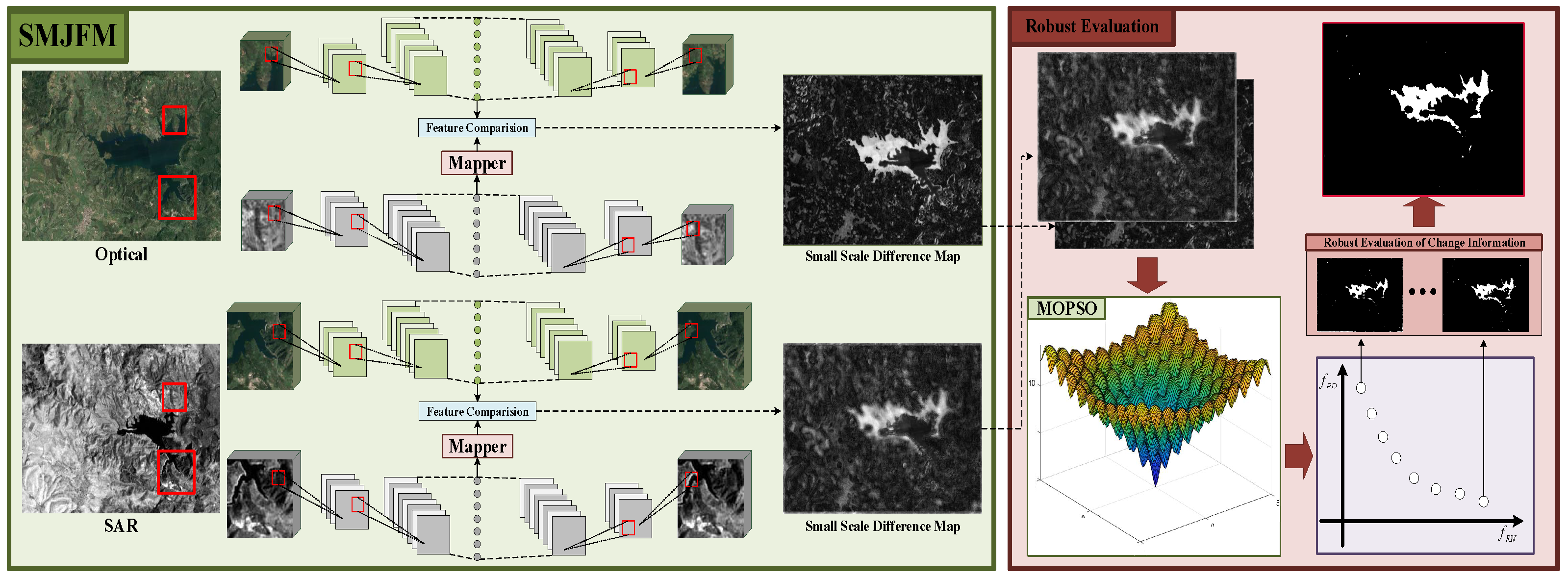
Heterogeneous image change detection is a very practical and challenging task because the data in the original image have a large distribution difference and the labeled samples of the remote sensing image are usually very few. In this study, we focus on solving the issue of comparing heterogeneous images without supervision. This paper first designs a self-paced multi-scale joint feature mapper (SMJFM) for the mapping of heterogeneous data to similar feature spaces for comparison and incorporates a self-paced learning strategy to weaken the mapper’s capture of non-consistent information. Then, the difference information in the output of the mapper is evaluated from two perspectives, namely noise robustness and detail preservation effectiveness; then, the change detection problem is modeled as a multi-objective optimization problem. We decompose this multi-objective optimization problem into several scalar optimization subproblems with different weights, and use particle swarm optimization to optimize these subproblems. Finally, the robust evaluation strategy is used to fuse the multi-scale change information to obtain a high-precision binary change map. Compared with previous methods, the proposed SMJFM framework has the following three main advantages: First, the unsupervised design alleviates the dilemma of few labels in remote sensing images. Secondly, the introduction of self-paced learning enhances SMJFM’s capture of the unchanged region mapping relationship between heterogeneous images. Finally, the multi-scale change information fusion strategy enhances the robustness of the framework to outliers in the original data.
1. Introduction
The process of determining a difference in an object or phenomenon state via observation at various times is known as remote sensing image change detection [1,2,3,4]. Depending on whether or not the image acquisition sources are the same, it is separated into the following two categories: homogeneous image change detection and heterogeneous image change detection. For the study of urban growth, agriculture, forest resources, and disaster assistance, remote sensing image change detection has a strong practical significance [5,6,7,8,9,10,11]. The remote sensing images captured by multiple sensors have huge distribution differences. Therefore, heterogeneous remote sensing images will differ greatly, even within the same scene. For homogeneous images, numerous change detection techniques have been presented under this paradigm [12,13,14,15,16,17,18]. However, because heterogeneous images have different features, applying the homogeneous change detection approach to them directly will not produce adequate results.
Optical and SAR images are the two common types of remote sensing images that we concentrate on in our work. An optical sensor converts the optical signal into an electrical signal, thereby generating an optical image. Compared to optical systems, SAR systems operate on distinct principles. In order to detect objects on the ground, an SAR sensor actively emits radio waves, hears echoes, and uses the echoes it receives to create SAR images. While the forms of the objects and the lighting conditions affect how they seem in optical images, the key determinant of object appearance in SAR images is the item’s reflection qualities [19,20,21]. Optical and SAR images typically exhibit distinct visual properties, making heterogeneous remote sensing image change detection highly valuable in practice. However, the significant differences in data distribution between these two types of remote sensing images pose considerable challenges to this endeavor.
This paper introduces an unsupervised deep learning model, SMJFM, for change detection. SMJFM is based on a multi-scale joint feature mapper (MJFM) with an autoencoder architecture and uses a self-paced learning strategy to assist in optimization, then uses a multi-objective evolutionary algorithm (MOEA) to post-process the model output results. Initially, the approach treats each pixel, along with its surrounding area, as a patch. We define two sizes for the neighborhood—one large and one small—resulting in image patches of varying scales. Correspondingly, two joint feature mappers (JFMs) are constructed to map heterogeneous image patches to a more consistent feature space for feature-level comparison, and the difference information between heterogeneous images is obtained. Usually, the difference information obtained using smaller image patches retains more original image details but introduces more noise information, and the difference information obtained using larger image patches has less noise, but the image is smoother and has less detail information. To balance between noise robustness and detail retention effectiveness, this study incorporates multi-objective optimization to address the challenge. Multi-objective evolutionary algorithms offer the advantage of producing a collection of non-dominated Pareto solutions in a single iteration [22,23]. Finally, the robust evaluation strategy is used to fuse the change information corresponding to multiple Pareto solutions to obtain a high-precision binary change map. Compared with previous threshold methods or clustering methods to deal with difference maps, the robust evaluation strategy fuses the difference map information under different conditions, which improves the robustness of the framework to noise or abnormal data in the original data space.
Considering a pair of heterogeneous images, in order to make the difference map obtained by the joint feature mapper better reflect the difference information of the heterogeneous images, we hope that the JFM focuses on the mapping relationships in the data of the unchanged region and weakly captures the mapping relationships in the data of the changed region. Therefore, in this paper, we introduce a self-paced learning (SPL) strategy to train the JFM. SPL learns training samples from easy to difficult [24]. In heterogeneous remote sensing images, there are usually more unchanged regions than changing regions, and the JFM can usually capture the mapping relationship between unchanged regions more easily, while SPL automatically assigns larger weights to these samples. As for the data of the changed region, its mapping relationship usually contradicts the data of the unchanged region, and self-paced learning assigns smaller weights to these samples, which makes the JFM learn the data mapping relationship between unchanged regions more adequately.
2. Background and Motivation
In this section, we begin with the definition of a remote sensing change detection problem and introduce related work in the field. Then, we introduce the basics of evolutionary multi-objective optimization and some basics of self-paced learning.
2.1. Problem Definition
The aim of heterogeneous image change detection is to detect the change in the same geographical area in two remote sensing images registered at different times. Note that our approach uses two coregistered images, and modest coregistration mistakes would have less of an effect on our approach’s speed because we employ a patch to represent a rather error-tolerant pixel.
2.2. Related Work
Three categories can be distinguished by the numerous research topics and approaches that have been expressed for heterogeneous remote sensing image change detection [22,23,24]. First, several classification-based techniques, including those found in [25,26,27,28,29], such as post-classification comparison (PCC) [30] and classified adversarial networks (CANs) [31], can be used to handle heterogeneous change detection. PCC is a workable method for detecting changes in heterogeneous images. Two heterogeneous photos are segmented according to the different classes of ground objects, and the segmentation result is then used to obtain the change detection result. Such methods are usually simple and practical, but their accuracy is limited by the performance of the classification algorithm and will be affected by the accumulation of classification errors. A CAN employs adversarial training to explore the relationship between heterogeneous data and their corresponding labels. Following training, the heterogeneous data are fed into the generator to generate the final change map. The change detection accuracy of this method is also affected by the classification accuracy, and the training of the generator is a tedious process. In [32], Lv et al. identified potential samples by evaluating the similarity between the initial sample and its neighboring blocks. These potential samples were then used to train the neural network and predict the intermediate results. These operations were integrated through an iterative algorithm to facilitate the training and prediction of the neural network. However, this method involves a training sample enhancement strategy, which is highly dependent on the quality and representativness of the initial samples. If the initial sample is improperly selected, it may affect the entire iterative process. In [33], Li et al. proposed the SSPCN framework by combining adaptive step learning and convolutional networks; the method dynamically selects reliable samples and learns the relationship between two heterogeneous images. Pseudo-labels are initialized using a classification-based approach, and weights are assigned to each sample to represent its tractability. Subsequently, self-paced learning (SPL) prioritizes the learning of easier samples initially, gradually incorporating more complex ones over time. The introduction of the SPL strategy makes this method able to alleviate the phenomenon whereby the accuracy of change detection decreases due to the insufficient performance of classification algorithm. In [34], in order to solve the problem of false positives in heterogeneous image change detection, Xu et al. proposed a change detection method (CGCD) based on a convolutional neural network (CNN) and graph convolutional network (GCN). This method uses a CNN to learn the feature maps of multi-temporal images and calculate the difference maps of different scales so that low-level and high-level features contribute equally to change detection, then uses a GCN to classify the difference maps to obtain the change maps. However, this method uses pseudo-label samples for unsupervised training, and its performance may depend on the quality and accuracy of the pseudo-label samples. Second, some techniques, such those found in [35,36,37,38,39,40] and a symmetric convolutional coupling network (SCCN) [11], combine the two heterogeneous pictures into a similar feature space. Two heterogeneous images are mapped to a feature space using an SCCN, which then compares the images and creates a difference map. The accuracy of the results is dependent on the percentage of unchanged regions in the photos, and the process is unsupervised. An SCCN largely depends on the definition and optimization of the coupling function. If the coupling function does not capture the changes between images well, it may lead to performance degradation. In order to learn local and high-level features from a given pixel’s local neighborhood in an unsupervised manner, SMC+FCA [40] employs a denoising autoencoder. Afterward, the combination of feature similarity analysis and difference map building allows SMC+FCA to determine the change detection result by segmenting the final change map. This method relies on reliable training examples selected from the rough initial change map (ICM). If the quality of the ICM is not high, it may affect the accuracy of the mapping function and the final change detection results. In [41], Wu et al. proposed CACD, which integrates heterogeneous information into feature vectors for comparison and has a certain degree of robustness to noise in remote sensing data. The deep network structure in CACD is simple and easy to train, and the whole process does not contain any special noise reduction algorithm, which simplifies the optimization process of the algorithm. In [42], Xing et al. performed progressive modal alignment (PMA) on heterogeneous remote sensing images to improve the detection accuracy. A pseudo-label self-learning strategy was designed, and the pseudo-label generated in the modal alignment process was used to guide the detection of the change area. The detection results, in turn, refine the pseudo-label. However, this method relies on initialization. In the preheating training phase, the generation of the initial change map has an important impact on the final performance of the model. If the quality of the initial change map is not high, it may affect the convergence of the model and the final detection results. Third, some approaches model the interdependence between two heterogeneous images or the combined statistics using parametric models such as Markov random field (MRF) [43]. MRF relies on an initial iterative estimation method to estimate the parameters of the Markovian mixture model while considering the diversity of laws in the distribution mixture. Subsequently, the change detection map’s maximum a posteriori solution is calculated based on the determined parameters. However, this method is based on some assumptions, such as conditional independent pixel pair data and a specific likelihood distribution. These assumptions may not always hold in practical applications. PCC, SCCN, CAN, CACD, MRF, CGCD, and PMA will be compared with our approach.
2.3. Evolutionary Multi-Objective Optimization
A multi-objective optimization problem (MOP) can be expressed as follows:
where x is the solution of the MOP, is the target space, maps the solution x to the target space, and is the feasible space. The objectives in an MOP are usually conflicting, which means that it is impossible for any point in the feasible space to minimize all objectives at the same time. For minimization, if and only if one solution () is better than another solution (), the following holds:
When there is no solution dominating in the feasible space (), is called the Pareto-optimal solution. We make a series of composed of become the Pareto-optimal vector. The objectives within the Pareto-optimal vector exhibit the following trade-off relationship: decreasing one objective will result in an increase in another objective. All points in the Pareto-optimal set adhere to this principle, collectively forming what is known as the Pareto-optimal frontier (PF) [44].
Evolutionary algorithms have found successful applications in areas such as privacy protection [45], neural architecture search [46], block sparse recovery and reconstruction [47], remote sensing image processing [48], and self-paced learning [49]. Many studies have employed evolutionary algorithms (EAs) to tackle multi-objective problems due to their ability to handle multiple potential solutions simultaneously.
2.4. Self-Paced Learning
Taking inspiration from the human learning process, Bengio et al. introduced the concept of curriculum learning [24]. The intuition comes from the human learning process, and the data are sent into the model in order of difficulty according to prior knowledge. As an improvement of course learning, SPL updates the course through the maturity of the model. To date, SPL has been maturely used in many fields, such as matrix decomposition and consistency detection [50,51,52,53,54,55,56,57,58]. To mitigate the issue of encountering undesirable local minima in matrix decomposition amidst noise and missing data, Zhao et al. tackled the problem by utilizing SPL [57]. Meanwhile, Zhang et al. integrated the multi-instance learning (MIL) problem into an SPL-based approach termed SP-MIL, demonstrating successful application in cosaliency detection [58].
In this article, the training set is , where denotes the nth sample pair. is the JFM, where is the model parameter. Let reflect the loss of the nth sample pair. In SPL, is used to represent the difficulty of the sample, and the model parameters and weight vectors are optimized by Equation (3).
The speed parameter () governs the pace of sample learning, and it is closely linked to the sample’s loss and weight. However, in the absence of any prior knowledge, the determination of the velocity parameter () is a difficult problem. Usually, the aim of a robust parameter () determination method is to sort the loss of the participating training samples in ascending order and determine , where denotes the number of samples used in training and can be conveniently controlled by adjusting the parameter. The self-paced function () profoundly affects the sample weight, and researchers made a variety of variants of the original self-paced function to cope with diverse tasks [54,55].
In the original SPL hard weighting strategy [59], the weight can only be 0 or 1, and the optimal weight is calculated as follows:
According to (4), samples with a loss of less than are considered simple samples for selection. Thus, the speed parameter () governs the quantity of training samples. When is small, the model is relatively “young”, so easy samples are selected for learning. When is large, the model is relatively “mature”. At this time, complex samples are included to promote the attainment of more comprehensive knowledge by the model. It can be easily imagined that when the deep model is trained using a data set with a small number of false labels, when the value of is small, the number of samples in the training queue is small and the sample loss is small, which means that the samples in the training queue are more reliable (i.e., the samples with correct labels). However, due to the small sample size, the model can easily overfit the data in the training queue to reduce the generalization performance. When the value of is large, the data included in the training queue are more complex and diverse, and the mislabeled samples will be included, which will seriously endanger the performance of the deep model. In the SPL process, changes from small to large, and the training queue expands accordingly, which ensures the good performance of the model on reliable samples while taking into account the generalization of the model and suppresses the negative impact of mislabeled samples on model performance.
3. Methodology
In this section, we begin by outlining the specifics of SMJFM and elaborating on the loss function of JFM. Then, we introduce the optimization details of JFM after introducing self-paced learning. Finally, we describe the robust change map evaluation strategy based on Pareto-optimal solutions. The overall algorithm framework is shown in Algorithm 1, and Figure 1 shows the overall framework of SMJFM.
| Algorithm 1 Overall framework of SMJFM |
|
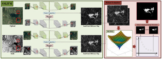
Figure 1.
The overall framework. First, the multi-scale heterogeneous image patches are input into MJFM to obtain two difference maps. Then, the MOPSO optimizes the two objectives of detail preservation and noise suppression. Finally, the final high-precision binary change map is obtained by robustly evaluating the change map corresponding to each Pareto-optimal solution.
| Algorithm 2 Algorithm for MOPSO in remote sensing image change detection |
|
3.1. Multi-Scale Joint Feature Mapper
The joint feature mapper (JFM) is designed based on the architecture of the autoencoder, and the multi-scale is reflected in the size of the input image patch. The specific details of MJFM are shown in Figure 2. MJFM consists of two JFMs. The upper JFM inputs a small-scale patch to compare the difference information of heterogeneous image blocks in more detail. The lower JFM inputs a larger-scale patch to generate a smoother difference map.
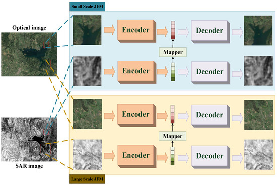
Figure 2.
Illustration of MJFM. The upper JFM inputs small-scale patches, and the lower JFM inputs large-scale patches. The mapper maps the feature vectors of the SAR patches to the feature space closer to the optical patches for comparison.
Each JFM consists of two autoencoders tasked with extracting features from SAR and optical image patches, respectively. The autoencoder maps each image patch to the high-level representation space, and the reconstruction error constraint of the high-level feature vector contains the texture information and spatial information of each image patch.
where denotes the original image patch, and stands for the patch reconstructed by the autoencoder, with and representing the patch size.
Each side of the autoencoder compresses the image patch to a more compact feature vector, and the mapper maps the feature vector on one side to the feature space similar to the other side through feature-level reconstruction constraints. This study maps the features of the SAR image patch.
where is the mapper, and is the feature vector mapped by the mapper.
In summary, the objective function of each JFM is expressed as follows:
where H and W represent the size of the original remote sensing image, while and denote the size of the image patch. denotes the patch consisting of pixels in the ith row and jth column of the SAR image and its neighborhood. Other variables can be derived similarly.
MJFM consists of two JFMs with the same optimization goal and different input patch sizes.
3.2. MJFM with Self-Paced Learning (SMJFM)
In remote sensing image change detection, the count of pixels in the unchanged region typically surpasses the count in the changed region by a significant margin. In addition, the mapping relationship between pixels in the unchanged area is more consistent, and the JFM can more easily capture the mapping relationship of the unchanged area. For the changed region, the mapping relationship between pixels is usually contradictory to the mapping relationship of pixels in the unchanged region and is more complex and diverse. Based on this assumption, this paper integrates self-paced learning into the optimization process of MJFM so that MJFM pays more attention to the mapping relationship of the unchanged region so as to obtain a more significant difference map.
SPL learns samples step by step in the order of learning difficulty (i.e., sample loss). Samples with smaller weights almost do not affect the performance of the network. After introducing SPL into MJFM, the optimization objective is updated as follows:
where N represents the total pixel count, ) is the JFM, and represents the parameter of the JFM.
The SPL model is solved using a majorization–minimization (MM) algorithm. The goal of MM algorithms, which are extensively employed in machine learning, is to simplify complex optimization problems by repeatedly repeating the majorization and minimization steps. Here, refers to the model parameter in the tth iteration of the MM algorithm discussed in this paper.
(1) Majorization Step: is determined by solving the following problem:
The self-paced function () significantly influences the optimization procedure of the self-paced learning model. In [56], Jiang et al. delineated the self-paced function from the following three perspectives:
- is a convex function over , ensuring the uniqueness of with respect to ;
- With all parameters held constant except for and , exhibits a monotonically decreasing trend with . Moreover, as approaches 0, , and as tends to infinity, ;
- increases monotonically with respect to , , and .
The mixed-weight form in most SPL methods is relatively simple. We designed the self-paced function as follows to extend the mixed weight to a more general form:
where is the speed parameter, and a is the control parameter in the form of soft weight. In the early stage of SPL, the samples entering the training queue are mostly simple samples, so it is necessary to set larger weights for the samples. At this time, a takes a smaller value. In the later stage of learning, the model has matured, and the training queue contains a large number of complex samples. Therefore, it is necessary to increase the value of a, which is always less than 0. The value of a is updated adaptively as follows:
where represents the size of the training queue, where each sample in the training queue has a loss of less than , and △ is an infinitesimal quantity.
Referring to Equation (8), the SPL objective function can be obtained as follows:
In order to satisfy condition 1, we calculate of the Hessian matrix as follows:
To determine the optimal solution for , we set the partial derivative of the objective function () with respect to equal to 0. This yields the form of the optimal solution for v as follows:
where represents the loss of the nth heterogeneous patch pair. Clearly, decreases monotonically with and increases monotonically with , and for mixed weights, and , so condition 2 is satisfied. This relationship between optimal weight and loss can cause the model to pay more attention to simple samples and learn sample knowledge in progression from easy to difficult. For the speed parameter (), when tends toward 0, , indicating that during the initial training phase, the speed parameter is low, and there are fewer samples included in the training. When tends toward ∞, , indicating that in the later stage of training, the model reaches maturity, and more and more complex samples are taken into account.
(2) Minimization Step: In this stage, we are required to compute
After incorporating self-paced learning, the updated optimization objective for JFM is expressed as follows:
We introduce a self-paced learning optimization strategy for two JFMs in MJFM to force JFM to focus on the mapping relationship of unchanged regions.
3.3. Change Detection with Multi-Objective PSO
All multi-scale image patches are sent to the trained MJFM, and the similarity of the features of each patch is computed according to . After normalization, two difference images ( and ) are obtained. is obtained by a smaller patch, so it has more detailed texture information. is obtained by a larger patch, with less noise and a smoother texture.
To ensure an accurate change map, this investigation assigns weights to the two objectives of preserving image details and suppressing noise. It formulates the binarization of the difference map as a multi-objective optimization problem and utilizes the multi-objective particle swarm optimization algorithm to address the challenge. Algorithm 2 shows the specific calculation process of MOPSO for change detection. and are used as the input of a standard FCM measure to preserve details and suppress noise, respectively. Two conflicting objective functions ( and ) can be described as follows:
where is the ith pixel in difference image , and is the ith pixel in difference image . This study adopts a decomposition strategy to transform the multi-objective optimization problem (MOP) into a collection of separate scalar aggregation problems. The commonly used weighted sum approach is the decomposition method employed in the proposed algorithm and is expressed as follows:
where is the weight vector with .
The position vector in PSO stands for an answer to the problem that is optimized. The decision vector depicts the two cluster centers for the picture change detection problem. The new velocity is calculated by
where and are two coefficients, while is the inertia factor. and are two random numbers between 0 and 1, represents the ith particle’s best individual performance, and represents the leader’s best position globally.
Following the velocity update, each particle utilizes the new velocity to determine its updated position.
Additionally, this study incorporates the concept of decomposition when updating the membership value. This decomposition breaks down the multi-objective problem into various scalar aggregation problems. The function of each subproblem is defined as follows:
with limitations of .
By minimizing Equation (14) while adhering to the restrictions outlined in Equation (15), the fuzzy membership functions are produced iteratively. As a result, the energy function is altered as follows using the Lagrange multipliers:
where is a Lagrange multiplier.
The local minimizer () is derived from
With various weight values, we obtain the new membership-updating formula, which is represented as follows:
Through MOPSO, a set of Pareto-optimal solutions can be obtained to balance detail preservation and noise suppression. According to the membership matrix, the binary change map corresponding to each Pareto-optimal solution can be obtained. In addition, this study uses all the change maps of the threshold method for robust evaluation to obtain the final high-precision change map. Specifically, for the change pixel on each change map, if the number of change maps that divide the pixel into the changed class is greater than the set threshold (), the pixel is divided into the change class. Otherwise, the pixel is considered to be an unchanged region. The formulaic expression is expressed as follows:
where represents the label of pixel in the final change map, is the indicator function, and represents the label of pixel determined by the jth change map.
4. Experiment
4.1. Experimental Settings
(1) Evaluation Criteria: Our framework produces a binary change image, where 0 denotes the unchanged area, and 1 signifies the changed region. We employ five widely recognized quantitative metrics in our experiments—false positive (FP), false negative (FN), overall error (OE), overall accuracy (OA), Kappa coefficient (Kappa), and intersection-over-union ratio (IoU)—to assess the effectiveness of various algorithms. The specific calculation process of the index can be consulted in [33,41].
(2) Data Sets: The initial data set shown in Figure 3 consists of two uniform images measuring with an 8 m spatial resolution. These images were captured before and after a typhoon struck the Stone-Gate Reservoir in Taiwan. It is worth noting that our proposed framework demonstrates extensive adaptability and is equally suitable for homogeneous remote sensing images.

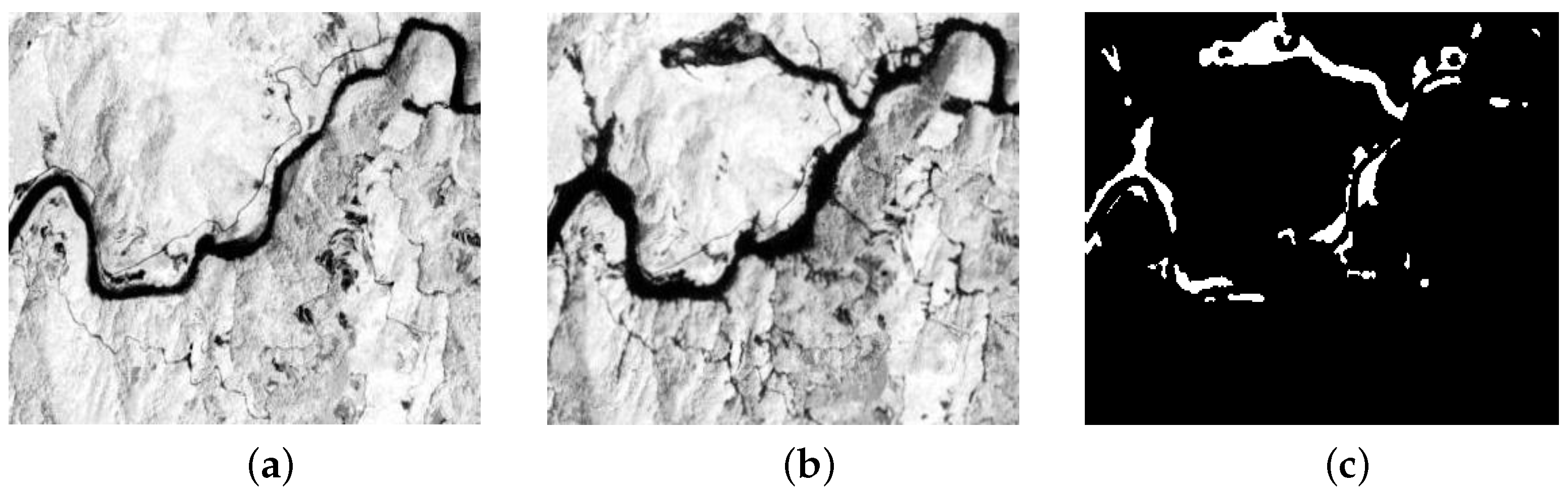
Figure 3.
Stone-Gate Reservoir data set: (a) SAR image 1; (b) SAR image 2; (c) ground-truth map.
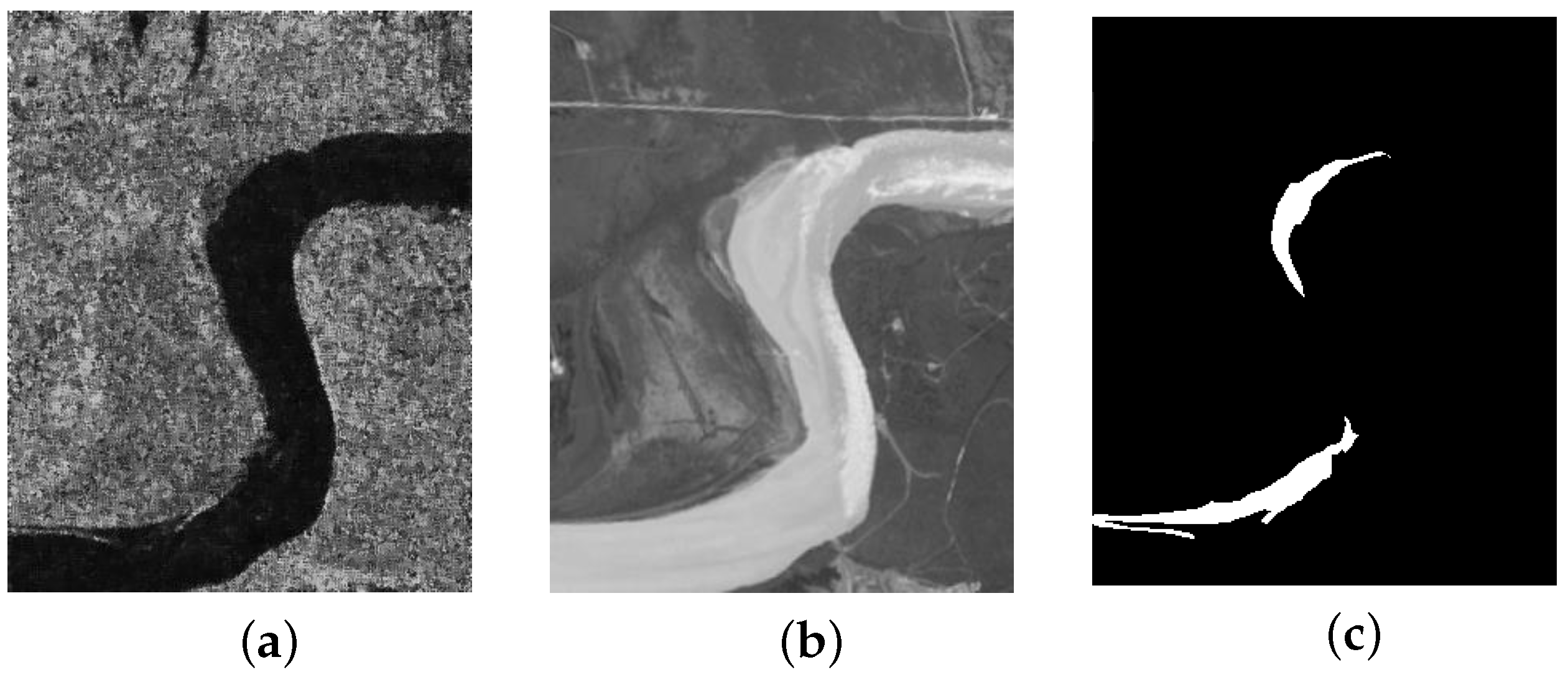
The second data set, known as the Yellow River data set, comprises a SAR image and an optical image, as shown in Figure 4. Both images have dimensions of with a spatial resolution of 8 m. This data set primarily highlights areas affected by floods.

Figure 4.
Yellow River data set: (a) SAR image; (b) optical image; (c) ground-truth map.
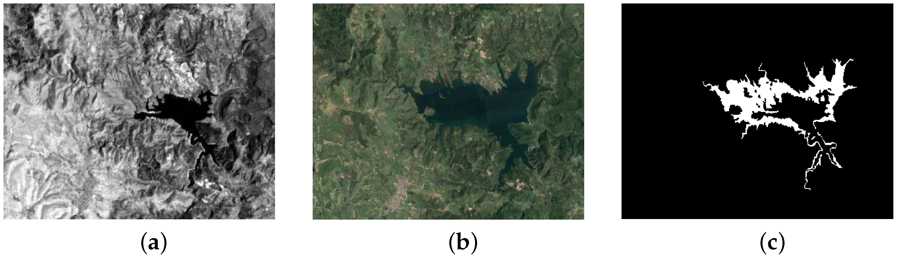
The third data set, known as the Sardinian data set, comprises a Landsat-5 TM image and an optical image, as shown in Figure 5. Both images have dimensions of and a resolution of 30 m. This data set documents the expansion of Lake Mulagea in Sardinia, Italy.

Figure 5.
Sardinia data set: (a) near-infrared band image; (b) optical image; (c) ground-truth map.
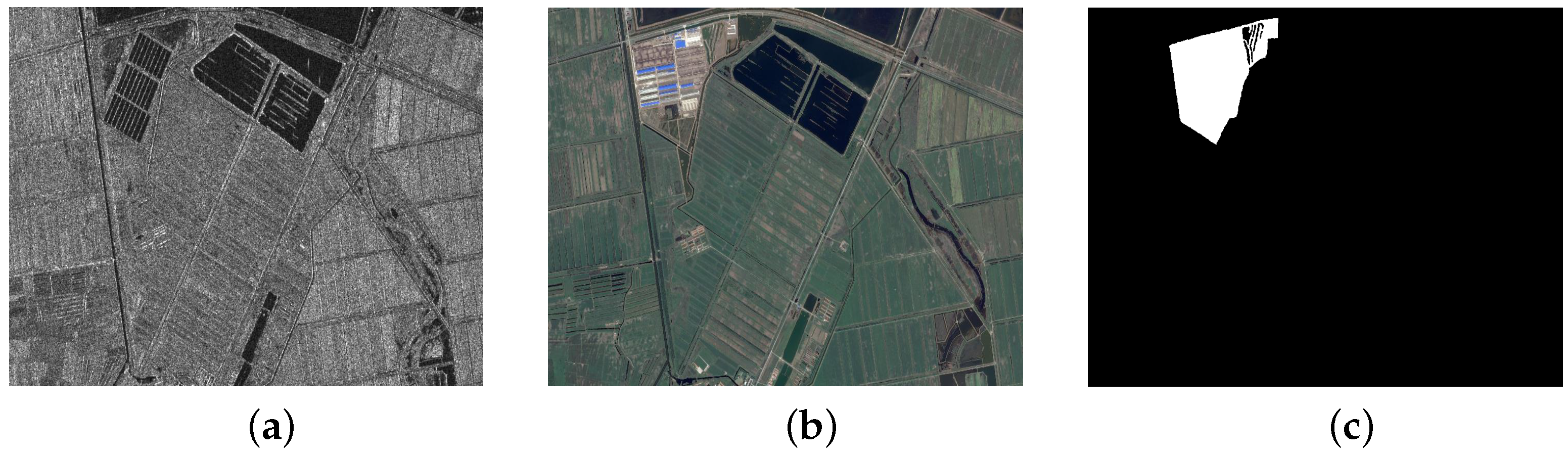
The fourth data set, named the Shuguang data set, comprises one SAR image and one optical image, as shown in Figure 6. Both images have dimensions of with a resolution of 8 m. This data set primarily illustrates instances where local residents have converted farmland to create additional space for buildings or other purposes.
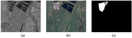
Figure 6.
Shuguang data set: (a) SAR image; (b) optical image; (c) ground-truth map.
(3) Parameter Setting Details for Experiments: The architecture of MJFM, as illustrated in Figure 2, represents individual pixels using small patches centered around them. These patches are input into each JFM. For small-scale patches, the patch size is set to , while for large-scale patches, it is . Each JFM’s encoder comprises four convolutional layers. The sizes of the first three convolutional layers are , with a stride of 1; a padding size of 1; and 32, 64, and 96 convolution kernels, respectively. The last convolutional layer’s kernel size is , with a stride of , no padding, and 128 convolution kernels. The output passes through a fully connected layer to yield the patch’s 16-lengthfeature vector. The decoder is symmetrical to the encoder structure and consists of four deconvolution layers and one fully connected layer. First, the 16-dimensional image patch features are input into a fully connected layer with a size of and activated by the LeakyReLU nonlinear function. Then, the 128-dimensional vector is input into the deconvolution layer for upsampling. The first deconvolution layer consists of 96 convolution kernels. The size of the convolution kernels is , the stride size is , and zero padding is not performed. The remaining three deconvolution layers are composed of 64, 32, and 3 convolution kernels, respectively. The convolution kernels’ size is , the stride size is 1, and the padding size is 1. Note that for each convolution layer and deconvolution layer, after convolution processing, the BatchNorm layer is used for normalization; then, the LeakyReLU function is used for nonlinear activation. The mapper consists of two fully connected layers with sizes of and , respectively. After each fully connected layer, a LeakyReLU nonlinear activation layer is added. MJFM’s learnable parameters are optimized using the backpropagation algorithm. Each JFM is trained using the Adam optimizer with a batch size of 128 examples, a learning rate of 0.0001, and exponential decay rates of 0.9 for the first moment estimate and 0.999 for the second moment estimate. The LeakyReLU activation function is utilized in each JFM layer. The feature vector’s Euclidean distance is computed and normalized to a range between 0 and 1, representing the normalized difference map.
In self-paced learning, selecting the appropriate step-speed parameter () can be challenging. As mentioned in [60], SPL computation can be streamlined by seeking a solution based on the number of training samples involved. We organize the losses of all training samples in ascending order to acquire , then designate the th loss value of as , represented as . After the self-paced learning phase, new samples are introduced, prompting a recalculation of . In subsequent experiments, we delve deeper into the influence of and on the model’s efficacy.
4.2. Test of Self-Paced Learning
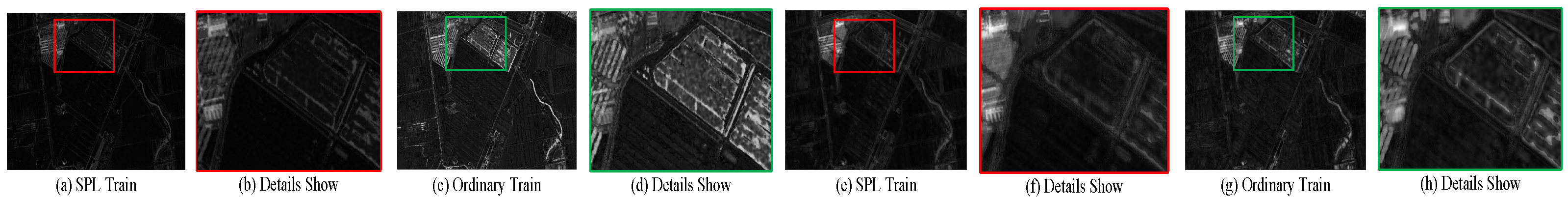
In order to verify the effect of self-paced learning on MJFM, we compare the difference map obtained by using the self-paced learning strategy to train MJFM with that obtained using an ordinary mode to train MJFM.
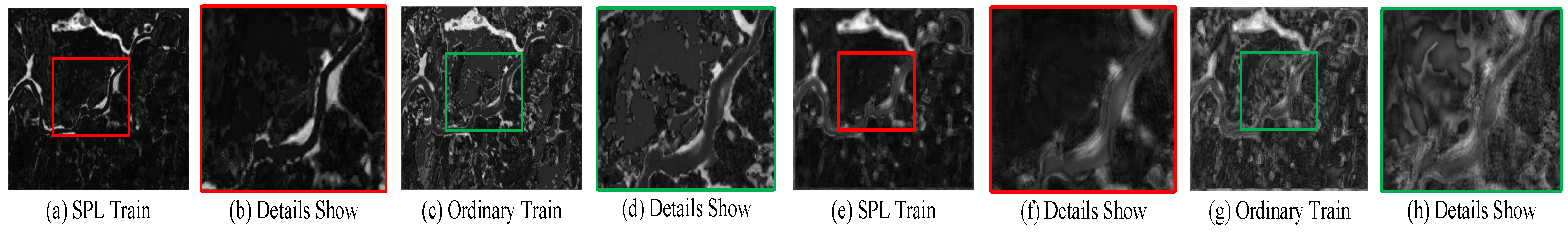
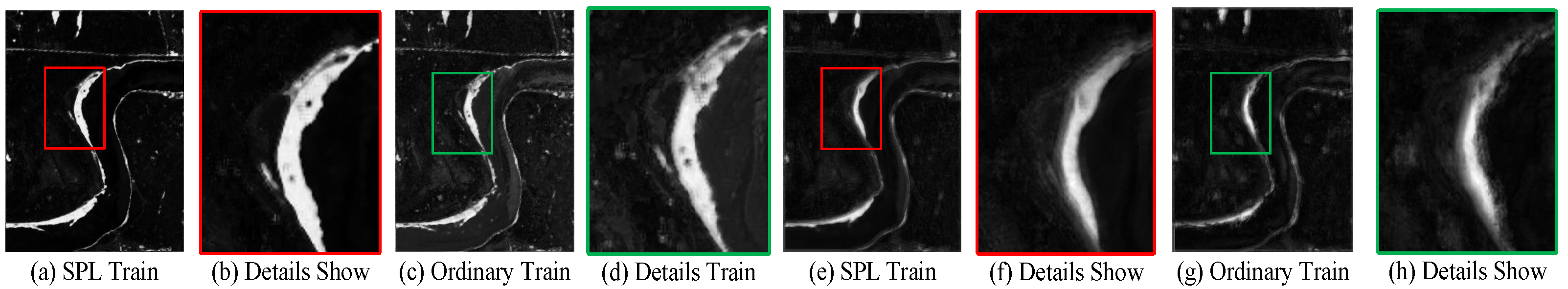
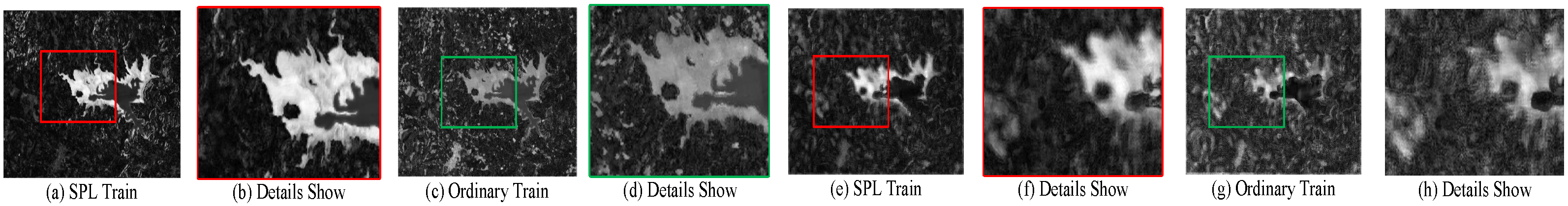
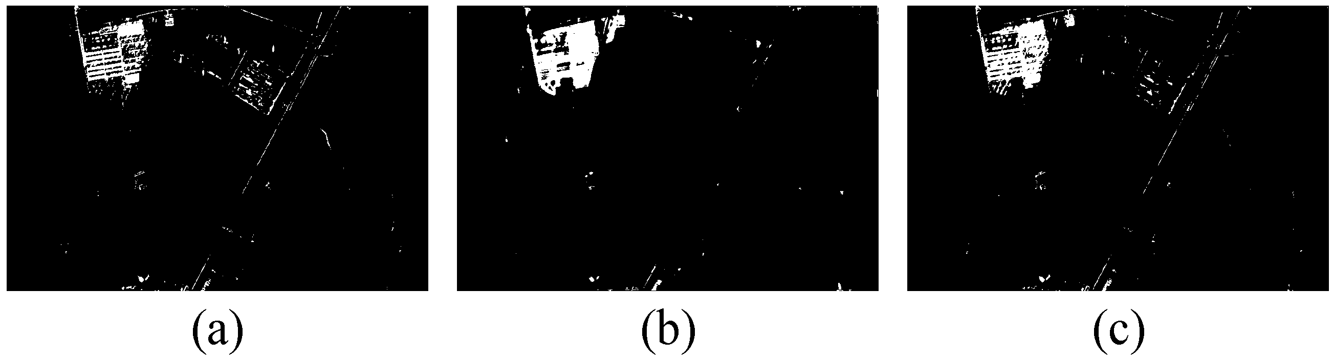
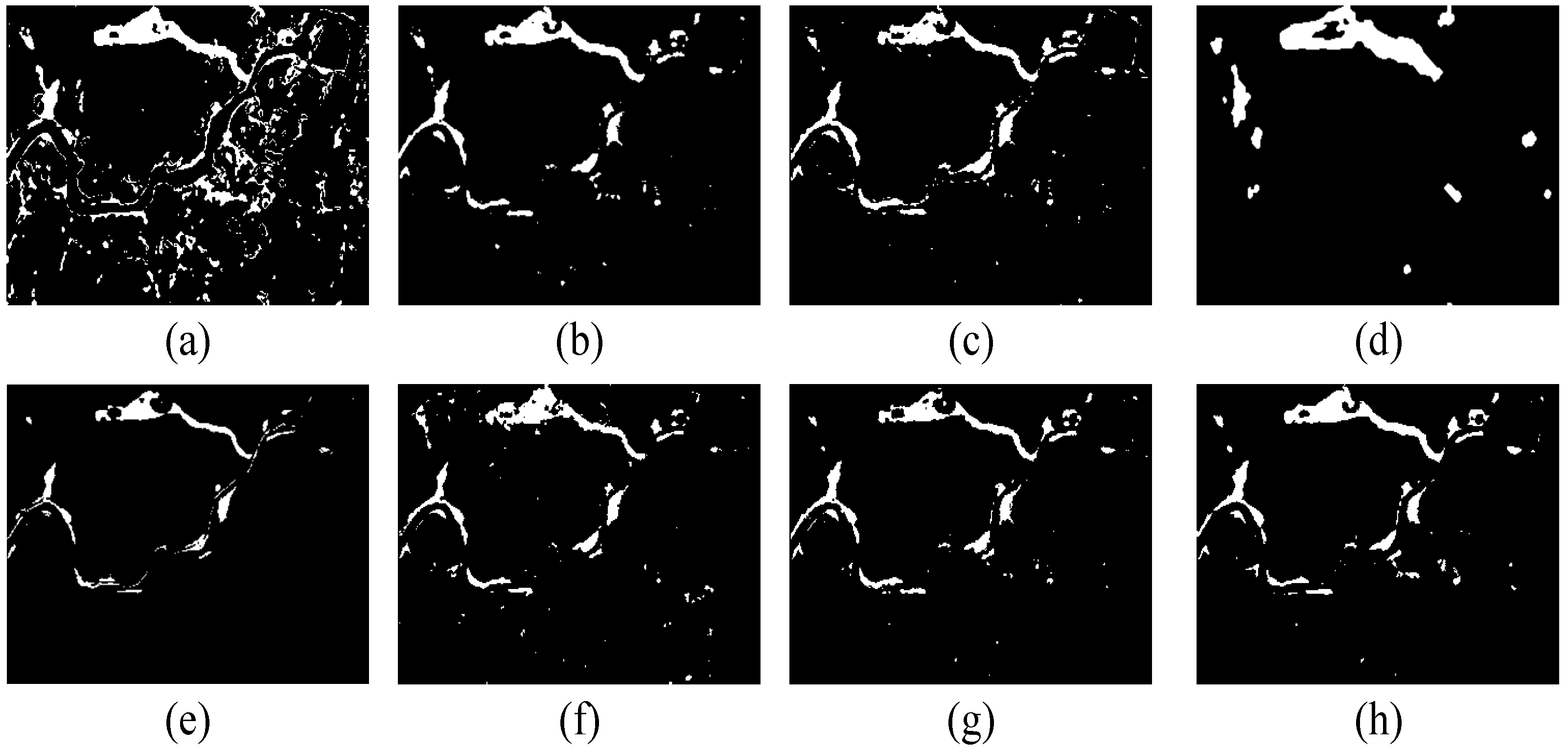
Figure 7, Figure 8, Figure 9 and Figure 10 record the difference maps generated by a JFM trained by a self-paced learning strategy and a JFM trained in normal mode on four data sets, where (a) and (c) are the difference maps obtained by small-scale JFMs, and (e) and (g) are the difference maps obtained by large-scale JFMs; (b), (d), (f), and (h) show the details of the difference maps. As previously analyzed, large-scale JFMs usually result in smoother difference maps but less detail retention, while small-scale JFMs result in higher detail retention but more abnormal noise points. In addition, it can be seen that after introducing the self-paced learning strategy into the JFM training process, the difference information of the generated difference map is more obvious. This is because the self-paced learning strategy focuses on low-loss samples, which are mainly distributed in the unchanged area in the remote sensing image. In the JFM training process, the high-loss samples in the changing area are usually weighted with a smaller weights relative to the loss, thereby inhibiting the model from learning the heterogeneous mapping relationship of this part of the sample. In the detailed display image, we can see that the JFM trained by the ordinary mode has more noise in the difference image. This is because the data of the changing region induce the non-uniform mapping on the JFM learning image, and this non-uniform mapping relationship causes the JFM to map the data of the unchanged region to the feature space with large differences, resulting in more noise in the unchanged region.
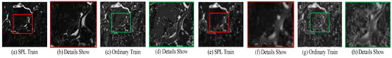
Figure 7.
Comparison of difference maps obtained by different training modes on the Stone-Gate data set.
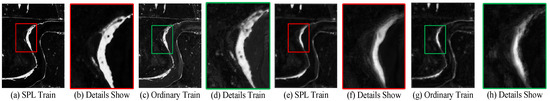
Figure 8.
Comparison of difference maps obtained by different training modes on the Yellow River data set.
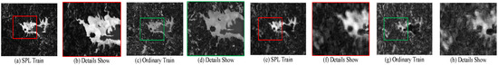
Figure 9.
Comparison of difference maps obtained by different training modes on the Sardinia data set.
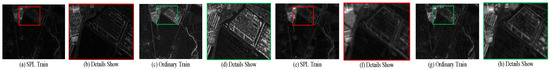
Figure 10.
Comparison of difference maps obtained by different training modes on the Shuguang data set.
4.3. Test of Self-Paced Learning Parameters
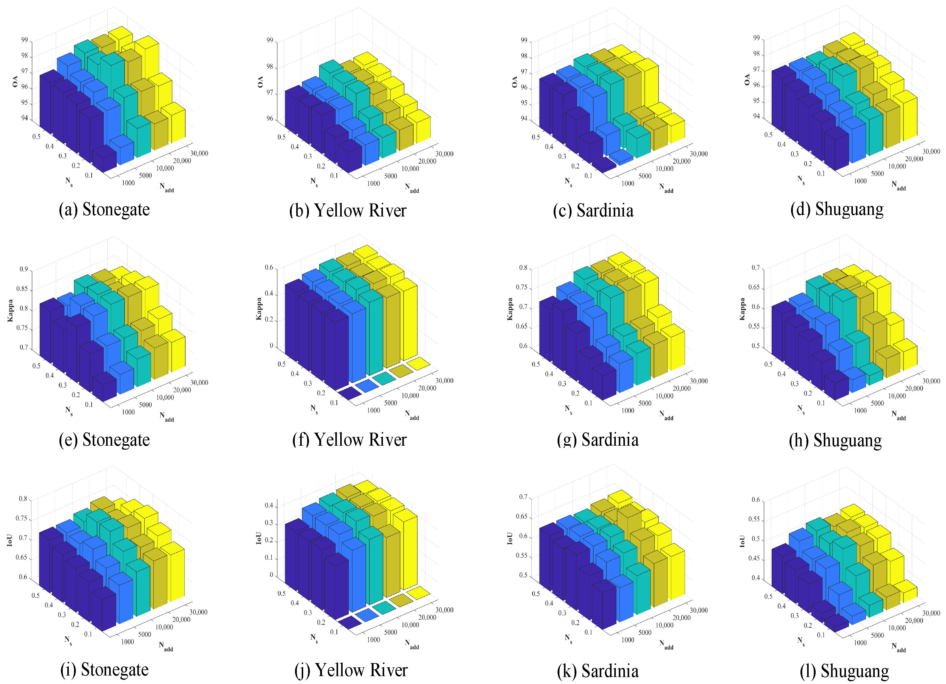
Selecting appropriate parameters has a significant impact on self-paced learning. In this paper, the SPL calculation is converted into a simpler calculation by searching for the solution of the number of samples involved in training. We conducted experiments on the initial and the sample increment parameter ().
In each iteration, the loss (L) of training-set samples is sorted in ascending order to obtain , and the th loss value of is chosen as the value of to create a training queue with non-zero weight values. After completing the inner loop of self-paced learning, training samples are appended to the training queue to increase the value (thus, in the subsequent iteration, the number of samples () in the self-paced learning training queue becomes ).
In the experiment, we initialize the training queue by selecting 10%, 20%, 30%, 40%, and 50% of the samples from the training set, then determine as . Subsequently, we gradually expand the training queue to sizes of 1000, 5000, 10,000, 20,000, and 30,000 until all training samples are included. Figure 11 illustrates the impact of and on the final change detection performance. It is observed that the framework demonstrates robustness to variations in and to a certain extent. Furthermore, it is noted that superior change detection outcomes are commonly attained when the initial training-queue size constitutes roughly 30% of the total training-set size, with around 10,000 samples added in each iteration. In addition, we do not recommend selecting a smaller initial training queue, which may lead to self-paced learning overfitting a single category of sample data, resulting in misclassification.
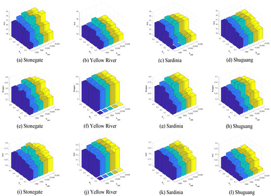
Figure 11.
Sensitivity analysis of self-paced learning parameters.
4.4. Test of Multi-Scale Learning
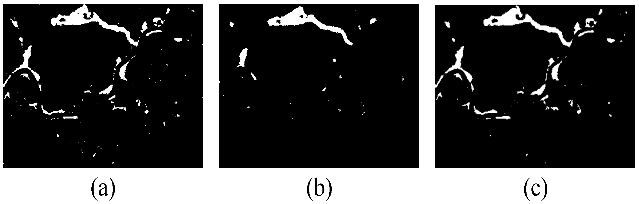
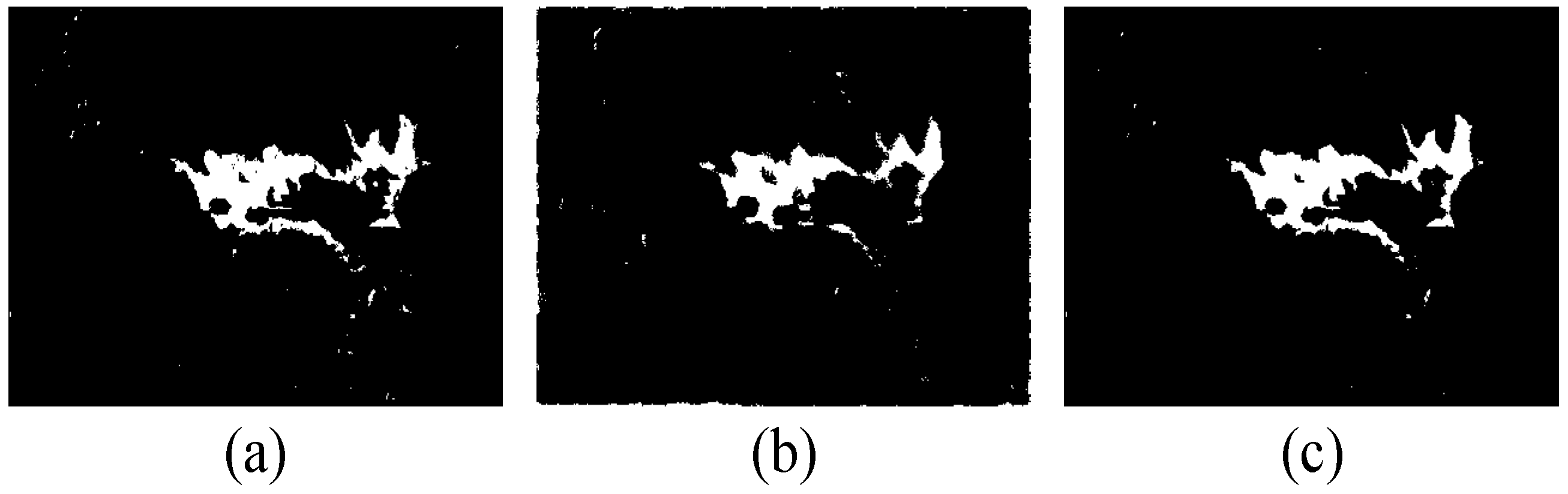
In this section, we test the impact of multi-scale learning on change detection performance. Specifically, for the multi-scale case, we use a pair of patches with sizes of and as input to MJFMand use MOPSO to post-process the difference map to obtain the change map. For the case of a single scale, we use and image patches as input to the JFM because in the case of a single scale, it is impossible to establish a multi-objective optimization problem for the difference map. Therefore, we use FCM to cluster the two difference maps to obtain the change map and record the relevant indicators of the change map obtained in these three cases. JFM-S means training the JFM with patches, and JFM-L means training the JFM with patches. Figure 12, Figure 13, Figure 14 and Figure 15 and Table 1 record the relevant results. It can be seen that in the case of a single scale, when the patch size is small, JFM-S detects more unchanged class pixels as changed classes. When the patch size is large, JFM-L detects more changed class pixels as unchanged classes. Multi-scale learning is complementary and greatly reduces the FP and FN indicators of change detection results. This is because multi-scale learning can make up for the lack of information in the case of a single scale and integrate the advantages of each scale, thereby providing richer information for change detection tasks and improving change detection performance.

Figure 12.
Change maps of the Stone-Gate data set. (a) JFM-S; (b) JFM-L; (c) SMJFM.
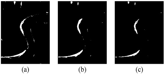
Figure 13.
Change maps of the Yellow River data set. (a) JFM-S; (b) JFM-L; (c) SMJFM.

Figure 14.
Change maps of the Sardinia data set. (a) JFM-S; (b) JFM-L; (c) SMJFM.

Figure 15.
Change maps of the Shuguang data set. (a) JFM-S; (b) JFM-L; (c) SMJFM.

Table 1.
Evaluation of multi-scale learning on four data sets.
4.5. Test of MOPSO
In order to evaluate the impact of MOPSO on change detection performance, we compare the change detection indices with and without MOPSO. In the first case, the robust evaluation threshold is set to 0.5. For the case without MOPSO, we perform an average weighted fusion of the two difference maps obtained by MJFM (i.e., ), then use FCM to classify the difference map to obtain the change map. The experimental results are shown in Table 2, where SMJFM represents our method, and CMJFM represents the method after removing MOPSO. It can be seen that in the absence of MOPSO, the FP index increases significantly, which means that there are more cases in which the unchanged class is misclassified into the changed class in the change map. This is because in SMJFM, we robustly evaluate the changed class pixels of the change map corresponding to multiple Pareto-optimal solutions, thus alleviating this situation. In addition, it can be seen that the use of MOPSO to post-process the difference map improves the OA and Kappa indices, which indicates that the introduction of MOPSO improves the processing performance from the difference map to the change map and can obtain a more accurate prediction change map closer to the original label map.
Table 2.
Evaluation of MOPSO on four data sets.
4.6. Test of Robust Evaluation of Change Map
In contrast to previous approaches such as thresholding or clustering methods for binarizing the difference map to obtain the change map, this paper leverages the information from the difference map at various scales. Initially, we present the Pareto frontier achieved by employing the multi-objective PSO algorithm, as depicted in Figure 16a–d. Subsequently, we assess the accuracy of the change-class labels on the four data sets using different thresholds and provide recommended threshold settings.
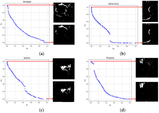
Figure 16.
The change maps obtained by weighing different objectives on the (a) Stone-Gate data set, (b) the Yellow River data set, (c) the Sardinia data set, and (d) the Shuguang data set.
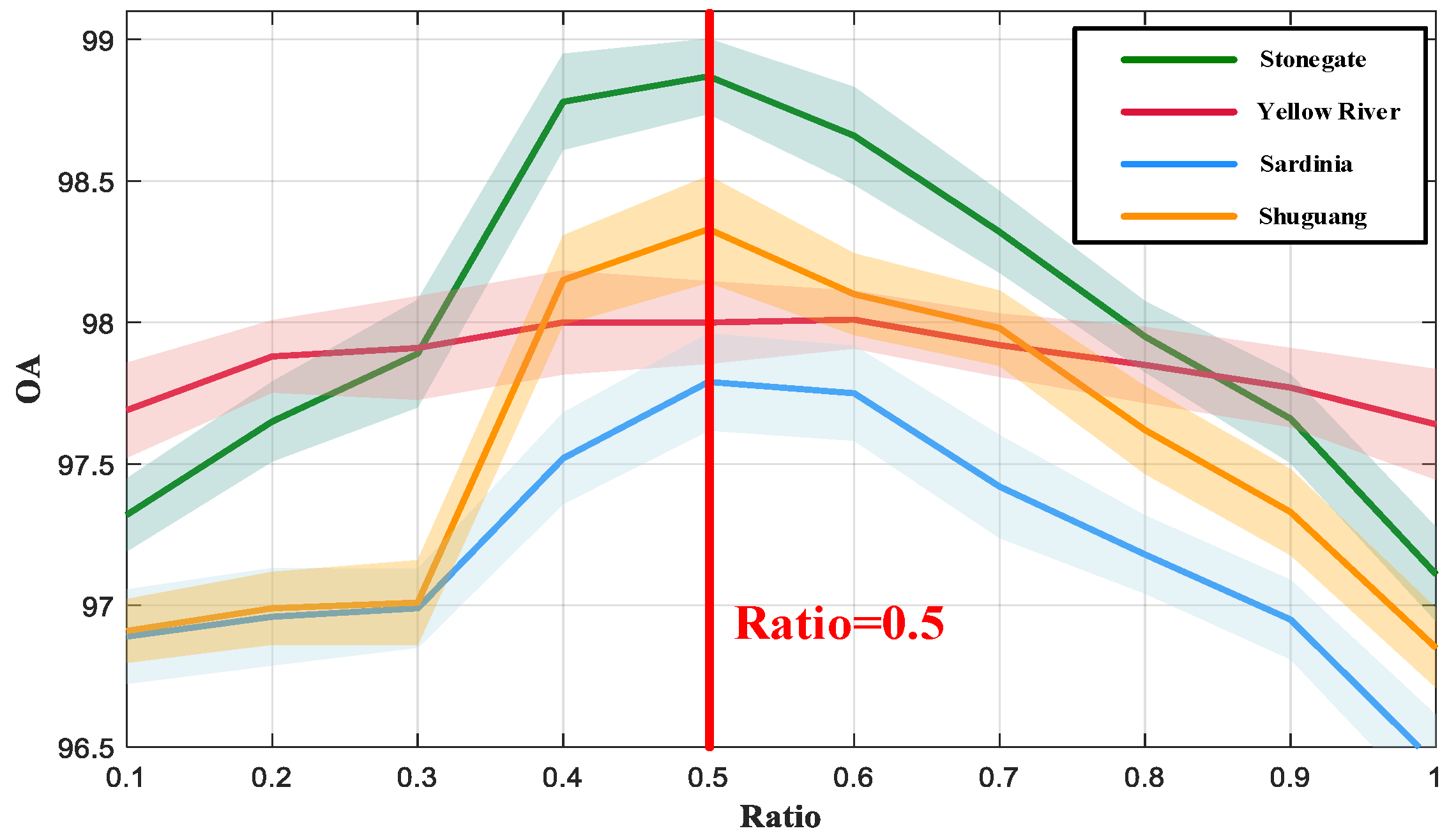
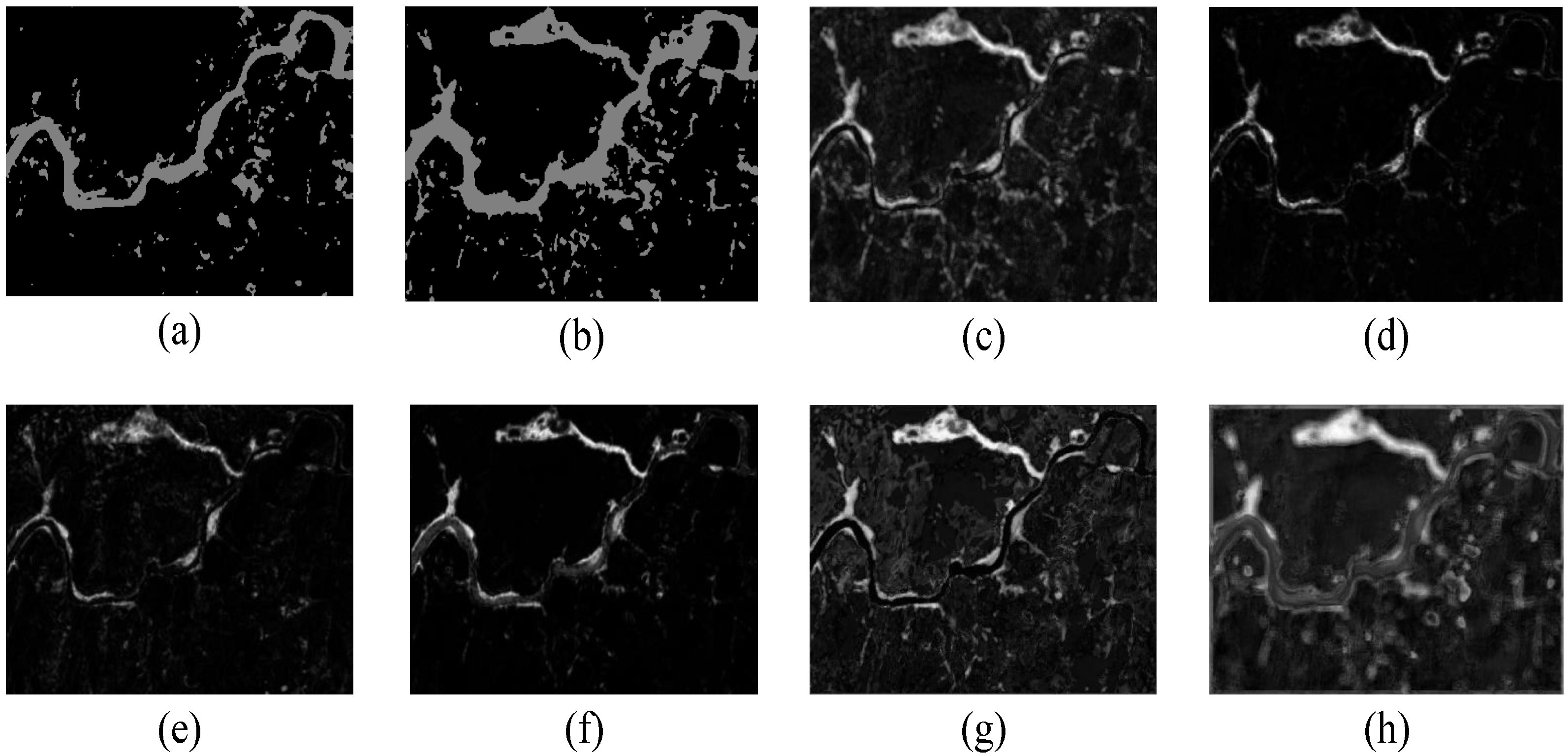
On the Pareto fronts of the four data sets, we show the change maps obtained by only considering noise suppression (i.e., clustering the difference maps obtained by the large-scale JFM) and only considering detail retention (i.e., clustering the difference maps obtained by the small-scale JFM). It can be clearly seen that in the case of only considering noise suppression, there are few isolated outliers on the generated change map, but the change map loses a lot of details, and the FN index on this change map will increase. If only the details are retained, there are many isolated outliers on the generated change map, and the FP index on this change map will increase. In order to make full use of the change information provided by the Pareto-optimal solutions, we use the change maps corresponding to all the Pareto-optimal solutions to robustly evaluate the change samples and set the threshold sequence to [0.1, 0.2, 0.3, 0.4, 0.5, 0.6, 0.7, 0.8, 0.9, 1.0]. In Figure 17, the change map’s OA index corresponding to different thresholds on four data sets is shown. It can be seen that when the robust evaluation threshold is near 0.5, better change detection results can usually be obtained. If the robust evaluation threshold is too large or too small, it will have a negative impact on the final detection results. This is because a smaller evaluation threshold cannot suppress the isolated abnormal samples on the change map, and a larger evaluation threshold will over-threshold the correct change samples on the change map, thereby reducing the overall accuracy.
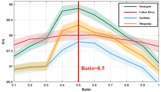
Figure 17.
Change maps obtained by weighing different objectives.
4.7. Test of Patch Size
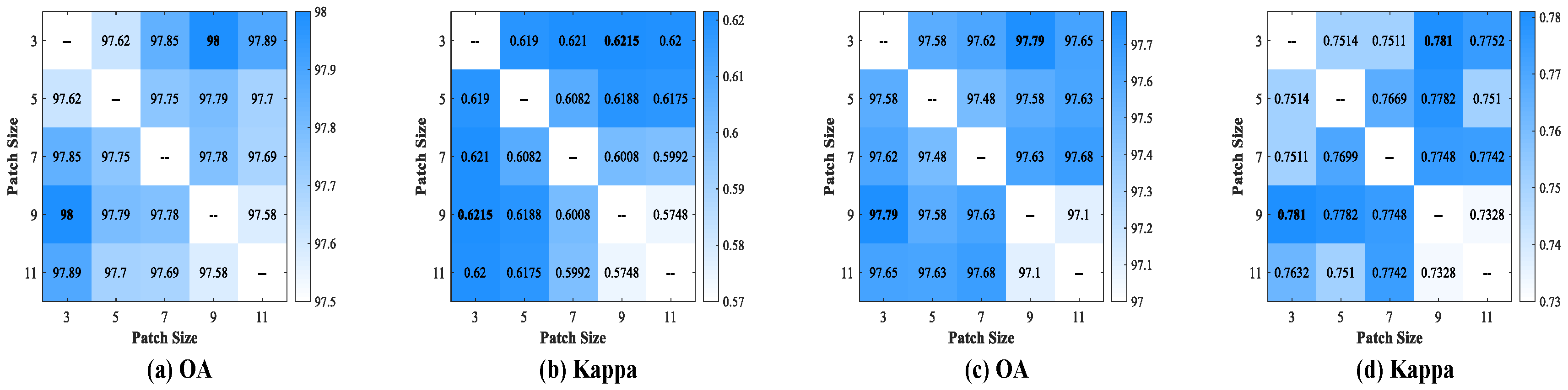
In order to compare the effects of different patch sizes on the change detection results, we change the patch size and record the final results while keeping other experimental settings unchanged. Specifically, we choose the Yellow River data set and the Sardinia data set, set different patch sizes, and calculate the OA index and Kappa index of the change map. Figure 18 is the experimental result. It can be seen that when the small-scale patch size is set to and the large-scale patch size is set to , the change detection result is the best. This may be because when the size of the small-scale patch is too large, fewer details of the change map are output by the JFM, and more errors are caused when change detection is performed on the ground–object boundary. When the large-scale patch is small, the model has difficulty in suppressing noise data and has low robustness to noise data. At the same time, it is not advisable to blindly increase the size of large-scale patches, which will make the difference map of the JFM output too vague, thus reducing the accuracy of change detection. Therefore, we recommend that the small-scale patch size be and the large-scale patch size be .
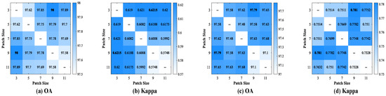
Figure 18.
The change detection results obtained under different patch-size settings. (a) OA of Yellow River data set; (b) Kappa of Yellow River data set; (c) OA of Sardinia data set; (d) Kappa of Sardinia data set.
4.8. Comparison of SMJFM against Other Methods
We compare our proposed framework with several existing methods, including PCC, MRF, CAN, SCCN, CACD, CDCG, and PMA.
4.8.1. Experiments on the Stone-Gate Data Set
This data set includes two panchromatic images. Despite the distinct characteristics of rivers and mountains, the presence of rainwater on mountaintops may lead to incorrect detection of unchanged areas as changed areas.
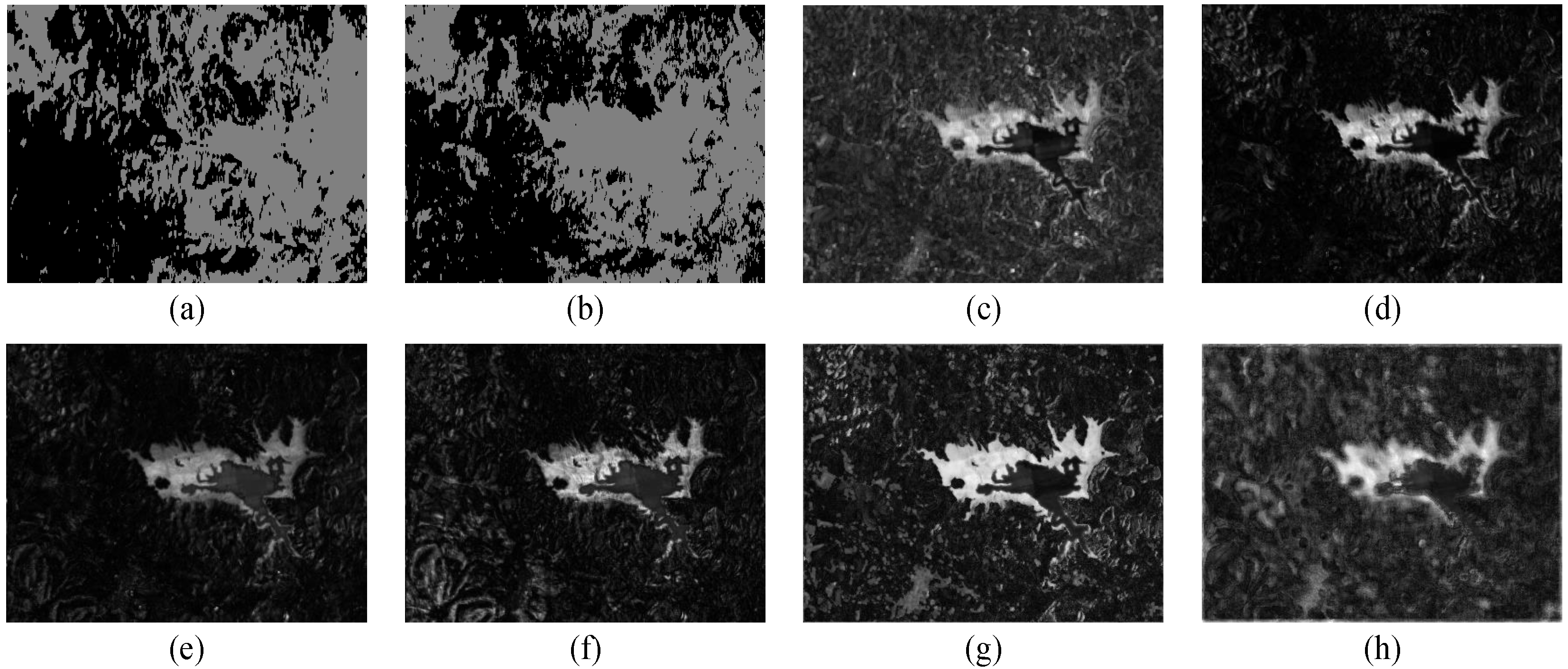
PCC utilizes FLICO to classify ground objects and subsequently detect change areas. Figure 19a,b display the classification results of PCC. Figure 19c–h depicts the difference maps obtained by SCCN, CACD, CGCD, PMA, the small-scale JFM (JFM-S), and the large-scale JFM (JFM-L), respectively. Notably, PCC, MRF, and CAN do not generate difference maps. Figure 20 displays the change maps obtained by all methods, while Table 3 presents the evaluation metrics for the change map acquired by each method. Compared to other methods, SMJFM does not incorporate any denoising algorithms, indicating that the complementary multi-scale information mechanism introduced by SMJFM inherently offers a denoising effect and demonstrates more promising detection performance.

Figure 19.
(a) Classification results of PCC algorithm for Figure 3a. (b) Classification results of PCC algorithm for Figure 3b. (c) Difference map generated by SCCN. (d) Difference map generated by CACD. (e) Difference map generated by CGCD. (f) Difference map generated by PMA. (g) Difference map generated by JFM-S. (h) Difference map generated by JFM-L.

Figure 20.
Change maps of Stone-Gate data set. (a) PCC; (b) SCCN; (c) CACD; (d) MRF; (e) CAN; (f) CGCD; (g) PMA; (h) SMJFM.
Table 3.
Evaluation on the Stone-Gate data set.
4.8.2. Experiments on the Yellow River Data Set
The features of the two images are simple; they just show land and river. The problem is in the significant speckle noise present in the SAR image. Figure 21a,b show the classification results of PCC. Figure 21c–h show the difference maps obtained by SCCN, CACD, CGCD, PMA, the small-scale JFM (JFM-S), and the large-scale JFM (JFM-L), respectively. Figure 22 is the change map obtained by all methods, and Table 4 is the index of the change map obtained by all methods. It can be seen that the change map obtained by SMJFM is the closest to the real label visually, the number of errors detected is smaller, and the overall accuracy is higher. In addition, it can be seen from Figure 21 that the comparison between the changed region and the unchanged region of the difference map obtained by SMJFM is more significant, which is due to the introduction of the self-paced learning training mechanism, while CACD only introduces common information into the feature vector, which leads to the autoencoder capturing the inconsistent mapping in the changed region during the learning process.
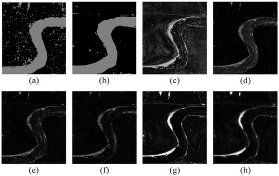
Figure 21.
(a) Classification results of PCC algorithm for Figure 4a. (b) Classification results of PCC algorithm for Figure 4b. (c) Difference map generated by SCCN. (d) Difference map generated by CACD. (e) Difference map generated by CGCD. (f) Difference map generated by PMA. (g) Difference map generated by JFM-S. (h) Difference map generated by JFM-L.
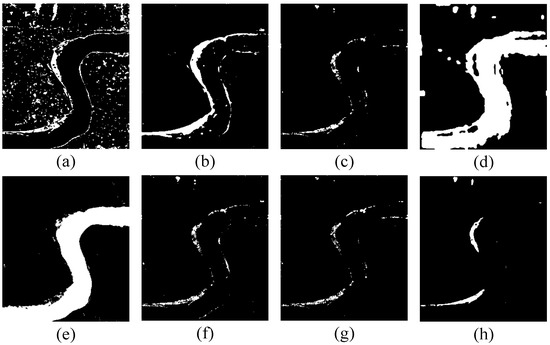
Figure 22.
Change maps of the Yellow River data set. (a) PCC; (b) SCCN; (c) CACD; (d) MRF; (e) CAN; (f) CGCD; (g) PMA; (h) SMJFM.
Table 4.
Evaluation on the Yellow River data set.
4.8.3. Experiments on the Sardinia Data Set
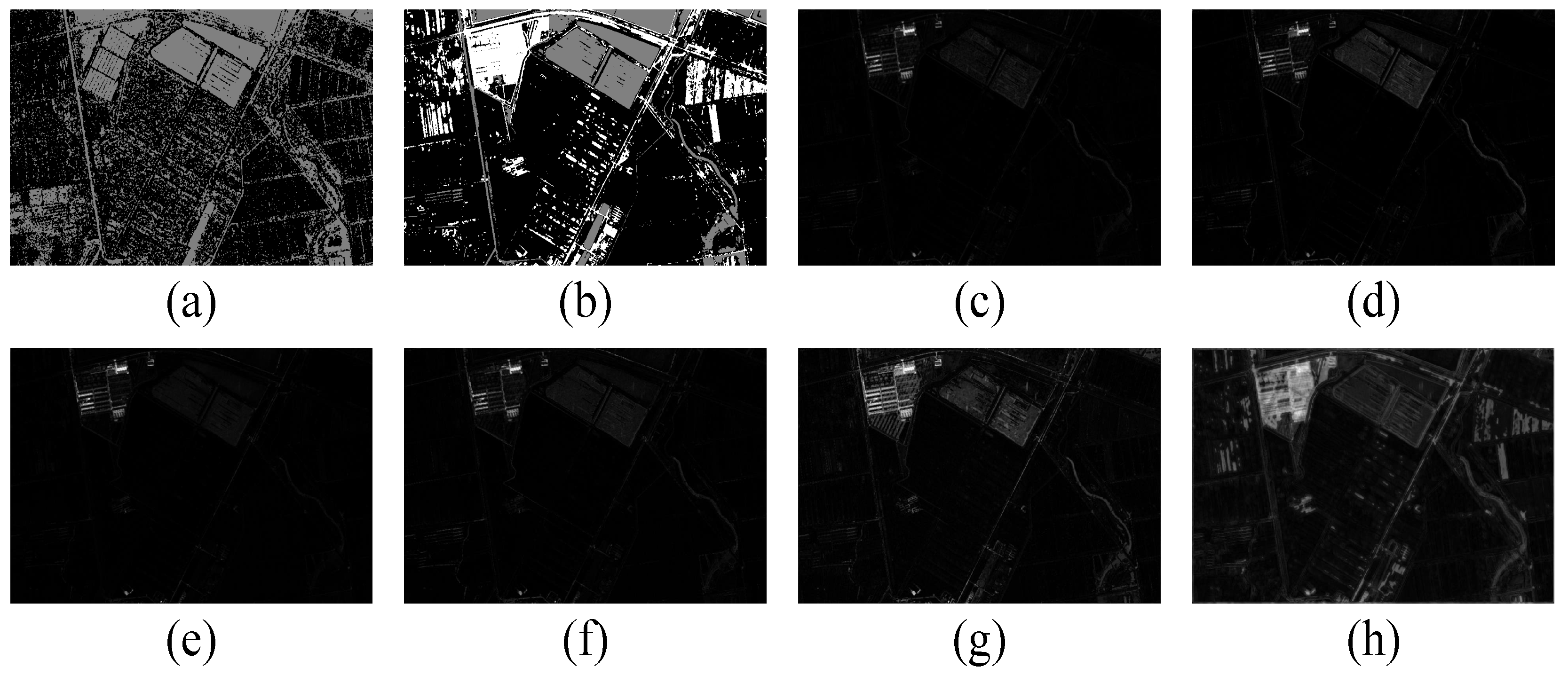
The heterogeneous images in this data set are mainly composed of mountains and water. The intricate texture features of the mountains pose the primary challenge in aligning the intricate elements of unchanged mountain features between the two images, while the second challenge involves identifying the characteristics of the water boundary. Figure 23a,b display the classification results of PCC, while Figure 23c–h depict the difference maps generated by SCCN, CACD, CGCD, PMA, the small-scale JFM (JFM-S), and the large-scale JFM (JFM-L), respectively. Figure 24 presents the change maps obtained by all methods, and Table 5 provides the evaluation indices of the change maps obtained by all methods. Due to the complex texture structure of the two images, the classification accuracy achieved by PCC is notably low. In contrast, SCCN, CACD, CGCD, and SMJFM map the two images to a more consistent potential space, thereby suppressing false positives in the unchanged region. Moreover, due to the substantial variation in the distribution of complex texture SAR image data and optical image data, the majority of pixels in the CAN image are misclassified.
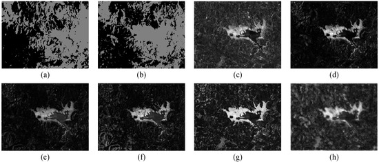
Figure 23.
(a) Classification results of PCC algorithm for Figure 5a. (b) Classification results of PCC algorithm for Figure 5b. (c) Difference map generated by SCCN. (d) Difference map generated by CACD. (e) Difference map generated by CGCD. (f) Difference map generated by PMA. (g) Difference map generated by JFM-S. (h) Difference map generated by JFM-L.

Figure 24.
Change maps of the Sardinia data set. (a) PCC; (b) SCCN; (c) CACD; (d) MRF; (e) CAN; (f) CGCD; (g) PMA; (h) SMJFM.
Table 5.
Evaluation on the Sardinia data set.
4.8.4. Experiments on the Shuguang Data Set
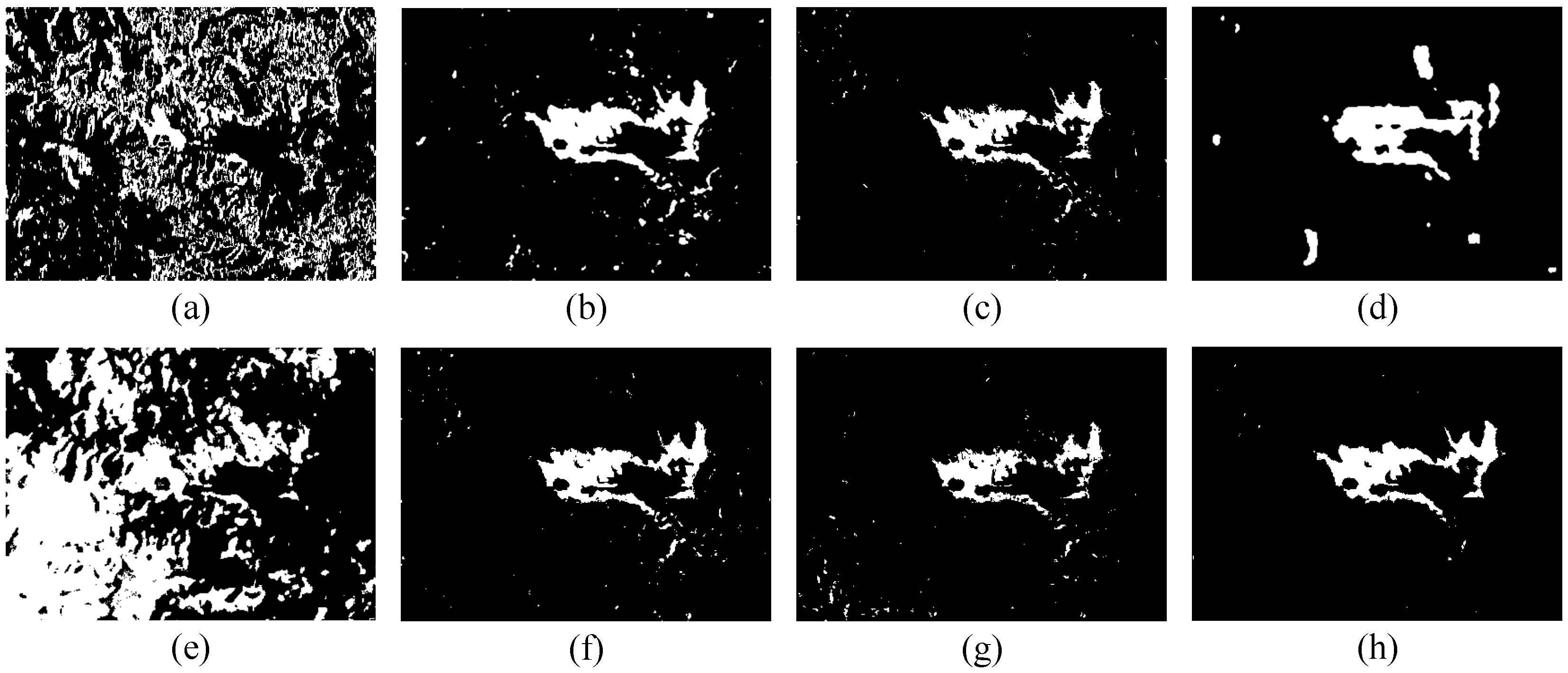
In comparison to the first three data sets, the fourth data set encompasses a broader array of ground items, including fields, buildings, and water areas, indicating the presence of numerous feature categories in these images. Consequently, the change detection task becomes increasingly challenging. In this data set, some attributes of the changed region closely resemble those of the unchanged region, leading to incorrect detection of these parts as unchanged. Distinguishing between these similar attributes poses a formidable challenge. Figure 25a,b illustrate the classification results of PCC, while Figure 25c–h display the difference diagrams generated by SCCN, CACD, CGCD, PMA, the small-scale JFM (JFM-S), and the large-scale JFM (JFM-L), respectively. Figure 26 presents the change maps obtained by all methods, and Table 6 provides the evaluation indices of the change maps obtained by all methods. From Figure 25, it can be observed that the difference maps generated by the CACD, SCCN, CGCD, and PMA methods are not satisfactory, as the feature difference in the change area is minimal, leading to an increase in the FN index in the change map. Meanwhile, although the difference map generated by the small-scale JFM is subpar, the difference map obtained by the large-scale JFM effectively highlights the change area. Thanks to the robust evaluation mechanism of Pareto-optimal solutions, an excellent change map is ultimately achieved.

Figure 25.
(a) Classification results of PCC algorithm for Figure 6a. (b) Classification results of PCC algorithm for Figure 6b. (c) Difference map generated by SCCN. (d) Difference map generated by CACD. (e) Difference map generated by CGCD. (f) Difference map generated by PMA. (g) Difference map generated by JFM-S. (h) Difference map generated by JFM-L.
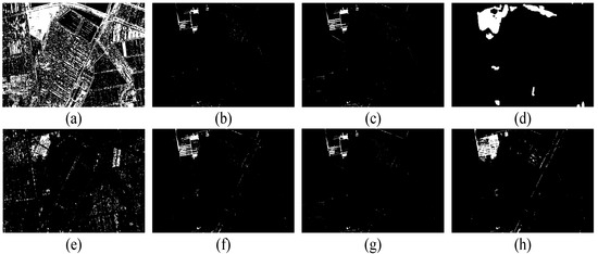
Figure 26.
Change maps of the Shuguang data set. (a) PCC; (b) SCCN; (c) CACD; (d) MRF; (e) CAN; (f) CDCG; (g) PMA; (h) SMJFM.
Table 6.
Evaluation on the Shuguang data set.
5. Conclusions
This paper proposes an unsupervised method for detecting changes in heterogeneous images. The method consists of several key components. First, it introduces a multi-scale joint feature mapper (MJFM) based on an autoencoder architecture to effectively map heterogeneous data into comparable feature spaces. Secondly, it incorporates a self-paced learning training strategy to guide the MJFM in capturing the mapping relationship of unchanged regions while avoiding overfitting to changed regions. Finally, it balances noise suppression and detail retention objectives and utilizes a robust evaluation method to obtain a high-precision binary change image. The proposed method demonstrates resilience to noise in remote sensing images and effectively mitigates change detection errors stemming from complex ground-object information, ensuring its applicability across diverse scenarios. In addition, since the proposed framework does not require supervised information, this framework can handle more diverse remote sensing image (underwater remote sensing images, hyperspectral remote sensing images, etc.) change detection problems.
Author Contributions
Conceptualization, Y.W., R.Y. and M.G.; software, K.D., Q.S. and H.L.; formal analysis, K.D.; investigation, Y.W. and K.D.; resources, Y.W. and K.D.; data curation, Y.W. and K.D.; writing—original draft preparation, Y.W., K.D. and Q.S.; writing—review and editing, R.Y. and M.G.; visualization, K.D. and Q.S.; supervision, Y.W. and H.L.; project administration, R.Y. and M.G.; funding acquisition, H.L. and M.G. All authors have read and agreed to the published version of the manuscript.
Funding
This work was supported in part by the National Natural Science Foundation of China under Grant 62036006 and in part by the Fundamental Research Funds for the Central Universities.
Data Availability Statement
The original contributions presented in the study are included in the article, further inquiries can be directed to the corresponding author.
Conflicts of Interest
The authors declare no conflicts of interest.
References
- Shi, J.; Wu, T.; Qin, A.K.; Lei, Y.; Joen, G. Self-Guided Autoencoders for Unsupervised Change Detection in Heterogeneous Remote Sensing Images. IEEE Trans. Artif. Intell. 2024. [Google Scholar] [CrossRef]
- Gong, M.; Zhao, J.; Liu, J.; Miao, Q.; Jiao, L. Change detection in synthetic aperture radar images based on deep neural networks. IEEE Trans. Neural Netw. Learn. Syst. 2015, 27, 125–138. [Google Scholar] [CrossRef] [PubMed]
- Wen, Y.; Ma, X.; Zhang, X.; Pun, M.O. GCD-DDPM: A generative change detection model based on difference-feature guided DDPM. IEEE Trans. Geosci. Remote Sens. 2024. [Google Scholar] [CrossRef]
- Ji, Y.; Sun, W.; Wang, Y.; Lv, Z.; Yang, G.; Zhan, Y.; Li, C. Domain Adaptive and Interactive Differential Attention Network for Remote Sensing Image Change Detection. IEEE Trans. Geosci. Remote Sens. 2024. [Google Scholar] [CrossRef]
- Jin, S.; Yang, L.; Zhu, Z.; Homer, C. A land cover change detection and classification protocol for updating Alaska NLCD 2001 to 2011. Remote Sens. Environ. 2017, 195, 44–55. [Google Scholar] [CrossRef]
- Yin, H.; Pflugmacher, D.; Li, A.; Li, Z.; Hostert, P. Land use and land cover change in Inner Mongolia-understanding the effects of China’s re-vegetation programs. Remote Sens. Environ. 2018, 204, 918–930. [Google Scholar] [CrossRef]
- Leichtle, T.; Geiß, C.; Wurm, M.; Lakes, T.; Taubenböck, H. Unsupervised change detection in VHR remote sensing imagery–an object-based clustering approach in a dynamic urban environment. Int. J. Appl. Earth Obs. Geoinf. 2017, 54, 15–27. [Google Scholar] [CrossRef]
- Leichtle, T.; Geiß, C.; Lakes, T.; Taubenböck, H. Class imbalance in unsupervised change detection–a diagnostic analysis from urban remote sensing. Int. J. Appl. Earth Obs. Geoinf. 2017, 60, 83–98. [Google Scholar] [CrossRef]
- Luo, H.; Liu, C.; Wu, C.; Guo, X. Urban change detection based on Dempster–Shafer theory for multitemporal very high-resolution imagery. Remote Sens. 2018, 10, 980. [Google Scholar] [CrossRef]
- Wang, S.; Ma, Q.; Ding, H.; Liang, H. Detection of urban expansion and land surface temperature change using multi-temporal landsat images. Resour. Conserv. Recycl. 2018, 128, 526–534. [Google Scholar] [CrossRef]
- Liu, J.; Gong, M.; Qin, K.; Zhang, P. A deep convolutional coupling network for change detection based on heterogeneous optical and radar images. IEEE Trans. Neural Netw. Learn. Syst. 2016, 29, 545–559. [Google Scholar] [CrossRef] [PubMed]
- Gong, M.; Zhang, P.; Su, L.; Liu, J. Coupled dictionary learning for change detection from multisource data. IEEE Trans. Geosci. Remote Sens. 2016, 54, 7077–7091. [Google Scholar] [CrossRef]
- Li, M.; Li, M.; Zhang, P.; Wu, Y.; Song, W.; An, L. SAR image change detection using PCANet guided by saliency detection. IEEE Geosci. Remote Sens. Lett. 2018, 16, 402–406. [Google Scholar] [CrossRef]
- Zhao, M.; Ling, Q.; Li, F. An iterative feedback-based change detection algorithm for flood mapping in SAR images. IEEE Geosci. Remote Sens. Lett. 2018, 16, 231–235. [Google Scholar] [CrossRef]
- Zheng, Y.; Jiao, L.; Liu, H.; Zhang, X.; Hou, B.; Wang, S. Unsupervised saliency-guided SAR image change detection. Pattern Recognit. 2017, 61, 309–326. [Google Scholar] [CrossRef]
- De, S.; Pirrone, D.; Bovolo, F.; Bruzzone, L.; Bhattacharya, A. A novel change detection framework based on deep learning for the analysis of multi-temporal polarimetric SAR images. In Proceedings of the 2017 IEEE International Geoscience and Remote Sensing Symposium (IGARSS), Fort Worth, TX, USA, 23–28 July 2017; pp. 5193–5196. [Google Scholar]
- Hou, B.; Liu, Q.; Wang, H.; Wang, Y. From W-Net to CDGAN: Bitemporal change detection via deep learning techniques. IEEE Trans. Geosci. Remote Sens. 2019, 58, 1790–1802. [Google Scholar] [CrossRef]
- Lu, X.; Yuan, Y.; Zheng, X. Joint dictionary learning for multispectral change detection. IEEE Trans. Cybern. 2016, 47, 884–897. [Google Scholar] [CrossRef] [PubMed]
- Xiang, Y.; Wang, F.; Wan, L.; Jiao, N.; You, H. OS-flow: A robust algorithm for dense optical and SAR image registration. IEEE Trans. Geosci. Remote Sens. 2019, 57, 6335–6354. [Google Scholar] [CrossRef]
- Li, W.; Li, Y.; Chan, J.C.W. Thick cloud removal with optical and SAR imagery via convolutional-mapping-deconvolutional network. IEEE Trans. Geosci. Remote Sens. 2019, 58, 2865–2879. [Google Scholar] [CrossRef]
- Xiang, Y.; Tao, R.; Wan, L.; Wang, F.; You, H. OS-PC: Combining feature representation and 3-D phase correlation for subpixel optical and SAR image registration. IEEE Trans. Geosci. Remote Sens. 2020, 58, 6451–6466. [Google Scholar] [CrossRef]
- Coello, C.A.C. Evolutionary Algorithms for Solving Multi-Objective Problems; Springer: New York, NY, USA, 2007. [Google Scholar]
- Fonseca, C.M.; Fleming, P.J. An overview of evolutionary algorithms in multiobjective optimization. Evol. Comput. 1995, 3, 1–16. [Google Scholar] [CrossRef]
- Bengio, Y.; Louradour, J.; Collobert, R.; Weston, J. Curriculum learning. In Proceedings of the 26th Annual International Conference on Machine Learning, Montreal, QC, Canada, 14–18 June 2009; pp. 41–48. [Google Scholar]
- Volpi, M.; Tuia, D.; Bovolo, F.; Kanevski, M.; Bruzzone, L. Supervised change detection in VHR images using contextual information and support vector machines. Int. J. Appl. Earth Obs. Geoinf. 2013, 20, 77–85. [Google Scholar] [CrossRef]
- Qin, Y.; Niu, Z.; Chen, F.; Li, B.; Ban, Y. Object-based land cover change detection for cross-sensor images. Int. J. Remote Sens. 2013, 34, 6723–6737. [Google Scholar] [CrossRef]
- Mercier, G.; Moser, G.; Serpico, S.B. Conditional copulas for change detection in heterogeneous remote sensing images. IEEE Trans. Geosci. Remote Sens. 2008, 46, 1428–1441. [Google Scholar] [CrossRef]
- Volpi, M.; Camps-Valls, G.; Tuia, D. Spectral alignment of multi-temporal cross-sensor images with automated kernel canonical correlation analysis. ISPRS J. Photogramm. Remote Sens. 2015, 107, 50–63. [Google Scholar] [CrossRef]
- Prendes, J.; Chabert, M.; Pascal, F.; Giros, A.; Tourneret, J.Y. Change detection for optical and radar images using a Bayesian nonparametric model coupled with a Markov random field. In Proceedings of the 2015 IEEE International Conference on Acoustics, Speech and Signal Processing (ICASSP), South Brisbane, QLD, Australia, 19–24 April 2015; pp. 1513–1517. [Google Scholar]
- Yuan, F.; Sawaya, K.E.; Loeffelholz, B.C.; Bauer, M.E. Land cover classification and change analysis of the Twin Cities (Minnesota) Metropolitan Area by multitemporal Landsat remote sensing. Remote Sens. Environ. 2005, 98, 317–328. [Google Scholar] [CrossRef]
- Wu, Y.; Bai, Z.; Miao, Q.; Ma, W.; Yang, Y.; Gong, M. A classified adversarial network for multi-spectral remote sensing image change detection. Remote Sens. 2020, 12, 2098. [Google Scholar] [CrossRef]
- Lv, Z.; Huang, H.; Sun, W.; Jia, M.; Benediktsson, J.A.; Chen, F. Iterative training sample augmentation for enhancing land cover change detection performance with deep learning neural network. IEEE Trans. Neural Netw. Learn. Syst. 2023. [Google Scholar] [CrossRef] [PubMed]
- Li, H.; Gong, M.; Zhang, M.; Wu, Y. Spatially self-paced convolutional networks for change detection in heterogeneous images. IEEE J. Sel. Top. Appl. Earth Obs. Remote Sens. 2021, 14, 4966–4979. [Google Scholar] [CrossRef]
- Xu, C.; Liu, B.; He, Z. A New Method for False Alarm Suppression in Heterogeneous Change Detection. Remote Sens. 2023, 15, 1745. [Google Scholar] [CrossRef]
- Touati, R.; Mignotte, M.; Dahmane, M. A new change detector in heterogeneous remote sensing imagery. In Proceedings of the 2017 Seventh International Conference on Image Processing Theory, Tools and Applications (IPTA), Montreal, QC, Canada, 28 November–1 December 2017; pp. 1–6. [Google Scholar]
- Gong, M.; Niu, X.; Zhan, T.; Zhang, M. A coupling translation network for change detection in heterogeneous images. Int. J. Remote Sens. 2019, 40, 3647–3672. [Google Scholar] [CrossRef]
- Touati, R.; Mignotte, M.; Dahmane, M. Change detection in heterogeneous remote sensing images based on an imaging modality-invariant MDS representation. In Proceedings of the 2018 25th IEEE International Conference on Image Processing (ICIP), Athens, Greece, 7–10 October 2018; pp. 3998–4002. [Google Scholar]
- Liu, Z.; Li, G.; Mercier, G.; He, Y.; Pan, Q. Change detection in heterogenous remote sensing images via homogeneous pixel transformation. IEEE Trans. Image Process. 2017, 27, 1822–1834. [Google Scholar] [CrossRef] [PubMed]
- Chen, H.; Wu, C.; Du, B.; Zhang, L.; Wang, L. Change detection in multisource VHR images via deep siamese convolutional multiple-layers recurrent neural network. IEEE Trans. Geosci. Remote Sens. 2019, 58, 2848–2864. [Google Scholar] [CrossRef]
- Zhang, P.; Gong, M.; Su, L.; Liu, J.; Li, Z. Change detection based on deep feature representation and mapping transformation for multi-spatial-resolution remote sensing images. ISPRS J. Photogramm. Remote Sens. 2016, 116, 24–41. [Google Scholar] [CrossRef]
- Wu, Y.; Li, J.; Yuan, Y.; Qin, A.K.; Miao, Q.G.; Gong, M.G. Commonality autoencoder: Learning common features for change detection from heterogeneous images. IEEE Trans. Neural Netw. Learn. Syst. 2021, 33, 4257–4270. [Google Scholar] [CrossRef]
- Xing, Y.; Zhang, Q.; Ran, L.; Zhang, X.; Yin, H.; Zhang, Y. Progressive Modality-Alignment for Unsupervised Heterogeneous Change Detection. IEEE Trans. Geosci. Remote Sens. 2023. [Google Scholar] [CrossRef]
- Touati, R.; Mignotte, M.; Dahmane, M. Multimodal change detection in remote sensing images using an unsupervised pixel pairwise-based Markov random field model. IEEE Trans. Image Process. 2019, 29, 757–767. [Google Scholar] [CrossRef] [PubMed]
- Li, H.; Gong, M.; Wang, C.; Miao, Q. Pareto self-paced learning based on differential evolution. IEEE Trans. Cybern. 2019, 51, 4187–4200. [Google Scholar] [CrossRef]
- Li, H.; Wan, F.; Gong, M.; Qin, A.; Wu, Y.; Xing, L. Privacy-enhanced multitasking particle swarm optimization based on homomorphic encryption. IEEE Trans. Evol. Comput. 2023. [Google Scholar] [CrossRef]
- Lyu, K.; Li, H.; Gong, M.; Xing, L.; Qin, A. Surrogate-Assisted Evolutionary Multiobjective Neural Architecture Search based on Transfer Stacking and Knowledge Distillation. IEEE Trans. Evol. Comput. 2023. [Google Scholar] [CrossRef]
- Gong, M.; Li, H.; Luo, E.; Liu, J.; Liu, J. A multiobjective cooperative coevolutionary algorithm for hyperspectral sparse unmixing. IEEE Trans. Evol. Comput. 2016, 21, 234–248. [Google Scholar] [CrossRef]
- Li, H.; Gong, M.; Wang, Q.; Liu, J.; Su, L. A multiobjective fuzzy clustering method for change detection in SAR images. Appl. Soft Comput. 2016, 46, 767–777. [Google Scholar] [CrossRef]
- Gong, M.; Li, H.; Meng, D.; Miao, Q.; Liu, J. Decomposition-based evolutionary multiobjective optimization to self-paced learning. IEEE Trans. Evol. Comput. 2018, 23, 288–302. [Google Scholar] [CrossRef]
- Kumar, M.P.; Turki, H.; Preston, D.; Koller, D. Learning specific-class segmentation from diverse data. In Proceedings of the 2011 International Conference on Computer Vision, Barcelona, Spain, 6–13 November 2011; pp. 1800–1807. [Google Scholar]
- Lee, Y.J.; Grauman, K. Learning the easy things first: Self-paced visual category discovery. In Proceedings of the CVPR 2011, Colorado Springs, CO, USA, 20–25 June 2011; pp. 1721–1728. [Google Scholar]
- Tang, K.; Ramanathan, V.; Fei-Fei, L.; Koller, D. Shifting weights: Adapting object detectors from image to video. Adv. Neural Inf. Process. Syst. 2012, 25. [Google Scholar]
- Supancic, J.S.; Ramanan, D. Self-paced learning for long-term tracking. In Proceedings of the IEEE Conference on Computer Vision and Pattern Recognition, Portland, OR, USA, 23–28 June 2013; pp. 2379–2386. [Google Scholar]
- Jiang, L.; Meng, D.; Mitamura, T.; Hauptmann, A.G. Easy samples first: Self-paced reranking for zero-example multimedia search. In Proceedings of the 22nd ACM International Conference on Multimedia, Orlando, FL, USA, 3–7 November 2014; pp. 547–556. [Google Scholar]
- Jiang, L.; Meng, D.; Yu, S.I.; Lan, Z.; Shan, S.; Hauptmann, A. Self-paced learning with diversity. Adv. Neural Inf. Process. Syst. 2014, 27. [Google Scholar]
- Jiang, L.; Meng, D.; Zhao, Q.; Shan, S.; Hauptmann, A. Self-paced curriculum learning. In Proceedings of the AAAI Conference on Artificial Intelligence, Austin, TX, USA, 25–30 January 2015; Volume 29. [Google Scholar]
- Zhao, Q.; Meng, D.; Jiang, L.; Xie, Q.; Xu, Z.; Hauptmann, A. Self-paced learning for matrix factorization. In Proceedings of the AAAI Conference on Artificial Intelligence, Austin, TX, USA, 25–30 January 2015; Volume 29. [Google Scholar]
- Zhang, D.; Meng, D.; Li, C.; Jiang, L.; Zhao, Q.; Han, J. A self-paced multiple-instance learning framework for co-saliency detection. In Proceedings of the 2015 IEEE International Conference on Computer Vision, Santiago, Chile, 7–13 December 2015; pp. 594–602. [Google Scholar]
- Kumar, M.; Packer, B.; Koller, D. Self-paced learning for latent variable models. Adv. Neural Inf. Process. Syst. 2010, 23. [Google Scholar]
- Li, H.; Gong, M.; Meng, D.; Miao, Q. Multi-objective self-paced learning. In Proceedings of the AAAI Conference on Artificial Intelligence, Phoenix, AZ, USA, 12–17 February 2016; Volume 30. [Google Scholar]


Disclaimer/Publisher’s Note: The statements, opinions and data contained in all publications are solely those of the individual author(s) and contributor(s) and not of MDPI and/or the editor(s). MDPI and/or the editor(s) disclaim responsibility for any injury to people or property resulting from any ideas, methods, instructions or products referred to in the content. |
© 2024 by the authors. Licensee MDPI, Basel, Switzerland. This article is an open access article distributed under the terms and conditions of the Creative Commons Attribution (CC BY) license (https://creativecommons.org/licenses/by/4.0/).