Disentangling the Influential Factors Driving NPP Decrease in Shandong Province: An Analysis from Time Series Evaluation Using MODIS and CASA Model

Abstract

Net Primary Productivity (NPP) is a critical metric for assessing terrestrial carbon sequestration and ecosystem health. While advancements in NPP modeling have enabled estimation at various scales, hidden anomalies within NPP time series necessitate further investigation to understand the driving forces. This study focuses on Shandong Province, China, generating a high-resolution (250 m) monthly NPP product for 2000–2019 using the Carnegie–Ames–Stanford Approach (CASA) model, integrated with satellite remote sensing and ground observations. We employed the Seasonal Mann–Kendall (SMK) Test and the Breaks For Additive Season and Trend (BFAST) algorithm to differentiate between gradual declines and abrupt losses, respectively. Beyond analyzing land use and land cover (LULC) transitions, we utilized Random Forest models to elucidate the influence of environmental factors on NPP changes. The findings revealed a significant overall increase in annual NPP across the study area, with a moderate average of 503.45 gC/(m²·a) during 2000–2019. Although 69.67% of the total area displayed a substantial monotonic increase, 3.89% of the area experienced abrupt NPP losses, and 8.43% exhibited gradual declines. Our analysis identified LULC transitions, primarily driven by urban expansion, as being responsible for 55% of the abrupt loss areas and 33% of the gradual decline areas. Random Forest models effectively explained the remaining areas, revealing that the magnitude of abrupt losses and the intensity of gradual declines were driven by a complex interplay of factors. These factors varied across vegetation types and change types, with explanatory variables related to vegetation status and climatic factors—particularly precipitation—having the most prominent influence on NPP changes. The study suggests that intensified land use and extreme climatic events have led to NPP diminishment in Shandong Province. Nevertheless, the prominent positive vegetation growth trends observed in some areas highlight the potential for NPP enhancement and carbon sequestration through targeted management strategies.

1. Introduction

Vegetation serves as the primary component of terrestrial ecosystems. Enhancing the carbon sequestration capacity of vegetation has emerged as a pivotal strategy to mitigate the impacts of climate change [1,2,3]. Net Primary Productivity (NPP) is a vital metric used to measure the carbon sequestration capacity of terrestrial vegetation. It refers to the residual amount of organic dry matter produced by green plants through photosynthesis per unit time and area after accounting for autotrophic respiration [4,5,6]. NPP determines the quantity of newly produced organic resources available to all other organisms within an ecosystem. As such, it is a crucial metric for understanding the health and fundamental function of terrestrial ecosystems, as well as for evaluating the impacts of environmental changes or management practices on these ecosystems [7,8]. Accurate estimation of regional vegetation NPP and analysis of its spatial and temporal distribution characteristics and driving factors can facilitate a deeper understanding of the functional stability, health status, and change trends of ecosystems. This, in turn, can provide a scientific basis for the protection and restoration of ecosystems.

Previous research has established a variety of models for estimating vegetation productivity at regional and global scales. These models can be broadly categorized into three types: climate-based productivity models, ecological and physiological process models, and Light Use Efficiency (LUE) models [9,10,11]. Climate productivity models, including the Miami model and the Thornthwaite Memorial model, are empirical models based on the relationship between vegetation productivity and climate factors [12,13]. These models primarily consider climate factors such as temperature and precipitation but overlook the effects of solar radiation and vegetation type on NPP. Ecological and physiological process models, such as the Terrestrial Ecosystem Model (TEM) and the Biome Biogeochemical Cycle (Biome-BGC) model, simulate vegetation NPP based on ecological and biogeochemical process theories. These models consider a large number of influencing factors and exhibit high modeling accuracy. However, they are complex and have limited spatial generalization ability [14]. LUE models are designed to simulate the absorption and conversion ability of plants to solar radiation under varying climatic conditions [15,16,17]. Commonly used models include the Carnegie–Ames–Stanford Approach (CASA) model [18,19,20,21,22], the EC-LUE model [23], the GLO-PEM [24], and the MuSyQ-NPP model [25]. As a representative of LUE models, the CASA model is distinguished for its robust process-based framework, efficient data integration, and continuous refinement. Its versatility and adaptability have been demonstrated through successful applications across various land cover types and climatic conditions worldwide. Moreover, its performance has been rigorously assessed through extensive validation against ground-based measurements and flux tower data, affirming its reliability and accuracy in productivity estimation.

Given the significance of NPP, it is crucial to monitor its changes, determine the influential factors, and decipher the underlying mechanisms [26]. Previous studies have analyzed the spatiotemporal dynamics of NPP from time series data obtained from stationary flux towers’ in situ measurements or from model estimates that span scales from the local to the global [27,28]. The dynamics of NPP can be characterized from various perspectives, including phenology changes, trend direction, rate of change, and interannual variability. With the development of NPP estimation models and the continuous improvement of remote sensing vegetation feature products, wall-to-wall NPP monitoring and analysis can now be conducted reliably on a monthly basis [29]. This advancement allows for more precise attention to be paid to the abnormal signals hidden in the NPP time series (e.g., abrupt changes) beyond the gradual trend. These signals may have been overlooked due to insufficient temporal resolution or may have been incorrectly attributed to gradual trends. Abnormal changes in NPP can serve as an indicator that a particular ecosystem is undergoing significant alterations. These alterations could potentially lead to substantial shifts in the ecosystem’s structure and functions and, in extreme cases, even trigger ecosystem collapse. Therefore, understanding abnormal changes in NPP is critical for monitoring ecosystem health and predicting ecosystem changes.

It is widely recognized that vegetation NPP is influenced by a myriad of factors [26,30]. These include climate variables (e.g., warming, drought, CO₂ concentration, and heatwaves), biogeochemical factors (e.g., nutrient availability, hydrology, and soil properties), disturbance agents (e.g., wildfires, insect outbreaks, harvest, and land use and land cover (LULC) transition), and inherent ecosystem characteristics. Understanding the specific drivers and their interactions is useful for predicting how NPP might respond to changing environmental conditions [31,32,33]. Previous studies have established robust linkages between gradual NPP trends (either decline or rise) and environmental drivers (climatic factors, ecosystem structures, biodiversity, etc.) [34,35,36]. Few studies have quantitatively delineated the relationships between abrupt NPP anomalies and the aforementioned environmental factors. Furthermore, such relationships may vary significantly across different ecosystems, but this has not yet received enough research attention. Ongoing climate change and increasing anthropogenic pressure may trigger unexpected shifts in disturbance regimes and alter ecosystem vulnerability. This can be directly reflected via abrupt loss in the NPP time series. Therefore, it is urgent to form an in-depth understanding of these interactions. This knowledge is crucial for supporting decision-making processes related to regional ecosystem protection and sustainable resource management.

Shandong Province, located in Eastern China, is subject to a unique combination of pressures, including a rapidly growing economy, a dense population, and a diverse range of ecosystems. Its rapid social and economic development has given rise to a host of issues, such as environmental pollution, rapid changes in LULC, high resource consumption, and degraded ecosystem services. Despite recent studies indicating an overall increasing trend in the NPP of Shandong Province, there are areas of NPP decrease. These areas, especially where there is a gradual decline or abrupt loss, should be given particular attention but have instead been largely overlooked. Given the crucial role Shandong Province will play in meeting China’s carbon neutrality goals [37], it is important to accurately estimate and monitor the dynamics of vegetation NPP. The information on NPP decrease obtained from this study will contribute to informing sustainable agricultural practices, optimizing forestry management, and guiding the development of renewable energy sources.

With this study, we aimed to monitor NPP changes and reveal the driving forces in Shandong Province for the period from 2000 to 2019. Our specific objectives were (1) to generate wall-to-wall NPP time series datasets based on the CASA model with adequate spatiotemporal granularity for capturing change signals; (2) to distinguish and characterize gradual and abrupt changes in NPP trends through time series analysis; and (3) to determine the driving effects of environmental factors on the gradually declining trend and abrupt loss intensity of NPP. To address these objectives, we designed a per-pixel time series analysis framework to detect abnormal decreases from monthly NPP evaluations. We quantitatively analyzed the driving factors leading to the NPP decrease through land use and land cover transition and machine learning models. Our research is anticipated to contribute to filling the knowledge gap concerning the mechanisms underlying ecosystem productivity responses to environmental changes in North China.

2. Materials and Methods

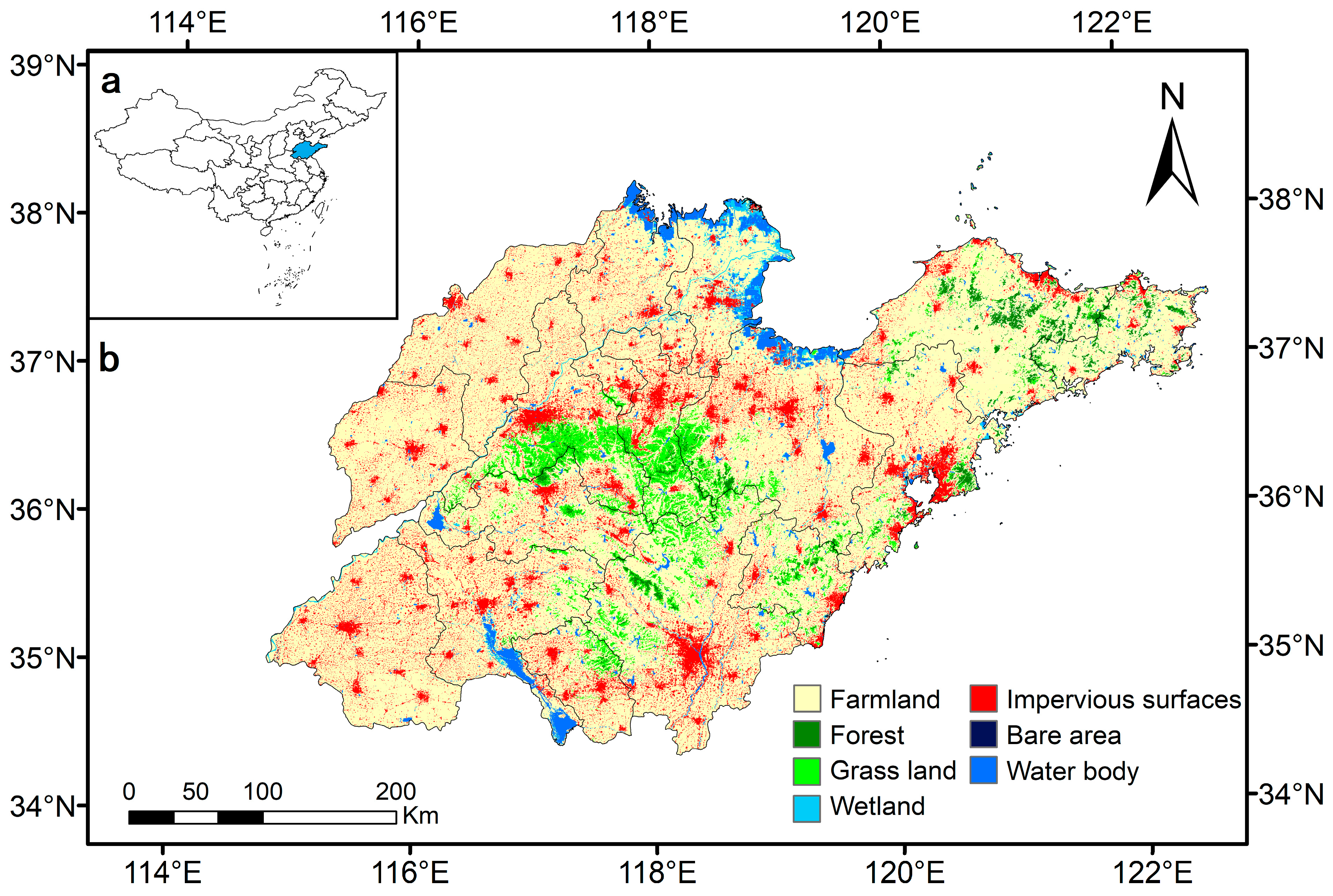
2.1. Study Area

The study area encompasses 1.58 × 10⁵ km² of Shandong Province, situated along the eastern coastline of China (Figure 1). The province resides within the warm-temperate monsoon zone, characterized by pronounced seasonal variations. Summers are typically hot and humid, with average temperatures ranging from 24 °C to 27 °C and monsoon rains invigorating the landscape. Winters are relatively cool and dry, with temperatures dipping to between 3 °C and −3 °C. Precipitation varies across the province, with coastal areas receiving approximately 600 mm annually, while the mountainous western regions experience up to 1000 mm. The topography of Shandong Province presents diverse landscapes. The fertile and expansive eastern plains rise gently toward the central region, punctuated by ancient volcanic remnants such as Mount Tai. In the west, the landscape transitions into dramatic, rugged mountains carved by the Yellow River, its majestic course weaving through gorges and alluvial plains. This varied terrain plays a vital role in shaping local microclimates and supporting diverse ecosystems. Mountains and hills account for 33% of the total area. The dominant land cover type is farmland, which occupies about 76% of the land area [38], where signature crops such as corn, wheat, soybeans, and peanuts are cultivated. The forest types in Shandong Province are diverse, including coniferous forests, broad-leaved forests, and shrub forests. Coniferous forests, primarily composed of pines and firs, are mainly distributed in the western mountainous areas. Broad-leaved forests, with oaks and maples as the main species, are primarily found in the eastern plains. Shrublands are mainly distributed along the edges of mountains and hilly areas.

2.2. Datasets

To estimate monthly NPP via the CASA model, validate reliability, and analyze the driving forces, we utilized a series of datasets (

Table 1. Sources and details of meteorological and remote sensing data.

Dataset	Data Name	Data Source *	Period	Temporal Resolution	Spatial Resolution
Vegetation index	MOD13Q1	NASA	2000–2019	16-day	250 m
Land cover	GLC_FCS30	AIRI	2000–2019	5-year	30 m
MODIS NPP	MOD17A3HGF Version 6.1	NASA	2000–2019	Yearly	500 m
GLASS NPP	NPP_MODIS_500m_V60	UMD	2000–2019	8-day	500 m
Meteorological observation	High spatial resolution monthly meteorological dataset for China	TPDC	2000–2019	Monthly	1 km
Solar duration	SURF_CLI_CHN_MUL_DAY V3.0	CMDC	2000–2019	Daily	-
Elevation	ASTER GDEMv3	NESSDC	-	-	30 m
Road net	gROADSv1	SEDAC	2013	-	-
Nighttime light	Harmonized Global NTL Dataset	Scientific Data	2019	Annual	1 km
Population data	LandScan Global Population	LGPD	2019	Annual	1 km

Note *: NASA—National Aeronautics and Space Administration; AIRI—Aerospace Information Research Center in Chinese Academy of Sciences; UMD—University of Maryland; TPDC—National Tibetan Plateau Data Center; CMDC—China Meteorological Data Service Centre; NESSDC—National Earth System Science Data Center; SEDAC—Socioeconomic Data and Applications Center; LGPD—LandScan Global Population Database.

). These included remote sensing vegetation index products, land cover maps, NPP products, meteorological observations of weather variables, solar radiation, and the Digital Elevation Model (DEM). To ensure spatial alignment across all datasets used in this study, we adopted the combination of the WGS-84 ellipsoid and UTM Zone 50N projection as the geographic reference system. Beyond two NPP products, all spatial datasets were either acquired or processed to a spatial resolution of 250 m. Those datasets were all highly credible products that have been publicly released on national-level data platforms, and most of them have undergone peer review in high-level academic journals. A comprehensive description of these datasets, including source, spatial, and temporal resolutions, among other details, can be found in Table 1.

The vegetation index (VI) data adopted here were from the MOD13Q1 V6 product (Greenbelt, MD, USA), obtained from the NASA Moderate Resolution Imaging Spectroradiometer (MODIS) website (see https://ladsweb.modaps.eosdis.nasa.gov, accessed on 26 May 2024). This product can provide two types of VIs, the Normalized Difference Vegetation Index (NDVI) and the Enhanced Vegetation Index (EVI), at 250 m every 16 days. To obtain monthly VI data that are consistent with the temporal resolution of the meteorological data, we converted this 16-day VI product into a monthly product by using the mean value of VIs that fell in the same month. The GLC_FCS30 product (Beijing, China) can provide global land cover mapping with a fine classification system at five-year intervals from 1985 to 2020. The refined classification system is well aligned with the NPP modeling requirement for ecosystem types [39]. To ensure the land cover maps had a consistent spatial resolution of 250 m, we applied an 8 × 8 moving window analysis to spatially aggregate the majority of land cover types within the window, first to 240 m, and then applied the nearest neighbor resampling to produce maps at 250 m. Here, we processed five periods of GLC_FCS30 product from 2000 to 2020 as the input for subsequent NPP estimation modeling procedures.

Two widely recognized NPP products in the academic community, such as the MOD17A3HGF (Greenbelt, MD, USA) and GLASS (Beijing, China), were used to validate the reliability of our estimation. They both quantified NPP at 500 m but differed in temporal resolution. We generated a cumulative composite of yearly GLASS NPP from an 8-day interval to match the MOD17A3HGF product. We preserved the original 500 m resolution to minimize data loss due to the resampling process.

The gridded meteorological data at a spatial resolution of 1 km × 1 km were acquired from the National Tibetan Plateau Data Centre [40], including mean monthly temperature (MMT), mean monthly precipitation (MMP), potential evapotranspiration (PET), and actual evapotranspiration (AET). Here, we resampled the product into 250 m using a bilinear interpolation approach. The terrestrial solar radiation was calculated using the empirical relationship between atmospheric external radiation and sunshine percentage as proposed by [41]. The atmospheric external radiation, a function of geographic latitude, solar declination, hour angle, solar constant, and the average relative distance between the sun and the earth, was easily calculated based on the geographic conditions of a given location. The primary external input data, daily sunshine duration observations, were obtained from the China Meteorological Data Service Center. We obtained data from 62 stations covering Shandong Province and the surrounding areas. We applied an IDW interpolation method to generate daily sunshine duration at 250 m grain size. The detailed calculation of solar radiation can be found in Supplementary Table S1 [42].

To represent human activities, we used the distance to the nearest road [43], Nighttime Light (NTL) [44] intensity, and population [45] as surrogate variables. We used gROADSv1 (vector) data to extract road networks in our study area and generated the nearest distance of a given pixel to roads based on spatial analysis tools. The NTL and LandScan Global Population were obtained from the data repository (see Table 1) and further processed to 250 m via a bilinear interpolation approach.

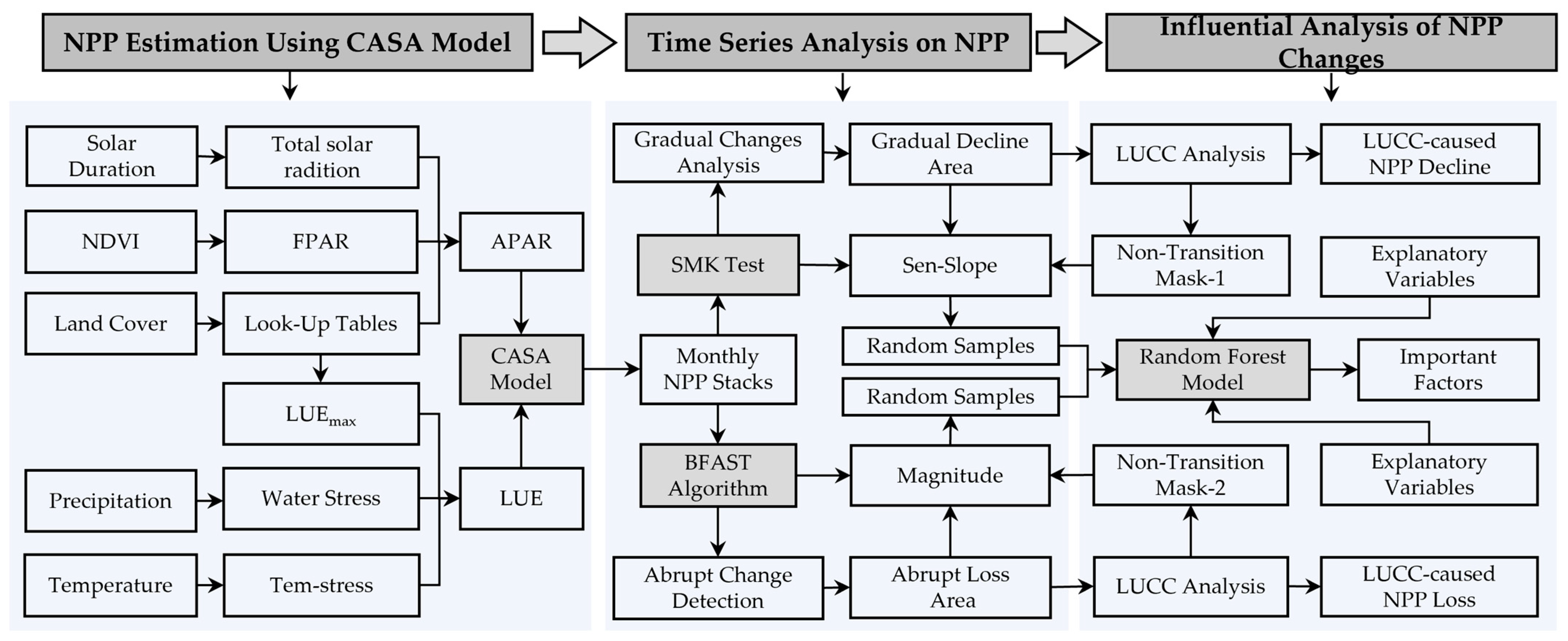
2.3. Overall Workflow

We proposed a detailed research route, as shown in Figure 2, to achieve our research objectives. We divided our research into three parts: the NPP estimation, the NPP time series analysis, and the influential factor analysis. We first generated a wall-to-wall monthly NPP time series from 2000 to 2019 based on the CASA model and various inputs at 250 m. Secondly, we utilized the Seasonal Mann–Kendall (SMK) test and Breaks For Additive Season and Trend (BFAST) approach to detect gradual and abrupt changes in the NPP time series, respectively. Thirdly, we analyzed the driving forces of NPP changes from the perspectives of land use and land cover changes, climatic factors, terrain conditions, and human activities.

2.4. Monthly NPP Estimates Based on the CASA Model

We utilized the CASA model to estimate the monthly NPP of Shandong Province. The CASA model combines a series of input parameters that can be broadly categorized into three groups: climate data (solar radiation, temperature, and precipitation), vegetation data (leaf area index and FAPAR), and biophysical parameters (maximum Light Use Efficiency, stress coefficient of water, and temperature). Here, we conceptualized the workflow, as shown in Figure 3, to represent the primary NPP estimation procedures and key parameters. More detailed equations can be found in the following sections.

In general, NPP is calculated by Absorbed Photosynthetically Active Radiation (APAR) absorbed by plants and a light utilization efficiency (ε) as follows:

$$\mathrm{N}\mathrm{P}\mathrm{P}(x,t)=APAR(x,t)\times \epsilon (x,t)$$

(1)

where NPP(x,t) is the net primary productivity (gC/m²) at a given location x at time t; APAR(x,t) is the Absorbed Photosynthetically Active Radiation (MJ/m²); and ε(x,t) is the light utilization efficiency (gC/MJ).

2.4.1. APAR Absorbed by Vegetation

APAR absorbed by vegetation is related to the proportion of total solar radiation (SOL) and Fraction of Photosynthetically Active Radiation (FPAR) absorbed by vegetation. It can be obtained as follows:

APAR(x,t) = SOL(x,t) × FPAR(x,t) × 0.5

(2)

where SOL(x,t) is the total solar radiation (MJ/m²) at x pixel in month t; FPAR is the absorption ratio of vegetation to incident photosynthetically active radiation; and constant 0.5 represents the proportion of solar effective radiation that varies among vegetations [10]. Given that MOD13Q1 selected the best available pixel values from the 16 days with low clouds, low view angle, and the highest VI value, we did not conduct further adjustments to address the background interference and signal saturation issues.

2.4.2. Calculation of Light Utilization Efficiency

Light utilization efficiency is affected by temperature and moisture and is obtained by multiplying the maximum light energy utilization rate by the constraints of temperature and moisture [46,47]. The simulation results of the maximum light utilization efficiency of typical vegetation in China were collected from [48]. Light utilization efficiency (ε) can be obtained as follows:

ε(x,t) = T_ε1(x,t) × T_ε2(x,t) × W_ε(x,t) × ε_max

(3)

where ε_max is the maximum light utilization efficiency of vegetation under ideal conditions (gC/MJ); T_ε1 and T_ε2 represent the stress effects of low- and high-temperature conditions on light utilization efficiency; and W_ε is the water stress coefficient, which reflects the restriction of carbon sequestration capacity of vegetation under drought or humid conditions. The stress coefficients were calculated following Zhu et al. [48], as shown in Supplementary Table S1.

2.5. Validation of NPP Estimation

Validating the accuracy of NPP estimation is a tricky issue, given the absence of in situ measurements within the study area. To address this limitation and assess the reliability of the CASA model outputs, we employed a two-pronged validation strategy. First, we carried out a pixel-level comparison with established NPP products, MOD17A3HGF and GLASS. To ensure spatial and temporal consistency for the analysis, our monthly CASA estimates were aggregated to annual values and resampled to a 500 m spatial resolution to match the established products. We randomly selected 10,000 pixels within the study area, focusing on areas with consistent land cover types across a five-period analysis using the GLC_FCS30 land cover maps. This approach minimizes the impact of land cover change on the comparison. Linear regression analysis was performed on the co-located pixels from each product. The coefficient of determination (R²) and root mean square error (RMSE) were calculated to quantify the agreement between the CASA estimates and the established NPP products. Second, we compared our estimates with the existing literature (please see Supplementary Table S3). The corresponding temporal periods from these studies were identified first, and then NPP statistics were calculated from our estimates during these specific periods, allowing for a direct comparison with previously reported values. This two-fold validation approach can provide insights into the reliability of our CASA estimates within the context of the study area.

2.6. Time Series Analysis of NPP Decrease

In this study, we focus on NPP decrease in terms of negative trend and anomaly reduction within monthly time series (see Figure 4a). We noted that anomalies in the data can also lead to a negative trend if the anomalies are large in magnitude or occur consistently over time (see Figure 4b). A negative trend reflects a general direction of change in the data, but it does not necessarily mean that every individual data point will be an anomaly. There can still be periods of stability or even slight increases within an overall downward trend. Here, we defined the gradual decline from the trend perspective, which refers to locations where a sustained decrease has occurred over a 20-year NPP time series. We considered it to represent a broader, long-term direction of NPP decrease. The abrupt loss was defined from the anomaly perspective, which refers to locations where significant and rapid reduction in NPP values over a relatively short period and last a certain time (to isolate from noise). The trend analysis was conducted based on the SMK test, aiming to quantify the monotonic change direction considering the different NPP distributions for different seasons, while the anomaly analysis was to detect abrupt changes in NPP time series based on a change detection algorithm called BFAST, proposed by Verbesselt et al. [49].

2.6.1. Gradual Change Detection Using the Seasonal Mann–Kendall Test

The SMK test is an extension of the Mann–Kendall (MK) test, which is a nonparametric test that does not require the data to be normally distributed. Unlike the MK tests that might miss trend changes masked by seasonal fluctuations, the SMK test explicitly considers seasonality and removes the impact of seasons in monthly resolution data. It can identify periodic data consistently increasing or decreasing over time, regardless of the rate of change. It has been widely used to detect gradual shifts in variables like seasonal temperature trends or long-term changes in vegetation cover. The specific analysis based on the monthly NPP time series is as follows:

Construct the annual NPP time series:

$$NPP={(X}_1,X_2,\dots ,X_{12})$$

(4)

$$X_i={(x}_{i1},x_{i2},\dots ,x_{i{n}_i})$$

(5)

where X is the full sample, consisting of subsamples $X_1$ to subsamples $X_{12}$ (one per month), and each subsample $X_i$ contains annual values from month $i$. Suppose that H0 represents a sample in which the data in this time series are independent and the random variables are equally distributed, with no linear trend.

For all $i,j\le n$ and $i\ne j$, calculate the statistic $S_i$ for subsample $X_i$

$$S_i={\sum }_{k=1}^{n_i-1}{\sum }_{j=k-1}^{n_i}sgn(x_{ij}-x_{ik})$$

(6)

$$sgn(\theta )=\left\{\begin{array}{c}1if\theta >0\\ 0if\theta =0\\ -1if\theta <0\end{array}\right.$$

(7)

When n ≥ 8, the statistic $S_i$ roughly follows a normal distribution, and its mean is 0. When there are the same values in n, the formula for calculating the variance is

$$VAR(S_i)=\frac{n_i(n_i-1)(2n_i+5)-{\sum }_{t_i}{t}_i(t_i-1)(2t_i+5)}{18}$$

(8)

where $t_i$ is the number of identical values in the subsample $X_i$.

Define $S^{\prime }={\sum }_{i=1}^{12}{S}_i$, then the variance can be obtained as follows:

$$VAR(S^{\prime })={\sum }_{i=1}^{12}VAR\left(S_i\right)+{\sum }_{i=1}^{12}{\sum }_{l=1}^{12}COV\left(S_i{S}_l\right)$$

(9)

Finally, the Z value of the standard normal variable is obtained:

$$Z=\left\{\begin{array}{c}\frac{S^{\prime }-1}{\sqrt{VAR\left(S^{\prime }\right)}}if{S}^{\prime }>0\\ 0if{S}^{\prime }=0\\ \frac{S^{\prime }+1}{\sqrt{VAR\left(S^{\prime }\right)}}if{S}^{\prime }<0\end{array}\right.$$

(10)

If the absolute value of Z is greater than or equal to 1.645, 1.96, and 2.576, it means that the significance test of 90%, 95%, and 99% confidence degree has been passed, respectively. The H0 hypothesis is not valid, and there is a trend in the sequence. A positive Z indicates an upward trend, and a negative Z indicates a decreasing trend.

2.6.2. Abrupt Changes Detection Based on the BFAST Algorithm

The BFAST algorithm detects abrupt changes by identifying stable historical changes and establishing models. It can detect breakpoints with high precision and flexibility, which makes it suitable for various applications such as forest disturbance mapping, water quality monitoring, vegetation health, and so forth. It deconstructs a time series into three individual components, i.e., the trend component, seasonal component, and residual component (Figure 4). By separating these components, BFAST isolates the breakpoints within the trend, revealing significant shifts in the underlying process. The outputs of BFAST are means, break time, and magnitudes, respectively, among which magnitudes can represent the intensity of change in the abrupt change point. In this paper, we used the change magnitude to represent the intensity of abrupt change in the NPP time series. The specific analysis methods are as follows [50]:

(1)

Decompose the NPP time series into three components and assume linearity in trends and moderate seasonality in observations y_t at time t:

$$y_t=T_t+S_t+{\epsilon }_t$$

(11)

$$y_t={\alpha }_1+{\alpha }_2+{\sum }_{j=1}^k{\gamma }_{j}sin(\frac{2\pi jt}{f}+{\delta }_j)+{\epsilon }_t$$

(12)

where $y_t$ is the observation data in the time range t; $T_t$ is the trend component; $S_t$ is the seasonal component; ${\epsilon }_t$ is the residual component; ${\alpha }_1$ and ${\alpha }_2$ are the trend coefficients; ${\gamma }_j$ is the amplitude; f is the frequency; and ${\delta }_j$ is the number of segments, where ${\gamma }_j$ and ${\delta }_j$ are unknown terms and f are known terms.

(2)

The above models can be written as standard linear regression models:

$$y_t=x_t^T\beta +{\epsilon }_t$$

(13)

$$x_t^T=\{1,t,sin(\frac{2\pi t}{f}),cos(\frac{2\pi t}{f}),\dots ,sin(\frac{2\pi kt}{f}),cos(\frac{2\pi kt}{f}\left)\right\}$$

(14)

$$\beta =\{{\alpha }_1,{\alpha }_2,{\gamma }_{1}cos({\delta }_1),{\gamma }_{1}sin({\delta }_1),\dots {\gamma }_{k}sin({\delta }_k),{\gamma }_{k}sin({\delta }_k\left)\right\}$$

(15)

where k is a harmonic term, and a higher k value indicates a shorter periodic change. β is an unknown parameter set.

(3)

According to the established seasonal trend model, the structural changes of the time series were detected by MOSUM (moving sums of the residuals), and the calculation formula is

$${MO}_t=\frac{1}{\widehat{\sigma }\sqrt{n}}{\sum }_{s=t-h+1}^t(y_s-x_s^T\widehat{\beta })$$

(16)

where $\widehat{\beta }$ is the estimated value of $\beta$ in the period t = 1,2, …, n, h is the bandwidth of the MOSUM, and is usually selected relative to the size of the historical sample; $\widehat{\sigma }$ is the variance estimate; and n is the historical observation period. If the model remains stable, the MOSUM should be close to zero, and only random fluctuations occur. If the series deviates from zero and exceeds the 95% significance boundary, we define the time series as a breakpoint, namely abrupt change.

The SMK test and BFAST analysis were carried out independently. However, because abrupt loss can cause a monotonic decrease trend, here we roughly designated overlapped pixels as abrupt changes for the subsequent analysis. Our analysis revealed an overlap area of approximately 1161.25 km² that represents 8.9% of the total gradual decline area and 92.6% of the abrupt loss area, respectively. Therefore, through the SMK analysis, we obtained a wall-to-wall S statistic to indicate the trend direction and strength of NPP gradual changes, while we used the break magnitude derived from BFAST to indicate the strength of the latest NPP shift. Since the BFAST requires a specific window to fit the linear regression model, we used the first 10-year monthly NPP observation as the training data; thus, the BFAST analysis can only detect abrupt changes after 2009.

2.7. Statistical Analysis

We implemented land cover change analysis and Random Forest modeling to identify the influential factors driving NPP change in our study area. We first determined the pixels that experienced land cover changes and extracted the overlapped ones that featured gradual or abrupt change. For these pixels, we created transition matrices and used a Sankey diagram to depict the flows of land cover changes. For the rest of the change pixels with consistent land cover types, we adopted a Random Forest model to identify the influential factors and quantify their relative importance in driving gradual or abrupt NPP changes. Considering that the driving factors may differ substantially by vegetation type and NPP change type, we established six Random Forest models for the three categories of vegetation types (i.e., farmland, forests, and shrub-grasslands) to address the two types of NPP changes.

2.7.1. Explanatory Variable

We obtained a series of spatial datasets from multiple perspectives, such as climate, vegetation, human activity, and terrain conditions, to investigate how these factors influence NPP changes (

Table 2. Explanatory variables to explain abrupt loss and gradual decline in monthly NPP time series from 2000 to 2019.

Model	Explanatory Variable	Description
Abrupt loss	pre	Mean annual precipitation of two years before the loss year
	tmn	Minimum temperatures of two years before the loss year
	tmx	Maximum temperatures of two years before the loss year
	Δtmp	Trend of monthly temperature for 2000–2019
	Δpre	Trend of precipitation for 2000–2019
	ΔEVI	Trend of monthly EVI trends for 2000–2019
	Breaks_EVI_mean	Mean EVI of two years prior loss year
	Breaks_EVI_cv	Coefficient of variation of EVI prior loss year
	Breaks_EVI_acf	Auto-correlation function of EVI since 2000 to the loss year
	Night light	Night light intensity in 2019 of a given pixel
	People	The total population in 2019 of a given pixel
	Road distance	The nearest distance to a road of a given pixel
	Elevation	Elevation in meters
	Slope	Slope in degree
Gradual decline	pre	Mean annual precipitation for 2000–2019
	tmp	Annual accumulated temperature during the growing season
	Δtmp	Trend of monthly temperature for 2000–2019
	Δpre	Trend of precipitation for 2000–2019
	ΔEVI	Trend of monthly EVI trends for 2000–2019
	EVI_cv	Coefficient of variation of monthly EVI for 2000–2019
	EVI_acf	Auto-correlation function of EVI for 2000–2019
	Night light	Night light intensity in 2019 of a given pixel
	People	The total population in 2019 of a given pixel
	Road distance	The nearest distance to a road of a given pixel
	Elevation	Elevation in meters
	Slope	Slope in degree

). Those datasets were processed to be consistent with the spatial and temporal resolution of the NPP dataset in this study. NPP was derived from the CASA model, which involved climate and vegetation factors, so we used second-order statistics derived from the raw datasets as the indicator. For the gradual changes, we generally applied the overall statistics, such as the mean annual values or trend indicators from the whole time series, as the predictor variables. Abrupt changes required an explicit temporal context for the environmental variables. Thus, we generated pre-change predictors according to the abovementioned break timing information. A detailed description and relevant information on the explanatory variables can be found in Table 2.

2.7.2. Random Forest Modeling

We used the Random Forest model, which is a powerful ensemble machine learning algorithm, to fit the relationships between the abovementioned explanatory variables and the response variables that can indicate NPP gradual changes and abrupt changes. The Random Forest model falls under the bagging category, wherein multiple weak classifiers are combined to produce a final result through voting or averaging. This approach enhances the overall accuracy and generalization performance of the model. We used NPP change pixels that did not experience land cover change as the input samples to fit six Random Forest models. The total sample size was approximately 130,000 pixels, with 60% used as training data and the rest as validation data. Such a large number of training samples can guarantee that the model avoids overfitting. Random Forest can provide accuracy-based and Gini-based measures for ranking variable importance; here, we used the first measure as the criterion. This measures how much the accuracy decreases for a particular variable when it is excluded from splitting in a tree. We adopted partial dependence to interpret how a particular variable affects the response variable while averaging out the influence of all other variables. The GridSearchCV method in the scikit-learn package (version 1.3.1) was used to search for the best parameters of the model and determine the relative importance of the model features. A partial dependency analysis was carried out according to the obtained model to explore the influence of various variables on the model under different conditions and how these variables affect the model.

3. Results

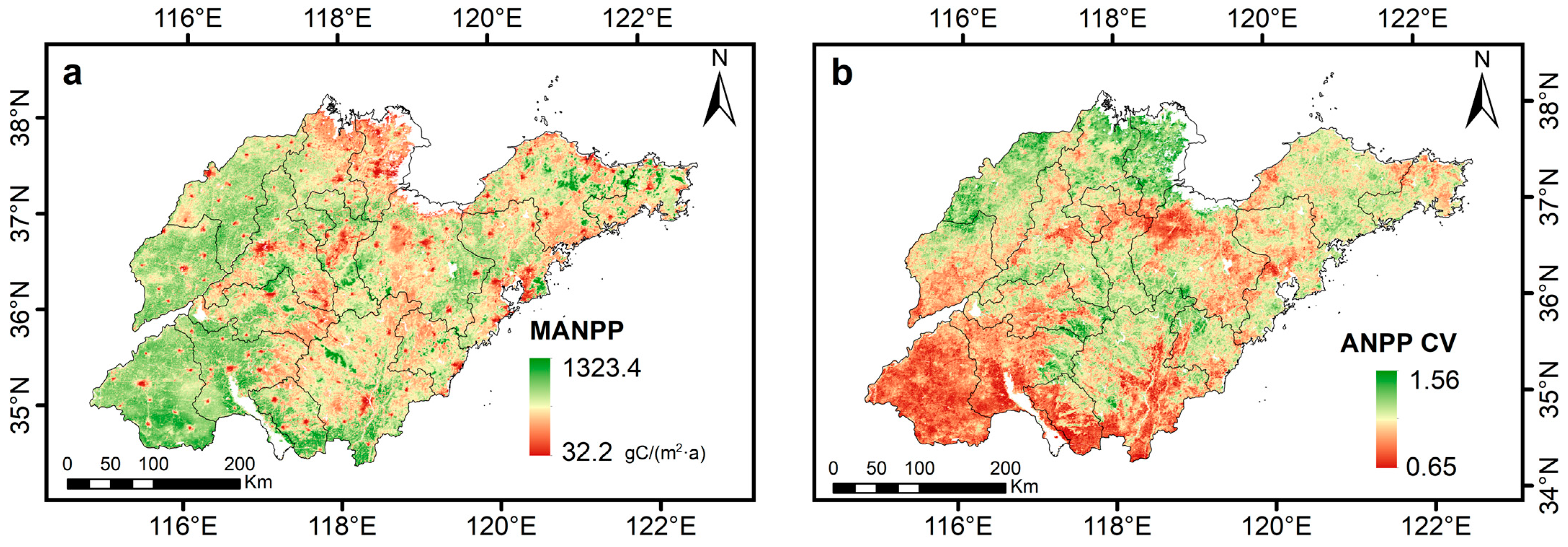
3.1. Estimates of NPP for 2000–2019

We generated a monthly NPP product for Shandong Province from 2000 to 2019 at 250 m spatial resolution. The pixel-level validation (see Supplementary Figure S1) indicated our estimates were better aligned with the GLASS NPP product (R² = 0.68, RMSE = 114.00) than the MOD17A3HGF product (R² = 0.59, RMSE = 360.87). The range of NPP values assessed in this study exhibits slight discrepancies compared to those reported in the existing literature. However, these differences were acceptable as they do not involve orders-of-magnitude differences. By integrating monthly NPP products into a mean annual NPP (MANPP) product and conducting a statistical analysis, we found that the MANPP in Shandong Province was 503.45 gC/(m²·a) (SD = 118.28 gC/(m²·a), Figure 5a) and the range of total annual NPP was about 0.06–0.08 Pg. The MANPP of farmland, forest, and grassland were 514.95 gC/(m²·a) (SD = 105.06 gC/(m²·a), Figure 5b), 708.13 gC/(m²·a) (SD = 114.77 gC/(m²·a), Figure 5c), and 534.87 gC/(m²·a) (SD = 96.05 gC/(m²·a), Figure 5d), respectively. Their contributions to the total MANPP of the whole study area in 2000–2019 were approximately 81.5–82.1%, 2.1–2.8%, and 5.7–6.1%, respectively. We also adopted a series of MK tests to demonstrate the trends of annual NPP in Shandong Province. The results showed a pronounced and consistent increasing trend (Slope = 0.23, p < 0.05) of total annual NPP for the whole province. Among the three primary vegetation types, forests exhibited the most rapid growth at 255.58 gC/(m²·a) (Slope = 0.44, p < 0.05), followed by grassland 165.67 gC/(m²·a) (Slope = 0.32, p < 0.05), and farmland 90.27 gC/(m²·a) (Slope = 0.25, p < 0.05).

The spatial distribution of NPP in Shandong Province has a clear regularity, with lower NPP observed in the central region and higher values found in the western part. This distribution is influenced by the spatial arrangement of land cover types and topography. In the western region, farmland dominates the landscape, exhibiting a continuous pattern of high NPP. In the central area, forested slopes prevail within Mount Tai and the Jiaodong Mountains, resulting in a fragmented distribution of areas with elevated NPP values. The discrete low-value areas predominantly occur in urban regions, while the continuous low-value areas are primarily distributed across the northern region (saline land), the grassland of the central region (hills and barren mountains), and certain greenhouse agricultural zones (Figure 6a). By analyzing the variation in annual NPP in terms of coefficient of variation (CV), we showed that about 82.2% of the study area has CV values less than 1. The areas with high CV values were predominantly distributed in the northwest and central regions, where the primary vegetation types in 2020 were farmland and grassland (Figure 6b). The areas with low variation exhibited a continuous pattern in the southwestern and southern parts, as well as the central–northern part, where the low CV areas were distributed in a banded pattern that was composed of farmland and forest.

3.2. Time Series Variation Characteristics of NPP

The monthly time series of NPP were used for change detection and monotonicity trend analysis by integrating BFAST and SMK test algorithms. The results showed that about 3.89% of the total study area experienced abrupt loss between 2010 and 2019 (Figure 7). This was mainly in the coastline of the northern part of the study area and surrounding urban areas (such as Jining, Jinan, Linyi, and Rizhao), indicating that a change in land cover type, especially urban expansion, was the main factor causing the abrupt loss of NPP. On the other hand, the SMK test revealed that approximately 69.67% of the study area exhibited a significant monotonic increasing trend from 2000 to 2019. The predominant land cover types were farmland, grassland, and forest, which accounted for about 80.7%, 7.2%, and 2.3%, respectively, of the NPP increase area. More importantly, we found that approximately 8.46% of the total area showed a significant monotonic decreasing trend. The large, continuous distribution area was mainly located in the border area of Weifang, Zibo, Binzhou, and Dongying, while the scattered distribution area was mainly distributed around the cities. Based on these change pixels, we further investigated the NPP balance in 2010–2019. The cumulative NPP gain (about 1.41 × 10⁷ t C) in the monotonically increasing area (from SMK test) was 1.39 × 10⁷ t C more than the cumulative NPP loss (about 1.40 × 10⁵ t C) in the monotonically decreasing area (from SMK test) and abrupt decreasing area (from BFAST). The net gain in those areas indicating the eroded amount of NPP can be offset by the area of gradual increase. The statistics on the area of NPP changes by land cover types can be found in Supplementary Table S2.

3.3. Influential Analysis of Spatiotemporal Variation of NPP

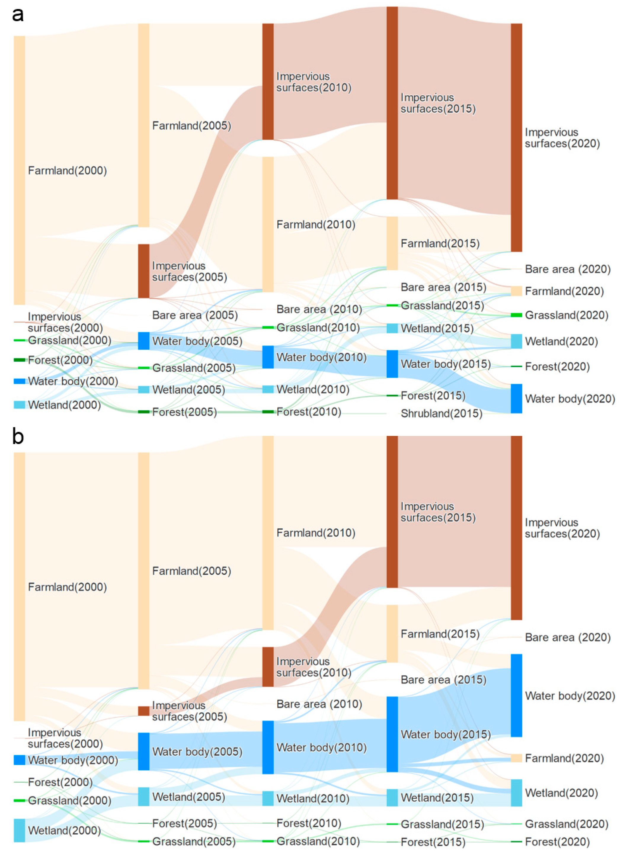
3.3.1. NPP Changes Caused by LULC Transition

Our analysis revealed that approximately one-third of the areas exhibiting gradual decline were due to land cover changes (Figure 8a). The majority of these changes were transitions from farmland to urban areas, particularly noticeable from 2000 to 2015 (Figure 9a). Notably, there was also a conversion from forest to farmland, especially from 2010 to 2015. Changes in NPP within these areas were largely attributable to shifts in crop type or farming patterns. Approximately 70.0% of the regions identified as undergoing abrupt changes experienced transitions in LULC (Figure 8c). The predominant transition pathway was from farmland to impermeable surface, a shift primarily driven by urban expansion (Figure 9b). A minor proportion of land, primarily composed of vegetation-dominated types such as forests and grasslands, was converted into urban areas (Figure 8b,d). The remaining regions, which did not undergo LULC change, were primarily farmland (approximately 78.6%).

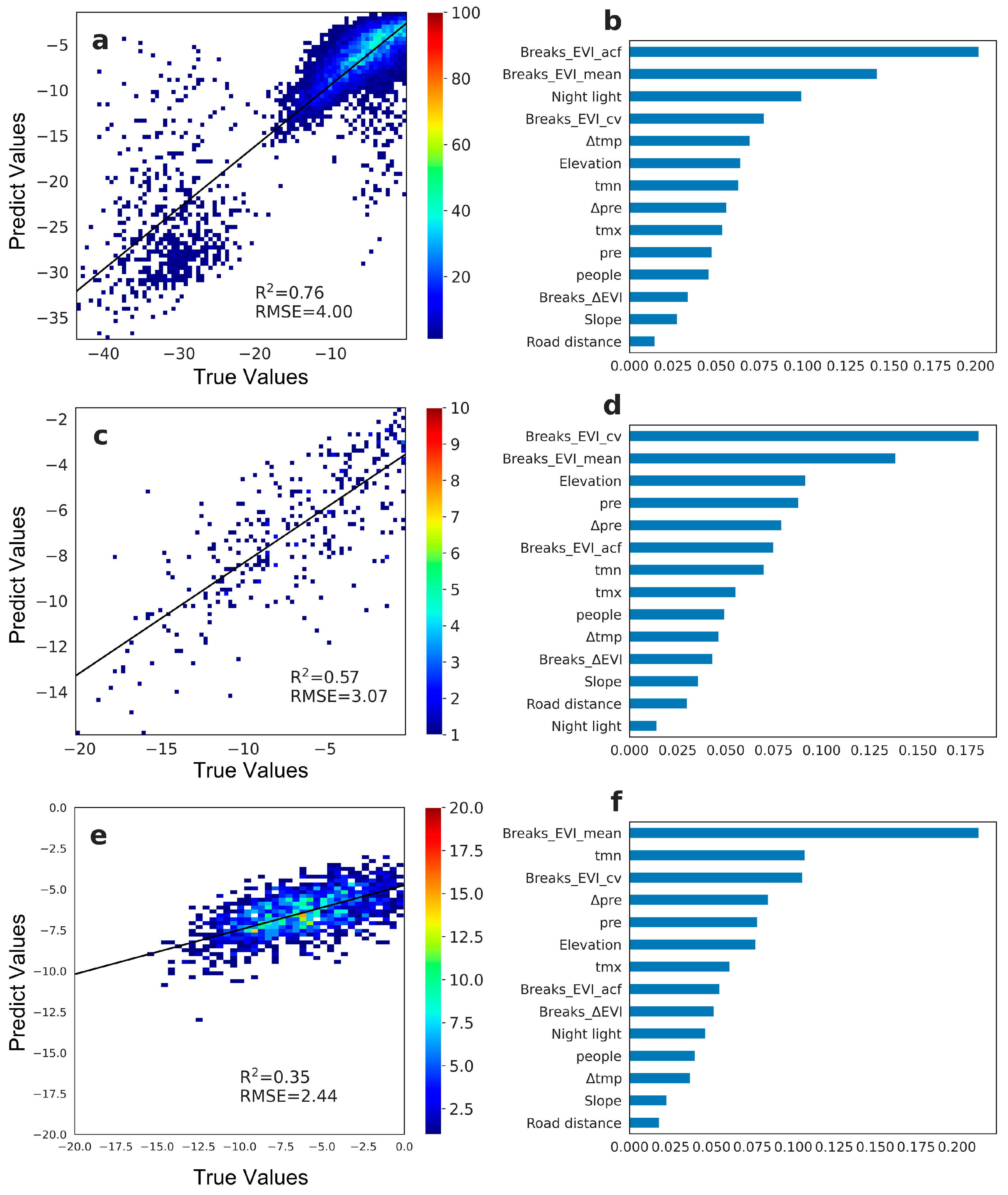
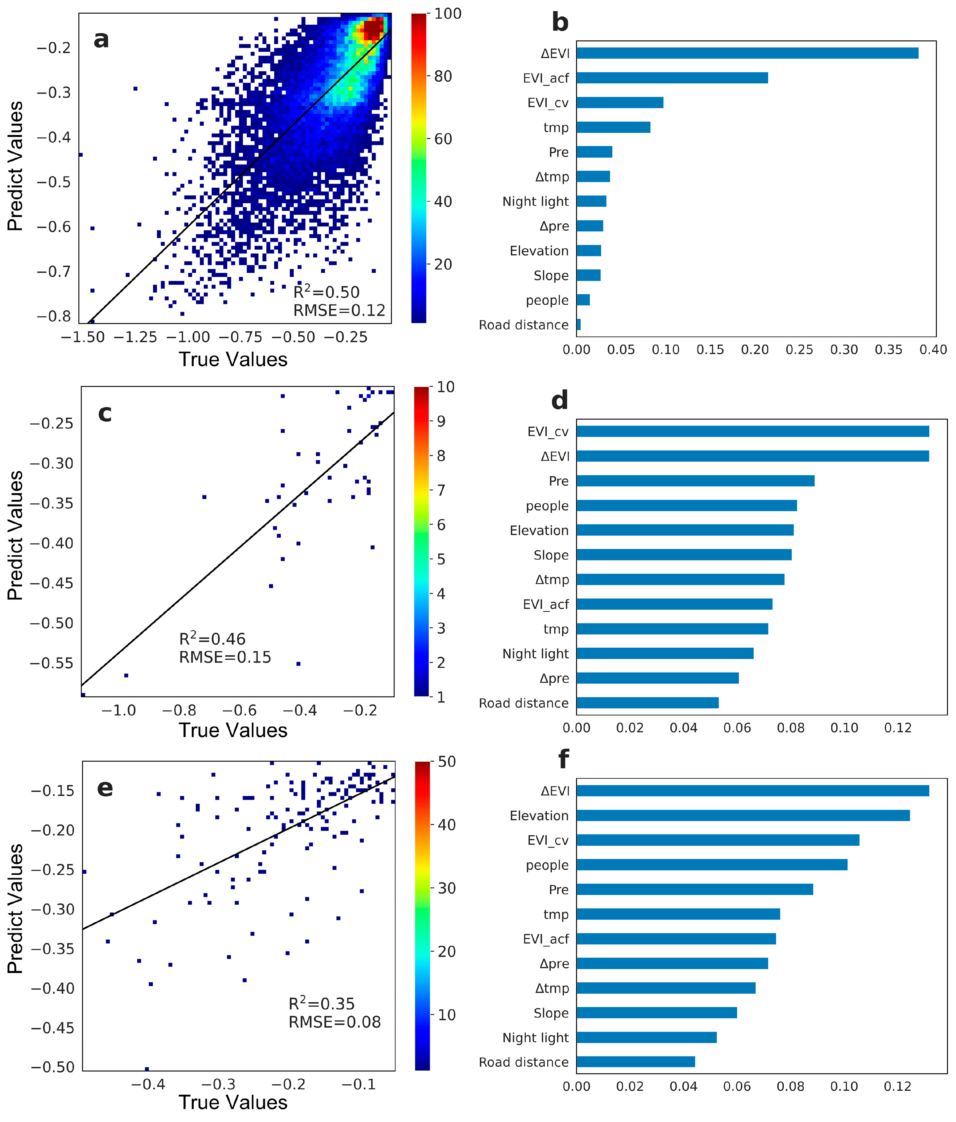
3.3.2. Influential Analysis of NPP Abrupt Loss without LULC Transition

We employed the Random Forest model to investigate the drivers of NPP abrupt changes across forest, farmland, and grassland pixels (see Figure 10). The model demonstrated robust predictive capabilities, explaining 76%, 57%, and 43% of the magnitude variations of NPP abrupt changes in farmland, forest, and grassland, respectively. For farmland, indicators related to the EVI, specifically EVI_mean, EVI_acf, and EVI_cv, which reflect vegetation status, were of high relative importance, contributing approximately 44.5% to the total relative importance. Notably, EVI_acf and EVI_mean accounted for 20.2% and 14.3% of the relative importance, respectively, before the abrupt change. Night light intensity, a proxy for human activities, emerged as another significant variable explaining the abrupt changes in farmland NPP, suggesting that urbanization is a key factor driving these abrupt changes. Additionally, temperature-related variables (Δtmp and tmn), precipitation, and altitude also demonstrated a certain degree of importance, accounting for 13.2%, 4.7%, and 6.5% of the relative importance, respectively. In the case of forests, the EVI-related indices (EVI_cv and EVI_mean) had a relative importance of 18.2% and 13.9%, respectively. Elevation and precipitation were the second most important factors, contributing 9.1% and 8.8% to the relative importance, respectively. These results suggest that vegetation status and environmental conditions are the primary determinants of the abrupt change magnitudes in forest NPP. Similar to farmland and forest, EVI_mean and EVI_cv were significant factors in explaining the magnitude of abrupt changes in grassland, contributing 21.3% and 10.6% of the relative importance, respectively. Additionally, precipitation trends, minimum temperature, elevation, and precipitation, which characterize drought, contributed 8.4%, 10.7%, and 7.7% of the relative importance, respectively. These results indicate that the interactions between climate, topography, and vegetation dominate the abrupt changes in grassland NPP.

3.3.3. Influential Analysis of NPP Gradual Decline without LULC Transition

In this study, three Random Forest models were developed and demonstrated reasonably high training accuracy (see Figure 11). These models could explain 50%, 46%, and 35% of the trend variation for farmland, forest, and grassland pixels, respectively. The model results indicated that ΔEVI, representing the trend of vegetation status, was the most critical factor in explaining the monotonic changes in NPP across the three ecosystem types. It contributed 44.1%, 15.7%, and 16.8% of the relative importance, respectively. Climate-related factors, such as temperature, precipitation, and temperature trends, made significant but limited contributions to NPP declines in farmland and forests. In contrast, altitude and population were significant factors in NPP declines in grassland systems, each contributing approximately 11% of the relative importance. Two indicators of human activity intensity, namely night lights and the shortest distance from the road, along with the slope, did not exhibit high relative importance for the attenuation of NPP. This finding suggests that human activities and topographic slope did not significantly impact the attenuation of NPP.

4. Discussion

4.1. Spatiotemporal Variations in NPP in Shandong Province

In this study, we generated a time series of monthly NPP datasets and analyzed the spatiotemporal variations in terms of patterns, trends, changes, and balance in Shandong Province. Benefiting from the combined strength of the CASA model and MODIS NDVI product, we found that our estimation was well aligned with the GLASS NPP product (Supplementary Figure S1) and other studies carried out in the same province and similar ecosystems (Supplementary Table S2) [5,49,50,51]. Among the primary land cover types, as expected, the forests had a stronger carbon sequestration ability than cropland and grassland, according to our estimation. Although forests only occupied a limited area (1.8%), they contributed a mean total of 708.38 gC/(m²·a), which accounted for about 2.6% of the total NPP. The study area did not have significant regions of grassland or shrubland, and therefore, they only contributed a limited portion of ANPP. According to the land cover conditions, grassland and shrubland are generally distributed in hilly areas where the soil is shallow and infertile, which further worsens plant development. The cropland contributed a considerable proportion of 81.60% of the total NPP, but it also has a high intra-annual variation of vegetation types. The most productive croplands were distributed in the western and southern regions of our study area [38], where we did not observe much NPP decline or loss. They are significantly affected by the temperate ocean and monsoon climate with suitable hydro-thermal conditions, which are conducive to vegetation growth [51].

Spatially, the urban and surrounding areas exhibit remarkably low MANPP, as expected. A high degree of urbanization will decrease vegetation productivity through the direct loss of vegetation [35]. Besides the urban area, the north plain area that belongs to the Yellow River Delta represents low MANPP due to high soil salinization [52]. Although most of the land in this area was used for agriculture, the impaired nutrient uptake and water stress can directly stunt plant growth and thereby reduce biomass production. The hilly areas in the central and eastern parts of the study area also exhibited a similarly low vegetation MANPP. Sparse and fragmented vegetation, coupled with unfavorable water drainage conditions and infertile soil, leads to such a situation [53]. As a comparison, the hilly area covered with forests had a high MANPP, implying that high carbon sequestration potential can be achieved if ecosystems can be managed adaptively based on local conditions.

Temporally, we observed a slowly increasing but statistically significant trend from 2000 to 2019, suggesting that the total ANPP of the whole study area was enhanced, as found in other studies [54,55,56,57]. From our results, it was clear that there were more areas with an ANPP growth trend than with an ANPP decrease, which produced a net increase in NPP for the whole province. Although the evaluation results imply an optimistic estimation, we still need to pay attention to areas with significant NPP decline or even loss in the study area. Through the spatial distribution of NPP changes, we see that ANPP decline or loss mostly occurred around urban areas, driven by urban expansion. However, there were exceptions; for example, we found a large and spatially continuous area with declined ANPP in the central–north part of the province, which was caused by the conversion of open fields to plastic greenhouses. The plastic film of the greenhouses sheltered the spectral signal of crops and thereby decreased the NDVI values and the final NPP estimation. But, there is no doubt that these greenhouses have productivity values far higher than the estimated results. We noted such underestimation here, but we cannot fix the problem due to being unable to obtain true spectral information.

4.2. Factors Monotonically Diminishing NPP Variation

Benefiting from the explanatory strength of partial dependence curves generated from the Random Forest model (Figures S2–S7), we can interpret the influence of environmental variables on the NPP trend. Here, we only focus on the selected variables used to establish the Random Forest model and do not discuss the direct impacts of land cover changes on NPP trends. The threshold phenomena observed in partial dependence curves can offer valuable insights into the mechanisms by which NPP responds to environmental changes. However, many factors may cause fluctuations and thresholds in partial dependence curves, such as the interaction between variables, the distribution and sample size of training data, and the goodness of model fitting. We believe that the general patterns revealed by the partial dependence curves are highly reliable, whereas the specific details of the thresholds are more vulnerable to the impact of diverse confounding elements. Therefore, we focus primarily on how NPP reduction responds to environmental changes rather than extensively discussing the threshold effects present in the partial dependence curves.

For the cropland, our results indicated that the vegetation conditions in terms of EVI-related variables showed positive impacts (Figure S2a–c), while the rest of the variables either posed negative but slight influences (i.e., temperature) or were of negligible importance. This demonstrated that climatic factors have limited influence on agriculture productivity, which benefits from reasonable management measures related to labor inputs and robust irrigation systems in this province [58]. For natural ecosystems, such as forest and grassland, the EVI-related variables also represent positive influences (Figures S3 and S4a–c). However, we noted that climate-related variables (i.e., precipitation and temperature) played more important roles and had more straightforward relationships than the quality of farmland [59]. Too much precipitation decreased the ANPP of these two ecosystems, while increased temperature generally slowed down ANPP decline but differed substantially between them (Figure S3 and S4k,l). We considered that the study area has a temperate monsoon climate, with rain and heat at the same time. A rise in temperature can promote respiration and transpiration [60], accelerate nutrient decomposition, shorten leaf lifespans, reduce root ranges, and cause surface droughts that affect vegetation growth [61,62]. Our results showed that the NPP decline in grassland was more sensitive than forest in terms of responding to changes in temperature, which may be due to forest being more resilient to changes in temperature than grassland. A slight increase in precipitation can maintain a positive ANPP trend, but a higher increase may suppress vegetation productivity since excess soil moisture can drown plant roots and limit their ability to absorb oxygen and nutrients [63]. For grassland, we noticed that population density and elevation are also important factors. Areas with higher population density had more nutrient availability, thus causing higher productivity of grassland. As to the terrain condition, the elevated area in our study area is usually hilly with sparse vegetation and high rock or bare soil exposure. The inherent vulnerability of these ecosystems, compounded by resource limitations resulting from unfavorable terrain conditions, is likely to exacerbate the decline in NPP.

4.3. Factors Driving Vegetation NPP Abrupt Loss

There is no doubt that land-use-derived vegetation changes caused the most abrupt loss of NPP, among which farmland loss due to urban expansion and aquatic ecosystem restoration are the primary factors. We noted that environmental changes and LULC transition may have compound effects on NPP abrupt loss, but we considered that LULC transition plays a dominant role in controlling NPP changes. By contrast, the influence of other factors on NPP is predominantly gradual and long-term. However, we also acknowledge that the strict thresholds we adopted in the BFAST model may lead to the omission of some abrupt loss pixels, whose NPP decrease was also caused by LULC transition but were featured with weak changes. These pixels also represented monotonic reduction as detected in the SMK test but been misclassified as gradual declines. This can partly explain why a significant proportion of farmland conversion to urban areas resulted in gradual NPP declines in our results (Figure 9a). Since we first detected NPP changes solely based on NPP time series analysis and then tracked the LULC transition within these areas, we thought the accuracy of land cover maps could also influence the analysis of NPP abrupt loss. Additionally, the spatial aggregation process applied to land cover data may have introduced uncertainties, potentially leading to inconsistencies in land cover type results for areas adjacent to agricultural and urban regions due to independent aggregation procedures for each time period.

In this study, we quantified the amount of decreased ANPP that is straightforward and reasonable. Therefore, here, we pay more attention to the NPP losses that were not attributed to land cover conversion. Through the outputs of NPP loss models, we generally found that the vegetation conditions in terms of EVI-derived variables were important for explaining the magnitude variability of NPP loss. However, farmland, grassland, and forests represent different responses to EVI-related variables. We found that farmland and grassland with low pre-loss EVI and ACF were more likely to cause high-magnitude NPP loss (Figure S5d,f). For forests, we found that high EVI and CV were responsible for NPP loss (Figure S6d,e). The EVI of farmland was mainly driven by agricultural practices that were closely associated with human activities. Some influential factors such as farmland abandonment, crop changes, soil degradation, and greenhouse construction can either reduce vegetation cover or blur the spectral signal of vegetation and finally cause NPP loss. The farmland and grassland with lower EVI were more likely to have such problems. For forests, the NPP loss is usually owing to disturbances such as fire, insects, harvesting, and so forth [64]. Forests with high EVI mean higher fuel accumulation or timber storage; events such as fire and harvesting will lead to a further loss of NPP.

Through our analysis, we found that pre-loss climatic factors and human activities had important impacts on NPP loss. For the cropland, we found that nightlight and temperature-related variables can well explain the NPP loss magnitude. The farmland featured high NTL intensity; in other words, fields near urban or residential areas tended to have a higher magnitude of NPP losses (Figure S5b,c,h,j). Variables related to low temperatures are more important climate factors, and the results show that regions with larger temperature differences are more likely to experience high levels of NPP loss. Climate change-induced temperature variability can have a significant impact on subsequent vegetation productivity; in particular, the previous year’s low-temperature events can lead to a loss of NPP in the following year. This is related to the fact that winter wheat is the main crop in our study area [65]. The cold weather and temperature difference in winter can cause damage or loss of crops, which in turn affects the yield in the coming year (Figure S5b,c,h). Our results also showed that precipitation had very limited impacts on farmland NPP loss, which may indicate sufficient precipitation and well-developed irrigation facilities.

For forest and grassland, we found that the influences of climatic factors on NPP losses differed substantially from farmland. For forests, the maximum temperature was the most important of our selected climatic variables. The NPP loss will decrease along with maximum temperature, suggesting that climate warming may have limited impacts on forest productivity loss in Shandong Province (Figure S6c). Similarly, the positive trend of precipitation can also reduce the risk of forest NPP loss (Figure S6i). This may be because the forests in our study area are water-availability limited as they are widely distributed in hilly and montane environments where precipitation is the primary water source. This inference can also be cross-validated from the response of NPP loss to elevation; that is, elevated areas will more easily experience abrupt NPP loss. Similar responses of NPP loss to precipitation trends and elevation can also be found for grassland (Figure S7c,m).

4.4. Limitations

Our study is the first to monitor province-scale vegetation NPP changes and elucidate the underlying driving forces. Such analysis requires exhaustive spatially explicit inputs related to remote sensing datasets and environmental variables, so it comes with limitations and uncertainties. First, due to the lack of field observations of NPP that can match the long-term NPP estimates, the validation of the NPP estimation results in this study is not a site-scale validation but is carried out by comparing with established global NPP products and previous studies (see Supplementary Figure S1 and Table S3). Since this study is based on the accuracy of the CASA model shown in many previous studies [66], our confidence in the accuracy of NPP estimation is partly due to the applicability of the model and partly because the model data parameters all use published standardized data products that had undergone peer review. We noted that this does not imply the superiority of our NPP assessment over other studies. Second, in the process of estimating NPP, the vegetation index data and climate data we used have suitable temporal continuity, but it is undeniable that the spatial resolution is relatively low. Analysis at this scale is easily affected by mixed pixels. For example, for the acquisition of ecosystem types, we used spatial aggregation analysis of vegetation cover type data based on Landsat, which may cause some bias. Third, for the temporal change in NPP, in this study, we only examined two patterns of monotonously decreasing and sharply decreasing, but there may be other patterns of change in the actual NPP time series data. For example, many studies have reported multiple disturbances [67,68], but in this study, limited by the change detection algorithm, we only quantitatively analyzed the most recent disturbance in the NPP time series data and did not consider the important impact that historical disturbances may have on subsequent disturbances. Fourth, in terms of setting the driving factors, we comprehensively considered the availability of long-term gridded data related to driving factors and the explanatory power of driving factors themselves for NPP changes. We selected datasets that represent climate change, topography, and human activities. These datasets have accuracy limitations when expressing the corresponding attributes, which will inevitably have an impact on the results of this study. At the same time, the driving factors we set are also affected by subjective factors. Some data that can more finely characterize human activities may be considered for inclusion in the future in order to improve our understanding of the impact of human activities.

5. Conclusions

Vegetation NPP is a fundamental indicator of regional ecosystem health. Therefore, the monitoring of NPP dynamics and the underlying influential factors are of critical importance for improving our management of ecosystems. We generally found an upward trend of ANPP in Shandong Province: approximately 69.67% of the total area showed significant increases from 2000 to 2019. At the same time, we found that approximately 3.89% of the total area experienced abrupt loss, and 8.47% showed a monotonic decreasing trend. Through our analysis, we demonstrated that over half of the NPP loss could be attributed to land cover changes, among which the transition from farmland to urban area was the primary driver. For the area with diminished NPP but no land cover changes, we identified different influential factors of NPP abrupt loss and monotonic decline for farmland, forests, and grassland, respectively. The pre-loss vegetation condition (in terms of mean background value and temporal variation) mainly determined the magnitude of NPP loss, while the precipitation, temperature, elevation, and human activities exerted reasonable but differential impacts on those ecosystems. For the monotonic decline area, the trend of the vegetation index largely determined the rate of NPP decline. The decline in NPP in forests and grassland was significantly limited by climate and topography, while agricultural ecosystems were less affected by these factors, possibly because of human-intensive management. Our results implied that intensified land use and extreme climatic factors diminished the NPP of Shandong Province, but a broader range of positive vegetation growth trends can enhance NPP and counterbalance the decrease.

References

1. Fang, J.; Yu, G.; Liu, L.; Hu, S.; Chapin, F.S. Climate Change, Human Impacts, and Carbon Sequestration in China. Proc. Natl. Acad. Sci. USA 2018, 115, 4015–4020. [Google Scholar] [CrossRef] [PubMed]
2. Chen, T.; Peng, L.; Liu, S.; Wang, Q. Spatio-Temporal Pattern of Net Primary Productivity in Hengduan Mountains Area, China: Impacts of Climate Change and Human Activities. Chin. Geogr. Sci. 2017, 27, 948–962. [Google Scholar] [CrossRef]
3. Yang, Y.; Shi, Y.; Sun, W.; Chang, J.; Zhu, J.; Chen, L.; Wang, X.; Guo, Y.; Zhang, H.; Yu, L.; et al. Terrestrial Carbon Sinks in China and around the World and Their Contribution to Carbon Neutrality. Sci. China Life Sci. 2022, 65, 861–895. [Google Scholar] [CrossRef] [PubMed]
4. Khalifa, M.; Elagib, N.A.; Ribbe, L.; Schneider, K. Spatio-Temporal Variations in Climate, Primary Productivity and Efficiency of Water and Carbon Use of the Land Cover Types in Sudan and Ethiopia. Sci. Total Environ. 2018, 624, 790–806. [Google Scholar] [CrossRef] [PubMed]
5. Liu, Y.; Jun, Z.; Zhang, C.; Xiao, B.; Liu, L.; Cao, Y. Spatial and temporal variations of vegetation net primary productivity and its responses to climate change in Shandong Province from 2000 to 2015. Chin. J. Ecol. 2019. [Google Scholar] [CrossRef]
6. Zhao, M.; Running, S.W. Drought-Induced Reduction in Global Terrestrial Net Primary Production from 2000 Through 2009. Science 2010, 329, 940–943. [Google Scholar] [CrossRef] [PubMed]
7. Chen, P. Monthly NPP Dataset Covering China’s Terrestrial Ecosystems at North of 18°N (1985–2015). J. Glob. Chang. Data Discov. 2019, 3, 34–41. [Google Scholar] [CrossRef]
8. Yuan, W.; Cai, W.; Liu, D.; Dong, W. Satellite-based vegetation production models of terrestrial ecosystem: An overview. Adv. Earth Sci. 2014, 29, 541–550. [Google Scholar] [CrossRef]
9. Chen, F.; Li, H.; Liu, Y. Spatio-temporal differentiation and influencing factors of vegetation net primary productivity using GIS and CASA: A case study in Yuanyang County, Yunnan. Chin. J. Ecol. 2018, 37, 2148–2158. [Google Scholar] [CrossRef]
10. Piao, S.; Fang, J.; Zhou, L.; Guo, Q.; Henderson, M.; Ji, W.; Li, Y.; Tao, S. Interannual Variations of Monthly and Seasonal Normalized Difference Vegetation Index (NDVI) in China from 1982 to 1999. J. Geophys. Res. 2003, 108, 2002JD002848. [Google Scholar] [CrossRef]
11. Shi, Z.; Wang, Y.; Zhao, Q.; Zhang, L.; Zhu, C. The spatiotemporal changes of NPP and its driving mechanisms in China from 2001 to 2020. Ecol. Environ. Sci. 2022, 31, 2111–2123. [Google Scholar] [CrossRef]
12. Lin, H.; Feng, Q.; Liang, T.; Ren, J. Modelling Global-Scale Potential Grassland Changes in Spatio-Temporal Patterns to Global Climate Change. Int. J. Sustain. Dev. World Ecol. 2013, 20, 83–96. [Google Scholar] [CrossRef]
13. Zhang, L.; Xiao, P.; Yu, H.; Zhao, T.; Liu, S.; Yang, L.; He, Y.; Luo, Y.; Wang, X.; Dong, W.; et al. Effects of Climate Changes on the Pasture Productivity From 1961 to 2016 in Sichuan Yellow River Source, Qinghai-Tibet Plateau, China. Front. Ecol. Evol. 2022, 10, 908924. [Google Scholar] [CrossRef]
14. Lin, S.; Hu, Z.; Wang, Y.; Chen, X.; He, B.; Song, Z.; Sun, S.; Wu, C.; Zheng, Y.; Xia, X.; et al. Underestimated Interannual Variability of Terrestrial Vegetation Production by Terrestrial Ecosystem Models. Glob. Biogeochem. Cycles 2023, 37, e2023GB007696. [Google Scholar] [CrossRef]
15. Li, C.; Liu, Y.; Zhu, T.; Zhou, M.; Dou, T.; Liu, L.; Wu, X. Considering Time-Lag Effects Can Improve the Accuracy of NPP Simulation Using a Light Use Efficiency Model. J. Geogr. Sci. 2023, 33, 961–979. [Google Scholar] [CrossRef]
16. Yang, H.; Zhong, X.; Deng, S.; Xu, H. Assessment of the Impact of LUCC on NPP and Its Influencing Factors in the Yangtze River Basin, China. Catena 2021, 206, 105542. [Google Scholar] [CrossRef]
17. Zhu, Q.; Zhao, J.; Zhu, Z.; Zhang, H.; Zhang, Z.; Guo, X.; Bi, Y.; Sun, L. Remotely Sensed Estimation of Net Primary Productivity (NPP) and Its Spatial and Temporal Variations in the Greater Khingan Mountain Region, China. Sustainability 2017, 9, 1213. [Google Scholar] [CrossRef]
18. Fang, P.; Yan, N.; Wei, P.; Zhao, Y.; Zhang, X. Aboveground Biomass Mapping of Crops Supported by Improved CASA Model and Sentinel-2 Multispectral Imagery. Remote Sens. 2021, 13, 2755. [Google Scholar] [CrossRef]
19. Potter, C.S.; Randerson, J.T.; Field, C.B.; Matson, P.A.; Vitousek, P.M.; Mooney, H.A.; Klooster, S.A. Terrestrial Ecosystem Production: A Process Model Based on Global Satellite and Surface Data. Glob. Biogeochem. Cycles 1993, 7, 811–841. [Google Scholar] [CrossRef]
20. Wang, Y.; Xu, X.; Huang, L.; Yang, G.; Fan, L.; Wei, P.; Chen, G. An Improved CASA Model for Estimating Winter Wheat Yield from Remote Sensing Images. Remote Sens. 2019, 11, 1088. [Google Scholar] [CrossRef]
21. Wu, C.; Chen, K.; E, C.; You, X.; He, D.; Hu, L.; Liu, B.; Wang, R.; Shi, Y.; Li, C.; et al. Improved CASA Model Based on Satellite Remote Sensing Data: Simulating Net Primary Productivity of Qinghai Lake Basin Alpine Grassland. Geosci. Model Dev. 2022, 15, 6919–6933. [Google Scholar] [CrossRef]
22. Zhang, H.; Ren, K.; Li, X. SCASA: A Spark-Based Parallel Approach for Net Primary Productivity Calculation with CASA Model. J. Circuits Syst. Comput. 2022, 31, 2250244. [Google Scholar] [CrossRef]
23. Yuan, W.; Liu, S.; Zhou, G.; Zhou, G.; Tieszen, L.L.; Baldocchi, D.; Bernhofer, C.; Gholz, H.; Goldstein, A.H.; Goulden, M.L.; et al. Deriving a Light Use Efficiency Model from Eddy Covariance Flux Data for Predicting Daily Gross Primary Production across Biomes. Agric. For. Meteorol. 2007, 143, 189–207. [Google Scholar] [CrossRef]
24. Chen, Z.; Shao, Q.; Liu, J.; Wang, J. Analysis of Net Primary Productivity of Terrestrial Vegetation on the Qinghai-Tibet Plateau, Based on MODIS Remote Sensing Data. Sci. China Earth Sci. 2012, 55, 1306–1312. [Google Scholar] [CrossRef]
25. Yu, T.; Sun, R.; Xiao, Z.; Zhang, Q.; Liu, G.; Cui, T.; Wang, J. Estimation of Global Vegetation Productivity from Global LAnd Surface Satellite Data. Remote Sens. 2018, 10, 327. [Google Scholar] [CrossRef]
26. Liu, X.; Wang, P.; Song, H.; Zeng, X. Determinants of Net Primary Productivity: Low-Carbon Development from the Perspective of Carbon Sequestration. Technol. Forecast. Soc. Chang. 2021, 172, 121006. [Google Scholar] [CrossRef]
27. Turner, D.P.; Ritts, W.D.; Cohen, W.B.; Gower, S.T.; Running, S.W.; Zhao, M.; Costa, M.H.; Kirschbaum, A.A.; Ham, J.M.; Saleska, S.R.; et al. Evaluation of MODIS NPP and GPP Products across Multiple Biomes. Remote Sens. Environ. 2006, 102, 282–292. [Google Scholar] [CrossRef]
28. Yuan, W.; Liu, S.; Yu, G.; Bonnefond, J.-M.; Chen, J.; Davis, K.; Desai, A.R.; Goldstein, A.H.; Gianelle, D.; Rossi, F.; et al. Global Estimates of Evapotranspiration and Gross Primary Production Based on MODIS and Global Meteorology Data. Remote Sens. Environ. 2010, 114, 1416–1431. [Google Scholar] [CrossRef]
29. Pei, Y.; Dong, J.; Zhang, Y.; Yuan, W.; Doughty, R.; Yang, J.; Zhou, D.; Zhang, L.; Xiao, X. Evolution of Light Use Efficiency Models: Improvement, Uncertainties, and Implications. Agric. For. Meteorol. 2022, 317, 108905. [Google Scholar] [CrossRef]
30. Wu, S.; Zhou, S.; Chen, D.; Wei, Z.; Dai, L.; Li, X. Determining the Contributions of Urbanisation and Climate Change to NPP Variations over the Last Decade in the Yangtze River Delta, China. Sci. Total Environ. 2014, 472, 397–406. [Google Scholar] [CrossRef]
31. Ge, W.; Deng, L.; Wang, F.; Han, J. Quantifying the Contributions of Human Activities and Climate Change to Vegetation Net Primary Productivity Dynamics in China from 2001 to 2016. Sci. Total Environ. 2021, 773, 145648. [Google Scholar] [CrossRef] [PubMed]
32. Donmez, C.; Berberoglu, S.; Curran, P.J. Modelling the Current and Future Spatial Distribution of NPP in a Mediterranean Watershed. Int. J. Appl. Earth Obs. Geoinf. 2011, 13, 336–345. [Google Scholar] [CrossRef]
33. He, Y.; Peng, S.; Liu, Y.; Li, X.; Wang, K.; Ciais, P.; Arain, M.A.; Fang, Y.; Fisher, J.B.; Goll, D.; et al. Global Vegetation Biomass Production Efficiency Constrained by Models and Observations. Glob. Chang. Biol. 2020, 26, 1474–1484. [Google Scholar] [CrossRef] [PubMed]
34. Liu, Y.; Wang, Q.; Zhang, Z.; Tong, L.; Wang, Z.; Li, J. Grassland Dynamics in Responses to Climate Variation and Human Activities in China from 2000 to 2013. Sci. Total Environ. 2019, 690, 27–39. [Google Scholar] [CrossRef] [PubMed]
35. Liu, X.; Pei, F.; Wen, Y.; Li, X.; Wang, S.; Wu, C.; Cai, Y.; Wu, J.; Chen, J.; Feng, K.; et al. Global Urban Expansion Offsets Climate-Driven Increases in Terrestrial Net Primary Productivity. Nat. Commun. 2019, 10, 5558. [Google Scholar] [CrossRef] [PubMed]
36. Wang, Y.; Lv, W.; Xue, K.; Wang, S.; Zhang, L.; Hu, R.; Zeng, H.; Xu, X.; Li, Y.; Jiang, L.; et al. Grassland Changes and Adaptive Management on the Qinghai–Tibetan Plateau. Nat. Rev. Earth Environ. 2022, 3, 668–683. [Google Scholar] [CrossRef]
37. Zhang, C.; Ju, W.; Wang, D.; Wang, X.; Wang, X. Biomass carbon stocks and economic value dynamics of forests in Shandong Province from 2004 to 2013. Acta Ecol. Sin. 2018, 38, 1739–1749. [Google Scholar] [CrossRef]
38. Wang, S.; Wang, H.; Dong, D.; Wu, K.; Wang, A.; Qin, N.; Zhang, P. Accurately Lifting the Forest Quality of Shandong Province. For. Grassl. Resour. Res. 2017, S1, 47–52. [Google Scholar] [CrossRef]
39. Zhang, X.; Liu, L.; Chen, X.; Gao, Y.; Xie, S.; Mi, J. GLC_FCS30: Global Land-Cover Product with Fine Classification System at 30 m Using Time-Series Landsat Imagery. Earth Syst. Sci. Data 2021, 13, 2753–2776. [Google Scholar] [CrossRef]
40. Peng, S. High-Spatial-Resolution Monthly Temperatures Dataset over China during 1901–2017. Earth Syst. Sci. Data 2019, 11, 1931–1946. [Google Scholar] [CrossRef]
41. Zhu, Z. Multi-Factors Calculation On The Temporal and Spacial Distribution of Solar Radiation. Acta Geogr. Sin. 1982, 37, 29–34. [Google Scholar]
42. Wang, J.; Feng, J.; Yuan, A. Calcuation and Distributive Characteristics of Solar Radiation in Shandong Province. Meteorol. Sci. Technol. 2006, 34, 98–101. [Google Scholar] [CrossRef]
43. Center For International Earth Science Information Network-CIESIN-Columbia University; Information Technology Outreach Services-ITOS-University of Georgia. Global Roads Open Access Data Set, Version 1 (gROADSv1); NASA Socioeconomic Data and Applications Center (SEDAC): Palisades, NY, USA, 2013. [Google Scholar] [CrossRef]
44. Li, X.; Zhou, Y.; Zhao, M.; Zhao, X. A Harmonized Global Nighttime Light Dataset 1992–2018. Sci. Data 2020, 7, 168. [Google Scholar] [CrossRef] [PubMed]
45. Bright, E.A.; Coleman, P.R.; Dobson, J.E. LandScan: A Global Population Database for Estimating Populations at Risk. Photogramm. Eng. Remote Sens. 2000, 66, 849–858. [Google Scholar]
46. Li, G. Estimation of Chinese Terrestrial Net Primary Production Using LUE Model and MODIS Data. Ph.D. Thesis, The Graduate School of the Chinese Academy of Sciences, Beijing, China, 2004. [Google Scholar]
47. Zhu, W.; Pan, Y.; He, H.; Yu, D.; Hu, H. Simulation of Maximum Light Use Efficiency for Some Typical Vegetation Types in China. Chin. Sci. Bull. 2006, 51, 457–463. [Google Scholar] [CrossRef]
48. Zhu, W.; Pan, Y.; Zhang, J. Estimation of net primary productivity of chinese terrestrial vegetation based on remote sensing. J. Plant Ecol. 2007, 31, 413–424. [Google Scholar]
49. Verbesselt, J.; Hyndman, R.; Zeileis, A.; Culvenor, D. Phenological Change Detection While Accounting for Abrupt and Gradual Trends in Satellite Image Time Series. Remote Sens. Environ. 2010, 114, 2970–2980. [Google Scholar] [CrossRef]
50. Morrison, J.; Higginbottom, T.; Symeonakis, E.; Jones, M.; Omengo, F.; Walker, S.; Cain, B. Detecting Vegetation Change in Response to Confining Elephants in Forests Using MODIS Time-Series and BFAST. Remote Sens. 2018, 10, 1075. [Google Scholar] [CrossRef]
51. Bhatla, R.; Ghosh, S.; Verma, S.; Mall, R.K.; Gharde, G.R. Variability of Monsoon Over Homogeneous Regions of India Using Regional Climate Model and Impact on Crop Production. Agric. Res. 2019, 8, 331–346. [Google Scholar] [CrossRef]
52. Fan, C.; Wang, Z.; Yang, X.; Luo, Y.; Xu, X.; Guo, B.; Li, Z. Machine Learning Inversion Model of Soil Salinity in the Yellow River Delta Based on Field Hyperspectral and UAV Multispectral Data. Smart Agric. 2022, 4, 61–73. [Google Scholar]
53. Liu, G.; Shao, Q.; Fan, J.; Ning, J.; Rong, K.; Huang, H.; Liu, S.; Zhang, X.; Niu, L.; Liu, J. Change Trend and Restoration Potential of Vegetation Net Primary Productivity in China over the Past 20 Years. Remote Sens. 2022, 14, 1634. [Google Scholar] [CrossRef]
54. Piao, S.; Sitch, S.; Ciais, P.; Friedlingstein, P.; Peylin, P.; Wang, X.; Ahlström, A.; Anav, A.; Canadell, J.G.; Cong, N.; et al. Evaluation of Terrestrial Carbon Cycle Models for Their Response to Climate Variability and to CO2 Trends. Glob. Chang. Biol. 2013, 19, 2117–2132. [Google Scholar] [CrossRef] [PubMed]
55. Zhang, Y.; Zhang, C.; Wang, Z.; Chen, Y.; Gang, C.; An, R.; Li, J. Vegetation Dynamics and Its Driving Forces from Climate Change and Human Activities in the Three-River Source Region, China from 1982 to 2012. Sci. Total Environ. 2016, 563–564, 210–220. [Google Scholar] [CrossRef]
56. Gong, H.; Cao, L.; Duan, Y.; Jiao, F.; Xu, X.; Zhang, M.; Wang, K.; Liu, H. Multiple Effects of Climate Changes and Human Activities on NPP Increase in the Three-North Shelter Forest Program Area. For. Ecol. Manag. 2023, 529, 120732. [Google Scholar] [CrossRef]
57. Yan, M.; Xue, M.; Zhang, L.; Tian, X.; Chen, B.; Dong, Y. A Decade’s Change in Vegetation Productivity and Its Response to Climate Change over Northeast China. Plants 2021, 10, 821. [Google Scholar] [CrossRef] [PubMed]
58. Yarong, L.; Minpeng, C. Farmers’ Perception on Combined Climatic and Market Risks and Their Adaptive Behaviors: A Case in Shandong Province of China. Environ. Dev. Sustain. 2021, 23, 13042–13061. [Google Scholar] [CrossRef]
59. Xuan, W.; Rao, L. Spatiotemporal Dynamics of Net Primary Productivity and Its Influencing Factors in the Middle Reaches of the Yellow River from 2000 to 2020. Front. Plant Sci. 2023, 14, 1043807. [Google Scholar] [CrossRef] [PubMed]
60. Harrison, J.L.; Sanders-DeMott, R.; Reinmann, A.B.; Sorensen, P.O.; Phillips, N.G.; Templer, P.H. Growing-season Warming and Winter Soil Freeze/Thaw Cycles Increase Transpiration in a Northern Hardwood Forest. Ecology 2020, 101, e03173. [Google Scholar] [CrossRef] [PubMed]
61. Grossiord, C.; Bachofen, C.; Gisler, J.; Mas, E.; Vitasse, Y.; Didion-Gency, M. Warming May Extend Tree Growing Seasons and Compensate for Reduced Carbon Uptake during Dry Periods. J. Ecol. 2022, 110, 1575–1589. [Google Scholar] [CrossRef]
62. Cao, D.; Zhang, J.; Han, J.; Zhang, T.; Yang, S.; Wang, J.; Prodhan, F.A.; Yao, F. Projected Increases in Global Terrestrial Net Primary Productivity Loss Caused by Drought Under Climate Change. Earth’s Future 2022, 10, e2022EF002681. [Google Scholar] [CrossRef]
63. Nóia Júnior, R.D.S.; Asseng, S.; García-Vila, M.; Liu, K.; Stocca, V.; Dos Santos Vianna, M.; Weber, T.K.D.; Zhao, J.; Palosuo, T.; Harrison, M.T. A Call to Action for Global Research on the Implications of Waterlogging for Wheat Growth and Yield. Agric. Water Manag. 2023, 284, 108334. [Google Scholar] [CrossRef]
64. Curtis, P.G.; Slay, C.M.; Harris, N.L.; Tyukavina, A.; Hansen, M.C. Classifying Drivers of Global Forest Loss. Science 2018, 361, 1108–1111. [Google Scholar] [CrossRef] [PubMed]
65. Zhao, Y.; Wang, X.; Guo, Y.; Hou, X.; Dong, L. Winter Wheat Phenology Variation and Its Response to Climate Change in Shandong Province, China. Remote Sens. 2022, 14, 4482. [Google Scholar] [CrossRef]
66. Crabtree, R.; Potter, C.; Mullen, R.; Sheldon, J.; Huang, S.; Harmsen, J.; Rodman, A.; Jean, C. A Modeling and Spatio-Temporal Analysis Framework for Monitoring Environmental Change Using NPP as an Ecosystem Indicator. Remote Sens. Environ. 2009, 113, 1486–1496. [Google Scholar] [CrossRef]
67. Buma, B. Disturbance Interactions: Characterization, Prediction, and the Potential for Cascading Effects. Ecosphere 2015, 6, 1–15. [Google Scholar] [CrossRef]
68. Hermosilla, T.; Wulder, M.A.; White, J.C.; Coops, N.C. Prevalence of Multiple Forest Disturbances and Impact on Vegetation Regrowth from Interannual Landsat Time Series (1985–2015). Remote Sens. Environ. 2019, 233, 111403. [Google Scholar] [CrossRef]
69. Chao, Z.; Zhang, P.; Wang, X.; Qian, J. Terrestrial net primary production and its spatio-temporal patterns in Shandong Province during 2001-2010. Pratacultural Sci. 2013, 30, 829–835. [Google Scholar]
70. Tian, Y.; Guo, Y.; Zhang, P.; Wang, L.; Yang, Y.; Li, H. Relationship of regional net primary productivity and related meteorological factors. Pratacultural Sci. 2010, 27, 8–17. [Google Scholar]
71. Li, H.; Zhang, A.; Hou, X. Response of Vegetation Net Primary Productivity to Land Cover Change from 2000 to 2014 in Shandong Province, China. J. Ludong Univ. Nat. Sci. Ed. 2019, 35, 157–163+192. [Google Scholar]
72. Lu, Z.; Chen, P.; Yang, Y.; Zhang, S.; Zhang, C.; Zhu, H. Exploring Quantification and Analyzing Driving Force for Spatial and Temporal Differentiation Characteristics of Vegetation Net Primary Productivity in Shandong Province, China. Ecol. Indic. 2023, 153, 110471. [Google Scholar] [CrossRef]
73. Wang, H.; Wang, W.; Shang, L. Spatial and temporal pattern of cultivated land productivity in Shandong Province from 2000 to 2015. J. China Agric. Univ. 2020, 25, 128–138. [Google Scholar]
Figure 1. The spatial location (a) and land cover map (b) of Shandong Province in 2020.
Remotesensing 16 01966 g001
Figure 2. Overall workflow of NPP estimation, time series analysis, and influential factor identification. Abbreviated usage: CASA—Carnegie–Ames–Stanford Approach; NDVI—Normalized Difference Vegetation Index; FPAR—Fraction of Absorbed Photosynthetically Active Radiation; LUE—Light Use Efficiency; APAR—Absorbed Photosynthetically Active Radiation; SMK Test—Seasonal Mann–Kendall Test; BFAST—Breaks For Additive Season and Trend; LUCC—Land Use and Land Cover Change.
Remotesensing 16 01966 g002
Figure 3. The flowchart of the NPP calculation program in the CASA model.
Remotesensing 16 01966 g003
Figure 4. Examples of gradual decline (red line) and abrupt loss (blue line), as shown in monthly NPP time series (a) and temporal trend (b). The time series can be further decomposed into the seasonal (c) and residual (d) components in the BFAST algorithm. It can predict a new time series curve ((e), red line) that can be used to detect the abrupt change point (red triangle and dotted green line) by comparing it with the observed NPP curve (blue line). The parameters used in this example of BFAST are as follows: frequency = 12, k = 3, hfrac = 0.50, and level = 0.05.
Remotesensing 16 01966 g004
Figure 5. Trend of annual net primary productivity (NPP) of the overall study area (a), forest (b), farmland (c), and grassland (d) from 2000 to 2019. The blue lines represent the trend of the mean annual NPP.
Remotesensing 16 01966 g005
Figure 6. The spatial distribution of mean annual net primary productivity (MANPP, (a)) and coefficient of variation (CV, (b)) of Shandong Province from 2000 to 2019.
Remotesensing 16 01966 g006
Figure 7. The spatial distribution of Sen-slope values derived from the Seasonal Mann–Kendall Test (a) based on net primary productivity (NPP) from 2000 to 2019. The NPP decrease areas (b) were further classified as abrupt loss (red) and gradual decline (blue). Note that abrupt losses were detected for the years after 2009. The statistically non-significant areas are hidden.
Remotesensing 16 01966 g007
Figure 8. The area proportions of the net primary productivity (NPP) changed areas ((a)—gradual decline; (c)—abrupt loss) caused by the land use and land cover (LULC) changes and non-LULC changes. The NPP changed parts caused by LULC changes were further divided based on pre-changed land cover types ((b)—gradual decline; (d)—abrupt loss).
Remotesensing 16 01966 g008
Figure 9. Sankey diagram of land use and land cover transition toward gradual decline (a) and abrupt loss (b) of net primary productivity from 2000 to 2019.
Remotesensing 16 01966 g009
Figure 10. Scatter plots represent the validation accuracy of three Random Forest models for farmland (a), forest (c), and grassland (e). Bar plots represent the relative importance of environmental factors in driving the magnitude of abrupt NPP loss in farmland (b), forest (d), and grassland (f).
Remotesensing 16 01966 g010
Figure 11. Scatter plots represent the validation accuracy of three Random Forest models for farmland (a), forest (c), and grassland (e). Bar plots represent the relative importance of environmental factors in driving the intensity of gradual NPP decline in farmland (b), forest (d), and grassland (f).
Remotesensing 16 01966 g011