
Retrieval of Atmospheric Temperature Profiles from FY-4A/GIIRS Hyperspectral Data Based on TPE-MLP: Analysis of Retrieval Accuracy and Influencing Factors


Abstract
:1. Introduction
2. Data and Methods
2.1. Data
2.1.1. GIIRS Data
2.1.2. Advanced Geosynchronous Radiation Imager (AGRI) Cloud Mask (CLM) Product
2.1.3. ERA5 Data
2.1.4. Surface Weather Station Data
2.1.5. In Situ Sounding Data
2.2. Methods
2.2.1. Data Preprocessing
- (a)
- GIIRS Sub-FOV Cloud Detection Using AGRI CLM Products
- (b)
- Quality Control Based on Bi-Weight Check
- (c)
- Spatial and Temporal Matching
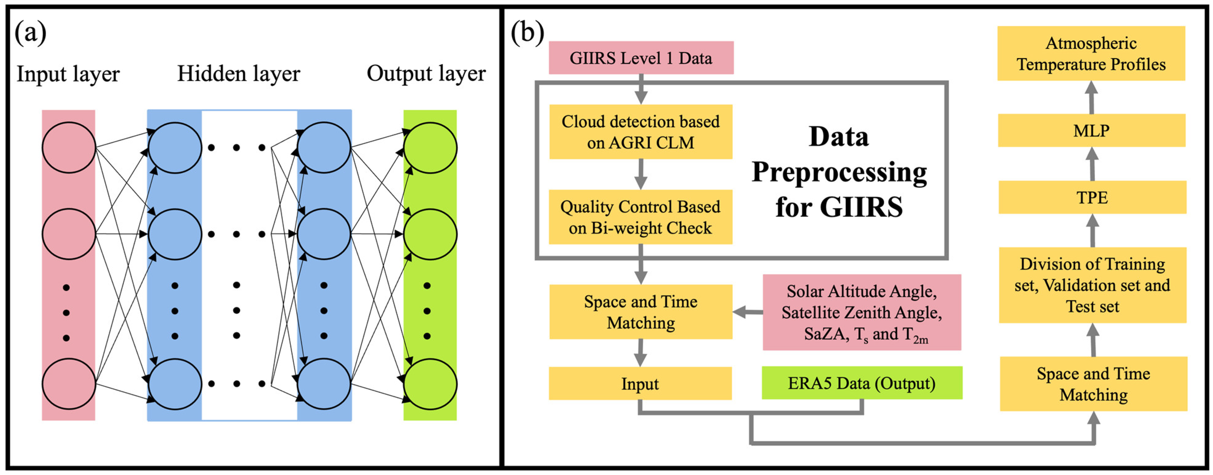
2.2.2. TPE-MLP Model
- (a)
- MLP
- (b)
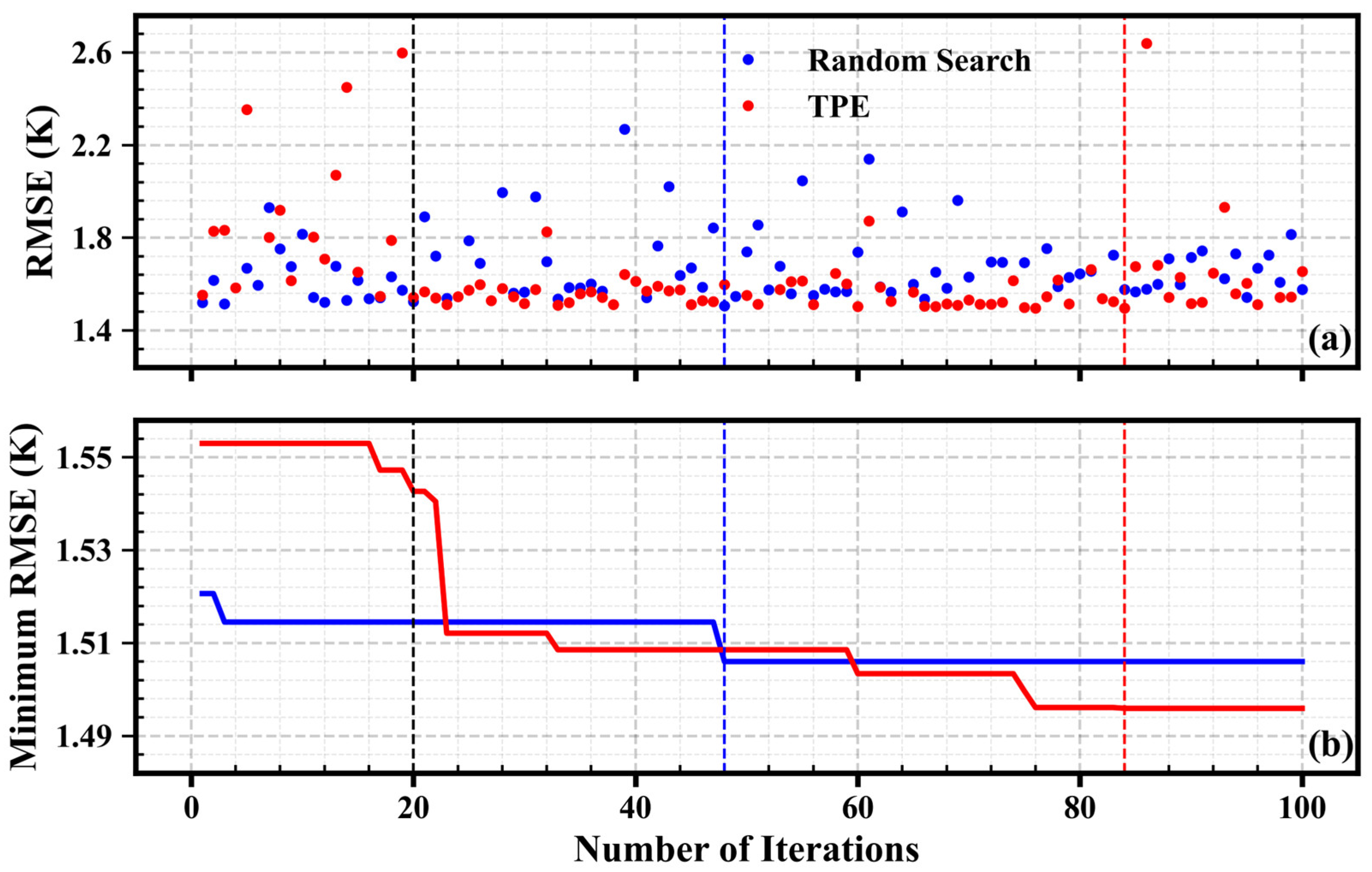
- Tree-structured Parzen Estimator (TPE)
| Algorithm 1. Tree-structured Parzen Estimator (TPE) |
| 1: Generate by random searching. 2: While do 3: Divide 4: Compute by adding the likelihood probability distribution of all points included in each group. 5: Generate several candidates 6: Set 7: Evaluate 8: Update 9: end while 10: Find 11: Return |
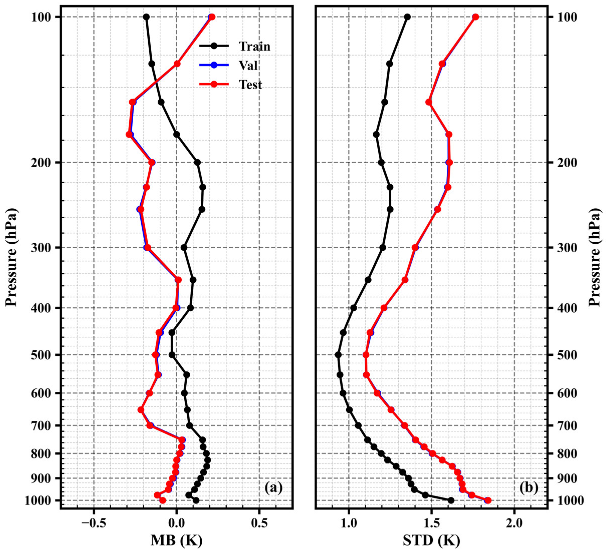
2.2.3. Process of TPE-MLP Model
2.2.4. Evaluation Methods
3. Results
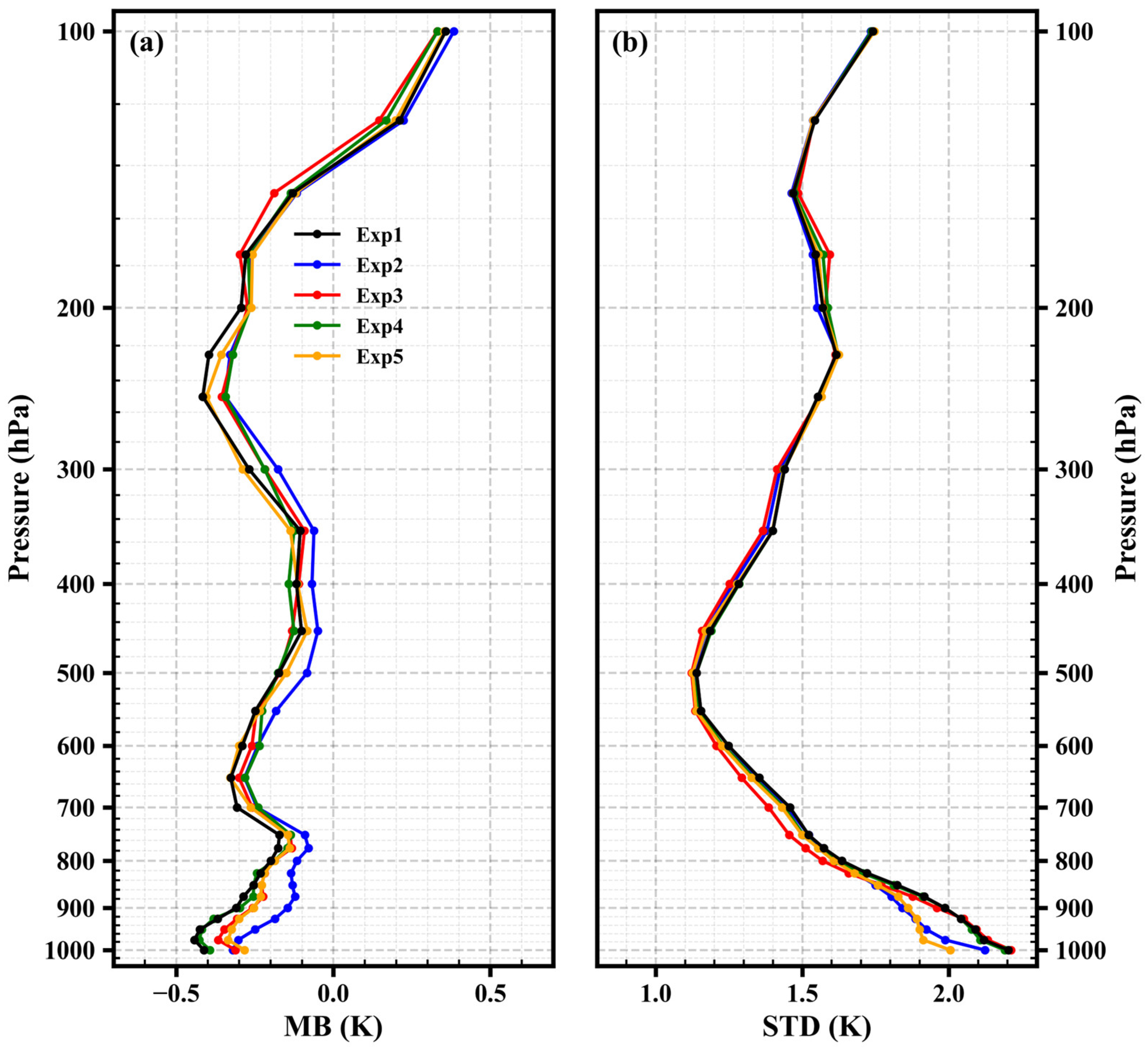
3.1. Sensitivity Experiments for the Input Layer
3.2. Hyper-Parameter Optimization
3.3. Analysis of Influencing Factors
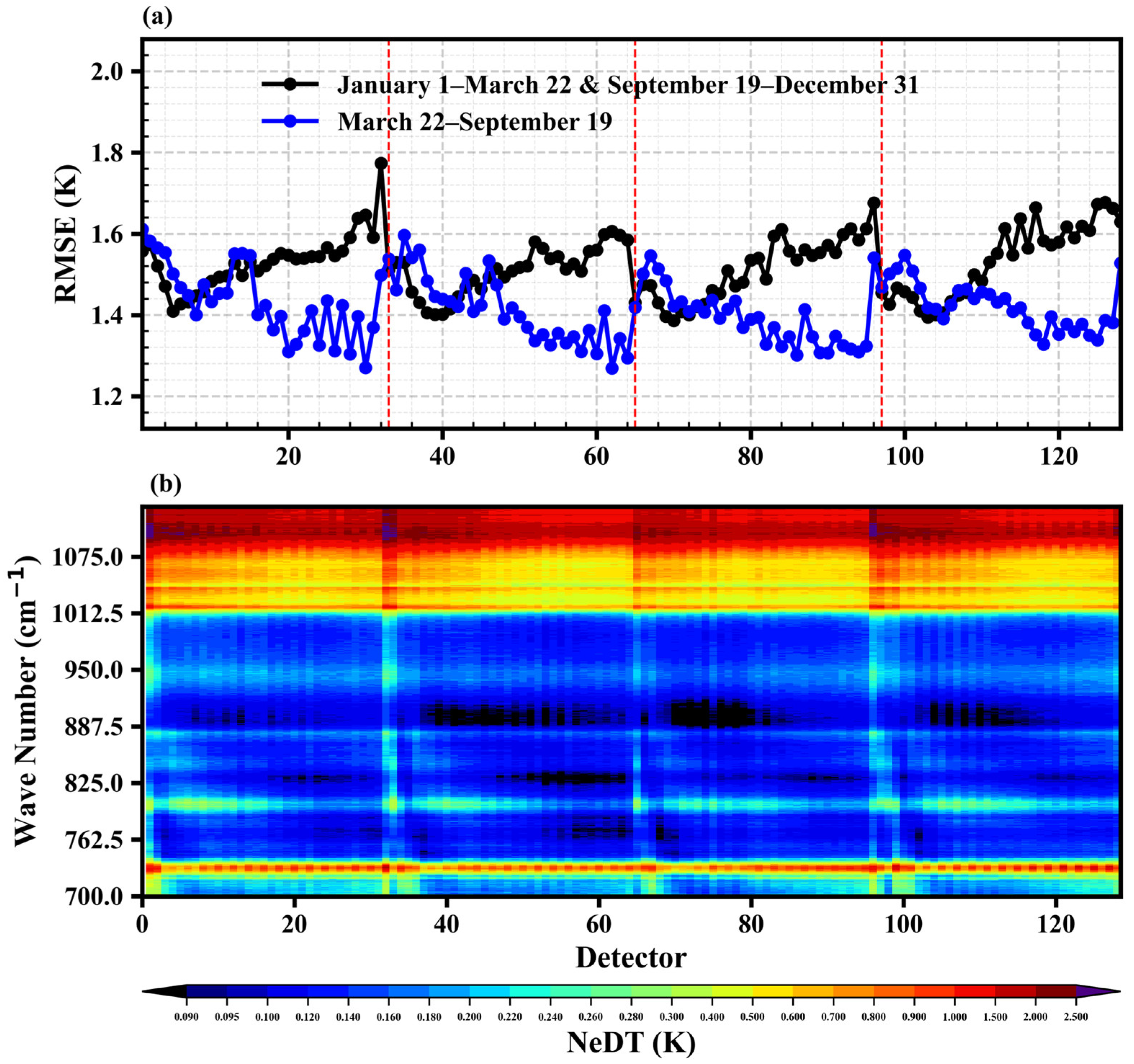
3.3.1. Variation with Detectors
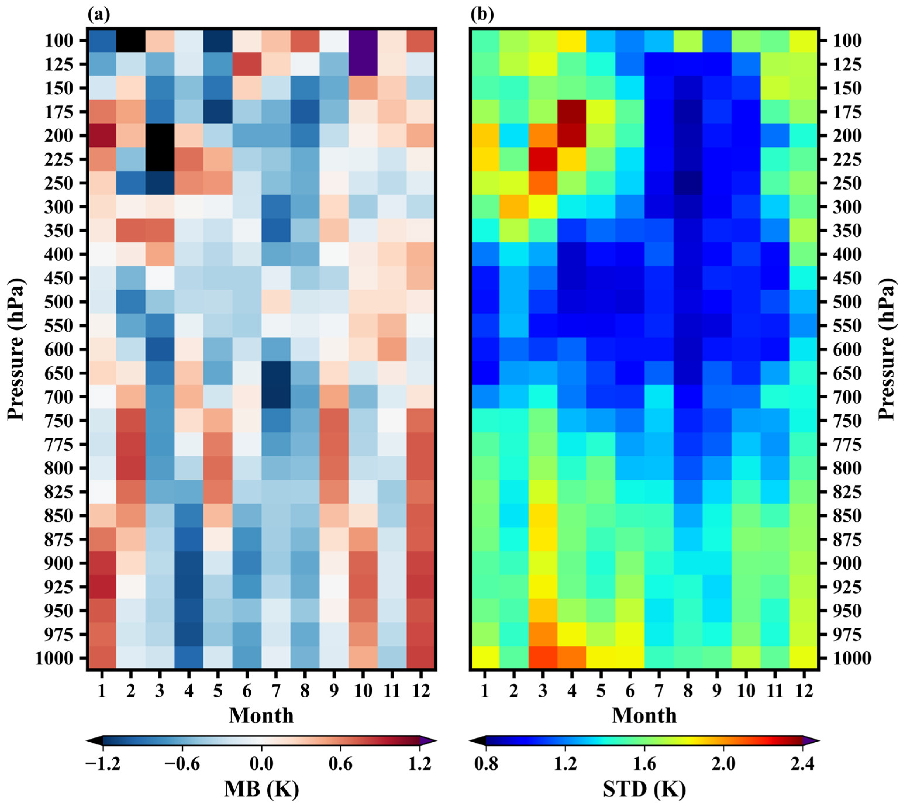
3.3.2. Monthly Variation
3.3.3. Diurnal Variation
3.4. Comparison between Retrieved Temperature Profiles and In Situ Sounding Data
4. Discussion
Supplementary Materials
Author Contributions
Funding
Data Availability Statement
Acknowledgments
Conflicts of Interest
References
- Eyre, J.R.; Bell, W.; Cotton, J.; English, S.J.; Forsythe, M.; Healy, S.B.; Pavelin, E.G. Assimilation of Satellite Data in Numerical Weather Prediction. Part II: Recent Years. Q. J. R. Meteorol. Soc. 2022, 148, 521–556. [Google Scholar] [CrossRef]
- Menzel, W.P.; Schmit, T.J.; Zhang, P.; Li, J. Satellite-Based Atmospheric Infrared Sounder Development and Applications. Bull. Am. Meteorol. Soc. 2018, 99, 583–603. [Google Scholar] [CrossRef]
- Guan, Y.; Ren, J.; Bao, Y.; Lu, Q.; Liu, H.; Xiao, X. Research of the Infrared High Spectral (IASI) Satellite Remote Sensing Atmospheric Temperature and Humidity Profiles Based on the One-Dimensional Variational Algorithm. Trans. Atmos. Sci. 2019, 42, 602–611. [Google Scholar] [CrossRef]
- Huang, P.; Guo, Q.; Han, C.; Zhang, C.; Yang, T.; Huang, S. An Improved Method Combining ANN and 1D-Var for the Retrieval of Atmospheric Temperature Profiles from FY-4A/GIIRS Hyperspectral Data. Remote Sens. 2021, 13, 481. [Google Scholar] [CrossRef]
- Sieglaff, J.M.; Schmit, T.J.; Menzel, W.P.; Ackerman, S.A. Inferring Convective Weather Characteristics with Geostationary High Spectral Resolution IR Window Measurements: A Look into the Future. J. Atmos. Ocean. Technol. 2009, 26, 1527–1541. [Google Scholar] [CrossRef]
- Iturbide-Sanchez, F.; Wang, Z.; Kalluri, S.; Chen, Y.; Lynch, E.; Divakarla, M.; Tan, C.; Zhu, T.; Cao, C. Exploration of a Future NOAA Infrared Sounder in Geostationary Earth Orbit. IEEE J. Sel. Top. Appl. Earth Obs. Remote Sens. 2022, 15, 1543–1561. [Google Scholar] [CrossRef]
- Collard, A.D.; McNally, A.P. The Assimilation of Infrared Atmospheric Sounding Interferometer Radiances at ECMWF. Q. J. R. Meteorol. Soc. 2009, 135, 1044–1058. [Google Scholar] [CrossRef]
- Eresmaa, R.; Letertre-Danczak, J.; Lupu, C.; Bormann, N.; McNally, A.P. The Assimilation of Cross-track Infrared Sounder Radiances at ECMWF. Q. J. R. Meteorol. Soc. 2017, 143, 3177–3188. [Google Scholar] [CrossRef]
- Aumann, H.H.; Chahine, M.T.; Gautier, C.; Goldberg, M.D.; Kalnay, E.; McMillin, L.M.; Revercomb, H.; Rosenkranz, P.W.; Smith, W.L.; Staelin, D.H.; et al. AIRS/AMSU/HSB on the Aqua Mission: Design, Science Objectives, Data Products, and Processing Systems. IEEE Trans. Geosci. Remote Sens. 2003, 41, 253–264. [Google Scholar] [CrossRef]
- Cayla, F.; Javelle, P. IASI: Instrument Overview. In Proceedings of the Infrared Spaceborne Remote Sensing III; SPIE: Bellingham, WA, USA, 1995; Volume 2553, pp. 316–328. [Google Scholar]
- Glumb, R.J.; Jordan, D.C.; Mantica, P. Development of the Crosstrack Infrared Sounder (CrIS) Sensor Design. In Proceedings of the Infrared Spaceborne Remote Sensing IX; SPIE: Bellingham, WA, USA, 2002; Volume 4486, pp. 411–424. [Google Scholar]
- Li, J.; Menzel, W.P.; Schmit, T.J.; Schmetz, J. Applications of Geostationary Hyperspectral Infrared Sounder Observations: Progress, Challenges, and Future Perspectives. Bull. Am. Meteorol. Soc. 2022, 103, E2733–E2755. [Google Scholar] [CrossRef]
- Chen, R.; Gao, C.; Wu, X.; Zhou, S.; Hua, J.; Ding, L. Application of FY-4 Atmospheric Vertical Sounder in Weather Forecast. J. Infrared Millim. Waves 2019, 38, 285–289. [Google Scholar] [CrossRef]
- Ma, Z.; Li, J.; Han, W.; Li, Z.; Zeng, Q.; Menzel, W.P.; Schmit, T.J.; Di, D.; Liu, C. Four-Dimensional Wind Fields from Geostationary Hyperspectral Infrared Sounder Radiance Measurements with High Temporal Resolution. Geophys. Res. Lett. 2021, 48, e2021GL093794. [Google Scholar] [CrossRef]
- Maier, J.; Knuteson, R. Data Fusion of GEO FY-4A GIIRS and LEO Hyperspectral Infrared Sounders with Surface Observations: A Hong Kong Case Study. J. Atmos. Ocean. Technol. 2022, 39, 259–270. [Google Scholar] [CrossRef]
- Schmit, T.J.; Li, J.; Ackerman, S.A.; Gurka, J.J. High-Spectral- and High-Temporal-Resolution Infrared Measurements from Geostationary Orbit. J. Atmos. Ocean. Technol. 2009, 26, 2273–2292. [Google Scholar] [CrossRef]
- Guo, Q.; Yang, J.; Wei, C.; Chen, B.; Wang, X.; Han, C.; Hui, W.; Xu, W.; Wen, R.; Liu, Y. Spectrum Calibration of the First Hyperspectral Infrared Measurements from a Geostationary Platform: Method and Preliminary Assessment. Q. J. R. Meteorolog. Soc. 2021, 147, 1562–1583. [Google Scholar] [CrossRef]
- Yang, J.; Zhang, Z.; Wei, C.; Lu, F.; Guo, Q. Introducing the New Generation of Chinese Geostationary Weather Satellites, Fengyun-4. Bull. Am. Meteorol. Soc. 2017, 98, 1637–1658. [Google Scholar] [CrossRef]
- Yin, R.; Han, W.; Gao, Z.; Di, D. The Evaluation of FY4A ’s Geostationary Interferometric Infrared Sounder (GIIRS) Long-wave Temperature Sounding Channels Using the GRAPES Global 4D-Var. Q. J. R. Meteorol. Soc. 2020, 146, 1459–1476. [Google Scholar] [CrossRef]
- Smith, W.; Woolf, H.; Jacob, W. A Regression Method for Obtaining Real-Time Temperature and Geopotential Height Profiles from Satellite Spectrometer Measurements and Its Application to Nimbus 3 “SIRS” Observations. Mon. Weather Rev. 1970, 98, 582–603. [Google Scholar] [CrossRef]
- Smith, W.; Woolf, H. The Use of Eigenvectors of Statistical Covariance Matrices for Interpreting Satellite Sounding Radiometer Observations. J. Atmos. Sci. 1976, 33, 1127–1140. [Google Scholar] [CrossRef]
- Chedin, A.; Scott, N.; Wahiche, C.; Moulinier, P. The Improved Initialization Inversion Method: A High Resolution Physical Method for Temperature Retrievals from Satellites of the TIROS-N Series. J. Appl. Meteorol. Clim. 1985, 24, 128–143. [Google Scholar] [CrossRef]
- Smith, W.; Woolf, H.; Hayden, C.; Schreiner, A. The Simultaneous Export Retrieval Package. In Proceedings of the Technical Proceedings of the Second International TOVS Study Conference, Iglis, Austria, 18–22 February 1985; Cooperative Institute for Meteorological Satellite Studies, University of Wisconsin–Madison: Madison, WI, USA, 1985; pp. 224–253. [Google Scholar]
- Susskind, J.; Rosenfield, J.; Reuter, D.; Chahine, M.T. Remote Sensing of Weather and Climate Parameters from HIRS2/MSU on TIROS-N. J. Geophys. Res. 1984, 89, 4677. [Google Scholar] [CrossRef]
- Milstein, A.B.; Blackwell, W.J. Neural Network Temperature and Moisture Retrieval Algorithm Validation for AIRS/AMSU and CrIS/ATMS. J. Geophys. Res. Atmos. 2016, 121, 1414–1430. [Google Scholar] [CrossRef]
- Berndt, E.; Smith, N.; Burks, J.; White, K.; Esmaili, R.; Kuciauskas, A.; Duran, E.; Allen, R.; LaFontaine, F.; Szkodzinski, J. Gridded Satellite Sounding Retrievals in Operational Weather Forecasting: Product Description and Emerging Applications. Remote Sens. 2020, 12, 3311. [Google Scholar] [CrossRef]
- Berndt, E.B.; Smith, N.; Barnet, C.D. Integrating NASA Aqua AIRS in a Real-Time NUCAPS Science-to-Applications System to Support Severe Weather Forecasting. Earth Space Sci. 2023, 10, e2022EA002725. [Google Scholar] [CrossRef]
- Kahn, B.H.; Berndt, E.B.; Case, J.L.; Kalmus, P.M.; Richardson, M.T. A Nowcasting Approach for Low-Earth-Orbiting Hyperspectral Infrared Soundings within the Convective Environment. Weather Forecast 2023, 38, 1295–1312. [Google Scholar] [CrossRef]
- Kalmus, P.; Kahn, B.H.; Freeman, S.W.; Van Den Heever, S.C. Trajectory-Enhanced AIRS Observations of Environmental Factors Driving Severe Convective Storms. Mon. Weather Rev. 2019, 147, 1633–1653. [Google Scholar] [CrossRef]
- Li, J.; Li, J.; Otkin, J.; Schmit, T.J.; Liu, C.-Y. Warning Information in a Preconvection Environment from the Geostationary Advanced Infrared Sounding System—A Simulation Study Using the IHOP Case. J. Appl. Meteorol. Clim. 2011, 50, 776–783. [Google Scholar] [CrossRef]
- Smith, W.L.; Weisz, E.; Kireev, S.V.; Zhou, D.K.; Li, Z.; Borbas, E.E. Dual-Regression Retrieval Algorithm for Real-Time Processing of Satellite Ultraspectral Radiances. J. Appl. Meteorol. Clim. 2012, 51, 1455–1476. [Google Scholar] [CrossRef]
- Li, J.; Zeng, Q. Infrared Remote Sensing of Clear Atmosphere and Related Inversion Problem. Part II: Experimental Study. Chin. J. Atmos. Sci. 1997, 21, 214–222. [Google Scholar] [CrossRef]
- Zhang, J.; Li, Z.; Li, J.; Li, J. Ensemble Retrieval of Atmospheric Temperature Profiles from AIRS. Adv. Atmos. Sci. 2014, 31, 559–569. [Google Scholar] [CrossRef]
- Susskind, J.; Blaisdell, J.M.; Iredell, L.; Keita, F. Improved Temperature Sounding and Quality Control Methodology Using AIRS/AMSU Data: The AIRS Science Team Version 5 Retrieval Algorithm. IEEE Trans. Geosci. Remote Sens. 2011, 49, 883–907. [Google Scholar] [CrossRef]
- Susskind, J.; Barnet, C.; Blaisdell, J.; Iredell, L.; Keita, F.; Kouvaris, L.; Molnar, G.; Chahine, M. Accuracy of Geophysical Parameters Derived from Atmospheric Infrared Sounder/Advanced Microwave Sounding Unit as a Function of Fractional Cloud Cover. J. Geophys. Res. 2006, 111, 2005JD006272. [Google Scholar] [CrossRef]
- Xue, Q.; Guan, L.; Shi, X. One-Dimensional Variational Retrieval of Temperature and Humidity Profiles from the FY4A GIIRS. Adv. Atmos. Sci. 2022, 39, 471–486. [Google Scholar] [CrossRef]
- Susskind, J.; Bamet, C.; Blaisdell, J. Determination of Atmospheric and Surface Parameters from Simulated AIRS/AMSU/HSB Sounding Data: Retrieval and Cloud Clearing Methodology. Adv. Space Res. 1998, 21, 369–384. [Google Scholar] [CrossRef]
- Nalli, N.R.; Barnet, C.D.; Reale, A.; Tobin, D.; Gambacorta, A.; Maddy, E.S.; Joseph, E.; Sun, B.; Borg, L.; Mollner, A.K.; et al. Validation of Satellite Sounder Environmental Data Records: Application to the Cross-track Infrared Microwave Sounder Suite. J. Geophys. Res. Atmos. 2013, 118, 13,628–13,643. [Google Scholar] [CrossRef]
- Jiang, D.; Cao, S.; Qu, Y. Preliminary Study on the Capacity of High Spectral Resolution Infrared Atmospheric Sounding Instrument Using AIRS Measurements. J. Trop. Meteorol. 2010, 26, 819–824. [Google Scholar] [CrossRef]
- Cai, X.; Bao, Y.; Petropoulos, G.P.; Lu, F.; Lu, Q.; Zhu, L.; Wu, Y. Temperature and Humidity Profile Retrieval from FY4-GIIRS Hyperspectral Data Using Artificial Neural Networks. Remote Sens. 2020, 12, 1872. [Google Scholar] [CrossRef]
- Cao, X.; Li, X.; Luo, Q.; Liu, S.; Li, P.; Liu, X. Review of Temperature Profile Inversion of Satellite-Borne Infrared Hyperspectral Sensors. Natl. Remote Sens. Bull. 2021, 25, 577–589. [Google Scholar] [CrossRef]
- Zhao, Y.; Zhou, D.; Yan, H. An Improved Retrieval Method of Atmospheric Parameter Profiles Based on the BP Neural Network. Atmos. Res. 2018, 213, 389–397. [Google Scholar] [CrossRef]
- Snoek, J.; Larochelle, H.; Adams, R.P. Practical Bayesian Optimization of Machine Learning Algorithms. Adv. Neural Inf. Process. Syst. 2012, 25. [Google Scholar] [CrossRef]
- Bao, Y.; Wang, Z.; Chen, Q.; Zhou, A.; Dong, Y.; Min, J. Preliminary Study on Atmospheric Temperature Profiles Retrieval from GIIRS Based on FY-4A Satelite. Aerosp. Shanghai 2017, 34, 28–37. [Google Scholar] [CrossRef]
- Bergstra, J.; Bengio, Y. Random Search for Hyper-Parameter Optimization. J. Mach. Learn. Res. 2012, 13, 281–305. [Google Scholar]
- Jo, Y.; Min, K.; Jung, D.; Sunwoo, M.; Han, M. Comparative Study of the Artificial Neural Network with Three Hyper-Parameter Optimization Methods for the Precise LP-EGR Estimation Using in-Cylinder Pressure in a Turbocharged GDI Engine. Appl. Therm. Eng. 2019, 149, 1324–1334. [Google Scholar] [CrossRef]
- Bergstra, J.; Bardenet, R.; Bengio, Y.; Kégl, B. Algorithms for Hyper-Parameter Optimization. Adv. Neural Inf. Process. Syst. 2011, 24, 2546–2554. [Google Scholar]
- Pan, L.; Lü, D. A New Method for Retrieving Equivalent Cloud Base Height and Equivalent Emissivity by Using the Ground-Based Atmospheric Emitted Radiance Interferometer (AERI). Sci. China Earth Sci. 2013, 56, 43–53. [Google Scholar] [CrossRef]
- Min, M.; Wu, C.; Li, C.; Liu, H.; Xu, N.; Wu, X.; Chen, L.; Wang, F.; Sun, F.; Qin, D.; et al. Developing the Science Product Algorithm Testbed for Chinese Next-Generation Geostationary Meteorological Satellites: Fengyun-4 Series. J. Meteorol. Res. 2017, 31, 708–719. [Google Scholar] [CrossRef]
- Corner, B.R.; Palmer, R.D.; Larsen, M.F. A New Radiosonde System for Profiling the Lower Troposphere. J. Atmos. Ocean. Technol. 1999, 16, 828–836. [Google Scholar] [CrossRef]
- Lanzante, J.R. Resistant, Robust and Non-Parametric Techniques for the Analysis of Climate Data: Theory and Examples, Including Applications to Historical Radiosonde Station Data. Int. J. Climatol. 1996, 16, 1197–1226. [Google Scholar] [CrossRef]
- Mapes, B.E.; Ciesielski, P.E.; Johnson, R.H. Sampling Errors in Rawinsonde-Array Budgets. J. Atmos. Sci. 2003, 60, 2697–2714. [Google Scholar] [CrossRef]
- Miloshevich, L.M.; Vömel, H.; Paukkunen, A.; Heymsfield, A.J.; Oltmans, S.J. Characterization and Correction of Relative Humidity Measurements from Vaisala RS80-A Radiosondes at Cold Temperatures. J. Atmos. Ocean. Technol. 2001, 18, 135–156. [Google Scholar] [CrossRef]
- Susskind, J.; Barnet, C.D.; Blaisdell, J.M. Retrieval of Atmospheric and Surface Parameters from AIRS/AMSU/HSB Data in the Presence of Clouds. IEEE Trans. Geosci. Remote Sens. 2003, 41, 390–409. [Google Scholar] [CrossRef]
- Zou, X.; Zeng, Z. A Quality Control Procedure for GPS Radio Occultation Data. J. Geophys. Res. 2006, 111, D02112. [Google Scholar] [CrossRef]
- Barber, C.B.; Dobkin, D.P.; Huhdanpaa, H. The Quickhull Algorithm for Convex Hulls. ACM Trans. Math. Softw. 1996, 22, 469–483. [Google Scholar] [CrossRef]
- Kingma, D.P.; Ba, J. Adam: A Method for Stochastic Optimization. arXiv 2017, arXiv:1412.6980. [Google Scholar] [CrossRef]
- Du, M.; Cui, L.; Lu, F.; Peng, J.; Shi, J.; Liu, D.; Fan, H. Quality evaluation of FY-4A/GIIRS atmospheric temperature profile. J. Infrared Millim. Waves 2023, 42, 399–409. [Google Scholar] [CrossRef]
- Borbas, E.E.; Menzel, W.P.; Weisz, E.; Devenyi, D. Deriving Atmospheric Temperature of the Tropopause Region–Upper Troposphere by Combining Information from GPS Radio Occultation Refractivity and High-Spectral-Resolution Infrared Radiance Measurements. J. Appl. Meteorol. Clim. 2008, 47, 2300–2310. [Google Scholar] [CrossRef]
- Borbás, É.; Menzel, W.P.; Li, J.; Woolf, H.M. Combining Radio Occultation Refractivities and IR/MW Radiances to Derive Temperature and Moisture Profiles: A Simulation Study plus Early Results Using CHAMP and ATOVS. J. Geophys. Res. 2003, 108, 2003JD003386. [Google Scholar] [CrossRef]


| Name | Formula |
|---|---|
| relu | |
| tanh | |
| sigmoid | |
| linear |
| Hyper-Parameters | Range of Values |
|---|---|
| Number of hidden layers | 1, 2, 3, 4, 5 |
| Number of neurons in hidden layer | 64 to 1024 at intervals of 64 |
| Learning rate | 1 × 10⁻², 1 × 10⁻³, 1 × 10⁻⁴ |
| Patience value | 2 to 20 at intervals of 2 |
| Activation function | relu, tanh, sigmoid |
| Batch size | 256 to 2560 at intervals of 256 |
| Experiment Names | Input of MLP |
|---|---|
| Exp1 | GIIRS |
| Exp2 | GIIRS + Solar Altitude Angle |
| Exp3 | GIIRS + Satellite Zenith Angle |
| Exp4 | GIIRS + Ts |
| Exp5 | GIIRS + T2m |
| Hyper-Parameters | Value |
|---|---|
| Number of hidden layers | 1 |
| Number of neurons in hidden layer | 832 |
| Learning rate | 1 × 10⁻⁴ |
| Patience value | 18 |
| Activation function | relu |
| Batch size | 256 |
Disclaimer/Publisher’s Note: The statements, opinions and data contained in all publications are solely those of the individual author(s) and contributor(s) and not of MDPI and/or the editor(s). MDPI and/or the editor(s) disclaim responsibility for any injury to people or property resulting from any ideas, methods, instructions or products referred to in the content. |
© 2024 by the authors. Licensee MDPI, Basel, Switzerland. This article is an open access article distributed under the terms and conditions of the Creative Commons Attribution (CC BY) license (https://creativecommons.org/licenses/by/4.0/).
Share and Cite
Xu, X.; Han, W.; Gao, Z.; Li, J.; Yin, R. Retrieval of Atmospheric Temperature Profiles from FY-4A/GIIRS Hyperspectral Data Based on TPE-MLP: Analysis of Retrieval Accuracy and Influencing Factors. Remote Sens. 2024, 16, 1976. https://doi.org/10.3390/rs16111976
Xu X, Han W, Gao Z, Li J, Yin R. Retrieval of Atmospheric Temperature Profiles from FY-4A/GIIRS Hyperspectral Data Based on TPE-MLP: Analysis of Retrieval Accuracy and Influencing Factors. Remote Sensing. 2024; 16(11):1976. https://doi.org/10.3390/rs16111976
Chicago/Turabian StyleXu, Xiaoze, Wei Han, Zhiqiu Gao, Jun Li, and Ruoying Yin. 2024. "Retrieval of Atmospheric Temperature Profiles from FY-4A/GIIRS Hyperspectral Data Based on TPE-MLP: Analysis of Retrieval Accuracy and Influencing Factors" Remote Sensing 16, no. 11: 1976. https://doi.org/10.3390/rs16111976