The Performance of Landsat-8 and Landsat-9 Data for Water Body Extraction Based on Various Water Indices: A Comparative Analysis

Abstract

The rapid and accurate extraction of water information from satellite imagery has been a crucial topic in remote sensing applications and has important value in water resources management, water environment monitoring, and disaster emergency management. Although the OLI-2 sensor onboard Landsat-9 is similar to the well-known OLI onboard Landsat-8, there were significant differences in the average absolute percentage change in the bands for water detection. Additionally, the performance of Landsat-9 in water body extraction is yet to be fully understood. Therefore, it is crucial to conduct comparative studies to evaluate the water extraction performance of Landsat-9 with Landsat-8. In this study, we analyze the performance of simultaneous Landsat-8 and Landsat-9 data for water body extraction based on eight common water indices (Normalized Difference Water Index (NDWI) and Modified Normalized Difference Water Index (MNDWI), Augmented Normalized Difference Water Index (ANDWI), Water Index 2015 (WI₂₀₁₅), tasseled cap wetness index (TCW), Automated Water Extraction Index for scenes with shadows (AWEI_sh) and without shadows (AWEI_nsh) and Multi-Band Water Index (MBWI)) to extract water bodies in seven study sites worldwide. The Otsu algorithm is utilized to automatically determine the optimal segmentation threshold for water body extraction. The results showed that (1) Landsat-9 satellite data can be used for water body extraction effectively, with results consistent with those from Landsat-8. The eight selected water indices in this study are applicable to both Landsat-8 and Landsat-9 satellites. (2) The NDWI index shows a larger variability in accuracy compared to other indices when used on Landsat-8 and Landsat-9 imagery. Therefore, additional caution should be exercised when using the NDWI for water body analysis with both Landsat-8 and Landsat-9 satellites simultaneously. (3) For Landsat-8 and Landsat-9 imagery, ratio-based water indices tend to have more omission errors, while difference-based indices are more prone to commission errors. Overall, ratio-based indices exhibit greater variability in overall accuracy, whereas difference-based indices demonstrate lower sensitivity to variations in the study area, showing smaller overall accuracy fluctuations and higher robustness. This study can provide necessary references for the selection of water indices based on the newest Landsat-9 data. The results are crucial for guiding the combined use of Landsat-8 and Landsat-9 for global surface water mapping and understanding its long-term changes.

1. Introduction

Surface water, a vital component of Earth’s environmental system, plays a significant role in supporting human productivity and providing immense environmental and ecological benefits [1,2]. However, the rapid and substantial fluctuations in these water bodies, driven by climatic change and human activities, have led to a series of detrimental water-related phenomena, including water scarcity, flooding, and pollution [3,4,5,6,7]. The importance of accurately identifying the dynamic changes in water bodies is undisputed. Correspondingly, it has emerged as an enduring research hotspot over recent decades [8,9]. This research theme not only aids in understanding and predicting the impacts of water body changes on the environment and society but also provides a framework for more effective management and protection of our water resources [10,11]. Therefore, it is of great significance to continue delving into this topic to better understand and manage global water resources.

Remote sensing technology offers a powerful tool for the large-scale, long-term monitoring of water bodies [1,12]. Its advantages include rapid, wide-area, and periodic imaging capabilities, which are invaluable for tracking dynamic changes in water bodies over time [13]. Several multispectral satellites have been extensively used for water body extraction. These include the Landsat series, MODIS, Sentinel-2, and Chinese Gaofen series [1,14,15,16,17]. These satellites provide rich spectral information, broad swath coverage, and short revisit periods, making them ideal for mapping large-scale surface water. Among these, the Landsat series satellites, launched by the United States for civilian land resource monitoring, has played a pivotal role in water body remote sensing research [18]. Their extensive temporal coverage, dating back to 1972 with the launch of Landsat-1 (also known as ERTS-1), have provided invaluable data for studying long-term changes in water bodies [19,20]. The latest addition to this series, Landsat-9, was launched in September 2021 as the successor to Landsat-8. The Operational Land Imager-2 (OLI-2) onboard Landsat-9 is largely identical to the Landsat-8 onboard OLI, offering calibrated imagery covering the solar-reflected wavelengths [21,22]. However, the performance of Landsat-9 in water body extraction is yet to be fully understood. Therefore, it is crucial to conduct comparative studies to evaluate the water extraction performance of Landsat-9 with its predecessor.

There exists a broad spectrum of methodologies designed for water body extraction based on medium-resolution optical satellite imagery [23,24]. These include pixel-level classification methods such as single-band thresholding segmentation, multi-band spectral relationship analysis, water index methods, and supervised classification methods (including popular machine learning and deep learning techniques) [10,25]. Object-level classification methods, such as object-based image analysis, are also employed [26]. Among these, the water index method stands out due to its simplicity and ease of use, making it a popular choice for large-scale or long-term water body extraction [27]. The water index method is grounded in the analysis of spectral characteristics of water bodies. It involves the selection of spectral bands closely associated with water body identification [28,29]. Through simple mathematical operations and the application of appropriate thresholds, this method facilitates the extraction of water body information. This approach leverages the unique spectral signatures of water bodies to distinguish them from other features in a landscape, providing a straightforward and effective means of water body extraction [30]. A variety of prominent water indices have been developed, including Normalized Difference Water Index (NDWI) [31], Modification of Normalized Difference Water Index (MNDWI) [32], Automated Water Extraction Index (AWEI) [28], Multi-Band Water Index (MBWI) [33], Water Index 2015 (WI₂₀₁₅) [34], Augmented Normalized Difference Water Index (ANDWI) [35] and Tasseled Cap Transformation (TCT) [36]. Existed publications have demonstrated their exceptional performance in water body extraction [1,5,16,37,38]. At present, whether at regional, national, or global scales, water body identification and mapping are inseparable from remote sensing water index methods. However, these indices were developed based on various existing remote sensing data, such as Landsat MSS, TM, ETM+, and OLI and other multi-spectral remotely sensed imagery. Therefore, it is crucial to analyze their applicability to new sensors, i.e., the OLI-2 sensor onboard Landsat-9.

The launch of the Landsat-9 satellite marks the start of a new era for the Landsat series. Compared to the Operational Land Imager (OLI) on Landsat-8, the OLI-2 on Landsat-9, while similar in terms of band configuration to its predecessor, has seen improvements in spectral response characterization and radiometric resolution [21,22]. Since the launch of Landsat-9, there have been some cross-comparisons of data from Landsat-8 and Landsat-9. Xu et al. [39] found that the surface reflectance data from Landsat-8 and Landsat-9 are almost consistent. However, there were significant differences in the average absolute percentage change in the bands for water detection [40,41]. It remains uncertain whether this deviation will be amplified in the calculation of water indices. This underscores the need for further research to fully understand the implications of these differences for water body extraction using Landsat-9 data. Consequently, it is urgent to conduct a systematic analysis of the performance of water body extraction based on Landsat-9 satellite imagery and a global comparison with the currently most widely used satellite in the Landsat series, i.e., Landsat-8. Our research aims to evaluate the differences between Landsat-9 and its predecessors, particularly in terms of water body extraction. This is crucial for assessing whether Landsat-9 can succeed Landsat-8 in continuing Earth observations, sensing global water resource dynamics, and supporting the achievement of sustainable development goals (SDGs).

Specifically, this study aims to compare the performance of multiple water indices for water extraction based on Landsat-8 and Landsat-9 datasets. Based on almost simultaneous Landsat-8 and Landsat-9 data, we employed eight common water indices to extract water bodies in seven study sites worldwide and further analyzed the application of water indices based on Landsat-9. This study aims to answer the following questions: (1) Are water indices applicable to Landsat-8 also applicable to Landsat-9? (2) Are there any differences in water extraction performance between Landsat-9 and Landsat-8? (3) Are Landsat-9 better in water extraction compared to Landsat-8? These results can guide our exploration of the capabilities and potential of the new Landsat-9 satellite in the field of remote sensing for water body extraction.

2. Study Areas and Data Source

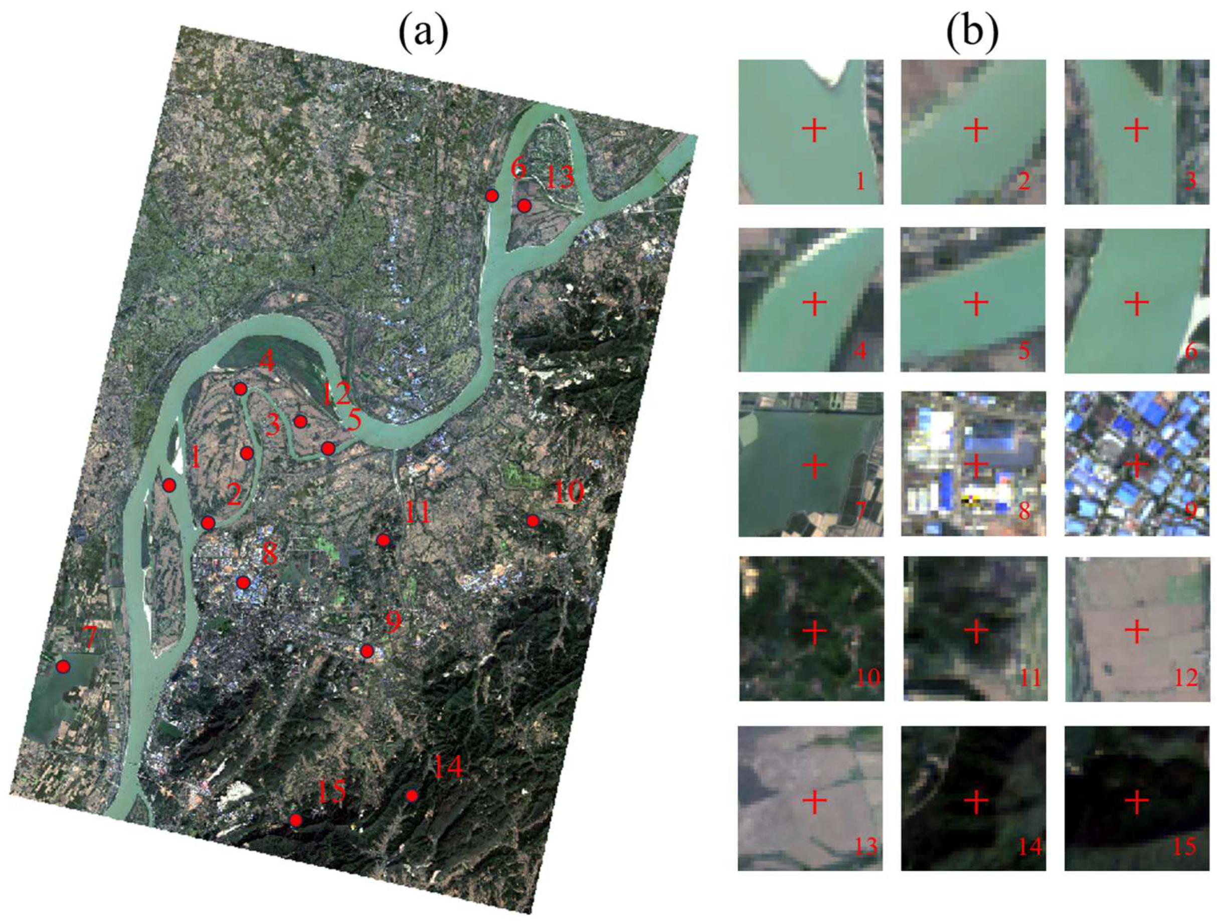
2.1. Study Area

To ensure a rigorous and representative comparative analysis, the variations in remote sensing image acquisition times, elevation, climate, terrain, vegetation cover types, and geological features were carefully considered. A total of seven test sites (Mille Lacs Lake, Lake Nipissing, the Tongling section of the Yangtze River, Lianhuan Lake, Sai Lake, Liangzi Lake, and Lake Wivenhoe) were selected (Figure 1). Various sites can enhance the diversity of the water body dataset and enable a robust validation of water index applications across varying geographical contexts.

Geographically, the selected areas span Asia, North America, and Oceania. Morphologically, the aquatic landscapes at these sites comprise a mixture of small ponds encircled by larger lakes, rivers of linear or irregular shapes, human-made reservoirs, and water channels in coastal zones. For the climatic features, these sites extend from coastal to inland settings, each characterized by unique climatic conditions, as detailed in

Table 1. Description of the seven test sites in this study.

No.	Names	Country	Climate	Water Type	Major Background Noise
1	Mille Lacs Lake	The United States of America	Temperate continental climate	Lake	Vegetation
2	Lake Nipissing	Canada	Temperate continental climate	Lake	Vegetation and Artificial building
3	Tongling section of Yangtze River	China	Temperate monsoon climate	River	Paddy field and Mountain shadow Wetland
4	Lianhuan Lake	China	Temperate monsoon climate	Lake cluster	Wetland
5	Sai Lake	China	Temperate monsoon climate	River and Lake	Artificial building
6	Liangzi Lake	China	Temperate monsoon climate	Lake	Artificial building
7	Lake Wivenhoe	Australia	Subtropical monsoon and humid climate	Artificial reservoir	Mountain shadow and Artificial building

.

2.2. Remote Sensing Data

In this study, data were utilized from both Landsat-8 OLI and Landsat-9 OLI-2 satellites. To minimize inter-dataset discrepancies and ensure accuracy in the extraction of aquatic information, it is crucial to acquire remote sensing images from both sensors, captured over the same area one day apart. Although Landsat-9 and Landsat-8 have an 8d temporal misalignment, making exact date-over-date comparisons infeasible, images from adjacent paths overlap within approximately 24 h. This overlap allows for the acquisition of nearly concurrent images. Accordingly, a total of fourteen sets of images from both Landsat-9 and Landsat-8, captured over the same scene and within a 24 h interval, were collected (

Table 2. Summary of the employed Landsat-8 OLI and Landsat-9 OLI-2 imagery and corresponding reference data in this study.

No.	Test Site	Path/Row	Acquisition Date	Data Source
1	Mille Lacs Lake	028/028	2022/08/31	Landsat-8 Collection 2 Level-2
		027/028	2022/09/01	Landsat-9 Collection 2 Level-2
2	Lake Nipissing	019/028	2023/09/04	Landsat-8 Collection 2 Level-2
		018 /028	2023/09/05	Landsat-9 Collection 2 Level-2
3	Tongling section of Yangtze River	120/039	2022/11/08	Landsat-8 Collection 2 Level-2
		121/038	2022/11/07	Landsat-9 Collection 2 Level-2
4	Lianhuan Lake	120/027	2022/11/08	Landsat-8 Collection 2 Level-2
		119/028	2022/11/09	Landsat-9 Collection 2 Level-2
5	Sai Lake	122/039	2022/08/18	Landsat-8 Collection 2 Level-2
		121/040	2022/08/19	Landsat-9 Collection 2 Level-2
6	Liangzi Lake	123/039	2022/05/05	Landsat-8 Collection 2 Level-2
		122/039	2022/05/06	Landsat-9 Collection 2 Level-2
7	Lake Wivenhoe	089/079	2022/10/29	Landsat-8 Collection 2 Level-2
		090/079	2022/10/28	Landsat-9 Collection 2 Level-2

).

All data were collected from the Google Earth Engine (GEE) platform (https://developers.google.cn/earth-engine (accessed on 12 May 2024)). The remote sensing image data primarily consisted of Tier 1 Level 2 Science Products (L2SP), which have undergone rigorous geometric correction based on ground control points, radiometric and atmospheric corrections, and solar zenith angle adjustments. These products feature a spatial resolution of 30 m. They can provide surface reflectance data that are ready for subsequent processing. More details of the employed data can be found at https://developers.google.cn/earth-engine/datasets/catalog/landsat (accessed on 12 May 2024). To further enhance image quality, the study employed image selection criteria on the GEE platform, prioritizing images with less than 20% cloud cover for subsequent analysis. After careful investigations, all the acquisition dates of employed satellite imagery were sunny clear-sky days, with no obvious precipitation in the previous and subsequent days. It is noted that the selection of imagery is a trade-off between the overlapping acquisition date and imagery quality.

3. Methodology

3.1. Water Index

In this study, various water indices were employed to enhance water body information for subsequent water extraction. To evaluate the applicability of these indices, the study categorized various water indices and selected representative ones to assess extraction accuracy and analyze the mechanisms influencing their performance. The effective extraction of water body information was facilitated by binarizing the index images via the appropriate threshold. This study incorporated eight water indices, including the commonly utilized Normalized Difference Water Index (NDWI) and Modified Normalized Difference Water Index (MNDWI), Augmented Normalized Difference Water Index (ANDWI), Water Index 2015 (WI₂₀₁₅), tasseled cap wetness index (TCW), automated water extraction index for scenes with shadows (AWEI_sh) and without shadows (AWEI_nsh), and Multi-Band Water Index (MBWI). The aim was to explore the differences in effectiveness and practicality of extracting surface water body information using Landsat-8 and Landsat-9 imagery. Detailed methodologies for calculating each water index, along with their respective sensor bases, are presented in

Table 3. Basic information of the employed water indices in this study.

Type	Water Index	Equation	Sensor	Reference
Ratio-based	NDWI	$(\mathrm{G}\mathrm{r}\mathrm{e}\mathrm{e}\mathrm{n}-\mathrm{N}\mathrm{I}\mathrm{R})/(\mathrm{G}\mathrm{r}\mathrm{e}\mathrm{e}\mathrm{n}+\mathrm{N}\mathrm{I}\mathrm{R})$	MSS	[31]
	MNDWI	$(\mathrm{G}\mathrm{r}\mathrm{e}\mathrm{e}\mathrm{n}-\mathrm{S}\mathrm{W}\mathrm{I}\mathrm{R}1)/(\mathrm{G}\mathrm{r}\mathrm{e}\mathrm{e}\mathrm{n}+\mathrm{S}\mathrm{W}\mathrm{I}\mathrm{R}1)$	TM	[32]
	ANDWI	$(\mathrm{B}\mathrm{l}\mathrm{u}\mathrm{e}+\mathrm{G}\mathrm{r}\mathrm{e}\mathrm{e}\mathrm{n}+\mathrm{R}\mathrm{e}\mathrm{d}-\mathrm{N}\mathrm{I}\mathrm{R}-\mathrm{S}\mathrm{W}\mathrm{I}\mathrm{R}1-\mathrm{S}\mathrm{W}\mathrm{I}\mathrm{R}2)/(\mathrm{B}\mathrm{l}\mathrm{u}\mathrm{e}+\mathrm{G}\mathrm{r}\mathrm{e}\mathrm{e}\mathrm{n}+\mathrm{R}\mathrm{e}\mathrm{d}+\mathrm{N}\mathrm{I}\mathrm{R}+\mathrm{S}\mathrm{W}\mathrm{I}\mathrm{R}1+\mathrm{S}\mathrm{W}\mathrm{I}\mathrm{R}2)$	ETM+/OLI	[35]
Difference-based	WI2015	$1.7204+171\times \mathrm{G}\mathrm{r}\mathrm{e}\mathrm{e}\mathrm{n}+3\times \mathrm{R}\mathrm{e}\mathrm{d}-70\times \mathrm{N}\mathrm{I}\mathrm{R}-45\times \mathrm{S}\mathrm{W}\mathrm{I}\mathrm{R}1-71\times \mathrm{S}\mathrm{W}\mathrm{I}\mathrm{R}2$	TM/ETM+/OLI	[34]
	TCW	$0.1446\times \mathrm{B}\mathrm{l}\mathrm{u}\mathrm{e}+0.1761\times \mathrm{G}\mathrm{r}\mathrm{e}\mathrm{e}\mathrm{n}+0.3322\times \mathrm{R}\mathrm{e}\mathrm{d}+0.3396\times \mathrm{N}\mathrm{I}\mathrm{R}-0.6210\times \mathrm{S}\mathrm{W}\mathrm{I}\mathrm{R}1-0.4186\times \mathrm{S}\mathrm{W}\mathrm{I}\mathrm{R}2-3.3828$	TM/ETM+	[36]
	AWEIsh	$\mathrm{B}\mathrm{l}\mathrm{u}\mathrm{e}+2.5\times \mathrm{G}\mathrm{r}\mathrm{e}\mathrm{e}\mathrm{n}-1.5\times (\mathrm{N}\mathrm{I}\mathrm{R}+\mathrm{S}\mathrm{W}\mathrm{I}\mathrm{R}1)-0.25\times \mathrm{S}\mathrm{W}\mathrm{I}\mathrm{R}2$	TM	[28]
	AWEInsh	$4\times (\mathrm{G}\mathrm{r}\mathrm{e}\mathrm{e}\mathrm{n}-\mathrm{S}\mathrm{W}\mathrm{I}\mathrm{R}1)-(0.25\times \mathrm{N}\mathrm{I}\mathrm{R}+2.75\times \mathrm{S}\mathrm{W}\mathrm{I}\mathrm{R}2)$	TM	[28]
	MBWI	$(2\times \mathrm{G}\mathrm{r}\mathrm{e}\mathrm{e}\mathrm{n})-\mathrm{R}\mathrm{e}\mathrm{d}-\mathrm{N}\mathrm{I}\mathrm{R}-\mathrm{S}\mathrm{W}\mathrm{I}\mathrm{R}1-\mathrm{S}\mathrm{W}\mathrm{I}\mathrm{R}2$	OLI	[33]

Note: Blue, Green, Red, NIR, SWIR1, and SWIR2 represent the surface reflectance of blue band, green band, red band, near-infrared band, and shortwave infrared band-1 and -2 in Landsat-8 and Landsat-9 imagery, respectively. MSS, TM, ETM+, and OLI represent the Landsat Multispectral Scanner, Thematic Mapper, Enhanced Thematic Mapper Plus, and Operational Land Imager (OLI) data, respectively.

.

3.2. Threshold Determination

The water body index can effectively enhance the class separability between water and non-water classes. On this basis, selecting an appropriate threshold to achieve the best possible separation effects is also the key to water mapping [13]. Consequently, a series of multi-modal density slicing methods were developed, such as Otsu, K-Means, Inter-modes, Maximum Entropy, Median, Concavity, Percentile, Inter-means, and Iterative Self-organizing Data Analysis (ISODATA) [42,43]. Among them, the Otsu algorithm is a typical adaptive thresholding technique for image segmentation, commonly used to convert grayscale images into binary images [44]. The fundamental advantage of the Otsu method lies in its ability to automatically select a threshold that divides the image into foreground and background, minimizing within-class variance and maximizing between-class variance.

The Otsu method is good at determining the best threshold automatically in a straightforward and effective way, which is particularly valuable in images with varying lighting conditions or contrast levels [45]. Compared to traditional methods that require manual threshold setting, the Otsu method significantly reduces subjectivity and the complexity of experimental operations [13]. In other words, this specific method is featured with satisfactory slicing effect and high efficiency. Although other advanced methods are also employed for threshold determination in water mapping, the Otsu method allows for keeping accuracy without sacrificing efficiency [12,46].

The application of Otsu’s method is suitable for the binarization of remote sensing water indices under bimodal distribution conditions [47]. Remote sensing images typically contain complex geographical and environmental information, with clear distinctions in gray levels between water and non-water regions in water index images [13]. The Otsu method effectively isolates water regions from these complex datasets by automatically identifying the optimal threshold based on the image’s statistical characteristics [25,48]. This capability is crucial for enhancing the accuracy and efficiency of water body extraction, especially in large-scale or automated water monitoring projects, thereby significantly improving processing speed and the reliability of results.

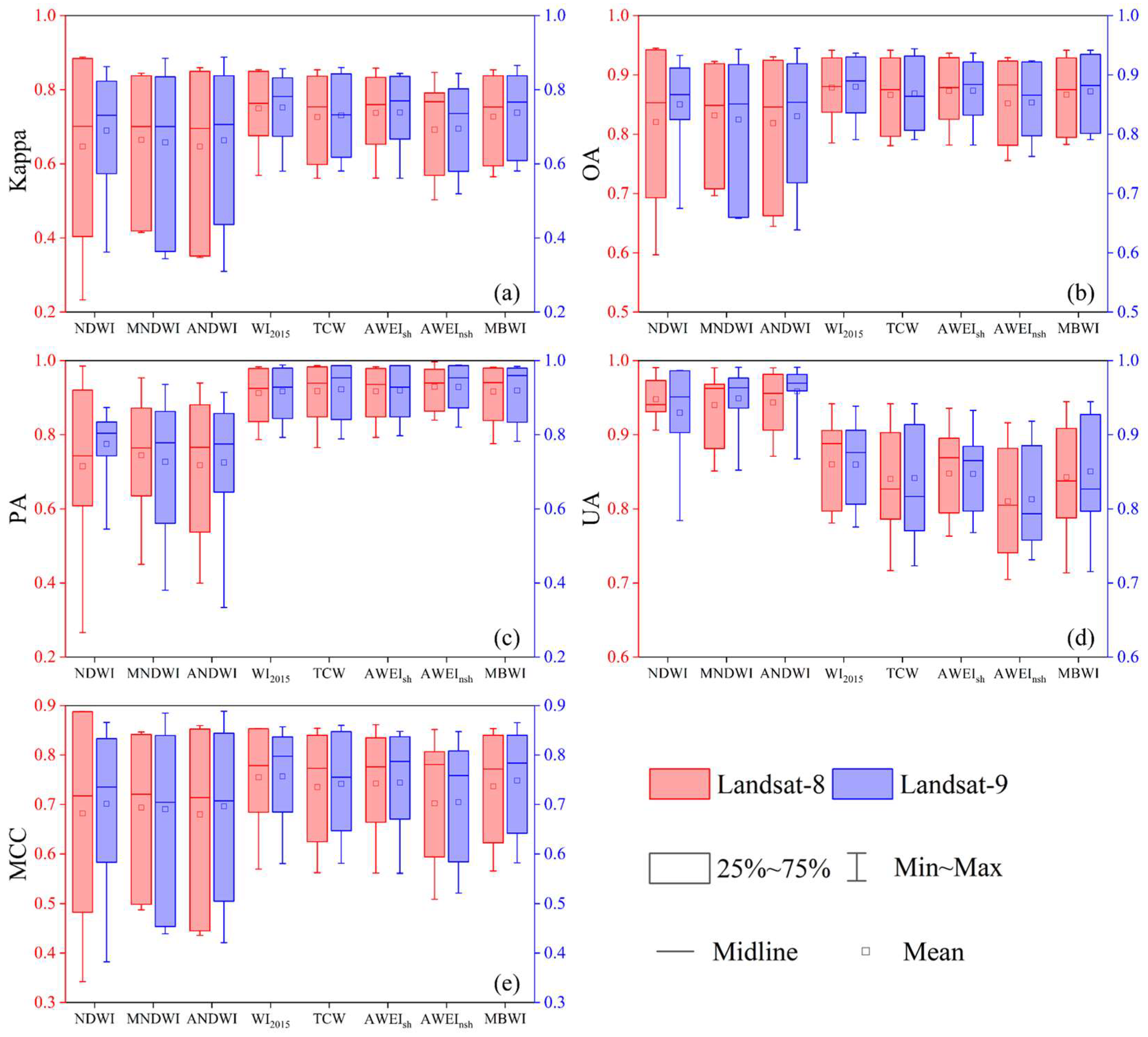
3.3. Accuracy Assessment

To comprehensively evaluate the classification accuracy of water indices, this study utilizes four key metrics: Overall Accuracy (OA), User Accuracy (UA), Producer Accuracy (PA), and the Kappa coefficient [49]. In addition, the Matthew Correlation coefficient (MCC) is also used for evaluating the extraction performance, which is particularly suited for unbalanced binary distributions [50]. MCC values range between −1 and 1, where a value of 1 represents a perfect classifier, whereas a value of 0 describes a classifier making random guesses [51]. These parameters are employed to analyze interpretative discrepancies across different test sites and to identify the spatial distribution of error-prone pixels.

In this study, validation data for the water and non-water samples were obtained through the visual interpretation of employed Landsat-8 and Landsat-9 imagery. For samples that are challenging to distinguish on 30 m Landsat imagery, we utilize high-resolution Google Earth and Chinese MapWorld imagery (<1 m) from similar time periods to assist in their identification. The satellite imagery utilized in this study was acquired during periods of sunny, clear skies, with no significant precipitation or flooding events. Moreover, the water extents in the seven test sites exhibited relative stability, showing minimum pixel changes over a short temporal span of 1 d, even in transitional areas. This consistency underscores the reliability of the data for accurate analysis and interpretation.

Additionally, these data were also used for extracting “pure” pixel samples from the same locations in both Landsat-8 and Landsat-9 imagery to provide a reference for the spectral differences between the two sets of images. Commonly, the ground area corresponding to a “pure” pixel contains only a single object (land cover type), and then the recorded information by this pixel (30 × 30 m corresponding to the pixel size of a 30 m-Landsat image) is the spectral characteristic of the pure object [33,52]. In this study, these points were randomly generated from the map and then manually confirmed to ensure the stable distribution of land cover types, including shadows, water, vegetation, and soil. The corresponding spectral features were used for analyzing the differences between both satellite images.

4. Results

4.1. Effects of Different Water Indices

To enhance the comparative analysis of the extraction performance of various water indices utilizing Landsat-9 OLI-2 data, this study systematically selected eight water indices. The effects of these indices were evaluated through a multi-dimensional framework, examining image discrepancies, correlations, and difference metrics.

4.1.1. Comparison of Different Water Indices in Landsat-9

Focusing on the Tongling section of the Yangtze River region, a total of eight water maps were generated (Figure 2). The visual analysis of the results from these water indices reveals that each index effectively enhances the contrast between aquatic and non-aquatic areas, clearly delineating the distribution of water bodies within the watershed.

The ratio-based indices NDWI, ANDWI, and MNDWI, as depicted in Figure 2b–d, exhibit significant and uniform distinctions between land and water areas, with NDWI showing the greatest difference (−0.827–0.983), resulting in a range of 1.810. In contrast, ANDWI shows a somewhat narrower range (ranging from −0.890 to 0.857), a difference of 1.747. The corresponding difference-based indices retain a considerable amount of surface detail, which is characteristic of these indices. Due to the inherent nature of difference-based indices, we did not conduct a comparative analysis of the highest and lowest values here. However, visually, the difference-based indices slightly lag behind the ratio-based indices, as they do not as effectively suppress information related to water fields. Overall, all eight water body indices we employed were capable of supporting subsequent analyses for water body extraction.

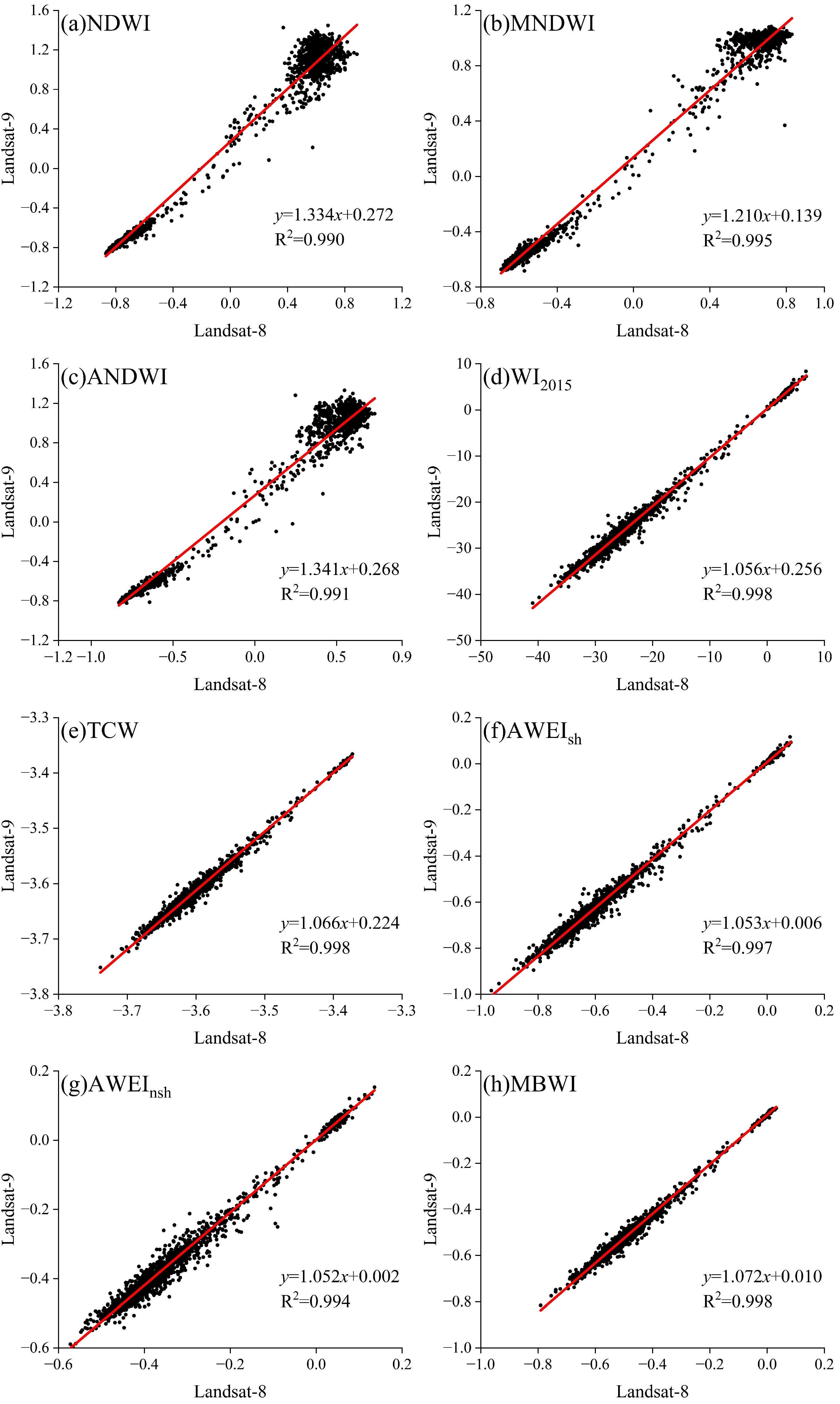
4.1.2. Differences of Seven Water Indices in Landsat-8 and Landsat-9

To better evaluate the differences between the water indices derived from Landsat-8 and Landsat-9 data, we examined the differences of index images (Landsat-8 scene minus Landsat-9 scene) from both satellites, focusing on the Lake Wivenhoe as illustrated in Figure 3. The differences are calculated by subtracting the index values derived from Landsat-8 data from those obtained using Landsat-9 data. In the water areas, differences are predominantly positive, indicating that the water indices calculated from Landsat-8 generally yield higher values than those from Landsat-9. For the terrestrial areas, the ratio-based indices (Figure 3a–c) tend to approach zero, indicating the minimal discrepancies between both datasets.

In the non-water areas, difference-based indices typically exhibit negative values, indicating that water indices calculated from Landsat-8 are generally lower than those derived from Landsat-9. As shown in Figure 3c, the difference in values between the two imagery indices of AWEI_sh is smaller compared to other indices. In Figure 3, it is obvious that most water regions appear lighter or near white, reflecting minimal disparities. The difference plot for AWEI_sh shows a maximum value of 0.509 and a minimum value of −0.477, with a total range of 0.986. Similar trends of small disparities in AWEI_sh index values are observed in other study areas, as detailed in Figures S1–S5.

However, the test site of Mille Lacs Lake (Figure 4) displays opposite characteristics to Lake Wivenhoe, with water indices predominantly showing negative differences. In non-water areas, the ratio-based water indices in both test sites tend to approach zero, while the difference-based indices display positive values, indicating that the majority of water index values calculated from Landsat-8 are greater than those from Landsat-9. More difference maps are shown in Figures S1–S5. These above results indicate that the performance of various water indices varies with geographical regions; however, there remains a strong consistency between Landsat-8 and Landsat-9 data across these areas.

4.1.3. Correlation among Various Water Indices

Based on the GEE platform, a total of 3000 data points were randomly selected for extracting the water index values in each pair of Landsat-8 and Landsat-9 imagery. Subsequently, a correlation analysis was conducted on the water indices calculated from two scenes within the Lake Wivenhoe area (Figure 5). Overall, both sets of data demonstrate high correlations across all eight indices, with R² values exceeding 0.990 for each. Notably, the highest correlations were observed in MBWI, TCW, and WI₂₀₁₅, all reaching an R² of 0.998, while the lowest was in NDWI (R² = 0.990). The graphical representation shows that the 3000 data points for all water body indices are predominantly positioned at the extremes of the fitted line. However, the distribution of ratio-based indices, especially NDWI, is more pronounced, with data points distinctly clustered at the extremes (Figure 5a). In contrast, TCW points are more densely concentrated at one end, associated with non-water body points. The R² values for MNDWI, NDWI, ANDWI, and AWEI_nsh are 0.995, 0.990, 0.991, and 0.994, respectively, indicating a slightly lower correlation compared to other indices. The additional correlation results are shown in Figures S6–S11.

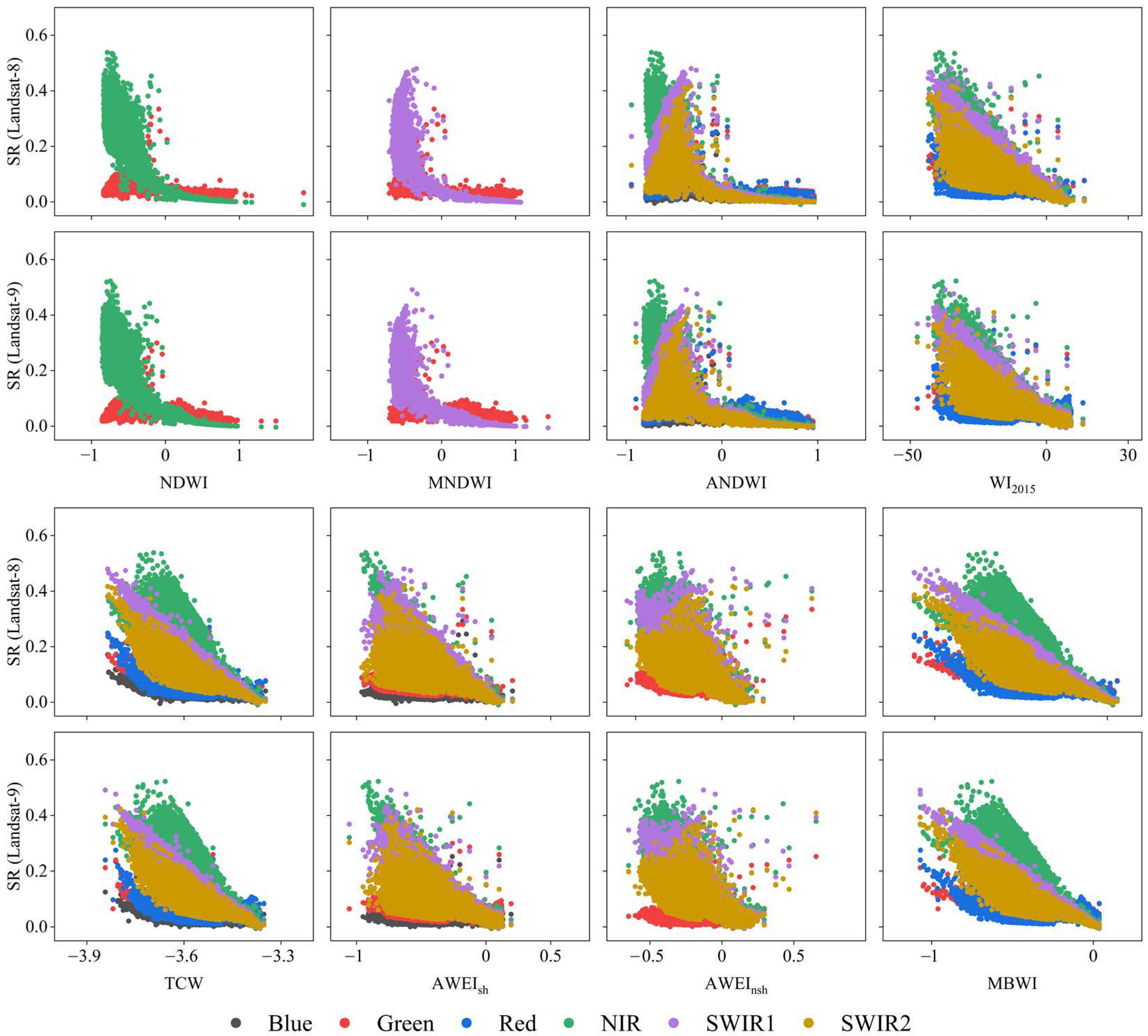
4.2. Separation of the Water Index

To assess the impact of spectral band differences on water extraction, the separability of water index values was analyzed within the Lake Wivenhoe region (Figure 6). The relationships between the indices and the corresponding spectral bands were also analyzed. Generally, there is consistency in the separability of water indices derived from both Landsat-8 and Landsat-9 data, with indices such as NDWI demonstrating identical reflectance distributions in the Green and NIR bands across both satellite images. However, indices like AWEI_nsh, AWEI_sh, and WI2015 show no distinct separation gaps, leading to significant uncertainty in their segmentation thresholds. Conversely, indices such as NDWI, MNDWI, MBWI, and ANDWI display clear gaps near zero, facilitating their direct application for water body segmentation across the entire study area based on established thresholds. As illustrated in Figure 6, the division of water bodies using NDWI and MNDWI is predominantly determined by the greater reflectance values in the Green band compared to the NIR and SWIR1 bands. In the other test sites, the separations of the water index are similar (Figures S12–S17).

For the threshold, histograms were generated using Lake Wivenhoe as a case study (Figure 7). Eight different water indices were utilized, all designed to suppress the differences in surface reflectance between water and non-water bodies, resulting in more concentrated pixel values ranging from −1 to 1 for indices like NDWI. These indices amplify the distinction between water and non-water areas. Typically, the histogram of a water index image displays two peaks, with the right peak representing water areas, as seen in the WI₂₀₁₅ index image, and the left peak representing non-water areas.

As shown in Figure 7, it is evident that although some water peaks are quite low due to the small proportion of water in the study area, both Landsat-8 and Landsat-9 exhibit similar morphologies, with most images showing a bimodal distribution. This characteristic makes it straightforward to distinctly differentiate between the index values of water and non-water bodies. The ratio-based indices, such as NDWI, MNDWI, and ANDWI, feature a large separation between the two peaks, where water (right peak) and non-water (left peak) are far apart and do not overlap. This clear separation facilitates the setting of thresholds for water body segmentation. Conversely, the difference-based indices like AWEI_nsh and MBWI (Figure 7g,h) show a shorter distance between peaks, resulting in minimal separation.

In this specific test site, the thresholds for ratio-based water indices differ significantly between Landsat-8 and Landsat-9 imagery (Figure 7a–c). For example, the Otsu threshold for the NDWI index is 0.005 on Landsat-8 images and −0.095 on Landsat-9 images, a difference of 0.100. In contrast, the thresholds for difference-based indices show smaller discrepancies; the MBWI index has an Otsu threshold of −0.285 on Landsat-8 images and −0.275 on Landsat-9 images, with a minimal difference of 0.010.

Overall, the histograms of the index images from Landsat-8 and Landsat-9 are consistent (Figure 7 and Figures S18–S23). The ratio-based indices, being greater than 0, demonstrate a distinct difference in the crest of the water peak between the two satellite images; hence, the threshold for ratio-based indices exhibits more variability between Landsat-8 and Landsat-9 imagery.

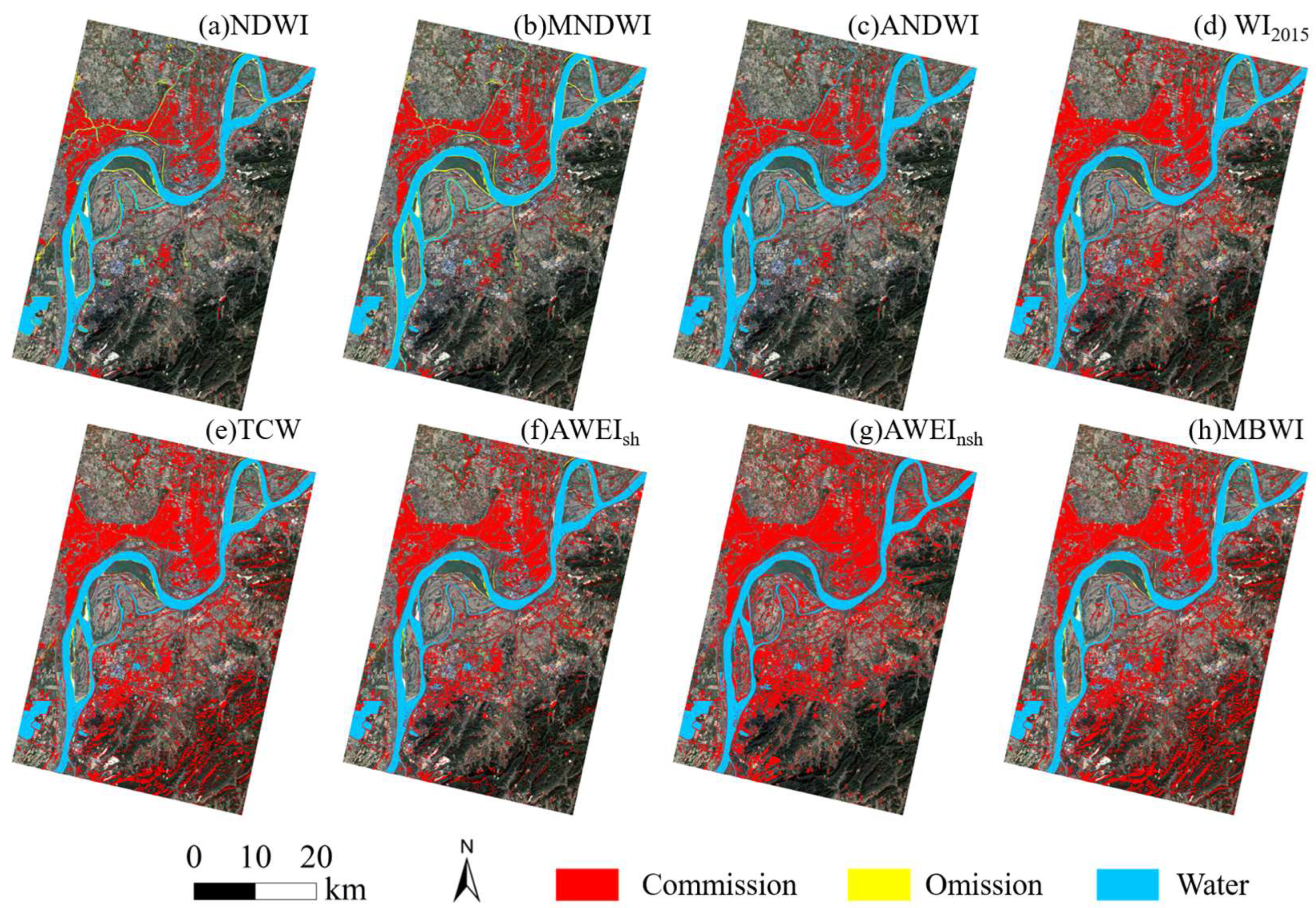
4.3. Comparison of Water Body Extraction

To evaluate the extraction performance of different water indices, three test sites featuring complex water body boundaries, large watersheds, and rivers of varying morphologies were selected. Overall, the eight water indices successfully captured the distribution of water bodies within each test site.

An analysis of the Lake Wivenhoe region using Landsat-9 imagery serves as a case study. Figure 8 illustrates that the primary areas of omission occur with the ratio-based indices NDWI, MNDWI, and ANDWI (Figure 8a–c), which tend to miss finer water bodies. In contrast, AWEI_nsh (Figure 8g) demonstrates the least amount of omission in capturing fine water bodies. The main misclassifications in the difference-based indices AWEI_nsh, MBWI, and TCW are related to mountain shadows and buildings. AWEI_nsh (Figure 8g) shows the highest misidentification of building shadows as water bodies, whereas WI₂₀₁₅ (Figure 8d) is less prone to this error. TCW (Figure 8e) tends to misclassify mountain shadows the most, whereas WI₂₀₁₅ (Figure 8d) effectively minimizes such errors.

The Mille Lacs Lake area shares similarities with the Lake Wivenhoe region in its inclusion of omissions in fine stream areas. In terms of ratio-based indices, NDWI, MNDWI, and ANDWI lack precision in identifying the boundaries of water bodies, resulting in more frequent omissions at the edges of smaller water areas (Figure 9a–c).

In the Tongling section of the Yangtze River region, disturbances from paddy fields and mountain shadows are prevalent, leading to high rates of misclassification across all eight water indices (Figure 10). TCW and MBWI (Figure 10e,h) show less effectiveness in suppressing mountain shadows and building shadows, often misidentifying these features as bodies of water. WI₂₀₁₅, AWEI_sh, and AWEI_nsh exhibit fewer errors with mountain shadows but tend to misclassify building shadows as water more frequently. In the other test sites, similar results were also observed (Figures S24–S27).

To compare the accuracy of different water indices using Landsat-8 and Landsat-9 imagery, an analysis was performed focusing on the extraction accuracies and Kappa and MCC statistics for each index. The results, summarized in

Table 4. Accuracy metrics of water mapping based on the Landsat-8 OLI and Landsat-9 OLI-2 data. (Note: red font represents the negative value).

Site		Landsat-9									Landsat-8 Minus Landsat-9
		NDWI	MNDWI	ANDWI	WI2015	TCW	AWEIsh	AWEInsh	MBWI		NDWI	MNDWI	ANDWI	WI2015	TCW	AWEIsh	AWEInsh	MBWI
Mille Lacs Lake	Kappa	0.574	0.364	0.437	0.822	0.843	0.820	0.780	0.838		−0.170	0.055	−0.089	0.015	−0.006	0.001	0.011	0.000
	OA	0.825	0.660	0.718	0.937	0.944	0.937	0.924	0.942		−0.132	0.048	−0.073	0.005	−0.002	0.000	0.005	0.000
	PA	0.834	0.561	0.645	0.980	0.986	0.986	0.986	0.980		−0.226	0.074	−0.108	0.003	−0.003	−0.003	0.011	0.000
	UA	0.925	0.976	0.970	0.939	0.942	0.933	0.918	0.945		0.048	−0.012	0.011	0.003	0.000	0.003	−0.002	0.000
	MCC	0.583	0.454	0.505	0.826	0.847	0.826	0.790	0.840		−0.101	0.034	−0.060	0.014	−0.007	−0.000	0.017	0.000
Lake Nipissing	Kappa	0.362	0.344	0.310	0.580	0.581	0.561	0.519	0.581		−0.129	0.071	0.041	−0.011	−0.020	0.000	−0.016	−0.016
	OA	0.675	0.658	0.639	0.791	0.791	0.782	0.763	0.791		−0.078	0.039	0.024	−0.006	−0.010	0.000	−0.007	−0.008
	PA	0.545	0.381	0.334	0.793	0.789	0.797	0.820	0.782		−0.279	0.069	0.066	−0.007	−0.024	−0.004	0.019	−0.006
	UA	0.784	0.957	0.981	0.813	0.816	0.797	0.758	0.820		0.156	0.011	−0.045	−0.004	−0.001	0.003	−0.017	−0.008
	MCC	0.382	0.439	0.421	0.581	0.581	0.561	0.521	0.582		−0.040	0.060	0.015	−0.011	−0.019	0.000	−0.013	−0.016
Tongling section of Yangtze River	Kappa	0.731	0.701	0.706	0.674	0.618	0.667	0.607	0.609		−0.030	−0.007	−0.023	0.002	−0.020	−0.014	−0.038	−0.014
	OA	0.867	0.851	0.854	0.836	0.806	0.832	0.801	0.801		−0.014	−0.003	−0.011	0.001	−0.010	−0.007	−0.019	−0.007
	PA	0.804	0.827	0.814	0.918	0.954	0.922	0.914	0.960		−0.070	−0.006	−0.031	−0.009	−0.015	−0.011	0.008	−0.019
	UA	0.903	0.852	0.867	0.775	0.723	0.768	0.731	0.715		0.038	−0.001	0.004	0.006	−0.006	−0.005	−0.026	−0.001
	MCC	0.735	0.701	0.707	0.685	0.647	0.679	0.624	0.642		−0.018	−0.006	−0.021	−0.000	−0.022	−0.015	−0.030	−0.019
Lianhuan Lake	Kappa	0.823	0.835	0.838	0.832	0.757	0.844	0.844	0.772		0.061	0.003	0.011	0.018	0.015	0.014	0.003	0.017
	OA	0.912	0.918	0.919	0.916	0.878	0.922	0.922	0.886		0.030	0.001	0.006	0.009	0.008	0.007	0.001	0.008
	PA	0.834	0.863	0.857	0.968	0.974	0.971	0.968	0.974		0.151	0.009	0.023	0.003	0.000	0.000	0.009	0.003
	UA	0.986	0.967	0.977	0.876	0.817	0.883	0.885	0.827		−0.080	−0.006	−0.012	0.012	0.010	0.012	−0.003	0.011
	MCC	0.833	0.840	0.844	0.837	0.771	0.848	0.847	0.784		0.055	0.002	0.009	0.016	0.013	0.013	0.004	0.016
Sai Lake	Kappa	0.668	0.681	0.674	0.715	0.726	0.670	0.580	0.735		−0.016	0.020	0.022	−0.012	−0.018	0.006	0.012	−0.034
	OA	0.831	0.838	0.834	0.859	0.864	0.838	0.797	0.868		−0.007	0.010	0.012	−0.006	−0.008	0.002	0.005	−0.016
	PA	0.743	0.744	0.736	0.844	0.841	0.848	0.872	0.834		0.004	0.020	0.030	−0.009	0.007	0.000	−0.008	0.004
	UA	0.951	0.963	0.965	0.903	0.914	0.865	0.793	0.927		−0.020	−0.001	−0.009	−0.004	−0.020	0.004	0.011	−0.032
	MCC	0.689	0.704	0.699	0.717	0.729	0.671	0.584	0.740		−0.020	0.016	0.015	−0.012	−0.019	0.005	0.010	−0.037
Liangzi Lake	Kappa	0.863	0.885	0.888	0.782	0.732	0.770	0.736	0.767		0.025	−0.041	−0.029	−0.019	0.022	−0.010	0.032	−0.013
	OA	0.933	0.943	0.945	0.890	0.864	0.884	0.866	0.882		0.012	−0.020	−0.015	−0.010	0.011	−0.005	0.017	−0.007
	PA	0.874	0.936	0.914	0.988	0.986	0.986	0.988	0.984		0.046	0.017	0.026	−0.009	0.000	−0.007	−0.017	−0.002
	UA	0.972	0.936	0.959	0.806	0.771	0.798	0.772	0.797		−0.018	−0.055	−0.053	−0.009	0.015	−0.003	0.033	−0.009
	MCC	0.866	0.885	0.889	0.798	0.755	0.787	0.759	0.784		0.022	−0.038	−0.029	−0.019	0.018	−0.011	0.022	−0.012
Lake Wivenhoe	Kappa	0.808	0.798	0.795	0.857	0.860	0.836	0.802	0.866		−0.043	−0.056	−0.053	−0.003	−0.006	−0.002	−0.026	−0.012
	OA	0.909	0.905	0.904	0.930	0.932	0.920	0.902	0.935		−0.019	−0.025	−0.024	−0.001	−0.003	−0.002	−0.013	−0.006
	PA	0.793	0.718	0.775	0.929	0.929	0.929	0.954	0.921		−0.050	−0.061	−0.057	−0.004	0.000	0.007	−0.015	0.000
	UA	0.987	0.99	0.991	0.906	0.909	0.884	0.834	0.921		0.003	−0.001	−0.001	0.000	−0.006	−0.008	−0.015	−0.013
	MCC	0.821	0.813	0.810	0.857	0.860	0.837	0.808	0.866		−0.036	−0.047	−0.044	−0.003	−0.006	−0.002	−0.027	−0.012

, demonstrate the consistency of extraction accuracies between Landsat-8 and Landsat-9, with the largest discrepancy observed in the PA of the NDWI index within Lake Nipissing, showing a difference of −0.279. In contrast, the smallest gaps (close to 0) in PA were detected in the Mille Lacs Lake (MBWI), Lake Wivenhoe (TCW and MBWI), Liangzi Lake (TCW), Sai Lake (AWEIsh), and Lianhuan Lake (TCW and AWEI_sh). Among all MCC results, the largest difference was observed in the NDWI of Mille Lacs Lake (−0.101); however, the smallest difference (close to 0) is the MBWI of Mille Lacs Lake, the AWEI_sh of Lake Nipissing and WI₂₀₁₅ of the Tongling section of the Yangtze River, indicating the perfect classifiers for water detection.

Among the indices, the NDWI index exhibited the greatest variability in accuracy differences, with several test sites showing a precision difference greater than 0.15 (in absolute value) between Landsat-8 and Landsat-9 data. For instance, the Kappa difference in the Mille Lacs Lake region reached −0.170, and the UA difference in Lake Nipissing was 0.156. The PA difference in Lianhuan Lake reached 0.151, and in Nipissing reached −0.279. The largest MCC difference of the NDWI reaches −0.101, and the smallest difference (−0.018) was observed in the Tongling section of the Yangtze River. The accuracy differences for all other indices across Landsat-8 and Landsat-9 data were below 0.1 (in absolute value), suggesting more attention should be given to the use of the NDWI index when applying Landsat-8 and Landsat-9 imagery concurrently.

The analysis shows that within the same test site, the PA for ratio-based indices was lower than that for difference-based indices. For example, in the Sai Lake region on Landsat-9 imagery, the PA for the three ratio-based indices (NDWI, MNDWI, and ANDWI) were 0.743, 0.744, and 0.736, respectively, while the PA for the other difference-based indices were all above 0.800. Similar patterns were observed in other sites on both datasets, where the PA for ratio-based indices was consistently lower than that for difference-based indices, and omissions were more frequent in ratio-based indices. In general, the results of OA and MCC are similar and complemental.

Furthermore, the UA for ratio-based indices was higher than that for difference-based indices within the test sites. For instance, in the Liangzi Lake region on Landsat-9 imagery, the UA for the three ratio-based indices (NDWI, MNDWI, and ANDWI) were 0.972, 0.936, and 0.959, respectively, whereas the UA for the other difference-based indices were all below 0.900. Accuracy results on both datasets in other sites showed the same trend (Table 4), where the UA for ratio-based indices was greater than the PA for difference-based indices, and the difference-based indices had a higher rate of misclassification compared to ratio-based indices.

5. Discussion

5.1. Performance and Effectiveness of Various Water Indices

The computation of remote sensing indices for water body detection is straightforward, eliminating the need for intricate training processes. This simplicity facilitates the rapid extraction of water body information over large areas, making it an essential technique for global and regional assessments of water distribution and area estimation. Despite a trend towards more complex water body indices, existing studies suggest that more elaborate indices do not always outperform their simpler counterparts [27]. In our research, we utilized eight different water indices for water extraction.

NDWI effectively minimizes the influence of non-aquatic elements like vegetation and soil, proving particularly effective for large lakes and reservoirs. However, it still includes substantial interference when applied to urban water bodies [29]. MNDWI, building upon the NDWI approach, uses the Landsat TM short-wave infrared band (TM5) instead of the near-infrared band (TM4). This modification enhances the index’s ability to reduce the impacts of soil and buildings, thereby improving the removal of shadows from urban structures [32]. AWEI, including its variants AWEI_nsh and AWEI_sh, is formulated based on TM image data. AWEI aims to maximally separate aquatic from non-aquatic pixels through band subtraction and the application of varying coefficients. Validation has shown that AWEI achieves higher accuracy in water extraction than MNDWI [28]. Building on WI₂₀₀₆, the WI₂₀₁₅ introduces a new extraction algorithm based on linear discriminant analysis (LDA), employing the LDA classification (LDAC) to determine optimal coefficients for segregating training area classes, thereby enhancing classification precision [35]. The MBWI mitigates the effects of mountain shadows and dark building pixels while also lessening seasonal variations caused by changes in solar conditions [33]. The TCT, an empirical orthogonal transformation introduced by Kauth et al. [53] during studies on crop growth stages, effectively extracts water information through its wetness component (i.e., TCW), as utilized in our research.

Figure 11 displays the precision statistics across eight water indices at various test sites. Under differing surface water environmental conditions, the OA fluctuations of the NDWI, MNDWI, and ANDWI indices are notably larger compared to the other indices, highlighting the superior robustness of AWEI_nsh, AWEI_sh, WI₂₀₁₅, TCW, and MBWI in water body extraction, which can be mutually confirmed with MCC results. Generally, the results of OA and MCC are similar. Analyzing PA results, the ratio-based indices (NDWI, MNDWI, and ANDWI) exhibit greater variability and generally lower mean values compared to the difference-based indices, resulting in a higher incidence of omission errors, as depicted in Figure 8, Figure 9 and Figure 10. Conversely, UA analysis shows that ratio-based indices have higher mean values, indicating fewer commission errors, while difference-based indices exhibit lower mean values and, thus, more commission errors.

As shown in Figure 11 and Figure 12 across various study areas, the NDWI index performs less effectively in water body extraction compared to AWEI_sh. AWEIs_h demonstrates superior capability in identifying small water bodies within images, outperforming NDWI, which tends to misclassify water body edges as non-water, leading to increased omission errors and impacting overall accuracy. According to our findings, the water extraction accuracy based on Landsat-8 and Landsat-9 imagery is consistent. The related results suggest that the subtle differences between the two sensors do not lead to significant variations in accuracy. Consequently, we can confidently utilize data from both sensors in tandem for water body mapping across various temporal and spatial scales.

Through systematic analysis and comparison of various water body indices applied to Landsat-8 and Landsat-9 imagery, the results demonstrated the distinct advantages and limitations inherent to both ratio-based and difference-based indices. Our results confirm that ratio-based indices like NDWI, MNDWI, and ANDWI exhibit significant variability in accuracy, especially in complex urban and boundary water body scenarios. They offer stable performance across diverse environments and satellites due to their ability to mitigate the effects of clouds and shadows without the need for coefficients. On the other hand, difference-based indices such as AWEI_sh, WI₂₀₁₅, TCW, and MBWI, despite their empirical coefficients and potential for variability, have shown higher robustness in extracting water bodies, particularly in challenging conditions where the precision and minimization of omission and commission errors are critical.

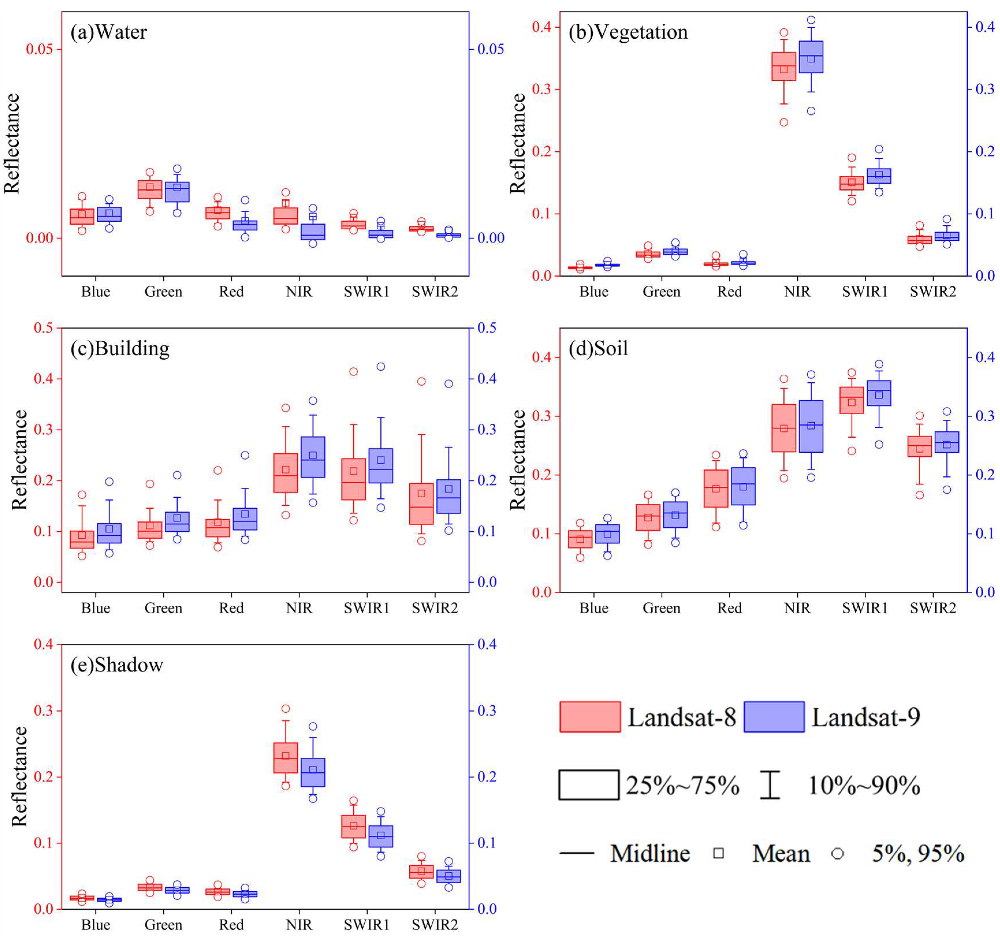
5.2. Spectral Response and Reflectance of Landsat-8 and Landsat-9 Data

Landsat-9 is the latest addition to the Landsat satellite series, continuing the mission of Earth observation established by its predecessors. Moreover, one of its significant roles is to work in tandem with Landsat-8 to halve the Earth observation cycle from 16 d to 8 d [21,39]. This necessitates a high degree of consistency in the imagery data between Landsat-9 and Landsat-8 to ensure the results from both are strictly comparable [54]. The primary distinctions between them stem from differences in spectral reflectance attributed to their spectral response functions [21].

Regarding the remote sensors, there are some disparities in the spectral band ranges of the Landsat-8 OLI and Landsat-9 OLI-2 (

Table 5. The basic specifications for the spectral characteristics and spatial resolution of OLI and OLI-2 sensors.

Band	Acronym	Spatial Resolution	Landsat-8 OLI		Landsat-9 OLI2
			Spectral Range	Band Center	Spectral Range	Band Center
Coastal aerosol	B1	30 m	433–453	443	435–451	443
Blue (B)	B2	30 m	450–515	483	452–512	482
Green (G)	B3	30 m	525–600	561	533–590	562
Red (R)	B4	30 m	630–680	655	636–673	655
Near-infrared (NIR)	B5	30 m	845–885	865	851–879	866
Shortwave infrared 1 (SWIR1)	B6	30 m	1560–1660	1610	1566–1651	1610
Shortwave infrared 2 (SWIR2)	B7	30 m	2100–2300	2200	2107–2294	2201
Panchromatic	B8	15 m	500–680	591	503–676	590
Cirrus	B9	30 m	1360–1390	1373	1363–1384	1374

). For instance, the bands used to calculate NDWI, the Green and NIR bands, have wavelengths of 525–600 nm and 845–885 nm for Landsat 8 OLI, compared to 533–590 nm and 851–879 nm for Landsat 9 OLI-2, respectively. Additionally, there are differences in reflectance in the SWIR bands. This is because they share similar spectral response functions with some differences (Figure 12). The spectral response peaks for SWIR2, SWIR1, NIR, Green, and Red bands on Landsat-9 OLI-2 are higher than those on Landsat-8 OLI, suggesting that OLI-2 is more sensitive to these wavelengths.

Another critical metric for assessing the performance of remote sensing instruments is the signal-to-noise ratio (SNR) [54]. Under typical radiation conditions, the SNR of data transmitted by OLI-2 on Landsat-9 is improved by 25%, offering higher radiometric precision in observing the Earth’s surface. Landsat-9’s OLI-2 downlink transmits all 14-bit data produced by the spacecraft’s electronic equipment to Earth, providing images with greater bit depth and redundancy [41,55].

Reflectance serves as the data foundation for distinguishing different land cover types. The varying chemical compositions, physical structures, and surface states influence the capacities for reflecting, absorbing, and transmitting electromagnetic waves. In this study, we selected “pure” pixel samples from the same locations in both Landsat-8 and Landsat-9 imagery to provide a reference for the spectral differences between the two sets of images. These “pure” pixels with a size of 30 × 30 m were obtained from seven test sites covered by Landsat-8 and Landsat-9 imagery. Figure 13 displayed the typical “pure” pixels in the Landsat scene. They encompass all the challenging factors of identifying surface water: mountain shadows, urban areas (buildings), vegetation, and bare soil.

Utilizing remote sensing imagery, high-resolution Google Earth images, and the Chinese MapWorld database, a total of 1768 pure pixel samples were selected. Regardless of the land cover type, certain discrepancies exist in the reflectance of pure land cover pixels across the six spectral bands between Landsat-8 and Landsat-9 data (Figure 14). Notably, the reflectance of the NIR band exhibits a significant difference between Landsat-8 OLI and Landsat-9 OLI-2, impacting the construction of various water indices. Except for the MNDWI index, which does not utilize the NIR band, all others in this study incorporated this specific band in their formulation. The comparative analysis revealed a smaller discrepancy in water body extraction accuracy between Landsat-8 and Landsat-9 for the MNDWI index compared to others, likely due to the exclusion of the NIR band.

5.3. Uncertainty and Perspective

Some existed studies analyzed the differences between Landsat-8 and Landsat-9 satellite data, and the results suggest that Landsat 9 closely resembles Landsat 8 in various aspects and has similar reflected wavelengths and find suitability for both satellite datasets for water detection [21,56]. The significant differences in the average absolute percentage change in the bands may affect the water detections. However, whether the deviation in the calculation of water indices affects the mapping performances is still unclear. Therefore, we conducted a comparative analysis of the performance in water body extraction between Landsat-8 and Landsat-9 satellite data in this study. Our research, leveraging eight distinct water indices, aimed to extract water bodies at seven sites globally from Landsat-8 and Landsat-9. That is the main academic contribution and novelty of this study. The findings indicate a good consistency between the Landsat-9 and Landsat-8 satellites, with the former demonstrating superior performance.

The selection of image data is pivotal to ensuring the accuracy of cross-comparisons, necessitating the use of synchronized image pairs. The most reliable data are the cross under-fly data provided by the United States Geological Survey (USGS), where Landsat 9 and Landsat 8 pass overhead almost simultaneously, with temporal discrepancies as minimal as a few seconds and no more than three minutes and nearly identical solar azimuth and elevation angles [55]. This minimizes the potential discrepancies arising from atmospheric and illumination conditions. The results in [39,54] have leveraged these data to analyze the differences between the two sensors, illustrating this approach.

It is crucial to note, however, that the Landsat-8 and Landsat-9 data used in this study were still separated by 1d. Water bodies can undergo changes within a single day, particularly in arid regions [13], which may influence the outcomes of this study. Moreover, the selection of water bodies was somewhat limited, primarily due to the multiple considerations of acquisition date (minimum temporal gap), image quality (cloud cover), geographical distribution, and water body coverage in our selection of remote sensing imagery. For the accuracy assessment, this study mainly relied on visual interpretation results of employed Landsat-8 and Landsat-9 imagery. The high-resolution Google Earth imagery and Chinese MapWorld database were also utilized to distinguish between water and non-water classes, especially for indistinguishable pixels on 30 m Landsat scenes. However, these datasets might have been compiled and integrated from remote sensing images acquired over adjacent periods (within several weeks before or after the primary acquisition dates). Although the temporal differences between the Landsat and high-resolution reference datasets may introduce potential uncertainties, in this study, the imagery was captured over the same scene and within a 24 h interval, minimizing any impact on the final results. In future studies, we aim to increase the number of reference data by incorporating additional field sites to reduce uncertainty and enable more robust comparisons.

In this study, we utilized level 2 science products (L2SP) available on the Google Earth Engine (GEE) platform, employing the atmospheric correction algorithm from the Land Surface Reflectance Code (LaSRC) algorithm (Version 3.5.5) [57]. Although Landsat-8 and Landsat-9 are sibling satellites, certain improvements or modifications to the OLI-2 sensor on Landsat-9 compared to the OLI sensor could account for some of the observed discrepancies in water body extraction results caused by identical surface reflectance computations. In addition, the different performance of various indices between Landsat-8 and Landsat-9 data can be attributed to variability of reflectance spectra caused by concentrations of phytoplankton and sediments, depth, and/or substratum type [58]. For example, Lianhuan Lake is a typical shallow water area (average depth < 0.5 m), and regional aquatic plants are flourishing. Liangzi Lake is characterized by dense phytoplankton. These facts might result in possible spectral variations (as well as water index values) affecting the water mapping accuracy.

Threshold segmentation is a commonly employed method for water body extraction, yet the setting of the threshold significantly influences the separation outcome [8]. An excessively high threshold may lead to omission errors, particularly for smaller water bodies, while a low threshold can introduce considerable noise [46]. The subjectivity inherent in manually setting thresholds is undeniable. Beyond logical operations, water index thresholds predominantly utilize empirical (global) thresholds and bisection (local adaptive) thresholds, with the key to threshold applicability lying in its ability to differentiate the subtle distinctions between mixed water and non-water pixels [59]. In fact, the optimal threshold is only available in ideal conditions since it is dependent not only on the sensor but also on the scene. To mitigate the subjectivity of empirical thresholds, this study employed the Otsu method for determining the segmentation threshold. Algorithms like the Otsu method and histogram bimodality are standard for threshold segmentation but are not without limitations, especially in complex environments. Li et al. [56] explored the usability of Landsat-9 images in the relationship between the extraction accuracy and the algorithm; the results indicated that the fixed threshold may cause the significantly distorted overall accuracy of water mapping. Studies have shown that the Otsu method’s optimal threshold for the NDWI index is 0.18 [59], significantly lower than the actual optimal value (0.38) obtained by the minimum thresholding method. Further research demonstrated that the accuracy gap between the Otsu threshold and manually determined optimal thresholds could reach up to 9–200% [60,61], suggesting the Otsu threshold may not be suitable for all case areas or for indices with unimodal distributions. In addition, this specific method is sensitive to the proportion of water vs. non-water pixels. In this study, we found that the impact of the polygon size on Otsu threshold and subsequently on water extraction accuracy is limited. This can be attributed to the distinctive class separability between water and non-water classes. Nevertheless, it is noted that the performance of Otsu method for threshold segmentation in this study is satisfactory. In addition, though not implemented in our current study, we intend to do so in the future so the modified Otsu method can identify the robust threshold of various water indices and believe we can further reduce the uncertainty and improve the accuracy of the water mapping.

The pivotal role of the Landsat series in water body remote sensing research is undeniable. With the confirmation that the Landsat-9 satellite can accurately map surface water, the future holds promise for achieving high-spatiotemporal resolution Earth observations at more detailed temporal intervals [21]. By integrating emerging technologies such as deep learning, we can precisely depict land cover changes and their impacts on surface water resources, crafting comprehensive solutions for assessing progress towards SDG-6 indicators.

6. Conclusions

The Landsat program has functioned much like a relay runner, launching a series of satellites that have conducted Earth observations for over 50 years. This enduring initiative has continually passed the baton from one satellite to the next, ensuring a consistent and valuable flow of data to monitor and study our planet’s environment and changes. In this study, we analyze the performance of almost simultaneous Landsat-8 and Landsat-9 data for water body extraction based on eight common water indices (NDWI, MNDWI, ANDWI, WI₂₀₁₅, TCW, AWEI_sh, AWEI_nsh, and MBWI) to extract water bodies in seven study sites worldwide. The Otsu algorithm is utilized to automatically determine the optimal segmentation threshold for water body extraction. From the perspective of the extraction performance of each index, we investigated the effect of both satellite data. The results showed the following:

(1)

Landsat-9 satellite data can be used for water body extraction effectively, with results consistent with those from Landsat-8. The selected eight water indices in this study are applicable on both Landsat-8 and Landsat-9 satellites.

(2)

The NDWI index shows a larger variability in accuracy compared to other indices when used on Landsat-8 and Landsat-9 imagery. Therefore, additional caution should be exercised when using the NDWI for water body analysis with both Landsat-8 and Landsat-9 satellites simultaneously.

(3)

For Landsat-8 and Landsat-9 imagery, ratio-based water indices tend to have more omission errors, while difference-based indices are more prone to commission errors. All water indices can enhance water information and suppress background noise. Among them, TCW and MBWI show less effective suppression of mountain shadows, while AWEI_nsh performs well in extracting fine rivers but poorly in suppressing building information, leading to more misclassification. Overall, ratio-based indices exhibit greater variability in overall accuracy, whereas difference-based indices demonstrate lower sensitivity to variations in the study area, showing smaller overall accuracy fluctuations and higher robustness.

Last but not least, the combined use of Landsat-8 and Landsat-9 is promising, particularly for water extraction. However, different water index methods exhibit unique characteristics under various environmental conditions, and the most suitable method should be selected based on specific circumstances.

References

1. Pekel, J.-F.; Cottam, A.; Gorelick, N.; Belward, A.S. High-resolution mapping of global surface water and its long-term changes. Nature 2016, 540, 418–422. [Google Scholar] [CrossRef] [PubMed]
2. Huang, C.; Chen, Y.; Zhang, S.; Wu, J. Detecting, Extracting, and Monitoring Surface Water From Space Using Optical Sensors: A Review. Rev. Geophys. 2018, 56, 333–360. [Google Scholar] [CrossRef]
3. Jordan, Y.C.; Ghulam, A.; Hartling, S. Traits of surface water pollution under climate and land use changes: A remote sensing and hydrological modeling approach. Earth-Sci. Rev. 2014, 128, 181–195. [Google Scholar] [CrossRef]
4. Chang, N.-B.; Imen, S.; Vannah, B. Remote Sensing for Monitoring Surface Water Quality Status and Ecosystem State in Relation to the Nutrient Cycle: A 40-Year Perspective. Crit. Rev. Environ. Sci. Technol. 2015, 45, 101–166. [Google Scholar] [CrossRef]
5. Sogno, P.; Klein, I.; Kuenzer, C. Remote Sensing of Surface Water Dynamics in the Context of Global Change—A Review. Remote Sens. 2022, 14, 2475. [Google Scholar] [CrossRef]
6. Tran, T.N.D.; Do, S.K.; Nguyen, B.Q.; Tran, V.N.; Grodzka-Łukaszewska, M.; Sinicyn, G.; Lakshmi, V. Investigating the Future Flood and Drought Shifts in the Transboundary Srepok River Basin Using CMIP6 Projections. IEEE J. Sel. Top. Appl. Earth Obs. Remote Sens. 2024, 17, 7516–7529. [Google Scholar] [CrossRef]
7. Ge, X.; Ding, J.; Amantai, N.; Xiong, J.; Wang, J. Responses of vegetation cover to hydro-climatic variations in Bosten Lake Watershed, NW China. Front. Plant Sci. 2024, 15, 1323445. [Google Scholar] [CrossRef] [PubMed]
8. Yang, X.; Qin, Q.; Yésou, H.; Ledauphin, T.; Koehl, M.; Grussenmeyer, P.; Zhu, Z. Monthly estimation of the surface water extent in France at a 10-m resolution using Sentinel-2 data. Remote Sens. Environ. 2020, 244, 111803. [Google Scholar] [CrossRef]
9. Pickens, A.H.; Hansen, M.C.; Hancher, M.; Stehman, S.V.; Tyukavina, A.; Potapov, P.; Marroquin, B.; Sherani, Z. Mapping and sampling to characterize global inland water dynamics from 1999 to 2018 with full Landsat time-series. Remote Sens. Environ. 2020, 243, 111792. [Google Scholar] [CrossRef]
10. Luo, X.; Tong, X.; Hu, Z. An applicable and automatic method for earth surface water mapping based on multispectral images. Int. J. Appl. Earth Obs. Geoinf. 2021, 103, 102472. [Google Scholar] [CrossRef]
11. Palmer, S.C.; Kutser, T.; Hunter, P.D. Remote sensing of inland waters: Challenges, progress and future directions. Remote Sens. Environ. 2015, 157, 1–8. [Google Scholar] [CrossRef]
12. Yang, X.; Chen, L. Evaluation of automated urban surface water extraction from Sentinel-2A imagery using different water indices. J. Appl. Remote Sens. 2017, 11, 026016. [Google Scholar] [CrossRef]
13. Wang, J.; Ding, J.; Li, G.; Liang, J.; Yu, D.; Aishan, T.; Zhang, F.; Yang, J.; Abulimiti, A.; Liu, J. Dynamic detection of water surface area of Ebinur Lake using multi-source satellite data (Landsat and Sentinel-1A) and its responses to changing environment. CATENA 2019, 177, 189–201. [Google Scholar] [CrossRef]
14. Yang, X.; Zhao, S.; Qin, X.; Zhao, N.; Liang, L. Mapping of Urban Surface Water Bodies from Sentinel-2 MSI Imagery at 10 m Resolution via NDWI-Based Image Sharpening. Remote Sens. 2017, 9, 596. [Google Scholar] [CrossRef]
15. Duan, Y.; Zhang, W.; Huang, P.; He, G.; Guo, H. A New Lightweight Convolutional Neural Network for Multi-Scale Land Surface Water Extraction from GaoFen-1D Satellite Images. Remote Sens. 2021, 13, 4576. [Google Scholar] [CrossRef]
16. Petrakis, R.E.; Soulard, C.E.; Waller, E.K.; Walker, J.J. Analysis of Surface Water Trends for the Conterminous United States Using MODIS Satellite Data, 2003–2019. Water Resour. Res. 2022, 58, e2021WR031399. [Google Scholar] [CrossRef]
17. Li, L.; Skidmore, A.; Vrieling, A.; Wang, T. A new dense 18-year time series of surface water fraction estimates from MODIS for the Mediterranean region. Hydrol. Earth Syst. Sci. 2019, 23, 3037–3056. [Google Scholar] [CrossRef]
18. Ogilvie, A.; Belaud, G.; Massuel, S.; Mulligan, M.; Le Goulven, P.; Calvez, R. Surface water monitoring in small water bodies: Potential and limits of multi-sensor Landsat time series. Hydrol. Earth Syst. Sci. 2018, 22, 4349–4380. [Google Scholar] [CrossRef]
19. Alsdorf, D.E.; Rodríguez, E.; Lettenmaier, D.P. Measuring surface water from space. Rev. Geophys. 2007, 45, RG2002. [Google Scholar] [CrossRef]
20. Hemati, M.; Hasanlou, M.; Mahdianpari, M.; Mohammadimanesh, F. A Systematic Review of Landsat Data for Change Detection Applications: 50 Years of Monitoring the Earth. Remote Sens. 2021, 13, 2869. [Google Scholar] [CrossRef]
21. Masek, J.G.; Wulder, M.A.; Markham, B.; McCorkel, J.; Crawford, C.J.; Storey, J.; Jenstrom, D.T. Landsat 9: Empowering open science and applications through continuity. Remote Sens. Environ. 2020, 248, 111968. [Google Scholar] [CrossRef]
22. Showstack, R. Landsat 9 Satellite Continues Half-Century of Earth Observations: Eyes in the sky serve as a valuable tool for stewardship. BioScience 2022, 72, 226–232. [Google Scholar] [CrossRef]
23. Chen, J.; Chen, S.; Fu, R.; Li, D.; Jiang, H.; Wang, C.; Peng, Y.; Jia, K.; Hicks, B.J. Remote Sensing Big Data for Water Environment Monitoring: Current Status, Challenges, and Future Prospects. Earth’s Future 2022, 10, e2021EF002289. [Google Scholar] [CrossRef]
24. Bijeesh, T.V.; Narasimhamurthy, K.N. Surface water detection and delineation using remote sensing images: A review of methods and algorithms. Sustain. Water Resour. Manag. 2020, 6, 68. [Google Scholar] [CrossRef]
25. Liu, S.; Wu, Y.; Zhang, G.; Lin, N.; Liu, Z. Comparing Water Indices for Landsat Data for Automated Surface Water Body Extraction under Complex Ground Background: A Case Study in Jilin Province. Remote Sens. 2023, 15, 1678. [Google Scholar] [CrossRef]
26. Kaplan, G.; Avdan, U. Object-based water body extraction model using Sentinel-2 satellite imagery. Eur. J. Remote Sens. 2017, 50, 137–143. [Google Scholar] [CrossRef]
27. Zhou, Y.; Dong, J.; Xiao, X.; Xiao, T.; Yang, Z.; Zhao, G.; Zou, Z.; Qin, Y. Open surface water mapping algorithms: A comparison of water-related spectral indices and sensors. Water 2017, 9, 256. [Google Scholar] [CrossRef]
28. Feyisa, G.L.; Meilby, H.; Fensholt, R.; Proud, S.R. Automated Water Extraction Index: A new technique for surface water mapping using Landsat imagery. Remote Sens. Environ. 2014, 140, 23–35. [Google Scholar] [CrossRef]
29. Zhang, F.; Tiyip, T.; Kung, H.-t.; Johnson, V.C.; Wang, J.; Nurmemet, I. Improved water extraction using Landsat TM/ETM+ images in Ebinur Lake, Xinjiang, China. Remote Sens. Appl. Soc. Environ. 2016, 4, 109–118. [Google Scholar] [CrossRef]
30. Ma, S.; Zhou, Y.; Gowda, P.H.; Dong, J.; Zhang, G.; Kakani, V.G.; Wagle, P.; Chen, L.; Flynn, K.C.; Jiang, W. Application of the water-related spectral reflectance indices: A review. Ecol. Indic. 2019, 98, 68–79. [Google Scholar] [CrossRef]
31. McFeeters, S.K. The use of the Normalized Difference Water Index (NDWI) in the delineation of open water features. Int. J. Remote Sens. 1996, 17, 1425–1432. [Google Scholar] [CrossRef]
32. Xu, H. Modification of normalised difference water index (NDWI) to enhance open water features in remotely sensed imagery. Int. J. Remote Sens. 2006, 27, 3025–3033. [Google Scholar] [CrossRef]
33. Wang, X.; Xie, S.; Zhang, X.; Chen, C.; Guo, H.; Du, J.; Duan, Z. A robust Multi-Band Water Index (MBWI) for automated extraction of surface water from Landsat 8 OLI imagery. Int. J. Appl. Earth Obs. Geoinf. 2018, 68, 73–91. [Google Scholar] [CrossRef]
34. Fisher, A.; Flood, N.; Danaher, T. Comparing Landsat water index methods for automated water classification in eastern Australia. Remote Sens. Environ. 2016, 175, 167–182. [Google Scholar] [CrossRef]
35. Rad, A.M.; Kreitler, J.; Sadegh, M. Augmented Normalized Difference Water Index for improved surface water monitoring. Environ. Model. Softw. 2021, 140, 105030. [Google Scholar] [CrossRef]
36. Baig, M.H.A.; Zhang, L.; Shuai, T.; Tong, Q. Derivation of a tasselled cap transformation based on Landsat 8 at-satellite reflectance. Remote Sens. Lett. 2014, 5, 423–431. [Google Scholar] [CrossRef]
37. Du, Z.; Li, W.; Zhou, D.; Tian, L.; Ling, F.; Wang, H.; Gui, Y.; Sun, B. Analysis of Landsat-8 OLI imagery for land surface water mapping. Remote Sens. Lett. 2014, 5, 672–681. [Google Scholar] [CrossRef]
38. Liu, Z.; Yao, Z.; Wang, R. Assessing methods of identifying open water bodies using Landsat 8 OLI imagery. Environ. Earth Sci. 2016, 75, 873. [Google Scholar] [CrossRef]
39. Xu, H.; Ren, M.; Lin, M. Cross-comparison of Landsat-8 and Landsat-9 data: A three-level approach based on underfly images. GIScience Remote Sens. 2024, 61, 2318071. [Google Scholar] [CrossRef]
40. Markham, B.; Jenstrom, D.; Masek, J.; Dabney, P.; Pedelty, J.; Barsi, J.; Montanaro, M. Landsat 9: Status and Plans; SPIE: Bellingham, WA, USA, 2016; Volume 9972. [Google Scholar] [CrossRef]
41. Niroumand-Jadidi, M.; Bovolo, F.; Bresciani, M.; Gege, P.; Giardino, C. Water Quality Retrieval from Landsat-9 (OLI-2) Imagery and Comparison to Sentinel-2. Remote Sens. 2022, 14, 4596. [Google Scholar] [CrossRef]
42. Albertini, C.; Gioia, A.; Iacobellis, V.; Manfreda, S. Detection of surface water and floods with multispectral satellites. Remote Sens. 2022, 14, 6005. [Google Scholar] [CrossRef]
43. Zhao, B.; Wu, J.; Han, X.; Tian, F.; Liu, M.; Chen, M.; Lin, J. An improved surface water extraction method by integrating multi-type priori information from remote sensing. Int. J. Appl. Earth Obs. Geoinf. 2023, 124, 103529. [Google Scholar]
44. Ostu, N. A threshold selection method from gray-level histograms. IEEE Trans. Syst. Man Cybern. 1979, 9, 62–69. [Google Scholar]
45. Rosser, J.F.; Leibovici, D.G.; Jackson, M.J. Rapid flood inundation mapping using social media, remote sensing and topographic data. Nat. Hazards 2017, 87, 103–120. [Google Scholar] [CrossRef]
46. Yang, X.; Chen, Y.; Wang, J. Combined use of Sentinel-2 and Landsat 8 to monitor water surface area dynamics using Google Earth Engine. Remote Sens. Lett. 2020, 11, 687–696. [Google Scholar] [CrossRef]
47. Günen, M.A.; Atasever, U.H. Remote sensing and monitoring of water resources: A comparative study of different indices and thresholding methods. Sci. Total Environ. 2024, 926, 172117. [Google Scholar] [CrossRef] [PubMed]
48. Pan, F.; Xi, X.; Wang, C. A Comparative Study of Water Indices and Image Classification Algorithms for Mapping Inland Surface Water Bodies Using Landsat Imagery. Remote Sens. 2020, 12, 1611. [Google Scholar] [CrossRef]
49. Haas, E.M.; Bartholomé, E.; Lambin, E.F.; Vanacker, V. Remotely sensed surface water extent as an indicator of short-term changes in ecohydrological processes in sub-Saharan Western Africa. Remote Sens. Environ. 2011, 115, 3436–3445. [Google Scholar] [CrossRef]
50. Matthews, B.W. Comparison of the predicted and observed secondary structure of T4 phage lysozyme. Biochim. Et Biophys. Acta (BBA)-Protein Struct. 1975, 405, 442–451. [Google Scholar] [CrossRef]
51. Prakash, N.; Manconi, A.; Loew, S. Mapping Landslides on EO Data: Performance of Deep Learning Models vs. Traditional Machine Learning Models. Remote Sens. 2020, 12, 346. [Google Scholar] [CrossRef]
52. Chen, F.; Chen, X.; Van de Voorde, T.; Roberts, D.; Jiang, H.; Xu, W. Open water detection in urban environments using high spatial resolution remote sensing imagery. Remote Sens. Environ. 2020, 242, 111706. [Google Scholar] [CrossRef]
53. Kauth, R.J.; Thomas, G. The Tasselled Cap—A Graphic Description of the Spectral-Temporal Development of Agricultural Crops as Seen by Landsat; Purdue University: West Lafayette, IN, USA, 1976; p. 159. [Google Scholar]
54. Xu, H.; Ren, M.; Yang, L. Evaluating the consistency of surface brightness, greenness, and wetness observations between Landsat-8 OLI and Landsat-9 OLI2 through underfly images. Int. J. Appl. Earth Obs. Geoinf. 2023, 124, 103546. [Google Scholar] [CrossRef]
55. Gross, G.; Helder, D.; Begeman, C.; Leigh, L.; Kaewmanee, M.; Shah, R. Initial Cross-Calibration of Landsat 8 and Landsat 9 Using the Simultaneous Underfly Event. Remote Sens. 2022, 14, 2418. [Google Scholar] [CrossRef]
56. Li, X.; Zhang, D.; Jiang, C.; Zhao, Y.; Li, H.; Lu, D.; Qin, K.; Chen, D.; Liu, Y.; Sun, Y. Comparison of lake area extraction algorithms in Qinghai Tibet plateau leveraging google earth engine and landsat-9 data. Remote Sens. 2022, 14, 4612. [Google Scholar] [CrossRef]
57. Vermote, E.; Justice, C.; Claverie, M.; Franch, B. Preliminary analysis of the performance of the Landsat 8/OLI land surface reflectance product. Remote Sens. Environ. 2016, 185, 46–56. [Google Scholar] [CrossRef] [PubMed]
58. Wang, J.; Shi, T.; Yu, D.; Teng, D.; Ge, X.; Zhang, Z.; Yang, X.; Wang, H.; Wu, G. Ensemble machine-learning-based framework for estimating total nitrogen concentration in water using drone-borne hyperspectral imagery of emergent plants: A case study in an arid oasis, NW China. Environ. Pollut. 2020, 266, 115412. [Google Scholar] [CrossRef] [PubMed]
59. Sekertekin, A. A Survey on Global Thresholding Methods for Mapping Open Water Body Using Sentinel-2 Satellite Imagery and Normalized Difference Water Index. Arch. Comput. Methods Eng. 2021, 28, 1335–1347. [Google Scholar] [CrossRef]
60. Mukherjee, A.; Kumar, A.A.; Ramachandran, P. Development of new index-based methodology for extraction of built-up area from landsat7 imagery: Comparison of performance with svm, ann, and existing indices. IEEE Trans. Geosci. Remote Sens. 2020, 59, 1592–1603. [Google Scholar] [CrossRef]
61. Li, C.; Shao, Z.; Zhang, L.; Huang, X.; Zhang, M. A comparative analysis of index-based methods for impervious surface mapping using multiseasonal Sentinel-2 satellite data. IEEE J. Sel. Top. Appl. Earth Obs. Remote Sens. 2021, 14, 3682–3694. [Google Scholar] [CrossRef]
Figure 1. Overview of all selected test sites. (a) Locations of the seven test sites, (b) Mille Lacs Lake, (c) Lake Nipissing region, (d) Tongling section of Yangtze River, (e) Lianhuan Lake, (f) Sai Lake, (g) Liangzi Lake, and (h) Lake Wivenhoe. All satellite maps are produced via Landsat-9 data (standard true color composite).
Remotesensing 16 01984 g001
Figure 2. Satellite map (standard true color composite) and various water indices map based on Landsat-9 in Tongling section of Yangtze River region.
Remotesensing 16 01984 g002
Figure 3. Differences of water indices maps between Landsat-8 and Landsat-9 data in Lake Wivenhoe region.
Remotesensing 16 01984 g003
Figure 4. Differences of water index maps between Landsat-8 and Landsat-9 data in Mille Lacs Lake region.
Remotesensing 16 01984 g004
Figure 5. Correlation analysis of water indices in the Lake Wivenhoe region based on Landsat-8 and Landsat-9 imagery (Note: red line denotes the fitted line).
Remotesensing 16 01984 g005
Figure 6. Comparison of the separability of different water indices based on Landsat-8 and Landsat-9 imagery in Lake Wivenhoe.
Remotesensing 16 01984 g006
Figure 7. Comparison of the applicability of different water body index thresholds based on Landsat-8 and Landsat-9 imagery in Lake Wivenhoe. (a) NDWI, (b) MNDWI, (c) ANDWI, (d) WI2015, (e) TCW, (f) AWEIsh, (g) AWEInsh, and (h) MBWI.
Remotesensing 16 01984 g007
Figure 8. Spatial differences in water index extraction capacity in the Lake Wivenhoe region based on Landsat-9 imagery.
Remotesensing 16 01984 g008
Figure 9. Spatial differences in water index extraction capacity in the Mille Lacs Lake region based on Landsat-9 imagery.
Remotesensing 16 01984 g009
Figure 10. Spatial differences in water index extraction capacity in the Tongling section of the Yangtze River region based on Landsat-9 imagery.
Remotesensing 16 01984 g010
Figure 11. Statistical results of statistical parameters across eight water indices. (a) Kappa, (b) OA, (c) PA, (d) UA, and (e) MCC.
Remotesensing 16 01984 g011
Figure 12. Comparison of spectral response curves between Landsat-8 OLI and Landsat-9 OLI-2. Spectral response functions obtained from https://landsat.gsfc.nasa.gov/satellites/landsat-8/spacecraft-instruments/ (last accessed on 12 May 2024) and https://landsat.gsfc.nasa.gov/satellites/landsat-9/landsat-9-instruments (last accessed on 12 May 2024), respectively.
Remotesensing 16 01984 g012
Figure 13. Spatial distribution of “pure” pixels in Landsat scene (standard true color composite) in Tongling section of Yangtze River. The number in (a) is the image id, and the number in (b) is the scene that corresponds to each image, where id (1–7) represent water, id (8–9) represent building, id (10–11) represent vegetation, id (12–13) represent bare soil, and id (14–15) represent mountain shadows.
Remotesensing 16 01984 g013
Figure 14. Surface reflectance of various land cover pixels in Landsat-8 and Landsat-9 imagery.
Remotesensing 16 01984 g014