Abstract
Accurate estimation of livestock carrying capacity (LCC) and implementation of an appropriate actual stocking rate (ASR) are key to the sustainable management of grazing adapted alpine grassland ecosystems. The reliable determination of aboveground biomass is fundamental to these determinations. Peak aboveground biomass (AGBP) captured from satellite data at the peak of the growing season (POS) is widely used as a proxy for annual aboveground biomass (AGBA) to estimate LCC of grasslands. Here, we demonstrate the limitations of this approach and highlight the ability of POS in the estimation of ASR. We develop and trail new approaches that incorporate remote sensing phenology timings of grassland response to grazing activity, considering relations between biomass growth and consumption dynamics, in an effort to support more accurate and reliable estimation of LCC and ASR. The results show that based on averaged values from large-scale studies of alpine grassland on the Qinghai-Tibet Plateau (QTP), differences between AGBP and AGBA underestimate LCC by about 31%. The findings from a smaller-scale study that incorporate phenology timings into the estimation of annual aboveground biomass reveal that summer pastures in Haibei alpine meadows were overgrazed by 11.5% during the study period from 2000 to 2005. The methods proposed can be extended to map grassland grazing pressure by predicting the LCC and tracking the ASR, thereby improving sustainable resource use in alpine grasslands.
1. Introduction
The appropriate adaptation of actual stocking rate (ASR) and livestock carrying capacity (LCC) is key to the sustainable management and environmental protection of alpine grasslands [1,2]. The reliable estimation of the aboveground biomass (AGB), based on understandings of interactions between climate, plant growth, and land-use intensity, is key to these determinations [3,4]. Given the vast and remote landscapes of the alpine grasslands on Earth, automated modelling procedures use remotely sensed data to estimate the peak aboveground biomass (AGBP) at the peak of the growing season (POS) as a proxy for the annual aboveground biomass (AGBA) to appraise and predict the spatial and temporal variability in the livestock carrying capacity (LCC) [5,6,7]. Here, we demonstrate how the AGBP may underestimate the LCC, as it fails to incorporate understandings of adaptive grazing practices and consumption dynamics in a given setting. Building on research that shows the POS as an indicator of grazing activities [8,9], we develop and trial a novel approach based on phenology timings that uses as a measure of grazing intensity or ASR to provide a more reliable information base to guide sustainable determinations of the ASR and LCC.
The concept of LCC is widely used to determine the appropriate stocking rate that an area of grassland can sustainably support [10,11]. This approach considers various factors, such as the quality and quantity of available forage, and the type and size of the livestock being considered. By determining the LCC, it is possible to develop a grazing strategy that ensures the grassland’s long-term environmental health and productivity while meeting the needs of the livestock [12]. The LCC is usually estimated based on livestock forage consumption and grassland forage production [13]. Theoretically, forage production is estimated from the annual AGB (AGBA), defined as the total amount of AGB over a year [14]. However, because estimating the AGBA in grazing adapted grasslands is challenging, the peak AGB (AGBP), the maximum amount of AGB in a given area at a certain point in time (POS), is frequently used to estimate the LCC [5,6,11,15]. Various processing methods accurately capture the AGBP based on the rich spectral information available via remote sensing imagery [16,17]. Although AGBP is often considered as a good proxy for AGBA [18], the accuracy and uncertainty of using AGBP, rather than AGBA, to estimate LCC, are largely unknown. Furthermore, the variability in estimates of these parameters may result in the propagation of errors (Table S1). For example, Zhang, Li [15] and Mo, Liu [19] estimated AGB on the Qinghai-Tibet Plateau (QTP) over the period 2000–2018. However, these two studies produced a two-fold difference in estimates of annual biomass (peak AGB), with Zhang, Li [15] reporting 104.2 g/m2 while Mo, Liu [19] reported 47.18 g/m2. The difference arises from the ground truthing data used in these studies; the former was collected in non-grazed grassland, but the latter was collected in grazed grassland.
The limitations and challenges in the use of AGBP to estimate LCC affect its predictive accuracy. The ground truth data of AGBP for the grasslands on the QTP are generally derived from August or September [20]. However, AGBP occurs at a specific time in each year, as it marks the AGB peak of the growing season (POS). The AGBp is heterogeneous in space and time as a function of different environmental conditions and grazing regimes in different grasslands. In some cases, the AGBP (or modelled NPP back-transformed to AGB) is a useful predictor of livestock carrying capacity [15]; for example, where the AGBP was measured in the non-grazed grassland, it actually reflects the AGBA, and the POS occurs on the same day as the end of the growing season (EOS). In these instances, the amount of vegetation available for grazing supports reliable estimates of the number of animals that can be sustained. However, when the ground-truth data for validating the AGBP were collected in grazed grassland [21], the AGBP was less than the AGBA, because livestock continue to consume AGB. Peak AGB observed on grazed grassland is widely used for the estimation of LCC (Table S1), which technically leads to under-estimation of the LCC. Moreover, grazing practices vary at different times and locations over a year. Tibetan herders generally graze their stock in summer from May to September in areas above 3700 m, but in winter months, grazing takes place at elevations below 3700 m [22]. Moving livestock from winter pasture to summer pasture before mid-June, then returning the livestock to the winter pasture in late September to October [23], helps to avoid intensive degradation caused by intensive grazing in the early spring and winter seasons [24,25]. These rotational grazing regimes cause difficulties in AGBA and AGBP estimation due to the dynamics of grazing activities. Furthermore, although ground-truth data can be collected in ungrazed grassland, as most areas are grazed, errors in the estimation of AGBA and LCC are inevitable. Unfortunately, the relationship between AGBP and AGBA is simply not reported in many situations, especially in the seasonal rotational grazing regimes.
The POS is one of the most important remote sensing phenology timings (including start of growing season (SOS) and end of growing season (EOS)), and it is highly related to livestock grazing activities, but there is little known about the relationship between the POS and the ASR in the alpine grassland. Previous research has predominantly focused on the impact of climate change on phenology and plant growth [26,27,28]. Less attention has been given to the effects of grazing activities on phenology, particularly with respect to POS and plant growth. Detection of the exact day at which the peak growing season occurs is feasible using remote sensing, even if the underlying mechanisms that govern the POS remain largely unknown. The complex interplay between plant growth and consumption by grazing animals (ASR) is a key determinant of the timing of the POS [29,30]. A recently developed empirical plant growth model for monitoring vegetation growth in alpine meadows on the QTP shows a high predictive accuracy, with coefficients of determination (r2) ranging from 0.94 to 1.00 [8]. This plant growth model can be used to evaluate the relationship between the POS and grazing activities, such as the actual stocking rate (ASR).
Here, we evaluate the use of phenological parameters (here, we explicitly mean those derived using remote sensing techniques) to estimate the ASR and the LCC for alpine grassland. Specifically, we asked the following questions: (1) How reliably does peak biomass (AGBP) represent the annual biomass (AGBA) to calculate the LCC? (2) What grazing effects determine the occurrence of the POS in alpine grasslands? (3) How can remote sensing phenology timings (RPT) improve estimations of the actual stocking rate (ASR) and the carrying capacity (LCC)?
2. Study Area
The research area encompasses the diverse alpine grasslands of northern China, including the Qinghai-Tibet Plateau (QTP), the Inner Mongolia Plateau, and the Hulun Buir Plateau. The temperate continental and plateau climate supports five distinct vegetation types: desert steppe, typical steppe, meadow steppe, alpine meadow, and alpine steppe [31,32]. The annual precipitation across the region varies from 500 mm in the northeast to as little as 50 mm in the northwest, with approximately 70% occurring between July and September [33]. The annual evaporation rates range from 1500 to 2600 mm [34]. Livestock grazing is the primary land use activity, serving as the cornerstone of local livelihoods.
3. Methodology
3.1. Modelling Theory
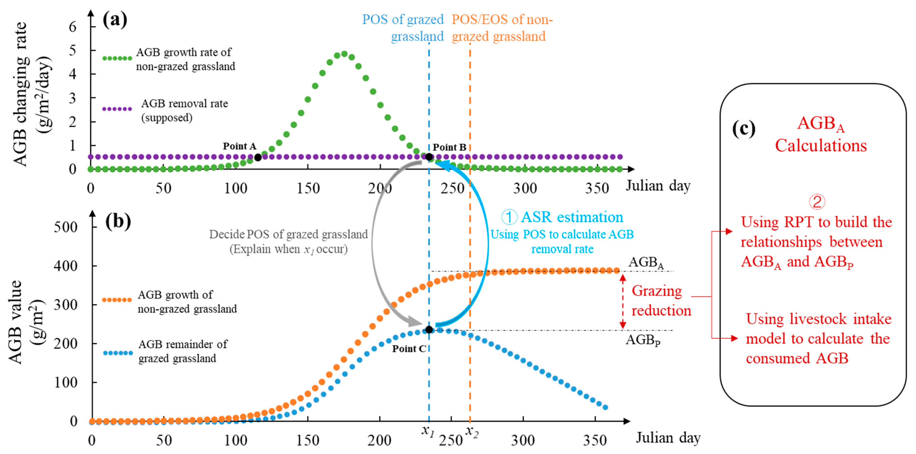
The theoretical models for estimating AGBA and ASR are delineated in Figure 1. Figure 1a illustrates the respective trendlines for the growth rate of AGB in non-grazed grassland (green) and the AGB removal rate (purple) due to livestock grazing. Figure 1b presents a comparative analysis of two trendlines, AGB growth of non-grazed grassland (orange) and AGB remainder of grazed grassland (blue), illustrating the commonly ignored consumed AGB caused by livestock (explanations displayed in Figure 1).
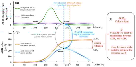
Figure 1.
Modelling theory of AGBA correction and ASR estimation (Subfigure (a) is the curve of AGB changing rate, subfigure (b) is the curve of AGB accumulation, subfigure (c) is AGBA calculation methods).
The key connection between Figure 1a,b is POS (x1 and x2), which links Point B and Point C. In scenarios where grassland undergoes grazing in Figure 1a, Point B, one of the point of intersections between these two trendlines, signifies an equilibrium where the AGB growth rate is equivalent to the AGB removal rate. Beyond this intersection, the growth rate subsequently falls behind the removal rate. Consequently, in Figure 1b, the peak of AGB for the grazed grassland is attained at the juncture marked by Point C, which correlates to the POS (x1) for the grazed grassland (Figure 1b). The path from Point B to Point C in Figure 1 explicates the methodology for deciding the POS (x1) in a grazed grassland context. This process explains the underlying mechanisms to determine when x1 occurs. Inversely, the POS of grazed grassland can be employed to calculate the AGB removal rate by the path from Point C to Point B (① in Figure 1b), thereby serving as an indirect measure of the stocking rate.
Figure 1c shows two methods used to improve AGBA and LCC estimation. The first one uses RPT derived from remote sensing images to build the relationships between AGBA and AGBP (② in Figure 1c). The second one employs a livestock intake model to calculate the consumed AGB if the livestock stocking rate is applicable. Our primary focus in this paper is on the first method, exploring the potential of RPT to enhance AGBA estimation.
As seasonal grazing is generally used in alpine grasslands, we evaluate the effectiveness of the modelling methods with and without the consideration of rotational grazing regimes. While the above modelling process is based on an assumption of pastures without seasonal rotational grazing regimes, it still works in a seasonal rotational grazed pastures for the growing season.
3.2. Overall Workflow
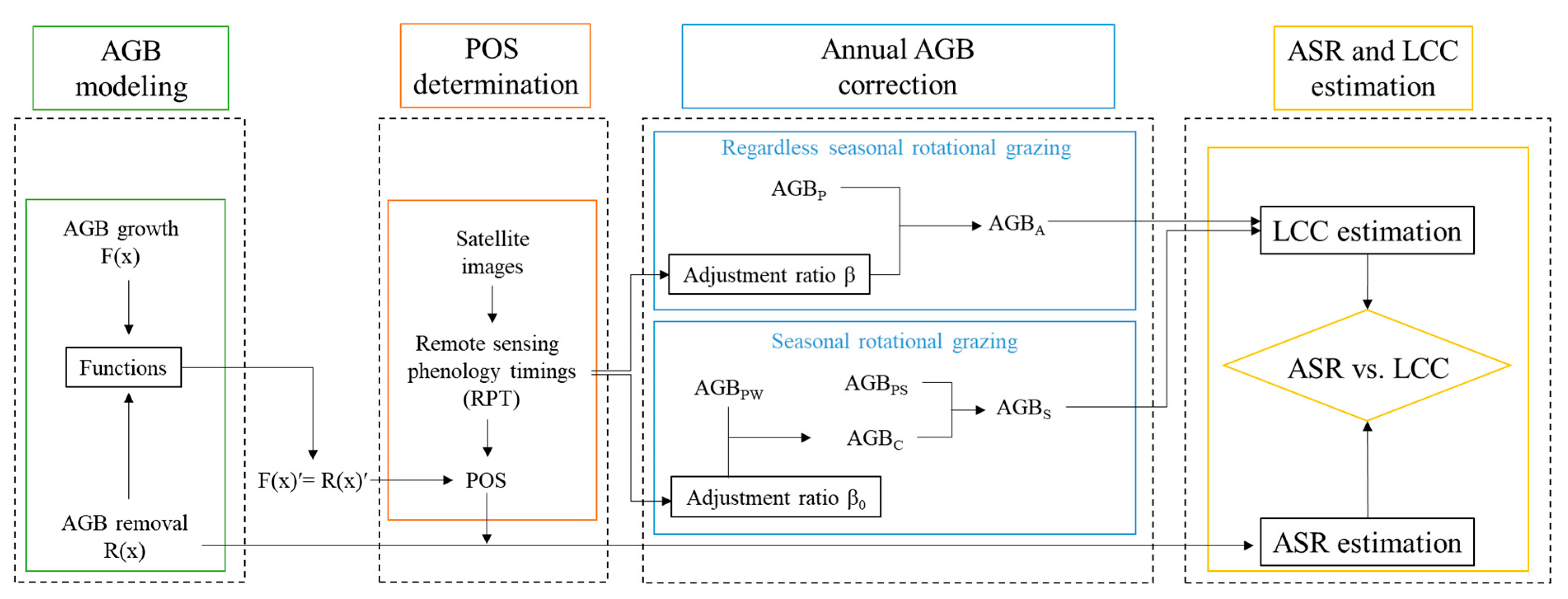
The workflow for estimating AGBP, LCC, and ASR based on remote sensing phenology timings has four main steps (Figure 2): (1) AGB modelling (including AGB growth and consumption models), (2) POS determination, (3) the correction of annual AGB estimation, and (4) LCC and ASR estimation and comparison. All the abbreviations in this study are listed in Table S2 and the Abbreviation Section.
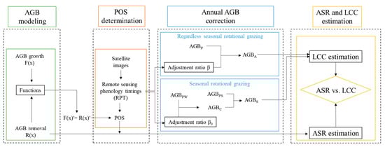
Figure 2.
A framework for LCC and ASR estimation. F(x) is the AGB growth function, F(x)′ refers to AGB growth rate. R(x) and R(x)′ are functions of AGB removal and removal rate, AGBPW is the peak above ground biomass of winter pasture, AGBPS the peak above ground biomass of summer pasture, AGBC is the plant biomass consumed by livestock in growing season, LCC is livestock carrying capacity, and ASR is the actual stocking rate.
First, we introduce models of AGB growth F(x) (in the condition of grazing exclusion) and AGB removal R(x) (consumption by livestock) to explain the underlying mechanisms between AGB accumulation and consumption. Second, the determination of POS is a priority to accurately estimate the AGBP. On one hand, phenological parameters including SOS, POS, EOS, and the length of the growing season can be determined using a smoothed VI time series [35]. On the other hand, POS can be calculated through functions representing AGB growth rate and AGB removal rate (Figure 1). This study focuses solely on the latter, as the former has been extensively researched and is widely documented in the existing literature [26,36]. Third, we propose two adjustment ratios, β0 and β, to characterize relations between peak and annual above ground biomass for situations with and without rotational grazing, respectively. The basis for these adjustment ratios is derived from the theory of AGB growth and consumption, as AGBP is not necessarily representative of AGBA in the context of grazed grasslands. Fourth, a comparative analysis between ASR and LCC is used to evaluate the grazing pressure on grassland ecosystems.
3.2.1. AGB Modelling
In alpine grassland, changes in AGB can be represented by a logistic function with three parameters [37,38], expressed as:
where: F(x) is the AGB growth representing the remaining AGB on the ground in the non-grazed grassland; F(x)′ is the derivative of F(x) and is the AGB growth rate. x is the Julian date. AGBmax is the maximum AGB by the day of EOS, which is the peak AGB in non-grazed grassland. X is the day (FOS) with the fastest growth rate; k is the standardized AGB growth rate (dividing the fastest AGB growth rate by AGBmax).
The AGB removal function refers to the daily consumption of AGB by livestock, and can be expressed as a linear function:
where R(x)′ is the AGB removal rate, which is a constant; 365 represents 365 days.
3.2.2. The Determination of POS
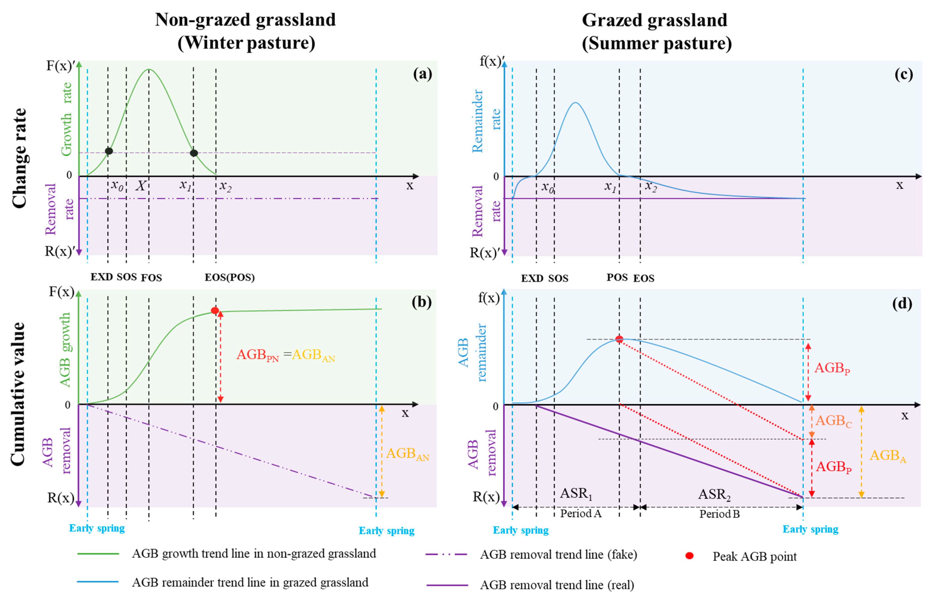
Figure 3 presents a schematic illustration of the AGB cumulative value and its change rate in grazed and non-grazed grasslands, showing the relationships between AGB and RPT. It is worth noting that the remote sensing detected phonology timings may slightly earlier than the ground observations; it should be considered in the algorithms.
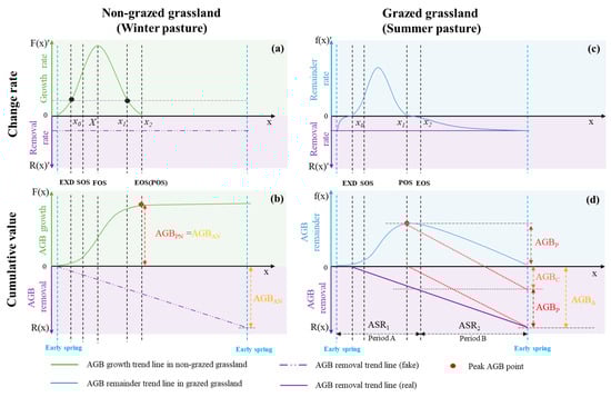
Figure 3.
Schematic illustration of AGB production and consumption (Subfigures (a,c) are AGB changing rate curve in non-grazed and grazed grassland, respectively. Subfigures (b,d) are AGB accumulation curves in non-grazed and grazed grassland, respectively.). AGBAN and AGBPN are for non-grazed grassland (or winter pasture); AGBA and AGBP are for grazed grassland (or summer pasture). F(x) is the AGB growth representing the remaining AGB in the non-grazed grassland; F(x)′ refers to AGB growth rate. f(x) represents the remainder AGB in the grazed grassland; f(x)′ refers to AGB remainder rate. R(x) and R(x)′ are AGB removal and removal rate. X is the day with the fastest growth rate (FOS) in the grazed grassland; x0 (EXD) is the day when F(x)′ exceed R(x)′; x1 is the day when F(x)′ lagged behind R(x)′).
In non-grazed grassland, AGBP occurs at the end of the grazing season, so in those settings, the POS is the same as the EOS in the Julian day (Figure 3b). The AGB growth rate, F(x)′, for non-grazed grassland, is simply the plant growth rate, but the AGB accumulation rate f(x)′ for grazed grassland is the joint effect of plant growth and livestock consumption (Figure 3d). Obviously, POS occurs before EOS in the grazed grassland, and it occurs when the AGB growth rate of non-grazed grassland (F(x)′) is equal to the AGB removal rate (R(x)′), just before the end of the growing season; this time point is displayed as x1 in Figure 3a. Thus, POS (x1) and EXD (x0) can be derived by the cross point of F(x)′ and R(x)′ as:
where F(x)″ < 0 secures the second point of the intersections of F(x)′ and R(x)′. It is noteworthy that at the juncture denoted by x0, the AGB growth rate F(x)′, surpasses the AGB removal rate R(x)′, whereas, at x1, the AGB growth rate F(x)′ lags behind the AGB removal rate R(x)′. In other words, f(x0)′ and f(x1)′ are zero, as shown in Figure 3d.
3.2.3. Annual AGB Correction
In ungrazed grassland (Figure 3c,d), AGB growth rate peaks at the end of the growing season:
where F(x)′ = 0 secures the extreme and F(x)″ < 0 ensures the POS (EOS).
Similarly, the peak biomass for the grazed grassland can be derived as (Figure 3c,d):
where f(x)′ = 0 secures the extremes and f(x)″ < 0 ensures the POS (x1).
The situation in the grazed grassland is more complex, due to the effects of livestock on the biomass dynamics of the system. AGBP is generally estimated through remotely sensed images obtained around the POS; it can be regarded as the forage storage used to feed livestock in dormant season (period B), which is the period after POS until growing re-commences, as shown in Figure 3d. Thus, AGBA includes AGBP and AGBC:
where: AGBC is the plant biomass consumed by livestock in growing season (period A), during which biomass is accumulating. It is worth noting that if AGB is in shortage or plenty by the end of winter season, the forage supplementary and the remanent biomass should be added and deducted in Equation (11), respectively.
Based on the concept outlined in Figure 3d, AGBC and AGBP can be used to calculate livestock carrying capacity for the period A and B, respectively (Figure 3):
where ASR1 and ASR2 stand for the actual stocking rate of periods A and B, respectively. Rs is a ratio including biomass use efficiency, availability, and edibility; it is assigned a value of 0.456 according to previous studies [39,40]. L is the daily intake for a standard sheep unit (SU), it is 1.8 kg/SU (NY/T635-2015) [41].
Theoretically, some livestock would be slaughtered after the growing season (regardless of the birth and death rates throughout the year). The actual stocking rate for the two periods (period A and B) can be described as Equation (14). Thus, the relationship between AGBA and AGBP can be derived from Equations (11)–(14):
where Srate is slaughter rate, and β is the adjustment ratio needed to convert AGBP to AGBA for the grazed grassland, assuming that grasslands were grazed in the same place across the year.
3.2.4. LCC and ASR Estimation
According to the definition and Equation (15), the annual LCC can be expressed as:
According to Equations (5) and (6), the POS is determined by F(x) (AGB growth of non-grazed grassland) and R(x) (the AGB removal function). With converse thinking, the POS can also reflect important information regarding plant growth (F(x)) and livestock grazing (R(x)). The ASR can be calculated by two steps. First, deriving the POS from VI time series data of the grazed grassland, and then assigning this POS(x1) to F(x)′ (AGB growth rate of non-grazed grassland) to calculate R(x)′ (the AGB removal rate). So, ASR can be expressed as:
where ASR is the actual stocking rate by the time of POS.
3.3. Model Application in Seasonal Rotational Grazing Regimes
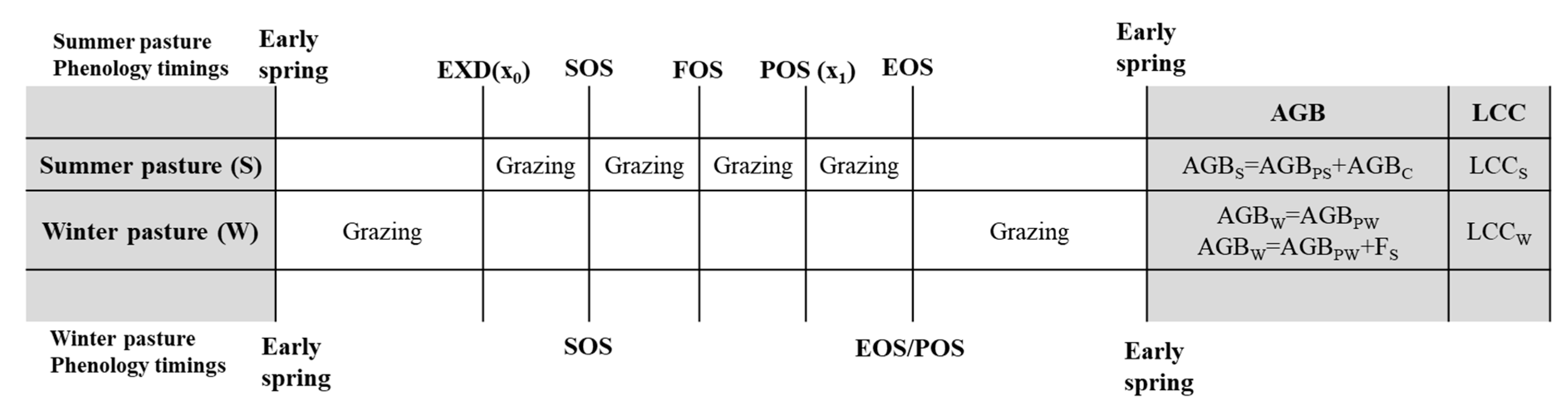
In theoretical terms, EXD and EOS in Figure 3a denote the optimal timing for the translocation of livestock between winter and summer pastures (see Figure 4). The temporal interval spanning from EXD to EOS signifies a state of abundance in AGB, whereas the days falling outside this temporal range are characterized by a scarcity of AGB. Grazing of summer pastures extends from EXD to EOS while livestock stay at winter pasture at other times of a year.
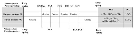
Figure 4.
Grazing status for summer and winter pastures at different phenology timings (AGBS is the total produced AGB on summer pasture; AGBW is the total demanded AGB for livestock on winter pasture; AGBPS and AGBPW represent AGBP for summer pasture and winter pasture, respectively. LCCS and LCCW represent LCC for summer pasture and winter pasture, respectively).
Thus, the calculation of AGBS should include AGBPS (the peak biomass of summer pasture) and AGBC (livestock consumed biomass). So, AGBS can be described as:
In winter pastures, AGBPW is produced in the summer season, and it is consumed in the winter season. The incorporation of FS (Forage Supplement) becomes imperative due to the diminished quality of AGB throughout the winter season. So, AGBW can be expressed as:
Based on the grazing status for a year displayed in Figure 4, the stocking rate in two pastures can be expressed as:
ASRS is the actual stocking rate for summer pasture, ASRW is the actual stocking rate for winter pasture, and Srate is the slaughter rate.
During the winter season, there is an observed decline in the crude protein content of the grasses from the summer season, which decreases notably from 10.43% to 5.56% [42]. So, the forage quality declined to 53.3% (Q) of the original (calculated by 5.56%/10.43%) based on the protein content. According to Equations (22)–(24), AGBC can be expressed as:
where β0 is the adjustment factor for calculating AGBC by the time of the POS in summer pasture based on AGBW. So, AGBS can be expressed as:
So, the livestock carrying capacity for two kinds of pastures can be expressed as:
where LCCS and LCCW represent the LCC for summer pasture and winter pasture, respectively. The determination of grassland carrying capacity is contingent upon the manner of utilization. For a grassland household with one summer pasture and one winter pasture, the best stocking rate during the summer season should be LCCS, and it should be reduced to LCCW during the winter season.
The expression of ASR at the time of the POS within the summer pasture can be derived in a similar manner to use of Equations (18) and (19).
3.4. Case Study
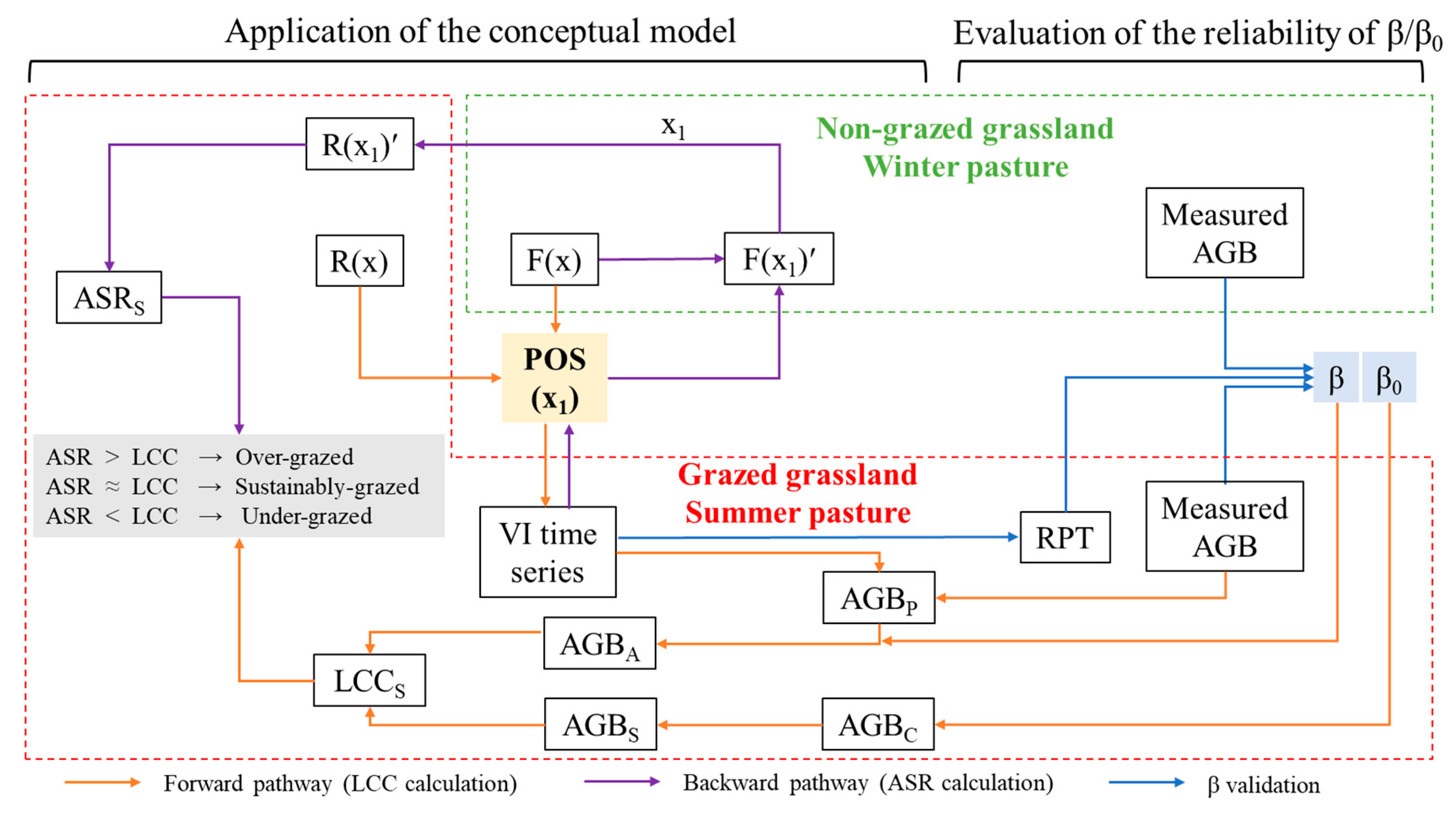
Figure 5 shows the workflow of the case study to test and validate the proposed models based on data derived from previously published papers (see Tables S1 and S2). The flow chart includes two parts; one is ‘Evaluation of the reliability of β/β0′ and the other one is ‘Application of the conceptual model’. The reliability of β was evaluated and validation of β draws on field-measured biomass and estimated RPT based on Equations (16) and (17) (blue arrows in Figure 5). Unfortunately, we are unable to evaluate β0 in this study due to the lack of data (controlled experiments).
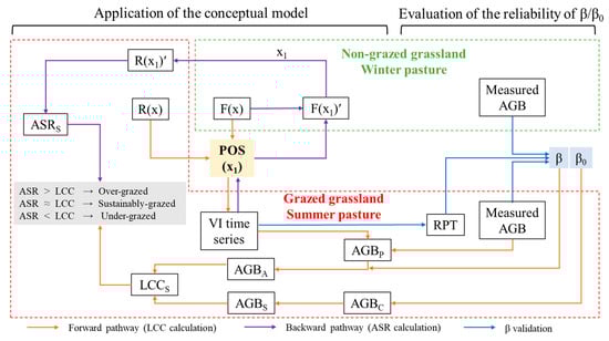
Figure 5.
Flow chart of the case study. F(x) is AGB growth function, F(x)′ is AGB growth rate function, R(x) is AGB removal function, R(x)′ is AGB removal rate function, and x1 is the day of POS in the grazed grassland.
The conceptual models start with the POS and then, via backward and forward pathways, we estimate the ASRS and LCCS, respectively. Comparison of the ASRS and LCCS indicates grassland grazing pressure: ASR > LCC means grassland is over-grazed, ASR ≈ LCC means grassland is grazed at a sustainable level, and ASR < LCC means grassland is grazed at a level lower than it could be. This conceptual model was applied to pastures with seasonal rotational grazing regimes to evaluate the grassland grazing pressure.
4. Results
4.1. The Reliability of β
Based on Equation (16), the value of β was estimated in two ways. The first approach is based on a meta-analysis of prior studies (Table 1), which involved estimating β through the use of phenological timings derived from VI time series images classified by vegetation type, covering alpine grasslands in QTP and Inner Mongolia from 1982 to 2016. Across these studies, the average value of β was derived as 1.47 ± 0.10 (mean ± SD).

Table 1.
Statistical summary of the phenological timings information used to calculate β.
The second approach calculated β using biomass data collected from non-grazed and grazed plot experiments (Table 2). In these studies, the non-grazed grassland areas were those where fencing had been established to exclude livestock and the grazed grassland was open to free grazing animals (at an unknown grazing intensity). The average value of β obtained through this approach was 1.45 ± 0.11 (mean ± SD). That both approaches yielded remarkably similar values of β confirms the accuracy of Equations (11)–(15) and highlights the strong coupling between AGBA and AGBP and phenological timing, regardless of the grazing intensity. Thus, on average, AGBA is about 1.45–1.47 larger than AGBP. Similarly, estimates of LCC based on AGBP are underestimated by about 31% (0.45/1.45 to 0.47/1.47).
Table 2.
Statistical summary of the field measurements of AGB in plot experiments used to calculate β.
4.2. The Estimation of LCC and ASR
The estimation of LCCS and ASRS is based on the mechanisms displayed in Figure 3. The POS was determined by the joint effects of plant growth and grazing activity [30,49]. Conversely, the POS can be used to reflect the grazing severity through plant growth function as shown in Equations (18) and (19). The data used to estimate the LCCS and the ASRS were taken from the same place to ensure a similar plant growth function under similar ecological and environmental conditions. These studies were carried out in the alpine grasslands in Haibei alpine meadow, Qinghai, China (Table 3). The value of the variables is averaged corresponding to their observation periods. The RPT variables were observed from the study of Zhu, Zhang [43]. Moreover, the peak AGB estimated by remote sensing for summer pastures is varied, so the mean value was used in the model (Table 3).
Table 3.
Description of variables used in the model application.
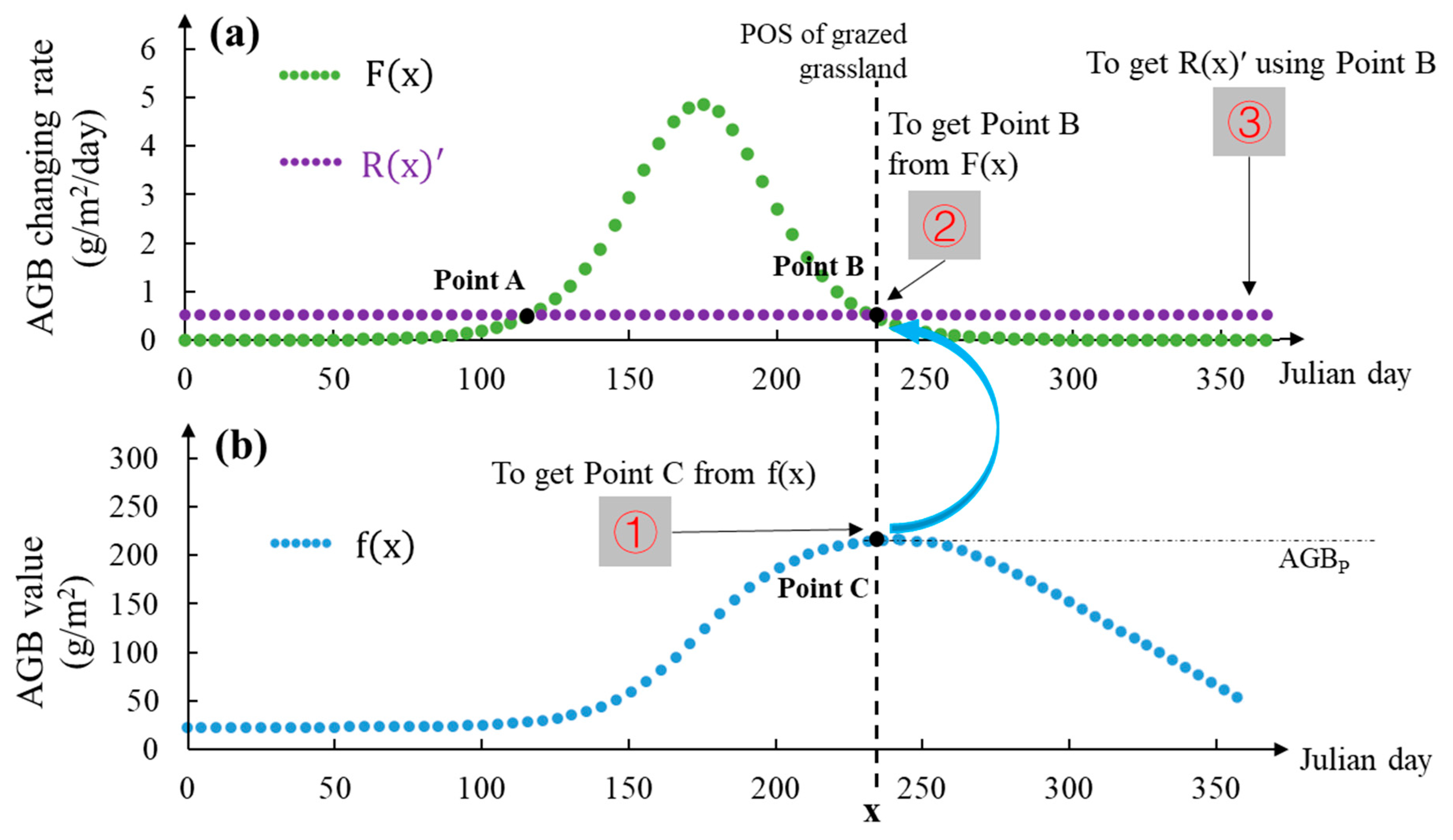
The plant growth rate model (Equation (30) is from Equation (2)) was implemented based on the study of Wang, Liu [37]. Figure 6 shows a simplified workflow using the POS to calculate AGB removal rate based on Figure 1. After the POS (x1, in grazed grassland) was derived from remote sensing images (step ①), it was used to calculate the AGB removal rate (R(x)′) via Point B (step ② and ③).
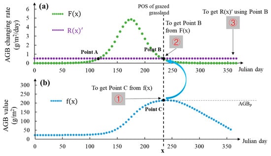
Figure 6.
Illustration of using POS to calculate AGB removal rate ((a) simplified workflow of Figure 1, ①–③ are three steps. Subfigure a is the curve of AGB changing rate, subfigure (b) is the curve of AGB accumulation).
The results displayed in Table 4, which calculate EXD(x0) and β0 from observations in Table 3, were 131 Julian day and 0.434, respectively. Based on these two important factors, the ASR and LCC can be derived. The ASRS was 2.91 SU/ha and the LCCS was 2.61 SU/ha. Thus, it appears that the summer pastures in Haibei alpine grassland were averagely over-stocked by 11.5% in the period from 2000 to 2005. Prospectively, methods outlined here to evaluate grazing pressure using phenology timings based on remote sensing imagery using a plant growth model could provide a solution to map the dynamics of grazing activities for large-scale studies.
Table 4.
Comparison of modelling results.
5. Discussion
Accurate prediction of ASR and LCC is key to determinations of grazing pressure that underpin interpretations of successful livestock management [6]. Prospects for sustainable grazing reflect the balance between land-use practices (especially stocking rates and rotational grazing practices) and grassland productivity [55]. Estimation of the ASR and LCC via remote sensing requires an understanding of biomass growth and consumption mechanisms [6,26,30]. Findings from this study show the reliability and effectiveness of two ratios, β and β0, which link AGBP and AGBC to AGBA. These results enhance the utility of the models presented in Figure 1, highlighting the importance of phenological timings in the estimation of the ASR and LCC.
Traditional models that do not incorporate spatial and temporal variability in forage production [25] or knowledge of seasonal grazing patterns [56] are likely to overestimate the AGBA and LCC. Conversely, utilizing the AGBP instead of the AGBA likely underestimates the LCC. For averaged values in the large-scale studies of alpine grassland on QTP, our results indicate that the LCC, estimated based on the AGBP, is underestimated by about 31% due to the difference between the AGBP and the AGBA (β). This explains why previous studies that use the AGBP as a proxy for the AGBA have yielded inconsistent results for the same area over the same period (Table S1). Although ground truth data can be measured in non-grazed grassland, as most areas on the QTP are grazed, using only non-grazed information causes errors in spatial analyses of biomass and productivity. Furthermore, while most studies have collected ground truth data in grazed grassland (Table S1), what is stated to be the annual AGB is actually the peak biomass. In any case, the proposed adjustment ratio β can be used to avoid underestimation of the LCC for the pastures with and without the consideration of rotational grazing regimes. This exemplifies the critical importance of underlying assumptions and analytical procedures in using automated procedures [57].
Determining and implementing an appropriate grazing intensity and ASR is key to the sustainable management of grassland resources [58]. An excessively high stocking rate may cause land degradation and desertification [59], whereas appropriately managed grazing (e.g., rotational grazing regimes) can contribute to the provision of ecosystem services [60]. In this study, the grazing pressure was evaluated by using phenology timings derived from remote sensing images with the assistance of a plant growth model. The results indicate that the summer pastures in Haibei alpine grassland were, averagely, over-stocked by 11.5% in the period of 2000–2005. The ability of remote sensing phenological timings to estimate the ASR provides a solution to map the spatial dynamic of grazing activities, such as stocking rate and grazing intensity. However, multiple plant growth models are required to conduct such large-scale mapping studies.
Livestock grazing and plant growth alter biomass dynamics and determine POS in tandem. In some instances, more productive plant communities in free-grazing alpine grasslands reach their POS later than less-productive plant communities [9]. Hence, parameterization (and structure) of plant community growth models will likely need to vary from place to place to reflect local conditions in plant composition and the environment [38,61]. For example, it has been argued that the stocking rate should be estimated for different topographic positions, as topography (e.g., aspect) controls biomass and its availability to livestock [61,62]. Given the sharply changing rate of F(x)′ (plant growth rate) displayed in Figure 5, R(x)′ (relevant to ASR and x0), it is critical to accurately estimate the POS. Observations and analyses of specific plant community growth models and remote sensing phenology are required to support reliable transfer of LCC predictions in space and across scales. Accurate determination of the POS can help to predict appropriate grazing intensity or stocking rate, thereby supporting livestock producers and land managers alike. Additionally, to integrate remotely sensed timings with the plant growth model, the remotely sensed timing data were utilized as average values for the study area, represented in vector format rather than raster data. This decision was made due to the challenges associated with transferring the plant growth model into raster format. However, employing a patch-based analysis approach, supported by multiple plant growth models representing various community or vegetation types, could facilitate the estimation of ASR across extensive spatial extents. The availability of high-resolution and high-frequency satellite imageries, such as Sentinel 2 and Planet Scope satellites, now provides strong foundations to support applications of the procedures outlined in this study.
6. Conclusions
This study evaluated, for the first time, the underlying mechanisms between remote sensing phenology and grazing activity. The evidence provided highlights the importance of the relationships between the AGBP, AGBC, and AGBA, and associated implications for the determination of the ASR and LCC. We present a new approach based upon phenological timings of plant growth models to support such tasks. A statistical method based on the relationships between the AGBP, AGBC, and AGBA is used to derive adjustment ratios based on remote sensing phenology timings. The reliability of these ratios and the feasibility of the proposed models were corroborated and tested by observations from previous studies. Our novel method uses remote sensing phenology timings to estimate the ASR based on plant growth models in a backward pathway. Estimates of the LCC based on remote-sensed biomass are adjusted by β and β0 for different scale studies. Our method efficiently tracks the stocking rate and predicts the carrying capacity, thereby supporting sustainable grazing strategies in alpine grasslands.
Supplementary Materials
The following supporting information can be downloaded at: https://www.mdpi.com/article/10.3390/rs16111991/s1. Refs. [63,64,65,66] are cited in the Supplementary Materials.
Author Contributions
Y.S. conceived the ideas and designed methodology; G.B. contributed to the conception and the original draft. Y.S. led the writing of the manuscript with contributions from G.L.W.P., J.G., X.L., A.V.P., M.H. and J.L. All authors have read and agreed to the published version of the manuscript.
Funding
This research was funded by the China Postdoctoral Science Foundation (GZC20230998), the National Natural Science Foundation of China (U23A20159), the Opening Foundation of Key Laboratory of the Alpine Grassland Ecology in the Three River Region, Ministry of Education (2023-SJY-KF-05) and Discipline Innovation and Introducing Talents Program of Higher Education Institutions (D18013).
Data Availability Statement
Data are already published and publicly available, with those items properly cited in this submission. Data [37] are available from Figshare: https://doi.org/10.6084/m9.figshare.11663997, while other data is presented in the tables within this manuscript.
Conflicts of Interest
The authors have no conflicts of interest.
Abbreviations
Note: the unit of F(x) and R(x) is g/m2, and their derivative is g/m2/day, the unit of LCC and ASR are SU/ha
| Abbreviation | Meaning |
| AGBA | Annual above ground biomass (grazed grassland) |
| AGBP | Peak above ground biomass (grazed grassland) |
| AGBAN | Annual above ground biomass (non-grazed grassland) |
| AGBPN | Peak above ground biomass (non-grazed grassland) |
| AGBC | The plant biomass consumed by livestock in growing season (by the time of POS in summer pasture) |
| AGBS | Total produced above ground biomass on summer pasture |
| AGBW | Total demanded above ground biomass for livestock on winter pasture |
| AGBPS | Peak above ground biomass of summer pasture (the AGB remainder) |
| AGBPW | Peak above ground biomass of winter pasture (the AGB remainder) |
| Rs | The ratios including biomass use efficiency, availability, and edibility |
| L | The daily intake for a standard sheep unit (SU) |
| β | The adjustment ratio to convert AGBP to AGBA for the grazed grassland (regardless rotational regimes) |
| β0 | The adjustment ratio for calculating AGBC based on AGBW (for rotational grazing regimes) |
| k | The standardized fastest AGB growth rate |
| Srate | Slaughter rate (at the end of growing season) |
| RPT | Remote sensing phenology timings |
| LCC | Livestock carrying capacity |
| ASR | Actual stocking rate |
| ASRS | Actual stocking rate of summer pasture |
| ASRW | Actual stocking rate of winter pasture |
| LCC1 | Livestock carrying capacity for period A |
| LCC2 | Livestock carrying capacity for period B |
| LCCS | Livestock carrying capacity of summer pasture |
| LCCW | Livestock carrying capacity of winter pasture |
| EXD | The day of AGB growth rate F(x)ʹ exceed AGB removal rate R(x)ʹ |
| POS | The peak of the growing season (remote sensing phonology) |
| EOS | The end of the growing season (remote sensing phonology) |
| SOS | The start of the growing season (remote sensing phonology) |
| FOS | The day having the fastest growth rate |
| x0 | The day of EXD in the grazed grassland |
| x1 | The day of POS in the grazed grassland |
| x2 | The day of POS in the non-grazed grassland (POS and EOS are the same day) |
| X | The day having the fastest growth rate (FOS) in the grazed grassland |
| Period A | The period from Early spring to POS (biomass accumulating period) |
| Period B | The period from POS to the next Early spring (the period after POS until growing resumes) |
| F(x) | AGB growth function representing the remaining AGB in the non-grazed grassland |
| F(x)′ | AGB growth rate in the non-grazed grassland |
| R(x) | AGB removal function representing the consumed AGB |
| R(x)′ | AGB removal rate |
| f(x) | AGB accumulation representing the remaining AGB in the grazed grassland |
References
- Bardgett, R.D.; Bullock, J.M.; Lavorel, S.; Manning, P.; Schaffner, U.; Ostle, N.; Chomel, M.; Durigan, G.; Fry, E.L.; Johnson, D.; et al. Combatting global grassland degradation. Nat. Rev. Earth Environ. 2021, 2, 720–735. [Google Scholar] [CrossRef]
- Yuan, Q.; Yuan, Q.; Ren, P. Coupled effect of climate change and human activities on the restoration/degradation of the Qinghai-Tibet Plateau grassland. J. Geogr. Sci. 2021, 31, 1299–1327. [Google Scholar] [CrossRef]
- Harris, R.B. Rangeland degradation on the Qinghai-Tibetan plateau: A review of the evidence of its magnitude and causes. J. Arid Environ. 2010, 74, 1–12. [Google Scholar] [CrossRef]
- Luo, T.; Li, W.; Zhu, H. Estimated biomass and productivity of natural vegetation on the Tibetan Plateau. Ecol. Appl. 2002, 12, 980–997. [Google Scholar] [CrossRef]
- Yang, Y.; Zhao, D.; Chen, H. Full Title: Quantifying the ecological carrying capacity of alpine grasslands on the Qinghai-Tibet Plateau. Ecol. Indic. 2022, 136, 108634. [Google Scholar] [CrossRef]
- Piipponen, J.; Jalava, M.; de Leeuw, J.; Rizayeva, A.; Godde, C.; Cramer, G.; Herrero, M.; Kummu, M. Global trends in grassland carrying capacity and relative stocking density of livestock. Glob. Chang. Biol. 2022, 28, 3902–3919. [Google Scholar] [CrossRef] [PubMed]
- Shi, Y.; Gao, J.; Li, X.; Brierley, G.; Lin, C.; Ma, X. Spatiotemporal Variability of Alpine Meadow Aboveground Biomass and Sustainable Grazing in Light of Climate Warming. Rangel. Ecol. Manag. 2023, 90, 64–77. [Google Scholar] [CrossRef]
- Wang, H.; Liu, H.; Huang, N.; Bi, J.; Ma, X.; Ma, Z.; Shangguan, Z.; Zhao, H.; Feng, Q.; Liang, T.; et al. Satellite-derived NDVI underestimates the advancement of alpine vegetation growth over the past three decades. Ecology 2021, 102, e03518. [Google Scholar] [CrossRef] [PubMed]
- Duparc, A.; Redjadj, C.; Viard-Crétat, F.; Lavorel, S.; Austrheim, G.; Loison, A. Co-variation between plant above-ground biomass and phenology in sub-alpine grasslands. Appl. Veg. Sci. 2013, 16, 305–316. [Google Scholar] [CrossRef]
- Oesterheld, M.; Sala, O.E.; McNaughton, S.J. Effect of animal husbandry on herbivore-carrying capacity at a regional scale. Nature 1992, 356, 234–236. [Google Scholar] [CrossRef]
- Zhang, J.; Zhang, L.; Liu, W.; Qi, Y.; Wo, X. Livestock-carrying capacity and overgrazing status of alpine grassland in the Three-River Headwaters region, China. J. Geogr. Sci. 2014, 24, 303–312. [Google Scholar] [CrossRef]
- Cao, Y.; Wu, J.; Zhang, X.; Niu, B.; Li, M.; Zhang, Y.; Wang, X.; Wang, Z. Dynamic forage-livestock balance analysis in alpine grasslands on the Northern Tibetan Plateau. J. Environ. Manag. 2019, 238, 352–359. [Google Scholar] [CrossRef] [PubMed]
- Retzer, V.; Reudenbach, C. Modelling the carrying capacity and coexistence of pika and livestock in the mountain steppe of the South Gobi, Mongolia. Ecol. Model. 2005, 189, 89–104. [Google Scholar] [CrossRef]
- Zhang, J.; Zhang, L.; Liu, X.; Qiao, Q. Research on sustainable development in an alpine pastoral area based on equilibrium analysis between the grassland yield, livestock carrying capacity, and animal husbandry population. Sustainably 2019, 11, 4659. [Google Scholar] [CrossRef]
- Zhang, X.; Li, M.; Wu, J.; He, Y.; Niu, B. Alpine Grassland Aboveground Biomass and Theoretical Livestock Carrying Capacity on the Tibetan Plateau. J. Resour. Ecol. 2022, 13, 129–141. [Google Scholar] [CrossRef]
- Yang, S.X.; Feng, Q.S.; Liang, T.G.; Liu, B.K.; Zhang, W.J.; Xie, H.J. Modeling grassland above-ground biomass based on artificial neural network and remote sensing in the Three-River Headwaters Region. Remote Sens. Environ. 2018, 204, 448–455. [Google Scholar] [CrossRef]
- Zhang, J.; Fang, S.; Liu, H. Estimation of alpine grassland above-ground biomass and its response to climate on the Qinghai-Tibet Plateau during 2001 to 2019. Glob. Ecol. Conserv. 2022, 35, e02065. [Google Scholar] [CrossRef]
- Scurlock, J.M.; Johnson, K.; Olson, R.J. Estimating net primary productivity from grassland biomass dynamics measurements. Glob. Chang. Biol. 2002, 8, 736–753. [Google Scholar] [CrossRef]
- Mo, X.G.; Liu, W.; Meng, C.C.; Hu, S.; Liu, S.X.; Lin, Z.H. Variations of forage yield and forage-livestock balance in grasslands over the Tibetan Plateau, China. Chin. J. Appl. Ecol. 2021, 32, 2415–2425. [Google Scholar] [CrossRef]
- Liu, H.; Mi, Z.; Lin, L.; Wang, Y.; Zhang, Z.; Zhang, F.; Wang, H.; Liu, L.; Zhu, B.; Cao, G.; et al. Shifting plant species composition in response to climate change stabilizes grassland primary production. Proc. Natl. Acad. Sci. USA 2018, 115, 4051–4056. [Google Scholar] [CrossRef]
- Qin, P.; Sun, B.; Li, Z.; Gao, Z.; Li, Y.; Yan, Z.; Gao, T. Estimation of grassland carrying capacity by applying high spatiotemporal remote sensing techniques in Zhenglan Banner, Inner Mongolia, China. Sustainability 2021, 13, 3123. [Google Scholar] [CrossRef]
- Ping, W.; Zhiwei, W.; Xuetong, Z.; Qisheng, F.; Cili, J.; Quangong, C. GIS-based classification of seasonal pasture in Qinghai province. Pratacultural Sci. 2010, 27, 119–128. [Google Scholar]
- Wei, D.; Zhao, H.; Zhang, J.; Qi, Y.; Wang, X. Human activities alter response of alpine grasslands on Tibetan Plateau to climate change. J. Environ. Manag. 2020, 262, 110335. [Google Scholar] [CrossRef] [PubMed]
- Wang, X.; Li, F.Y.; Tang, K.; Wang, Y.; Suri, G.; Bai, Z.; Baoyin, T. Land use alters relationships of grassland productivity with plant and arthropod diversity in Inner Mongolian grassland. Ecol. Appl. 2020, 30, e02052. [Google Scholar] [CrossRef] [PubMed]
- Wang, Y.; Lv, W.; Xue, K.; Wang, S.; Zhang, L.; Hu, R.; Zeng, H.; Xu, X.; Li, Y.; Jiang, L.; et al. Grassland changes and adaptive management on the Qinghai–Tibetan Plateau. Nat. Rev. Earth Environ. 2022, 3, 668–683. [Google Scholar] [CrossRef]
- Song, Y.; Munch, S.B.; Zhu, K. Prediction-based approach for quantifying phenological mismatch across landscapes under climate change. Landsc. Ecol. 2023, 38, 821–845. [Google Scholar] [CrossRef]
- Möhl, P.; von Büren, R.S.; Hiltbrunner, E. Growth of alpine grassland will start and stop earlier under climate warming. Nat. Commun. 2022, 13, 7398. [Google Scholar] [CrossRef] [PubMed]
- Wu, M.; Vico, G.; Manzoni, S.; Cai, Z.; Bassiouni, M.; Tian, F.; Zhang, J.; Ye, K.; Messori, G. Early Growing Season Anomalies in Vegetation Activity Determine the Large-Scale Climate-Vegetation Coupling in Europe. J. Geophys. Res. Biogeosci. 2021, 126, e2020JG006167. [Google Scholar] [CrossRef]
- Richardson, W.; Stringham, T.K.; Lieurance, W.; Snyder, K.A. Changes in Meadow Phenology in Response to Grazing Management at Multiple Scales of Measurement. Remote Sens. 2021, 13, 4028. [Google Scholar] [CrossRef]
- Shen, M.; Wang, S.; Jiang, N.; Sun, J.; Cao, R.; Ling, X.; Fang, B.; Zhang, L.; Zhang, L.; Xu, X.; et al. Plant phenology changes and drivers on the Qinghai–Tibetan Plateau. Nat. Rev. Earth Environ. 2022, 3, 633–651. [Google Scholar] [CrossRef]
- Zhang, L.; Guo, H.; Jia, G.; Wylie, B.; Gilmanov, T.; Howard, D.; Ji, L.; Xiao, J.; Li, J.; Yuan, W.; et al. Net ecosystem productivity of temperate grasslands in northern China: An upscaling study. Agric. For. Meteorol. 2014, 184, 71–81. [Google Scholar] [CrossRef]
- Mao, D.; Wang, Z.; Li, L.; Ma, W. Spatiotemporal dynamics of grassland aboveground net primary productivity and its association with climatic pattern and changes in Northern China. Ecol. Indic. 2014, 41, 40–48. [Google Scholar] [CrossRef]
- Chai, Q.; Gan, Y.; Zhao, C.; Xu, H.-L.; Waskom, R.M.; Niu, Y.; Siddique, K.H.M. Regulated deficit irrigation for crop production under drought stress. A review. Agron. Sustain. Dev. 2015, 36, 3. [Google Scholar] [CrossRef]
- Deng, X.-P.; Shan, L.; Zhang, H.; Turner, N.C. Improving agricultural water use efficiency in arid and semiarid areas of China. Agric. Water Manag. 2006, 80, 23–40. [Google Scholar] [CrossRef]
- Xie, J.; Jonas, T.; Rixen, C.; de Jong, R.; Garonna, I.; Notarnicola, C.; Asam, S.; Schaepman, M.; Kneubühler, M. Land surface phenology and greenness in Alpine grasslands driven by seasonal snow and meteorological factors. Sci. Total Environ. 2020, 725, 138380. [Google Scholar] [CrossRef]
- Wang, J.; Zhou, T.; Peng, P. Phenology Response to Climatic Dynamic across China’s Grasslands from 1985 to 2010. ISPRS Int. J. Geo-Inf. 2018, 7, 290. [Google Scholar] [CrossRef]
- Wang, H.; Liu, H.; Cao, G.; Ma, Z.; Li, Y.; Zhang, F.; Zhao, X.; Zhao, X.; Jiang, L.; Sanders, N.J.; et al. Alpine grassland plants grow earlier and faster but biomass remains unchanged over 35 years of climate change. Ecol. Lett. 2020, 23, 701–710. [Google Scholar] [CrossRef]
- Huang, L.; Koubek, T.; Weiser, M.; Herben, T. Environmental drivers and phylogenetic constraints of growth phenologies across a large set of herbaceous species. J. Ecol. 2018, 106, 1621–1633. [Google Scholar] [CrossRef]
- Yu, L.; Zhou, L.; Liu, W.; Zhou, H.-K. Using Remote Sensing and GIS Technologies to Estimate Grass Yield and Livestock Carrying Capacity of Alpine Grasslands in Golog Prefecture, China. Pedosphere 2010, 20, 342–351. [Google Scholar] [CrossRef]
- He, F.; Chen, D.; Li, Q.; Chen, X.; Huo, L.; Zhao, L.; Zhao, X. Temporal and spatial distribution of herbage nutrition in alpine grassland of Sanjiangyuan. Acta Ecol. Sin. 2020, 40, 6304–6313. [Google Scholar] [CrossRef]
- Cao, Y.; Wu, J.; Zhang, X.; Niu, B.; He, Y. Comparison of Methods for Evaluating the Forage-Livestock Balance of Alpine Grasslands on the Northern Tibetan Plateau. J. Resour. Ecol. 2020, 11, 272–282. [Google Scholar] [CrossRef]
- Cai, Z.; Song, P.; Wang, J.; Jiang, F.; Liang, C.; Zhang, J.; Gao, H.; Zhang, T. Grazing pressure index considering both wildlife and livestock in Three-River Headwaters, Qinghai-Tibetan Plateau. Ecol. Indic. 2022, 143, 109338. [Google Scholar] [CrossRef]
- Zhu, Y.; Zhang, Y.; Zu, J.; Wang, Z.; Huang, K.; Cong, N.; Tang, Z. Effects of data temporal resolution on phenology extractions from the alpine grasslands of the Tibetan Plateau. Ecol. Indic. 2019, 104, 365–377. [Google Scholar] [CrossRef]
- Ding, M.J.; Zhang, Y.L.; Sun, X.M.; Liu, L.S.; Wang, Z.F.; Bai, W.Q. Spatiotemporal variation in alpine grassland phenology in the Qinghai-Tibetan Plateau from 1999 to 2009. Chin. Sci. Bull. 2013, 58, 396–405. [Google Scholar] [CrossRef]
- Yang, J.; Dong, J.; Xiao, X.; Dai, J.; Wu, C.; Xia, J.; Zhao, G.; Zhao, M.; Li, Z.; Zhang, Y.; et al. Divergent shifts in peak photosynthesis timing of temperate and alpine grasslands in China. Remote Sens. Environ. 2019, 233, 111395. [Google Scholar] [CrossRef]
- Zhang, C.; Zhang, Y.; Wang, Z.; Li, J.; Odeh, I. Monitoring Phenology in the Temperate Grasslands of China from 1982 to 2015 and Its Relation to Net Primary Productivity. Sustainability 2020, 12, 12. [Google Scholar] [CrossRef]
- Wu, J.; Zhang, X.; Shen, Z.; Shi, P.; Xu, X.; Li, X. Grazing-Exclusion Effects on Aboveground Biomass and Water-Use Efficiency of Alpine Grasslands on the Northern Tibetan Plateau. Rangel. Ecol. Manag. 2013, 66, 454–461. [Google Scholar] [CrossRef]
- Zhao, J.; Sun, F.; Tian, L. Altitudinal pattern of grazing exclusion effects on vegetation characteristics and soil properties in alpine grasslands on the central Tibetan Plateau. J. Soils Sediments 2019, 19, 750–761. [Google Scholar] [CrossRef]
- Hu, G.; Gao, Q.; Ganjurjav, H.; Wang, Z.; Luo, W.; Wu, H.; Li, Y.; Yan, Y.; Gornish, E.S.; Schwartz, M.W.; et al. The divergent impact of phenology change on the productivity of alpine grassland due to different timing of drought on the Tibetan Plateau. Land Degrad. Dev. 2021, 32, 4033–4041. [Google Scholar] [CrossRef]
- Li, W.; Ma, X.; Chen, Q. Research on grassland resources yield and balance between forage resources and livestock numbers in Haidong and Haibei prefecture of Qinghai. Acta Prataculturae Sin. 2009, 18, 270–275. [Google Scholar]
- Jia, W.X.; Liu, M.; Yang, Y.H.; He, H.L.; Zhu, X.D.; Yang, F.; Yin, C.; Xiang, W.N. Estimation and uncertainty analyses of grassland biomass in Northern China: Comparison of multiple remote sensing data sources and modeling approaches. Ecol. Indic. 2016, 60, 1031–1040. [Google Scholar] [CrossRef]
- Gao, X.X.; Dong, S.K.; Li, S.; Xu, Y.D.; Liu, S.L.; Zhao, H.D.; Yeomans, J.; Li, Y.; Shen, H.; Wu, S.N.; et al. Using the random forest model and validated MODIS with the field spectrometer measurement promote the accuracy of estimating aboveground biomass and coverage of alpine grasslands on the Qinghai-Tibetan Plateau. Ecol. Indic. 2020, 112, 106114. [Google Scholar] [CrossRef]
- Yu, H.; Wu, Y.; Niu, L.; Chai, Y.; Feng, Q.; Wang, W.; Liang, T. A method to avoid spatial overfitting in estimation of grassland above-ground biomass on the Tibetan Plateau. Ecol. Indic. 2021, 125, 107450. [Google Scholar] [CrossRef]
- Yang, Y.; Fang, J.; Pan, Y.; Ji, C. Aboveground biomass in Tibetan grasslands. J. Arid Environ. 2009, 73, 91–95. [Google Scholar] [CrossRef]
- Huang, W.; Bruemmer, B.; Huntsinger, L. Incorporating measures of grassland productivity into efficiency estimates for livestock grazing on the Qinghai-Tibetan Plateau in China. Ecol. Econ. 2016, 122, 1–11. [Google Scholar] [CrossRef]
- Briske, D.D.; Coppock, D.L.; Illius, A.W.; Fuhlendorf, S.D. Strategies for global rangeland stewardship: Assessment through the lens of the equilibrium–non-equilibrium debate. J. Appl. Ecol. 2020, 57, 1056–1067. [Google Scholar] [CrossRef]
- O’Neil, C. Weapons of Math Destruction: How Big Data Increases Inequality and Threatens Democracy; Crown: New York, NY, USA, 2017. [Google Scholar]
- Zhang, C.; Dong, Q.; Chu, H.; Shi, J.; Li, S.; Wang, Y.; Yang, X. Grassland Community Composition Response to Grazing Intensity Under Different Grazing Regimes. Rangel. Ecol. Manag. 2018, 71, 196–204. [Google Scholar] [CrossRef]
- Li, X.; Perry, G.L.W.; Brierley, G.J. A spatial simulation model to assess controls upon grassland degradation on the Qinghai-Tibet Plateau, China. Appl. Geogr. 2018, 98, 166–176. [Google Scholar] [CrossRef]
- Bengtsson, J.; Bullock, J.M.; Egoh, B.; Everson, C.; Everson, T.; O’Connor, T.; O’Farrell, P.J.; Smith, H.G.; Lindborg, R. Grasslands—More important for ecosystem services than you might think. Ecosphere 2019, 10, e02582. [Google Scholar] [CrossRef]
- Sanaei, A.; Li, M.; Ali, A. Topography, grazing, and soil textures control over rangelands’ vegetation quantity and quality. Sci. Total Environ. 2019, 697, 134153. [Google Scholar] [CrossRef]
- Hua, X.; Ohlemüller, R.; Sirguey, P. Differential effects of topography on the timing of the growing season in mountainous grassland ecosystems. Environ. Adv. 2022, 8, 100234. [Google Scholar] [CrossRef]
- Ma, A.; He, N.; Yu, G.; Wen, D.; Peng, S. Carbon storage in Chinese grassland ecosystems: Influence of different integrative methods. Sci. Rep. 2016, 6, 21378. [Google Scholar] [CrossRef] [PubMed]
- Ni, J. Carbon storage in terrestrial ecosystems of China: Estimates at different spatial resolutions and their responses to climate change. Clim. Change 2001, 49, 339–358. [Google Scholar] [CrossRef]
- Qu, Y.; Zhao, Y.; Ding, G.; Chi, W.; Gao, G. Spatiotemporal patterns of the forage-livestock balance in the Xilin Gol steppe, China: Implications for sustainably utilizing grassland-ecosystem services. J. Arid. Land 2021, 13, 135–151. [Google Scholar] [CrossRef]
- Zhang, F.; Wang, H.; Zhu, Y.; Zhang, Z.; Li, X. Study on the Aboveground Biomass of Natural Grassland and Balance between Forage and Livestock in Qilian County. J. Nat. Resour. 2017, 32, 1183–1192. [Google Scholar]
Disclaimer/Publisher’s Note: The statements, opinions and data contained in all publications are solely those of the individual author(s) and contributor(s) and not of MDPI and/or the editor(s). MDPI and/or the editor(s) disclaim responsibility for any injury to people or property resulting from any ideas, methods, instructions or products referred to in the content. |
© 2024 by the authors. Licensee MDPI, Basel, Switzerland. This article is an open access article distributed under the terms and conditions of the Creative Commons Attribution (CC BY) license (https://creativecommons.org/licenses/by/4.0/).