Mapping Topsoil Carbon Storage Dynamics of Croplands Based on Temporal Mosaicking Images of Landsat and Machine Learning Approach

Abstract

Understanding changes of soil organic carbon (SOC) in top layers of croplands and their driving factors is a vital prerequisite in decision-making for maintaining sustainable agriculture. However, high-precision estimation of SOC of croplands at regional scale is still an issue to be solved. Based on soil samples, synthetic image of bare soil and geographical data, this paper predicted SOC density of croplands using Random Forest model in the Black Soil Region of Jilin Province, China in 2005 and 2020, and analyzed its influencing factors. Results showed that random forest model that integrates bare soil composite images improve the accuracy and robustness of SOC density prediction. From 2005 to 2020, the total SOC storage in croplands decreased from 89.96 to 82.79 Tg C with an annual decrease of 0.48 Tg C yr⁻¹. The mean value of SOC density of croplands decreased from 3.42 to 3.32 kg/m², and high values are distributed in middle parts. Changes of SOC represented significant heterogeneity spatially. 62.14% of croplands with SOC density greater than 4.0 kg/m² decreased significantly, and 38.60% of croplands with SOC density between 2.5 and 3.0 kg/m² significantly increased. Climatic factors made great contributions to SOC density, however, their relative importance (RI) to SOC density decreased from 44.65% to 37.26% during the study period. Synthetic images of bare soil constituted 23.54% and 26.29% of RI in the SOC density prediction, respectively, and the contribution of each band was quite different. The RIs of topographic and vegetation factors were low but increased significantly from 2005 to 2020. This study can aid local land managers and governmental agencies in assessing carbon sequestration potential and carbon credits, thus contributing to the protection and sustainable use of black soils.

1. Introduction

Soil organic carbon (SOC) is a key carbon pool in the global carbon cycle that significantly affects agricultural production, soil fertility, and surface and atmospheric greenhouse gas fluxes [1,2]. Cropland SOC pool constitutes approximately 10% of global organic carbon pool, and changes in cropland SOC are highly sensitive to natural factors and human activities [3]. In addition, cropland SOC is closely related to soil quality, nutrient availability, and crop yield [4]. Understanding the temporal and spatial changes in SOC in croplands and their potential factors is vital for maintaining sustainable agricultural development. A general increasing trend in SOC storage has occurred in croplands of the China in recent decades, however, the existing research results on cropland SOC storage in Northeast China are inconsistent [5]. Consequently, the uncertainties associated with cropland SOC storage estimates and their changes remain unresolved.

Soil is an exceptionally heterogeneous environment. Because of the complexity of influencing factors and the high cost of soil sampling, conventional methods are inapplicable for acquiring sufficient soil samples to reflect temporal and spatial changes in SOC storage, which renders the accuracy of SOC storage estimation uneven [6]. Digital soil mapping (DSM) technology can predict soil properties over a large area based on sparse or discrete samples and has been widely used to estimate regional SOC storage [7]. DSM provides an accurate and effective framework for quantifying the spatial variability of SOC and has been used to integrate many environmental variables that affect soil properties [7,8]. In most DSM studies, SOC is expressed as a function of climate, terrain, biology, soil, and other environmental variables, and is predicted and analyzed using multiple linear regression, linear mixed model [8], random forest (RF) model [7,9], geographically weighted regression kriging model [10], boosted regression trees model [11], and other methods. The RF algorithm is robust against overfitting, outlier effects, and nonlinearity and does not require the assumption of the likelihood distribution of predictor variables. It has been proved to be a reliable prediction method for SOC prediction at regional scale [9].

In terms of predicted variables, owing to the availability of multiscale satellite imagery from multiple sources, researchers have attempted to use satellite imagery to predict SOC storage at regional scale [12,13]. In these studies, Sentinel l–2 and Landsat 8 were used to construct variables for SOC prediction [13,14]. However, owing to the interference of surface vegetation residues and the complexity of remote sensing surface reflection, their prediction accuracy varies greatly, thus resulting inconsistent findings. The introduction of single–phase image data sources cannot satisfy the research demands [15,16]. Recent studies have shown that bare soil images can eliminate the effects of vegetation and straw on soil reflectance spectra. The accuracy and robustness of the prediction model improved significantly when mutitemporal images were used to establish bare soil composite images [16,17,18]. The potential of mutitemporal remote sensing image in the field of SOC prediction mapping is yet to be unraveled [18].

Natural and anthropogenic factors affect the spatiotemporal variation in cropland SOC. Climate, topography, and soil types are commonly considered to be important factors controlling the spatial variability of SOC in cropland [12]. However, many studies have demonstrated that anthropogenic factors, such as agricultural management practices and land cover changes, exert notable effects on the spatial and temporal changes in cropland SOC. The occupation of cropland by impermeable layer has resulted in the permanent loss of topsoil SOC, and changes in SOC are highly correlated with the transition from cropland to urban land caused by rapid urban sprawl [3]. A comprehensive analysis of the factors promoting SOC changes in rapidly urbanized regions is paramount for cropland protection.

Black soil is generally used for intensive agriculture and has become a global resource for food production owing to its rich organic carbon content and high production capacity [18]. Black soil in Northeast China can be divided into two types: narrow and broad sense [19]. The narrow definition of black soil is based on soil types, which generally includes three different classifications: black soil (Luvic Phaeozem, FAO) class [20], black soil and chernozem (Haplic Chernozems, FAO) class [21], black soil, chernozem, and meadow soil (Luvisol, FAO) class [22]. The broad definition of black soil refers to soils with a black surface layer in general [23]. Black soil area refers to a continuous area that includes the defined areas above. The Black Soil Region of Jilin Province, China, is a typical black soil region according to narrow concept of black soil. This region is crucial for food security and national economy because it is the main areas to produce commodity grain. Furthermore, this region is the core area for the development of Harbin–Changchun Urban agglomeration. Owing to the comprehensive effects of long–term human interference and global climate change, land cover types and soil physical and chemical properties in this region have undergone tremendous changes [24]. The storage dynamics of SOC in croplands in this region must be assessed accurately to ensure food security and climate change mitigation. The current studies of soil organic carbon in the study area are mostly about the spatial distribution in one year at county level, which cannot reflect the variations of soil organic carbon after land cover change during urbanization at regional scale. Dynamic studies are mainly based on the Second Soil Survey data in the 1980s, and the reliability is reduced due to the source of data [25]. In this study, we adopted the same sampling scheme to study the changes in SOC for croplands in the Black Soil Region of Jilin Province, China, in 2005 and 2020. Four indices were considered to determine the synthetic images of bare soil, which improved the area of bare soil extraction. The extracted bare soil information is coupled with multiple environmental variables to construct an RF model.

Our objectives are to (1) improve the accuracy of SOC mapping in the study area by integrating synthetic images of bare soil and environment variables in RF model; (2) map and analyze the spatiotemporal changes in SOC for croplands in the study area.

2. Study Area and Data

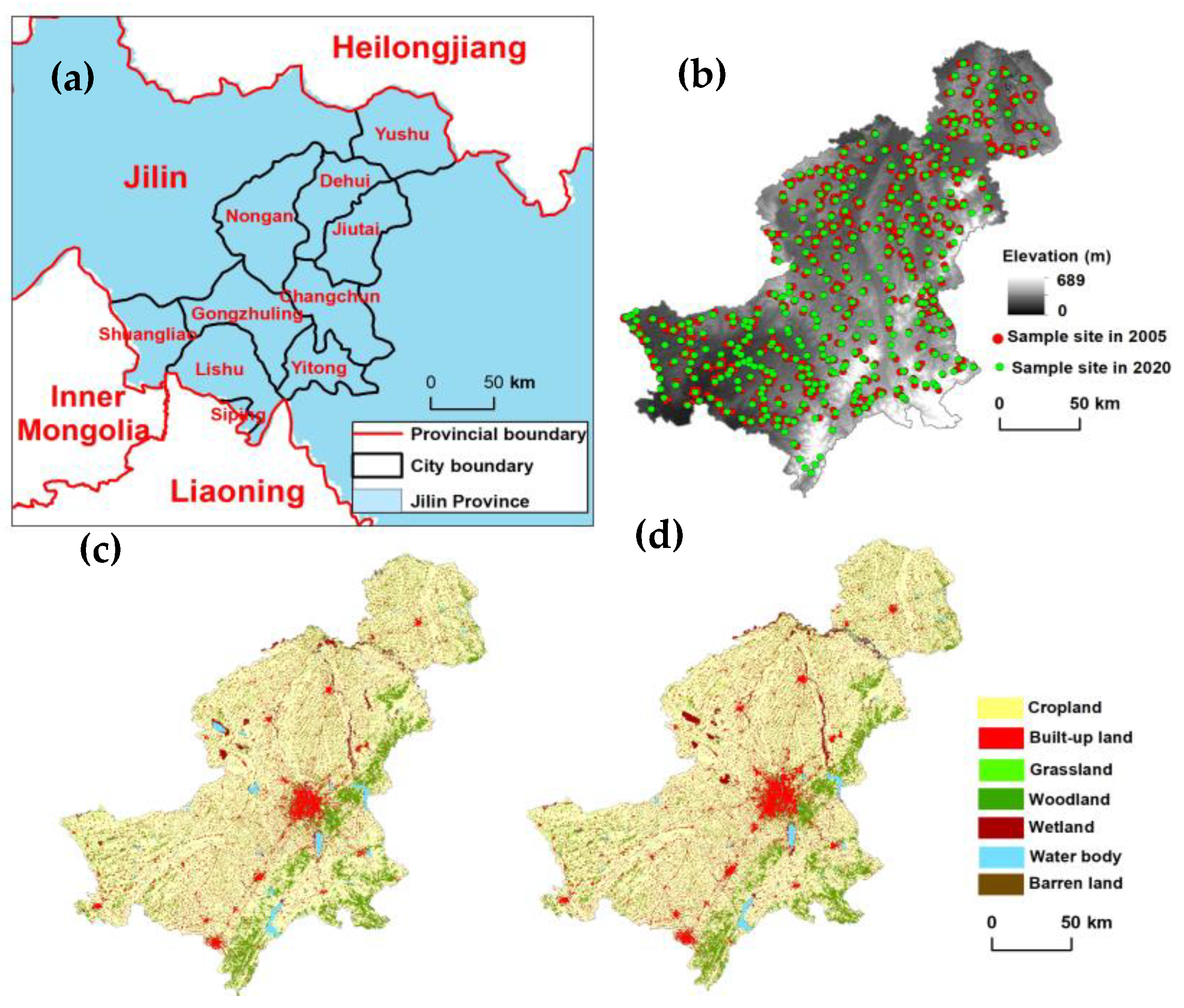
2.1. Study Area

This study was conducted in the black soil region of Jilin Province, Northeast China (Figure 1a). Extending across 42°48′ to 45°16′N latitude and 123°17′ to 127°06′E longitude, the area spans 29.1 × 10³ km² and encompasses ten counties, i.e., Changchun, Jiutai, Dehui, Nongan, Gongzhuling, Yushu, Yitong, Lishu, Shuangliao, and Siping (Figure 1a). The elevation of the study area ranges from 0 to 689 m (Figure 1b), and the slope gradient for most parts is between 1° and 5°. This region has a semi-humid continental monsoon climate in the northern temperate zone, which is characterized by four distinct seasons with cold and long winters. The annual average temperature in the region is 4.8 °C, and the annual precipitation is 582 mm with more than 70% of precipitation occurring between June and August. The zonal soil type is classified as brown forest soil (Haplic Luvisol, FAO), black soil, chernozem, and chestnut soil (Haplic Kastanozem, FAO) from east to west. Azonal soils include meadow soil, aeolian sandy soil (Haplic Arenosols, FAO), and solonetz (Haplic Solonetz, FAO) mainly. Black soil, chernozem, and meadow soil constitute 76.8% of cropland in the study area.

Anthropogenic landscapes are widely distributed in this area, and the sum of cropland and built-up land constitutes more than 80% of the total land area (Figure 1c,d). The study region has experienced unprecedented rapid urbanization in recent years, particularly after the Revitalization of Northeast China in 2003 [26]. Rapid urbanization has significantly affected landscape, air, water, biodiversity, and cropland SOC storage.

2.2. Data Source

2.2.1. Soil Sampling and Laboratory Analysis

Topsoil data at 0–20 cm depth for 569 cropland sampling sites in the study region during 2003 to 2005 were obtained from the Soil and Fertilizer Station of Jilin Province, China (Figure 1b). The data acquired included sampling location, SOC content, bulk density, and related environmental conditions. Based on the representative distribution of croplands and considering different soil types and locations of sampling points in the first period, topsoil sampling from 362 sites was performed in October 2020 (Figure 1b). Owing to prominent land cover changes, particularly the conversion from cropland to built–up land over the period 2005–2020, the scope and location of the sampling points in 2005 and 2020 differed slightly. The geographical coordinates and cropland conditions of each sampling site were recorded using a handheld global positioning system (GPS).

All soil samples were air dried and sieved though a 2–mm mesh to determine their SOC content using the potassium dichromate oxidation method via external heating in the laboratory of Northeast Institute of Geography and Agroecology, Chinese Academy of Sciences (IGA, CAS). In addition, we used ring knives with a volume of 100 cm³ (50.46 × 50 mm) to obtain the same soil samples; subsequently, we dried soil samples at a constant temperature of 105 °C and calculated soil bulk density.

2.2.2. Multitemporal Image Data

For this study, all available Landsat images from 2003 to 2005 (Landsat TM imagery) and 2018–2020 (Landsat OLI imagery) were used to synthesize bare soil images. To reduce the amount of image calculation, images obtained from April, May, October, and November, which featured no vegetation or low vegetation, were selected for synthesis. Considering cloud cover and image quality, 20 and 25 images were obtained during the above-mentioned two periods, respectively. The preprocessing steps of image synthesis were applied to a single image to establish a qualified image database that could be used for temporal mosaicking. All preprocessing was implemented using the Google Earth Engine (GEE) platform.

In addition, images captured during the sampling periods in 2005 and 2020 were used to replace the corresponding bands of bare soil synthetic images for prediction, and the results were used to assess the robustness of the composite image prediction model.

2.2.3. Land Cover Mapping

Landsat images of growing season from July to September are used for extracting land cover information. Land cover data for 2005, as interpreted from Landsat TM image, was derived from the IGA, CAS (Figure 1c). An object-based image classification approach combined with decision tree algorithm based on eCognition software was used to classify images [27], and land cover type was classified into cropland, built-up land, grassland, woodland, wetland, water body, and barren land, based on the Land Cover Classification System of China [28]. Taking the land cover data in 2005 as basic data, changes in land cover were interpreted by human-computer interaction using Landsat OLI images in 2020 (Figure 1d). Ground truth datasets, including high–resolution Google Earth images, locations obtained from the global positioning system, and landscape records of 1000 sampling points for each year, were used to assess the classification accuracy (

Table 1. Classification accuracy evaluation table.

2005	Cropland	Built-Up Land	Grassland	Woodland	Wetland	Water Body	Barren Land
CA	0.936	0.933	0.856	0.895	0.882	0.978	0.919
PA	0.950	0.936	0.910	0.901	0.835	0.899	0.832
OA	0.912
2020
CA	0.923	0.920	0.840	0.913	0.905	0.971	0.870
PA	0.957	0.945	0.850	0.921	0.874	0.859	0.798
OA	0.905

CA is consumer accuracy, PA is producer accuracy, and OA is overall accuracy.

). The overall accuracy was 0.912, and 0.905 for 2005 and 2020, respectively. Producer accuracy for cropland were 0.936, and 0.923 in 2005 and 2020, respectively.

2.2.4. Geographic Auxiliary Data

Climatic variables included mean annual precipitation (MAP), mean annual temperature (MAT), and land surface temperature (LST). Monthly precipitation and temperature data at a resolution of 1 km were downloaded from website of the National Earth System Science Data Center (NESSDC, http://www.geodata.cn (accessed on 5 October 2022)). These data were generated using more than 2400 national–level surface meteorological observation stations in China as well as digital elevation model (DEM) data as covariates; additionally, the thin-plate spline interpolation method (ANUSPLIN v4.4) was used to generate monthly precipitation data with a resolution of 1 km in China. The monthly data in the study area were extracted, and MAP and MAT were calculated. We calculated MAP and MAT for one year (2005 and 2020), five years (2001–2005 and 2016–2020), and ten years (1996–2005 and 2011–2020), which were common time intervals used for climate variables in existing literature, and compared their correlations with SOC density. MAP and MAT over five years were used to predict SOC density owing to higher correlation. Based on MOD11A2.006 Terra LST and emissivity 8–Day data with 1 km resolution, the average value of LST data in growing season (from May to September) in 2005 and 2020 was calculated and clipped via the GEE platform.

A DEM with a cell size of 30 m obtained from the NESSDC (Figure 1b) was generated by embedding and clipping based on data from NASA ASTER. These data originated from ASTER Global Digital Elevation Model V003, which was generated using stereo images collected by the ASTER instrument on Terra. Slope gradient, aspect, curvature, and topographic wetness index (TWI) were derived using DEM.

Vegetation indicators included normalized difference vegetation index (NDVI), leaf area index (LAI), and net primary productivity (NPP). Because vegetation biomass in Northeast China reached its maximum in August, LAI data products with a spatial resolution of 500 m (MOD15A2H) and NDVI data with a spatial resolution of 1 km (MOD13A2) in August were downloaded from NESSDC and clipped as indicators for forecasting SOC density. Monthly NPP data with a spatial resolution of 500 m (MOD17A3) were synthetized and clipped via the GEE platform to obtain annual NPP for the study area over the two years.

Taking into account both data volume and accuracy comprehensively, all data were resampled to a spatial resolution of 100 m as modeling factors.

3. Methodology

The flowchart of the study is descripted in Figure 2, and in this section we followed the same order. We descript (A) calculation of SOC (Section 3.1); (B) synthesis of bare soil image via temporal mosaicking (Section 3.2); (C) random forest model (Section 3.3); (D) model validation (Section 3.4); (E) comparative Model (Section 3.5); (F) importance of variables (Section 3.6).

3.1. Calculation of SOC

SOC density of the samples was calculated as follows [29].

$$SOCD=(SOC\times BD\times DEP\times (1-CF\left)\right)/10$$

(1)

where SOCD is SOC density (kg/m²), SOC is the SOC content of soil sample (g/kg), BD is bulk density (g/cm³), DEP is the thickness of the top horizon (cm), and CF is the coarse fragment fraction.

SOC storage of a specific soil unit (S_i, t) is calculated based on SOC density and unit area (A_i, km²) as follows:

$${\mathrm{S}}_{\mathrm{i}}={\mathrm{S}\mathrm{O}\mathrm{C}\mathrm{D}}_{\mathrm{i}}\times {\mathrm{A}}_{\mathrm{i}}/1000$$

(2)

3.2. Synthesis of Bare Soil Image via Temporal Mosaicking

Multitemporal mosaicking can be performed via two processes of different approaches: the image–per-pixel approach and per–data approach.

The per–pixel approach was performed based on each pixel vector of the values across time series, which was realized using a threshold mask. First, based on existing research results, four indices, i.e., the NDVI, the differences between red and green band (VG1), the differences between the near infrared band and red band (VG2), and the bare soil index (BSI), were selected to extract bare soil pixels from each image period [16]. These indices are expressed as follows.

$$\mathrm{N}\mathrm{D}\mathrm{V}\mathrm{I}=\frac{{\mathsf{\rho }}_{\mathrm{N}\mathrm{I}\mathrm{R}}-{\mathsf{\rho }}_{\mathrm{R}\mathrm{e}\mathrm{d}}}{{\mathsf{\rho }}_{\mathrm{N}\mathrm{I}\mathrm{R}}+{\mathsf{\rho }}_{\mathrm{R}\mathrm{e}\mathrm{d}}}$$

(3)

$$\mathrm{V}\mathrm{A}1={\mathsf{\rho }}_{\mathrm{R}\mathrm{e}\mathrm{d}}-{\mathsf{\rho }}_{\mathrm{B}\mathrm{l}\mathrm{u}\mathrm{e}}$$

(4)

$$\mathrm{V}\mathrm{A}2={\mathsf{\rho }}_{\mathrm{N}\mathrm{I}\mathrm{R}}-{\mathsf{\rho }}_{\mathrm{R}\mathrm{e}\mathrm{d}}$$

(5)

$$\mathrm{B}\mathrm{S}\mathrm{I}=\frac{{(\mathsf{\rho }}_{\mathrm{s}\mathrm{w}\mathrm{i}\mathrm{r}2}+{\mathsf{\rho }}_{\mathrm{R}\mathrm{e}\mathrm{d}})-({\mathsf{\rho }}_{\mathrm{N}\mathrm{I}\mathrm{R}}+{\mathsf{\rho }}_{\mathrm{B}\mathrm{l}\mathrm{u}\mathrm{e}})}{{(\mathsf{\rho }}_{\mathrm{s}\mathrm{w}\mathrm{i}\mathrm{r}2}+{\mathsf{\rho }}_{\mathrm{R}\mathrm{e}\mathrm{d}})+({\mathsf{\rho }}_{\mathrm{N}\mathrm{I}\mathrm{R}}+{\mathsf{\rho }}_{\mathrm{B}\mathrm{l}\mathrm{u}\mathrm{e}})}$$

(6)

where $\mathsf{\rho }$ is the surface reflectance (%) of the near-infrared (NIR) (for Landsat TM, NIR = B4; for Landsat OLI, NIR = B5), red (for Landsat TM, red = B3; for Landsat OLI, red = B4), blue (for Landsat TM, blue = B2; for Landsat OLI, blue = B3), and the far shortwave infrared (swir2) (for Landsat TM, swir2 = B7; for Landsat OLI, swir2 = B7).

Then, based on soil hyperspectral characteristics of the study region [30], the threshold value of each index for bare soil was determined: 0.1 < NDVI < 0.25, VG1 > 0, VG2 > 0, and BSI > 0.05.

Finally, a threshold mask was used to extract bare–soil composite images. In this process, the pixels with NDVI value less than 0.1 and exceeding 0.25, VG1 less than 0, VG2 less than 0, and BSI value less than 0.05, were denoted as ND. Pixels at coordinate (x, y) of the data that satisfied the requirements of the four indicators simultaneously were extracted as bare soil pixel and then stored in the composite image.

The per–data approach relied on a global indicator for every datum. A multi–temporal synthetic bare soil images were obtained by averaging the values of the extracted pixels that satisfied the conditions of time series.

We calculated the proportion of the extracted pixels in total cropland pixels in the study region, which exceeded 94%.

3.3. Random Forest Model

RF regression is a machine learning algorithm based on a regression tree. The model segregates data into different homogenous groups, i.e., regression trees, using recursive partitioning. Owing to the randomness introduced into the model, it has high accuracy and effective operations on large datasets. RF regression has been widely applied in SOC prediction [9].

In this method, three basic parameters require optimizations, which can optimize the RF algorithm to obtain better results. Mtry denotes the number of variables used for the binary tree in a specified node. The default value of mtry is typically one-third the number of variables in the prediction model [31]. Generally, the trial–and–error approach is adopted to obtain a relatively ideal SOC. Ntree is the number of decision trees included in the specified RF model, which can predict the SOC value via a graph when the error of the model is stable. The default value of ntree is always set at 500. The third parameter is nodesize, which is the smallest size among the terminal nodes of the regression trees. To obtain the best parameters for the RF model to predict SOC, we attempted to determine the value of mtry from 2 to 6 with an interval of 1, whereas we set the ntree values from 100 to 500 with an interval of 100. The results showed that better predictive results were obtained when mtry was selected as 4 in 2005 and 6 in 2020, ntree as 500 for both years, and the nodesize as the default value throughout the analysis.

3.4. Model Validation

The predicted results were evaluated by the coefficient of determination (R²), and root mean square error (RMSE) using stratified 10 fold cross–validation method. This validation method segregates the data into 10 randomly partitioned subsamples based on approximately equal class distributions. Nine subsamples were used as the training model, and the remaining sub–samples were used for validation. This process was repeated 10 times using different partition for validation, and the average validation was calculated as the final precision of the model [31]. The formula of RMSE is defined as the following [32]:

$$RMSE=\sqrt{\frac{{\sum }_{i=1}^n{({SOC}_{obs,i}-{SOC}_{pre,i})}^2}{n}}$$

(7)

where RMSE is the root mean square error, ${SOC}_{obs,i}$ is the observed SOC at location i, ${SOM}_{pre,i}$ is the predicted SOC at location i, and n is the total number of samples.

In addition, concordance correlation coefficient (CCC) [33] was introduced to verify the consistency between observed and predicted SOC. CCC combines the characteristics of mean square error and Pearson correlation coefficient, providing an indicator that can measure both correlation and absolute interpolation simultaneously. The CCC ${\rho }_c$ contains a measurement of precision $\rho$, and accuracy $C_b$ formula is defined as follows [33]:

$${\rho }_c=\rho C_b$$

(8)

$$C_{\mathit{b}}=\frac{2{\sigma }_{obs}{\sigma }_{pred}}{{\sigma }_{obs}^2{+\sigma }_{pred}^2+{({\mu }_{obs}-{\mu }_{pred})}^2}$$

(9)

in which, ${\rho }_c$ is CCC, $\rho$ is the correlation coefficient between the observed and predicted SOC, which measures how far each observation deviates from the best–fit line and is a measure of precision, $C_{\mathit{b}}$ is a bias correction factor that measures how far the best-fit line deviates from the 45° line through the origin and is a measure of accuracy, ${\sigma }_{obs} \mathrm{and} {\sigma }_{pred}$ are the corresponding variances; ${\mu }_{obs}$ and ${\mu }_{pred}$ are the means of the observed and predicted SOC.

The CCC can be interpreted as follows: 0–0.2 indicates poor agreement, 0.3–0.4 indicates fair agreement, 0.5–0.6 indicates moderate agreement, 0.7–0.8 indicates strong agreement, and 0.8 indicates almost perfect agreement [32].

3.5. Comparative Models

In order to verify the reliability of the methods used in this study, we chose comparative models for accuracy comparison. We attempted to replace the corresponding band of the bare soil composite image in predictive model with that of the single image in 2005 and 2020, respectively, to verify the superiority of introducing bare soil variables into the RF model. Multiple linear regression (MLR) and support vector machine (SVM) were employed to test the advantages of the RF model in predicting soil organic carbon.

MLR is a popular algorithm that can identify linear relationships between SOC and environmental variables. However, the algorithm cannot identify non–linear relationships. In order to eliminate the feature of multicollinearity between variables, we selected variables with a VIF less than 10 for prediction. In 2005 and 2020, 11 and 12 variables were retained to participate in the model’s predictions, respectively.

The concept of the SVM model is derived from the principles of statistical learning theory, and then applied to classification and regression tasks through the process of structural risk minimization [32]. The advantages of SVM model are to handle small samples, as well as non–linear and high–dimensional data. The SVM algorithm was executed in e1071 package of R language. The kernel is set to the radial basis function kernel.

3.6. Importance of Variables

The importance of variables used in the RF model in RStudio was calculated based on the “IncMSE”, i.e., the percentage increase in the mean square error. The indicator values were measured by assigning randomly values to each predictive variable. If the predicted variable is more important, then the error in the prediction model increases after its value is replaced randomly. The greater value of IncMSE signifies the greater importance of the variable [16].

4. Results

4.1. Accuracy Evaluation of Bare Soil Images and Prediction Results

Overall, comprehensive judgment of four indicators significantly achieved a good result in bare soil extraction (Figure 3).

The extraction ratios of bare soil pixels during the two study periods reached 96.6% and 94. 2%, respectively. In 2003–2005, bare soil extraction frequency between 5–7 and 7–10 times accounted for 12.2% and 69.5%, respectively. In 2018–2020, bare soil extraction frequency between 3–5, 5–7, and 7–10 times accounted for 10.3%, 15.6%, and 53.6%, respectively (Figure 3a,b). Figure 3c–j showed monthly frequency of bare soil in April, May, October and November calculated over three years of two periods. From 2003 to 2005, the extracted bare soil area in April was the smallest and the proportion of frequencies below 3 reached 65%. In May, the extracted area was second only to November, and the proportion of frequencies above 3 was 80.3% (Figure 3c–f). From 2018 to 2020, the image quality in April and May was significantly higher than that in October and November. The extracted area in April was slightly higher than that in May, but the proportion of bare soil frequencies below 3 reached 44.9%. In May, the area with bare soil frequencies above 3 was smaller than the former period, but it still reached 66.81% (Figure 3g–j).

CCC in 2005 was 0.755, and 0.580 in 2020, indicating a strong agreement in 2005, and moderate agreement in 2020, respectively. R² for linear regression of observed SOMD and predicted SOMD was 0.677, and 0.644 in 2005 and 2020, respectively (Figure 4).

Comparative experiments with RF__single, MLR and SVM were performed to prove the superiority of the method (

Table 2. Accuracy comparison of different models.

	RF_bare		RF_single		MLR		SVM
	2005	2020	2005	2020	2005	2020	2005	2020
R2	0.58	0.53	0.51	0.43	0.34	0.45	0.38	0.23
RMSE (kg/m2)	0.82	0.84	0.84	0.86	0.97	0.85	0.98	1.01

). The coefficient of determination of RF__bare was 0.58 and 0.53 in 2005 and 2020, with RMSE of 0.82 and 0.84, respectively. Overall, the prediction accuracy of RF is relatively high, except for the MLR model in 2020 which has a higher accuracy than R_{_single}. RF__bare has a high coefficient of determination and a low RMSE, which advantaged than R__single. The accuracy of each model in 2020 was lower than that in 2005 except for MLR.

In addition, due to significant differences in data accuracy in the study, we conducted a comparative analysis of the impact of climate data with a spatial resolution of 1 km on the prediction results. We extracted 1000 grids completely within the cropland scope for the years 2005 and 2020, which captured the pixel positions of the climate data to ensure consistency between statistical grids and climate data grids, and avoided the influence of incomplete pixels at cropland edges. We calculated the mean value of SOCD (SOCD__mean) within each 1 km² grid and extracted the SOCD value (SOCD_c) for the central point of that grid. We then analyzed the correlation between the SOCD__mean and SOCD_c with MAT and MAP data for each grid (point). Results show that there is a very significant correlation between the SOCD__mean and SOCD_c (correlation coefficient was 0.985 and 0.972 in 2005 and 2020, respectively), and the correlation between the SOCD__mean and climate data is higher than that of SOCD_c (

Table 3. The impact of climate data on model results.

	SOCD_c		MAT		MAP
	2005	2020	2005	2020	2005	2020
SOCD_mean2005	0.985 **		−0.626 **		0.538 **
SOCD_c2005	1		−0.609 **		0.527 **
SOCD_mean2020		0.972 **		−0.611 **		0.605 **
SOCD_c2020		1		−0.601 **		0.589 **

** Significant correlation at 0.001 level.

).

4.2. Changes in SOC Density of Croplands

SOC of croplands within the region varies between 1.2 kg/m² and 6.7 kg/m², with an average value of 3.42 kg/m² and 3.32 kg/m² in 2005 and 2020, respectively (Figure 5a,b). In 2005, the low–value areas with an SOC density of less than 2.5 kg/m² were mainly distributed in the southwest of Shuangliao and Lishu, which constituted 10.81% of the total cropland area. The SOC density for most area varied between 3.0–3.5 and 3.5–4.0 kg/m², and constituted 24.35% and 33.53% of the total cropland area, respectively; furthermore, the areas were mainly distributed in Nongan, Lishu and Siping. The high–value areas featuring an SOC density exceeding 4.0 kg/m² were mainly distributed in the central region of the study area, and constituted 21.81% of the total cropland area. In 2020, the low-value area constituted only 5.93% of the total cropland area. Croplands with SOC density ranging from 3.0 to 3.5 kg/m² were distributed widely, and constituted 54.29% of the total cropland area. The high–value areas constituted only 3.71% of the total area, and was concentrated in the east of the study area. During the research period, 62.14% of croplands with SOC density greater than 4.0 kg/m² decreased significantly, and 38.60% of croplands with SOC density between 2.5–3.0 kg/m² have significantly increased.

From 2005 to 2020, 44.85% of croplands decreased greater than 0.5 kg/m² in SOC density, and 41.58% of croplands decreased between 0.5 and 1.5 kg/m². 12.99% of croplands showed an increase in SOC greater than 0.5 kg/m², and 10.93% of croplands varied between 0.5 and 1.5 kg/m² (Figure 5c). The croplands with significant decline were concentrated in the central and southwestern regions, whereas those with significant increase were concentrated in the east region, including most part of Jiutai, east part of Changchun and Shuangliao, and west part of Gongzhuling. 41.12% of croplands had relatively stable SOC density, with a change within 0.5 kg/m².

4.3. Changes in SOC Storage

SOC storage of topsoil for croplands in the study area decreased from 89.96 Tg C in 2005 to 82.79 Tg C in 2020, which represents a total decrease of 7.17 Tg C (7.97%) and an annual decrease of 0.48 Tg C yr⁻¹. In addition to Jiutai, Shuangliao and Lishu, the other seven counties showed decreased SOC storage. SOC storages of croplands in Changchun and Nongan decreased notablely by 2.40 Tg C and 2.04 Tg C, respectively, which constituted 62.21% of the total decrease in SOC storage. Among the counties with increasing SOC storage, the increases exhibited by Jiutai and Shuangliao were the most significant, i.e., 1.29 Tg C and 1.11 Tg C, respectively (Figure 6a).

Rapid urbanization process affected regional differences in SOC storage of croplands in the study area. In the past 15 years, cropland area occupied by built–up land was 597.37 km², which constituted 69.16% of the total area of cropland transformed out (Figure 6b). Owing to the expansion of built–up land, the area of cropland has significantly decreased, resulting in the loss of 2.20 Tg C in SOC of croplands by soil sealing, and leading to fluctuations in soil carbon input (Figure 6b). The average SOC density of cropland occupied by built–up land in 2005 was 3.74 kg/m², which was higher than the average value of total croplands in 2005.

4.4. The Relative Importance of Environmental Data

The relative importance (RI) of the predictors in the SOC density modeling was calculated based on the percentage increase in the average standard error (%IncMSE) and converted to 100% (Figure 7). Climate, with RI of 44.64% and 37.26% in 2005 and 2020, respectively, was the most important environmental factor that explained the variation in SOC density. During these two years, MAT was more important than MAP and LST, and its percentage exceeded 20% in 2005. Synthetic images of bare soil have a relatively higher RI of 23.54% and 26.29% in 2005 and 2020, respectively, and the RI of each band was different. In 2005 and 2020, B5 and B1 contributed the most, with RI of 5.34% and 7.32%, respectively. The RI of topographic variables in 2005 and 2020 was 19.50% and 21.80%, respectively, and that of the DEM was 8.61% and 8.99%, respectively. Vegetation variables indicated the lowest RI among the four factors, i.e., 12.31% and 14.65% in 2005 and 2020, respectively. In addition, except for the RIs of climate variables, the RIs of synthetic image of bare soil, topographic factors, and vegetation variables increased from 2005 to 2020.

5. Discussion

5.1. Random Forest Model Incorporating Bare Soil Images

The application of bare composite image obtained by stacking multitemporal images has been proven to be an effective method for removing the interference of high vegetation cover in landscapes when predicting soil properties at a large scale [15,34,35]. In some studies pertaining to multitemporal series image mosaics, the results revealed that the time period should be considered because any changes in soil within or across five–year periods are caused by small scale variabilities due to agricultural practices, land cover changes, soil degradation or soil erosion. Dematê et al. applied all Landsat scenes available during the period 1985–2017 to maximize bare soil area in a large agricultural region and increased the total bare soil area to 90% [34]. In this study, using soil spectral characteristics of the study area and bare soil thresholds reported in the existing literatures, we applied the combinations of BSI, NDVI, VG1, and VG2 to extract bare soil. Based on three years of images, the extracted bare soil in both periods exceeded 94% of the total cropland, owing to the environmental characteristics of Northeast China. We compared the results of SOC density predicted using monotemporal images and the multitemporal series image, and discovered that the prediction results involving composite images were higher than those of the monotemporal images in the two years (Table 2). The RI of the synthetic images of bare soil in 2005 and 2020 was 23.53% and 26.29%, respectively (Figure 7). This shows a promising prospects of multiple temporal series images for improving the prediction accuracy of soil attributes at a large scale.

However, we can see that the prediction accuracy in this study is lower than that of Geng et al. [35], but slightly higher than the result of Vaudour et al. [16]. In addition, there are large differences between the two years. This variability can be caused by differences between Landsat sensors, or differences in soil moisture and soil surface roughness caused by different weather conditions and land management in different time periods, or different sampling locations and variable timeframes (eg. samples from 2003 to 2005 in this study). All these could influence the surface reflectance of the soil (also discussed in Diek et al. [36]). The use of the mean over the three–year periods reduces variability, which makes the performance of RF__bare Model superior to that of RF__single. However, as Figure 3 shows, the bareness frequency changes for each period. The frequency extraction of bare soil in 2020 was significantly lower than that in 2005, which may be one of the reasons for the lower accuracy of SOC prediction in 2020.

In general, the prediction performance of machine learning algorithms for SOC is highly effective. Even though Castaldi et al. [37] indicated that the performance of the RF model was not optimal and that the correlation between variables was weak, the RF algorithm was still used to bond reflectance and SOC in many studies, and a predictive model with high consistency was obtained. RF performed regression tasks by multiple decision regression trees, and retrieved SOC by weighted average of regression results according to variable importance (Figure 7). Meanwhile, RF makes comprehensive and in–depth data mining analysis on independent variables both in regression and classification [38]. In this study, RF had more advantages than MLR, and SAV in this study except MLR model in 2020.

Although there have been some studies employing machine learning methods to predict soil properties with small samples (45 soil samples, Liu et al. [38]; 74 soil samples, Wei et al., 2021 [39]; 93 samples, Habibi et al., 2020 [40]), and the results show that machine learning methods have better predictive accuracy compared to PLSR and SVRS [38]. Studies by Zuo et al. [41] have shown that large sample sizes are more conducive to demonstrate the advantages of machine learning methods. In our study, the number of samples in 2020 was still insufficient compared to that in 2005, which had a possible negative impact on the prediction results, and resulting a lower accuracy of SOC in 2020 than in 2005.

In addition, the accuracy of climate data has an impact on prediction results (Table 3). The comparative analysis showed that although high-precision environmental factors such as DEM and vegetation reflect some of the differences in soil characteristics within 1 km, the climate data indeed causes a convergence in prediction results within the unit area. The application of higher-precision climate data will improve prediction accuracy to a certain extent.

5.2. Dynamics of SOC Stock in Topsoil of Croplands from 2005 to 2020

The average SOC density of croplands in the study region was 3.42 and 3.32 kg/m² in 2005 and 2020, respectively. These predicted values were slightly higher than the value predicted (3.28 kg/m² in 2005) by Zhang et al. using the area-weighted method of soil type based on sampling points [24], but lower than those obtained by Han et al. in the same region [25]. These differences are attributable to changes in SOC density in croplands as well as the methodologies used. By fully considering the environmental factors affecting SOC of croplands, the SOC density for croplands in 2005 and 2020 was predicted using same sampling design and analytical methods. Compared with the previous dynamic analysis benchmarked on soil survey [25], where gravel in soils and spatial discrepancies in soil depths were disregarded, the accuracy of the RF model was higher, and the results of this study were more comparable at different time.

Campo indicated that climate warming overall increased cropland carbon sink though the replacement of SOC lost by erosion increases but the preservation of deposited C decreases under warming [42]. Yu et al. showed that most croplands in China manifested a significant increase in SOC storage, whereas only a few zones (mainly in Northeast China) showed a decrease during 1980–2009 [43]. Research of Man et al. revealed that SOC storage in croplands of the Sanjiang Plain of Northeast China increased owing to the increasing cropland area, but mean value of SOC density decreased during 2000–2010 [5]. Ou et al. studied changes in SOC content of Jilin Province, and found that SOC content in the middle corn belt (almost the same region as in the present study) decreased markedly from 1980 to 2010 [44]. These studies consistently indicated that SOC in the study area decreased before 2010. Han et al. studied SOC density in topsoil of croplands all over the country from 1988 to 2019 and discovered that SOC in Northeast China decreased during 1980–2008 and then increased [25]. Mao et al. compared cropland topsoil SOC storage obtained through sampling analysis with those of profiles derived from China’s National Soil Inventory during the 1980s and indicated that topsoil SOC storage has increased significantly due to increased soil C input and the return of corn stubble into soil over the past three decades [9]. Our study showed that from 2005 to 2020, the density and storage of SOC in croplands in the study region decreased, and that the temporal and spatial differences were remarkable. These differences may be caused by different data, methods, research periods, as well as reflect the feature of topsoil SOC of croplands in the black soil region with rapid urbanization. Spatially, SOC density and storage of croplands in the middle region decreased the most, whereas those in Jiutai and Shuangliao increased significantly. This trend reveals a rapid decline in organic carbon in croplands with high initial value and an improvement in croplands with low initial values.

5.3. The Drving Factors of SOC Prediction Models

Previous studies showed that the driving factors of SOC prediction varied in different study areas and periods [43]. In general, SOC density depends highly on the climate regime: it decreases with temperature but increases with precipitation [45]. Over the past two decades, climate of the study region became milder and more humid. Different combinations of water and heat ratio can affect their effects on SOC [42]. The RIs of MAT and MAP for SOC density prediction were 20.90% and 14.93%, and 15.69% and 14.70% in 2005 and 2020, respectively (Figure 7). Temperature was the most important factor governing changes in SOC density at the regional scale, which is consistent with most results in the literature for Northeast China [46,47]. Increased surface temperature and evapotranspiration increase plant respiration rate, accelerate the decomposition of soil organic matter, thereby reducing the content of SOC [48].

Due to the heterogeneity of the environment, the impact of terrain variables varied remarkably in different region. Study of Chen showed that TWI was the first important factor for all compared models in Wuhan because the terrain factor can quantitatively describe the balance between water accumulation and drainage conditions [49]. However, consistent with more existing studies [50], our study showed that elevation played the most important role among terrain variables in the SOC prediction. The importance of elevation in SOC density may originated from its correlation with temperature, parent material, soil type, water, and land cover etc., which can’t be revealed by coarser information of climate.

LST is a variable representing soil water and heat status, which exhibited RI of 6.88% and 5.61% in the two years, thus indicating the effect of LST on the distribution of SOC density in croplands and its prospect of improving the projection accuracy of SOC. Among vegetation factors, the RI of NPP to SOC was higher in both years, thereby indicating a strong correlation between NPP and soil SOC density [51].

Urbanization not only limits the input of soil carbon in cropland, but also leads to the loss of surface organic carbon due to soil sealing caused by land use changes. Because the study area is also located at the core of Harbin–Changchun Urban Agglomeration, the impact of urbanization as an extreme human activity on SOC of cropland cannot be ignored. Owing to the expansion of built–up land, the total loss of topsoil organic carbon of croplands in study area was 2.20 Tg C from 2000 to 2020 (Figure 6). The average SOC density of cropland occupied by built–up land in 2005 was 3.74 kg/m², higher than the average SOC density of croplands in the study region in 2005 (3.42 kg/m²) (Figure 5), which indicated that urban expansion occupied high–quality croplands, and cropland protection needs to be included in reasonable urban planning.

6. Conclusions

In this study, four indices were jointed to extract bare soil pixel, and the per–pixel and per–data approach were used to build bare soil composite images during 2003–2005, and 2018–2020, which improved the area of bare soil extraction. The random forest model that integrates bare soil composite images improve the accuracy and robustness of SOC density prediction. During 2005–2020, total organic carbon storage of topsoil in the Black Soil Region of Jilin Province, China decreased from 89.96 to 82.79 Tg C, and SOC density decreased from 3.42 kg/m² to 3.32 kg/m². Changes of SOC represented significant heterogeneity spatially. 62.14% of cropland with SOC density greater than 4.0 kg/m² decreased significantly, and 38.60% of cropland with SOC density between 2.5–3.0 kg/m² have significantly increased. SOC density in Jiutai and the southern region of Shuangliao increased, whereas those in the western region of Changchun and the southeastern region of Nongan decreased remarkably. Climatic factors made great contributions to SOC density, however, their relative importance decreased during study period. The occupation of cropland caused by urban expansion has resulted in a significant loss of organic carbon in croplands. On one hand, it is necessary to increase soil C input to address global climate change; on the other hand, for the black soil areas with rapid urbanization, it is necessary to coordinate cropland protection and urban development.

References

1. Jiang, G.Y.; Xu, M.G.; He, X.H.; Zhang, W.J.; Huang, S.M.; Yang, X.Y.; Liu, H.; Peng, C.; Shirato, Y.; Lizumi, T.; et al. Soil organic carbon sequestration in upland soils of northern China under variable fertilizer management and climate change scenarios. Glob. Biogeochem. Cycles 2014, 28, 319–333. [Google Scholar] [CrossRef]
2. Luo, Z.K.; Wang, G.C.; Wang, E.L. Global subsoil organic carbon turnover times dominantly controlled by soil properties rather than climate. Nat. Commun. 2019, 10, 3688. [Google Scholar] [CrossRef]
3. Xie, E.Z.; Zhang, X.; Lu, F.Y.; Peng, Y.X.; Zhao, Y.C. Spatiotemporal changes in cropland soil organic carbon in a rapidly urbanizing area of southeastern China from 1980 to 2015. Land Degrad. Dev. 2022, 33, 1323–1336. [Google Scholar] [CrossRef]
4. Gál, A.; Vyn, T.J.; Michéli, E.; Kladivko, E.J.; McFee, W.W. Soil carbon and nitrogen accumulation with long-term no-till versus moldboard plowing overestimated with tilled-zone sampling depths. Soil Tillage Res. 2007, 96, 42–51. [Google Scholar] [CrossRef]
5. Man, W.D.; Yu, H.; Li, L.; Liu, M.Y.; Mao, D.H.; Ren, C.Y.; Wang, Z.M.; Jia, M.M.; Miao, Z.H.; Lu, C.Y.; et al. Spatial expansion and soil organic carbon storage changes of croplands in the Sanjiang Plain, China. Sustainability 2017, 9, 563. [Google Scholar] [CrossRef]
6. Yu, Y.Q.; Huang, Y.; Zhang, W. Projected changes in soil organic carbon stocks of China’s croplands under different agricultural managements, 2011–2050. Agric. Ecosyst. Environ. 2013, 178, 109–120. [Google Scholar] [CrossRef]
7. Yang, R.M.; Zhang, G.L.; Liu, F.; Lu, Y.Y.; Yang, F.; Yang, F.; Yang, M.; Zhao, Y.G.; Li, D.C. Comparison of boosted regression tree and random forest models for mapping topsoil organic carbon concentration in an alpine ecosystem. Ecol. Indic. 2016, 60, 870–878. [Google Scholar] [CrossRef]
8. Zhao, M.S.; Rossiter, D.G.; Li, D.C.; Zhao, Y.G.; Liu, F.; Zhang, G.L. Mapping soil organic matter in low-relief areas based on land surface diurnal temperature difference and a vegetation index. Ecol. Indic. 2014, 39, 120–133. [Google Scholar] [CrossRef]
9. Odebiri, O.; Mutanga, O.; Odindi, J.; Peerbhay, K.; Dovey, S. Predicting soil organic carbon stocks under commercial forest plantations in KwaZulu-Natal province, South Africa using remotely sensed data. GISci. Remote Sens. 2020, 57, 450–463. [Google Scholar] [CrossRef]
10. Li, X.Y.; Shang, B.B.; Wang, D.Y.; Wang, Z.M.; Wen, X.; Kang, Y.D. Mapping of soil organic carbon and total nitrogen of croplands in the Corn Belt of Northeast China based on a geographically weighted regression Kriging model. Comput. Geosci. 2020, 135, 104392. [Google Scholar] [CrossRef]
11. Martin, M.P.; Orton, T.G.; Lacarce, E.; Meersmans, J.; Saby, N.P.A.; Paroissien, J.B.; Jolivet, C.; Boulonne, L.; Arrouays, D. Evaluation of modelling approaches for predicting the spatial distribution of soil organic carbon stocks at the national scale. Geoderma 2014, 223, 97–107. [Google Scholar] [CrossRef]
12. Mao, D.H.; Wang, Z.M.; Li, L.; Miao, Z.H.; Ma, W.H.; Song, C.C.; Ren, C.Y.; Jia, M.M. Soil organic carbon in the Sanjiang Plain of China: Storage, distribution and controlling factors. Biogeosciences 2015, 12, 1635–1645. [Google Scholar] [CrossRef]
13. Wang, B.; Waters, C.; Orgill, S.; Gray, J.; Cowie, A.; Clark, A.; Liu, D.L. High resolution mapping of soil organic carbon stocks using remote sensing variables in the semi-arid rangelands of eastern Australia. Sci. Total Environ. 2018, 630, 367–378. [Google Scholar] [CrossRef]
14. Wang, K.; Qi, Y.B.; Guo, W.J.; Zhang, J.L.; Chang, Q.R. Retrieval and mapping of soil organic carbon using Sentinel-2A spectral images from bare cropland in Autumn. Remote Sens. 2021, 13, 1072. [Google Scholar] [CrossRef]
15. Rogge, D.; Bauer, A.; Zeidler, J.; Mueller, A.; Esch, T.; Heiden, U. Building an exposed soil composite processor (SCMap) for mapping spatial and temporal characteristics of soils with Landsat Imagery (1984–2014). Remote Sens. Environ. 2018, 205, 1–17. [Google Scholar] [CrossRef]
16. Vaudour, E.; Gomez, C.; Lagacherie, P.; Loiseau, T.; Baghdadi, N.; Urbina-Salazar, D.; Loubet, B.; Arrouays, D. Temporal mosaicking approaches of Sentinel-2 images for extending topsoil organic carbon content mapping in croplands. Int. J. Appl. Earth Obs. 2021, 96, 102277. [Google Scholar] [CrossRef]
17. Nascimento, C.M.; Mendes, W.d.S.; Silvero, N.E.Q.; Poppiel, R.R.; Sayão, V.M.; Dotto, A.C.; Santos, N.V.d.; Amorim, M.T.A.; Demattê, J.A.M. Soil degradation index developed by multitemporal remote sensing images, climate variables, terrain and soil atributes. J. Environ. Manag. 2021, 277, 111316. [Google Scholar] [CrossRef] [PubMed]
18. Mzid, N.; Pignatti, S.; Huang, W.J.; Casa, R. An analysis of bare soil occurrence in Arable croplands for remote sensing topsoil applications. Remote Sens. 2021, 13, 474. [Google Scholar] [CrossRef]
19. Zhao, Y.M.; Chen, L.P.; Li, J.J.; Chu, C.J.; Huang, F.; Che, J.B.; Zhang, C.; Li, C.C. Research on the definition of soil types in typical black soil regions of Northeast China. Sci. Soil Water Conserv. 2020, 4, 123–129. [Google Scholar]
20. Yan, B.X.; Yang, Y.H.; Liu, X.T. Current situation and evolutive trend of soil erosion in black soil region of northeast China. Chin. J. Soil Water Conserv. 2008, 12, 26–30. (In Chinese) [Google Scholar]
21. Wang, L.X.; Cai, Q.G.; Shen, B. Soil and water conservation and soil improvement in the black soil region of northeast China. In Research on Several Strategic Issues Concerning the Allocation of Soil and Water Resources, Ecological and Environmental Protection, and Sustainable Development in the Northeast Region (Agriculture Volume); Shi, Y., Ed.; Science Press: Beijing, China, 2007; pp. 230–231. [Google Scholar]
22. Liu, B.Y.; Yan, B.X.; Shen, B. Current status of agricultural land soil erosion and comprehensive management strategies in the black soil region of Northeast China. Chin. J. Soil Water Conserv. 2008, 6, 1–8. [Google Scholar]
23. Gong, Z.T. Soil Genesis and Systematic Classification; Science Press: Beijing, China, 2007. [Google Scholar]
24. Zhang, C.H.; Wang, Z.M.; Ren, C.Y.; Song, K.S.; Zhang, B.; Liu, D.W. Spatial and temporal changes of organic carbon in agricultural soils of Songnen Plain Maize belt. Trans. CSAE 2010, 26, 300–307. (In Chinese) [Google Scholar]
25. Han, T.F.; Du, J.X.; Qu, X.L.; Ma, C.B.; Wang, H.Y.; Huang, J.; Liu, K.L. Factors affecting change in topsoil organic carbon pool density in Chinese farmlands from 1988 to 2019. J. Plant Nutr. Fertil. 2022, 28, 1145–1157. (In Chinese) [Google Scholar]
26. Li, X.Y.; Yang, L.M.; Ren, Y.X.; Li, H.Y.; Wang, Z.M. Impacts of urban sprawl on soil resources in the Changchun–Jilin Economic Zone, China, 2000–2015. Int. J. Environ. Res. Public Health 2018, 15, 1186. [Google Scholar] [CrossRef] [PubMed]
27. Mao, D.H.; Tian, Y.L.; Wang, Z.M.; Jia, M.M.; Du, J.; Song, C.C. Wetland changes in the Amur River Basin: Differing trends and proximate causes on the Chinese and Russian sides. J. Environ. Manag. 2021, 1, 111670. [Google Scholar] [CrossRef] [PubMed]
28. Wu, B.F. Land cover in China; Science Press: Beijing, China, 2017. (In Chinese) [Google Scholar]
29. Mann, L.K. Changes in soil carbon storage after cultivation. Soil Sci. 1986, 142, 279–288. [Google Scholar] [CrossRef]
30. Li, X.Y.; Shi, Z.Y.; Xing, Z.H.; Wang, M.; Wang, M.C. Dynamic evaluation of cropland degradation risk by combining multi-temporal remote sensing and geographical data in the Black Soil Region of Jilin Province, China. Appl. Geogr. 2023, 154, 102920. [Google Scholar] [CrossRef]
31. Bangelesa, F.; Adam, E.; Knight, J.; Dhau, I.; Ramudzuli, M.; Mokotjomela, T.M. Predicting soil organic carbon content using hyperspectral remote sensing in a degraded mountain landscape in Lesotho. Appl. Environ. Soil Sci. 2020, 2020, 1–11. [Google Scholar] [CrossRef]
32. Usowicz, B.; Marczewski, W.; Usowicz, J.B.; Lukowski, M.; Lipiec, J. Comparison of surface soil moisture from SMOS satellite and ground measurement. Int. Agrophys. 2014, 28, 359–369. [Google Scholar] [CrossRef]
33. Lin, L.I.-K. A concordance correlation coefficient to evaluate reproducibility. Biometrics 1989, 45, 255–268. [Google Scholar] [CrossRef]
34. Demattê, J.A.M.; Huete, A.R.; Ferreira, L.G.; Nanni, M.R.; Alves, M.C.; Fiorio, P.R. Methodology for bare soil detection and discrimination by Landsat TM Image. Open Remote Sens. J. 2009, 2, 24–35. [Google Scholar] [CrossRef]
35. Geng, J.; Tan, Q.; Lv, J.; Fang, H. Assessing spatial variations in soil organic carbon and C: N ratio in Northeast China’s black soil region: Insights from Landsat-9 satellite and crop growth information. Soil Till. Res. 2024, 1, 105897. [Google Scholar] [CrossRef]
36. Diek, S.; Fornzllaz, F.; Schaepman, M.E.; Jong, R.D. Barest pixel composite for agricultural areas using Landsat time series. Remote Sens. 2017, 9, 1245. [Google Scholar] [CrossRef]
37. Castaldi, F.; Palombo, A.; Santini, F.; Pascucci, S.; Pignatti, S.; Casa, R. Evaluation of the potential of the current and forthcoming multispectral and hyperspectral imagers to estimate soil texture and organic carbon. Remote Sens. Environ. 2016, 179, 54–65. [Google Scholar] [CrossRef]
38. Liu, Q.; He, L.; Guo, L.; Wang, M.D.; Deng, D.P.; LV, P.; Wang, R.; Jia, Z.F.; Hu, Z.W.; Wu, G.F.; et al. Digital mapping of soil organic carbon density using newly developed bare soil spectral indices and deep neural network. Catena 2022, 219, 106603. [Google Scholar] [CrossRef]
39. Wei, L.; Zhang, Y.; Lu, Q.; Yuan, Z.; Li, H.; Huang, Q. Estimating the spatial distribution of soil total arsenic in the suspected contaminated area using uav-borne hyperspectral imagery and deep learning. Ecol. Ind. 2021, 133, 108384. [Google Scholar] [CrossRef]
40. Habibi, V.; Ahmadi, H.; Jafari, M.; Moeini, A. Machine learning and multispectral data-based detection of soil salinity in an arid region. Central Iran. Environ. Monit. Assess. 2020, 192, 759. [Google Scholar] [CrossRef] [PubMed]
41. Zuo, W.G.; Gu, B.X.; Zou, X.W.; Peng, K.; Shan, Y.L.; Yi, S.Q.; Shan, Y.H.; Gu, C.H.; Bai, Y.C. Soil organic carbon sequestration in croplands can make remarkable contributions to China’s carbon neutrality. J. Clean. Prod. 2023, 382, 135268. [Google Scholar] [CrossRef]
42. Campo, J.L. Warming to increase cropland carbon sink. Nat. Clim. Chang. 2023, 13, 121–122. [Google Scholar] [CrossRef]
43. Ou, Y.; Rousseau, A.N.; Wang, L.X.; Yan, B.X. Spatio-temporal patterns of soil organic carbon and pH in relation to environmental factors—A case study of the black soil region of Northeastern China. Agric. Ecosyst. Environ. 2017, 245, 22–31. [Google Scholar] [CrossRef]
44. Yu, Y.Q.; Huang, Y.; Zhang, W. Modelling soil organic carbon change in croplands of China, 1980–2009. Glob. Planet Chang. 2012, 82–83, 115–128. [Google Scholar] [CrossRef]
45. Li, H.; Pei, J.B.; Wang, J.K.; Li, S.Y.; Gao, G.W. Organic carbon density and storage of the major black soil regions in Northeast China. J. Soil Sci. Plant Nut. 2013, 13, 883–893. [Google Scholar] [CrossRef]
46. Liu, X.J.; Zhang, Y. Identification of key factors limiting topsoil organic carbon in China. Environ. Earth Sci. 2022, 81, 533. [Google Scholar] [CrossRef]
47. Hunt, J.R.; Celestina, C.; Kirkegaard, J.A. The realities of climate change, conservation agriculture and soil carbon sequestration. Glob. Chang. Biol. 2020, 26, 3188–3189. [Google Scholar] [CrossRef] [PubMed]
48. Ren, W.; Tian, H.Q.; Tao, B.; Huang, Y.; Pan, S.F. China’s crop productivity and soil carbon storage as influenced by multifactor global change. Glob. Chang. Biol. 2012, 18, 2945–2957. [Google Scholar] [CrossRef] [PubMed]
49. Chen, D.; Chang, N.J.; Xiao, J.F.; Zhou, Q.B.; Wu, W.B. Mapping dynamics of soil organic matter in cropland with MODIS data and machina learning algorithms. Sci. Total Environ. 2019, 669, 844–855. [Google Scholar] [CrossRef] [PubMed]
50. Rostaminia, M.; Rahmani, A.; Mousavi, S.R.; Tahizadeh-Mehrjardi, R.; Maghsodi, Z. Spatial prediction of soil organic carbon stocks in an arid rangeland using machine learning algorithms. Environ. Monit. Assess. 2021, 193, 815. [Google Scholar] [CrossRef]
51. Sun, L.Y.; Song, F.B.; Liu, S.Q.; Cao, Q.J.; Liu, F.L.; Zhu, X.C. Integrated agricultural management practice improves soil quality in Northeast China. Arch. Agron. Soil. Sci. 2018, 64, 1932–1943. [Google Scholar] [CrossRef]
Figure 1. Location of the study region (a), elevation and sampling sites (b), land cover in 2005 (c) and 2020 (d).
Remotesensing 16 02010 g001
Figure 2. Flowchart of the study.
Remotesensing 16 02010 g002
Figure 3. Map of the frequency of bare soil detection during 2003–2005 (a), and 2018–2020 (b), monthly frequency in April, May, October, and November during 2003–2005 (cf), and 2018–2020 (gj) (0.1 < ND, VI < 0.25, VG1 > 0, VG2 > 0, and BSI > 0.05).
Remotesensing 16 02010 g003
Figure 4. Accuracy evaluation of RF_bare in 2005 (a), and 2020 (b).
Remotesensing 16 02010 g004
Figure 5. Distribution of SOCD in 2005 (a) and 2020 (b) and difference (c).
Remotesensing 16 02010 g005
Figure 6. Topsoil SOC storage for croplands in counties (a), SOC storage loss caused by conversion from cropland into built–up land and its proportion to total SOC storage of transferred cropland (b).
Remotesensing 16 02010 g006
Figure 7. RI of covariates for predicting SOC density using RF model in 2005 (a) and 2020 (b), which are shown in the decreasing order and converted to 100%.
Remotesensing 16 02010 g007