Abstract
Limited resources for edge computing platforms in airborne and spaceborne imaging payloads prevent using complex image processing models. Model pruning can eliminate redundant parameters and reduce the computational load, enhancing processing efficiency on edge computing platforms. Current challenges in model pruning for remote-sensing object detection include the risk of losing target features, particularly during sparse training and pruning, and difficulties in maintaining channel correspondence for residual structures, often resulting in retaining redundant features that compromise the balance between model size and accuracy. To address these challenges, we propose the L1 reweighted regularization (L1RR) pruning method. Leveraging dynamic and self-adaptive sparse modules, we optimize L1 sparsity regularization, preserving the model’s target feature information using a feature attention loss mechanism to determine appropriate pruning ratios. Additionally, we propose a residual reconstruction procedure, which removes redundant feature channels from residual structures while maintaining the residual inference structure through output channel recombination and input channel recombination, achieving a balance between model size and accuracy. Validation on two remote-sensing datasets demonstrates significant reductions in parameters and floating point operations (FLOPs) of 77.54% and 65%, respectively, and a 48.5% increase in the inference speed on the Jetson TX2 platform. This framework optimally maintains target features and effectively distinguishes feature channel importance compared to other methods, significantly enhancing feature channel robustness for difficult targets and expanding pruning applicability to less difficult targets.
1. Introduction
Real-time target detection is a crucial task of intelligent remote-sensing satellite systems [1]. It requires imaging, data transmission, and real-time data processing capabilities on the imaging payload side. The requirement of high computing power and the resource-constrained conditions of the edge computing platform pose significant challenges for real-time processing on the imaging payload side due to the over-parameterization of remote-sensing image-processing models. Therefore, compressing the model is the most effective solution.
Model pruning is an essential model compression algorithm that removes redundant weights from deep neural networks. It maintains a high detection performance while reducing the number of parameters and computational complexity, improving the model’s detection efficiency.
Few studies on pruning methods have focused on target detection models for remote-sensing images. The network slimming (NS) method [2], which uses a scaling factor in the batch normalization (BN) [3] layer to evaluate the importance of the feature channels, is a preferred method. NS focuses on the classification of natural scenes; thus, it may not be applicable for other target detection tasks. The target detection model must perform regression and classification; it contains many parameters. Therefore, large-scale pruning while maintaining model accuracy is often not possible.
Sparse regularization techniques are essential for striking a balance between the model’s size and accuracy. Common methods for achieving sparsity include L0, L1, and L2 norms. The L0 norm represents the number of non-zero elements and can achieve a highly sparse model solution. However, due to the non-convexity and computational complexity of the L0 norm, it is challenging to apply directly. The L1 norm, which represents the sum of the absolute values of the elements, can induce sparsity by driving the model parameters toward zero with a fixed stride, resulting in a sparse solution with many zero parameters. The L2 norm, which represents the square root of the sum of the squared elements, influences sparsity in relation to the magnitude of the elements. The larger the element, the greater the stride, causing most parameters to approach zero without reaching zero exactly. This process, which helps in smoothing the model parameters, cannot directly produce sparse solutions.
The L1 norm is easier to solve compared to the L0 norm and also promotes sparsity more readily than the L2 norm. However, remote-sensing images differ significantly from natural-scene images, with most targets being small and background features being complex; the background information overwhelms the target information. As a result, achieving sparse optimal solutions with L1 regularization for remote-sensing images is challenging.
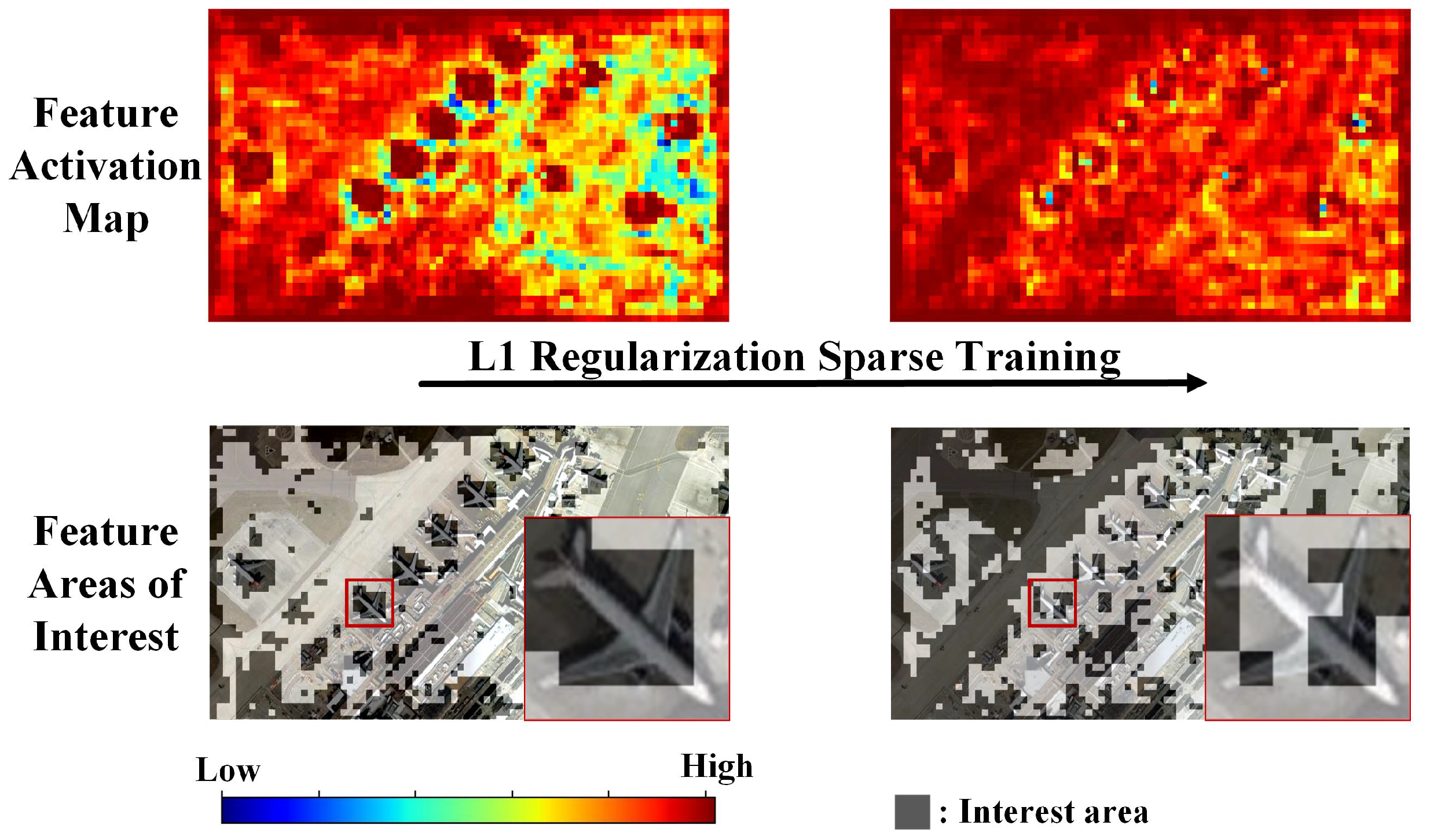
As shown in Figure 1, the feature activation map displays regions of high attention in dark red and regions of low attention in dark blue. The background image in the feature areas of interest is the input optical remote-sensing image, with the shaded areas representing regions of high attention in the feature activation map. At the beginning of sparse training, the feature areas of interest indicate that the region of interest for this feature channel is concentrated on the airplane target. After sparse training with L1 regularization, the feature areas of interest show that the region of interest for this feature channel shifts mainly to the background, with the attention on the airplane target decreasing. This indicates that directly applying L1 regularization to sparsity in remote-sensing image object-detection models tends to focus on a significant amount of background features, leading to the loss of target features and confusion between background and target feature channels.
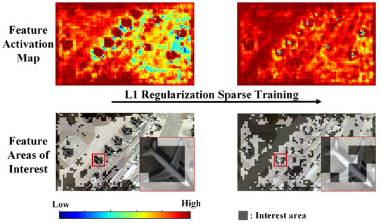
Figure 1.
Comparison of changes in the feature activation map and the feature areas of interest map of the same feature channel during L1 regularization.
References [4,5,6] used fine-tuning and knowledge distillation to improve the feature extraction performance of the model and prevent feature loss. However, the model lost features during sparse training and pruning. Therefore, this paper uses the feature attention loss () in the detection layer to represent the degree of loss of the target features during model pruning. It is defined as follows:
where D represents the input dataset; k represents the number of images in the dataset; represents the summation function of the tensor; F represents the feature activation value of the detection layer; M represents the target region mask; and c represents the number of model detection layers. Equation (1) calculates the feature attention of the detection layer on the target by computing the mean activation in the target region, reflecting the model’s attention to target features. Equation (2) then calculates the change in feature attention between the pruned model and the sparse model at each detection layer, measuring the effectiveness of the target features in the pruned model.
As shown in Figure 2, the relationship between various pruning ratios and target feature information is illustrated. In the feature activation map, regions of high attention are depicted in dark red, while regions of low attention are depicted in dark blue. Each column represents the same feature channel under different feature attention losses () for the two columns of feature activation maps. The percentage in red text represents the at that pruning rate. The zoomed-in areas in the feature activation map correspond to the zoomed-in airplane target in the input image. When the is only 0.36%, the two feature activation maps shown maintain a high level of attention on the airplane target. When the is 28.6%, the attention to the airplane target in the two feature activation maps is relatively reduced but still retains some target feature information. When the reaches 45.75%, the attention to the airplane target in the two feature activation maps is almost entirely lost.
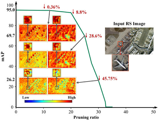
Figure 2.
Feature activation maps of the pruned model in remote sensing scenarios based on L1 regularization. In the feature activation map, regions of high attention are depicted in dark red, while regions with low attention are in dark blue. The percentage in red text represents the feature attention loss () at that pruning rate. The zoomed-in areas in the feature activation map correspond to the zoomed-in airplane target in the input image.
Therefore, the feature attention loss can measure the loss of target features. When the feature attention loss is around 1%, it can be considered that the pruned model essentially retains the target feature information of the sparse model. Conversely, if the feature attention loss is higher, it indicates a loss of target features in the pruned model.
Residual learning can enhance the model’s feature extraction ability [7], learning ability, and generalization performance. However, pruning affects the summation of feature channels in residual models. References [8,9,10,11] used the OR method in a residual model, and Reference [6] did not prune the model. Neither approach provides a balance between model size and accuracy.
To address the above issues, the L1RR was proposed to retain the feature information of remote sensing targets and achieve a balance between model size and accuracy. The implementation of L1RR has the following key steps. First, the scaling factors in the BN layer are the criterion for feature channel importance. No other parameters are required. The magnitude of these scaling factors reflects the significance of the respective feature channels and indicates the quantity of target feature information encapsulated within each channel. Second, the dynamic and self-adaptive sparsity method based on L1 is used for the remote-sensing target-detection model. This is achieved through the dynamic sparse module (DSM), which dynamically tunes the sparsity stride of each feature channel based on the amount of remote-sensing target information. Furthermore, the self-adaptive sparse module (SASM) adapts the overall sparsity stride of each layer according to variations in the number of channels containing remote-sensing target information. Third, pruning masks are constructed using scaling factors, with feature channel pruning for the remote-sensing target-detection model. The residual reconstruction procedure (RRP) is proposed to eliminate redundant features from the residual structure. It achieves forward propagation inference of pruned residual structures by reorganizing feature maps within the residual structure, utilizing both output channel recombination (OCR) and input channel recombination (ICR) methodologies. Finally, the proposal of feature attention loss as the cut-off condition in model pruning ensures the effectiveness of target features in the pruned model. This is verified by comparing the differences in target attention between the pruned model and the sparse model.
The proposed method uses the YOLOv5s model to compare the latest target detector and pruning methods on NWPU VHR-10 [12] and RSOD [13] datasets. The experimental results show that the proposed pruning framework outperforms the other methods in terms of the pruning ratio and detection accuracy.
The contributions of this paper are as follows:
- The proposed dynamic and self-adaptive sparsity method enhances model efficiency by controlling sparse ratios with DSM for the channel aspect and SASM for the layer aspect, respectively. In this way, the effective target features are given lower pruning factors and keep the training procedure away from over-sparsity.
- A new model pruning strategy is proposed, using feature attention loss as the criterion to find the balance point between the pruning ratio and accuracy. Other than enumerating the pruned ratio to find a trade-off model, the supplies a new direct metric for measuring target attention differences among original and pruned models, thereby ensuring the pruned model’s performance and reliability.
- A residual reconstruction procedure method is proposed, which only alters forward propagation with effective logical rules and pruning factors, resulting in compact and practical residual features.
The rest of this paper is organized as follows. Section 2 describes the related work on deep learning-based pruning of target detection models for remote sensing applications. The proposed method for target detection model pruning is described in Section 3. Section 4 describes the experiment and results. Section 5 describes the ablation study. Section 6 concludes the paper.
2. Related Work
2.1. Remote-Sensing Target Detection
One-stage target-detection algorithms perform target location and classification simultaneously. Two-stage target-detection algorithms first detect the candidate region where the target may exist and then classify the candidate region and target position [14].
The former algorithms have better real-time performance and are more suitable for deployment on edge computing platforms. You only look once (YOLO) [15] was the first one-stage target detection model, achieving end-to-end optimization. YOLOv2 [16] improved the original model by introducing anchor and batch normalization. YOLOv3 [17] was an improved model through a more efficient backbone network and spatial pyramid pooling. YOLOv4 [18] and YOLOv5 [19] inherit the advantages of YOLOv3 and have an optimized model structure, improving the detection performance. YOLOX [20] is an anchor-free one-stage target-detection model that improves upon YOLOv3 by adding optimization algorithms such as data augmentation, decoupled head, and Similarity Overlap Threshold Assigner (SimOTA), providing a lightweight model suitable for multi-scale analysis. PP-YOLOE [21] is an anchor-free one-stage target detector with a more efficient dynamic matching strategy and task-aligned head. A unified model structure is used to enable multi-scale analysis. YOLOv7 [22] is an anchor-based model optimized for real-time target detection. The model has a coarse-to-fine label assignment strategy. It includes a new model reparameterization module and uses a concatenation-based scaling method to improve efficiency and enable multi-scale target detection. YOLOv8 [23] is a lightweight model for multi-scale target detection based on an anchor-free architecture. The model replaces the C3 module in the YOLOv5 model with a more lightweight C2f module and uses a decoupled head and task-aligned assigner for sample matching.
Most target-detection networks for remote-sensing images have improved detection networks to achieve better performance. R-YOLO [24] contains an MS transformer module based on YOLOv5 and a convolutional block attention module (CBAM) to enhance the network’s feature extraction capability. The priori frame design of YOLOv5 was improved to make it suitable for detecting targets in rotated images. SPH-YOLOv5 [25] uses Swin-transformer prediction heads (SPHs) and normalization-based attention modules (NAMs) to improve the detection accuracy for small targets in satellite images. ECAP-YOLO [26] has a high detection accuracy for small targets and low computational complexity because it reduces model depth by leveraging shallow features for detecting small targets. CSD-YOLO [27] combines spatial pyramid pooling and a shuffle attention mechanism with a feature pyramid network (SAS-FPN) based on YOLOv7, improving the loss function and the model’s performance for detecting ships in synthetic aperture radar (SAR) images.
Although existing one-stage target-detection models have a high accuracy for remote-sensing target detection, many parameters and FLOPs limit the inference time in edge computing platforms. The coarse-grained lightweight implementations do not balance the model’s size and accuracy.
2.2. Pruning of Remote-Sensing Target-Detection Models
Unstructured and structured pruning methods exist. Unstructured pruning, also known as fine-grained pruning, refers to the pruning of unstructured modules such as weights. This strategy significantly affects model inference speed while maintaining accuracy. Structured pruning, also known as coarse-grained pruning, refers to the pruning of structured modules such as feature channels. This method retains some of the redundant weight parameters and significantly improves model inference and hardware acceleration.
Several methods have been used recently for target detection model pruning, including NS [2], soft filter pruning (SFP) [28], and performance-aware global channel pruning (PAGCP) [29]. NS utilizes the scaling factor of the BN layer to perform L1 sparse training and differentiate the importance of the feature channels. SFP uses a criterion and a layer pruning ratio to perform soft pruning and model training to differentiate the importance of the feature channels. PAGCP uses sequentially greedy channel pruning based on a performance-aware oracle criterion. It can prune multi-task models without sparse regularization.
The NS method has advantages in flexibility and simplicity of implementation because it uses feature-channel-level pruning. Additionally, the method does not require a sparse regularization of model weights, making it widely applicable for pruning target-detection models.
Most remote-sensing target-detection models use NS to increase the inference speed and reduce model complexity to facilitate the deployment on hardware platforms. Light-YOLOv4 [11] prunes unimportant channels and layers using NS pruning, reducing the network size, improving accuracy, and increasing inference speed. Ghost-YOLOS [30] prunes the YOLOv3 model using NS pruning to facilitate field-programmable gate array (FPGA) hardware acceleration. The model utilizes knowledge distillation to compensate for accuracy degradation due to pruning and is deployed on the FPGA after quantization. Lite-YOLOv5 [31] reduces the number of parameters and computational complexity of the YOLOv5 model. It prunes the YOLOv5 model using NS and uses fine-tuning to compensate for accuracy degradation caused by pruning.
NS pruning is widely used in remote-sensing target detection to reduce the number of model parameters. However, this method does not consider the feature loss that may occur during sparse training and pruning. This paper aims to balance model size and accuracy in target detection. Therefore, we optimize the L1 sparse regularization of the feature channel and layer dimension to increase the ability to distinguish meaningful channels. Additionally, we use to determine the effective pruning ratio.
3. Methodology
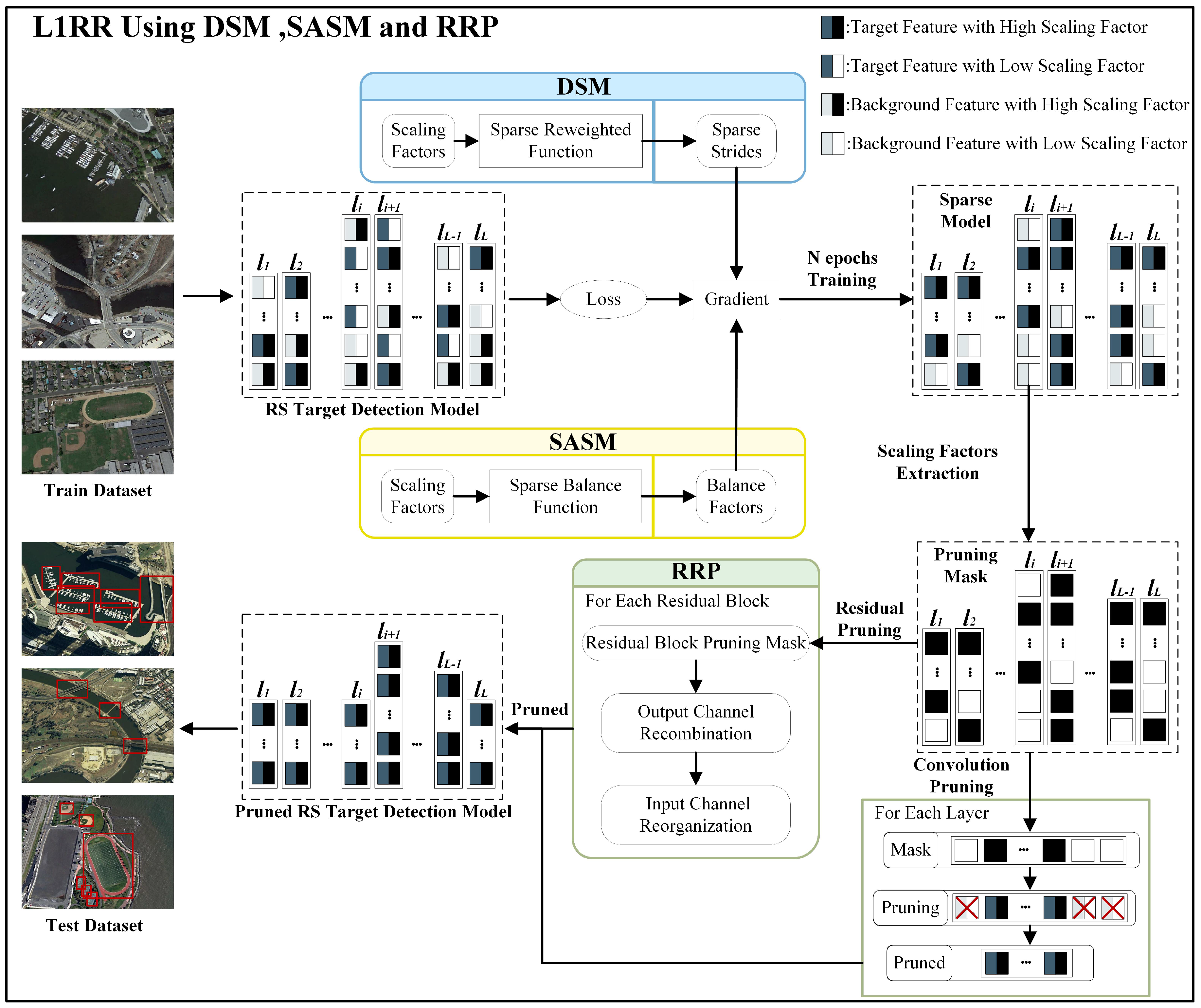
Figure 3 shows the L1RR framework. It consists of three modules: DSM, SASM, and RRP. It is implemented as follows:
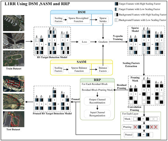
Figure 3.
Block Diagram of L1RR.
Firstly, the DSM is used to dynamically adjust the model sparsity in the feature channel dimension through sparse strides, allocating larger sparse strides to background feature channels and smaller sparse strides to target feature channels. By dynamically adjusting sparse strides in feature channels, it enhances the distinguishability of feature channels and minimizes the likelihood of target feature loss. The SASM is employed to adjust the model sparsity in the layer dimension adaptively through balance factors. It decreases the sparsity rate for layers with higher sparsity levels and increases the sparsity rate for layers with lower sparsity levels. This adaptive adjustment of layer sparsity rates prevents over-sparsity of layers, which could lead to the loss of target features. Sparse training of the DSM and SASM are used. The target-detection model assigns a high scaling factor to the target feature channel and a low scaling factor to the background feature channel. The sparse model is obtained after N epochs of training, resulting in the ability to distinguish target features from background features.
Secondly, feature channels with high scaling factors (black rectangles) are retained while those with low scaling factors (white rectangles) are pruned by constructing a pruning mask for the sparse model to extract the scaling factors.
Thirdly, the sparse model is pruned using the pruning mask. Convolutional pruning is applied to prune the feature channels, except for the residual structure. RRP is used to prune the feature channels for the residual structure. It utilizes OCR and ICR to remove redundant channels through model pruning. Convolutional pruning and RRP prune the sparse model, resulting in the final pruned target-detection model. Finally, feature attention loss is used to test the effectiveness of the target features in the pruned model.
3.1. Dynamic Sparse Module and Self-Adaptive Sparse Module for Sparse Training
3.1.1. Dynamic Sparse Module
Due to small targets and a large proportion of background information in remote-sensing images, L1 sparse regularization with a fixed stride can result in target feature loss.
Thus, reweighted L1 regularization [32] is utilized to obtain dynamically adjusted weights in addition to L1 sparse regularization, ensuring that each element has a sparsity ratio. The sparse reweighted regularization is formulated as follows:
The sparse reweighted function is formulated as follows:
where is a positive weight; denotes the of the t-th update, initialized with ; and denotes L1 regularization.
The sparse training is divided into n phases, each consisting of t epochs. At the start of training, is initialized to 0, which is equivalent to normal model training for t epochs. is updated at the beginning of the 2nd phase to perform sparse training. Subsequently, a new round of updates occurs at the beginning of the 3rd phase, and so on, until the end of training.
3.1.2. Self-Adaptive Sparse Module
Since remote-sensing images are dominated by small targets, shallow rather than deep feature maps are commonly used because they contain more information on small targets. However, the traditional method for achieving sparsity is to apply a uniform sparsity level to the model. This approach can result in excessive sparsity of shallow features, causing feature loss and a low model accuracy.
Therefore, we propose an adaptive sparse module based on the exponential function. This module adjusts the sparsity degree layer-by-layer by considering the difference in the layer sparsity degree. The objective is to prevent feature loss caused by over-sparsity. Additionally, experiments have shown that a scaling factor of less than 0.01 has a negligible impact on the model’s detection performance. The model’s sparsity degree is the ratio of the number of scaling factors of less than 0.01 to the total number of scaling factors.The sparsity of the current layer is the ratio of the number of filters with a scaling factor of less than 0.01 to the total number of filters. The sparse balance function is formulated as follows:
where is an exponential function with a base of two, denoting the sparse balance factor of the i-th layer; t denotes the balance factor of the t-th update; initialization occurs with ; and t does not exceed 10; a is a hyperparameter to adjust the intensity of the change in the balance factor; denotes the current sparsity of the model; and N denote the number of pruned filters and the total number of filters in the current layer, respectively.
Since filters are more important in shallow than deep networks, the feature extraction ability of shallow networks is affected by the sparsity constraint. Thus, we propose a -decay strategy. It is used when the sparsity of a layer remains unchanged for a long time during sparse training:
where s denotes the number of times the layer is very sparse.
3.1.3. Dynamic and Self-Adaptive Sparsity
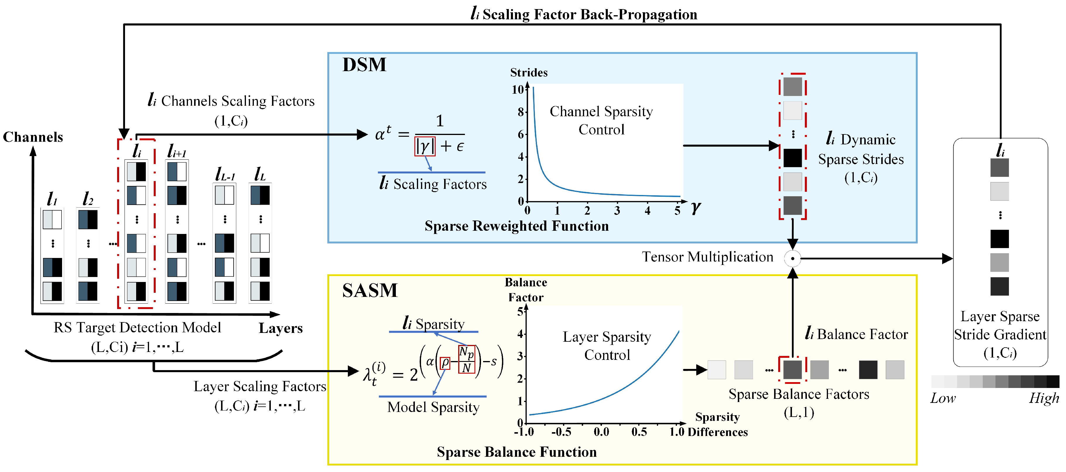
Figure 4 illustrates the implementation of the DSM and SASM to optimize model sparsity. For instance, in layer i, the sparsity optimization for the target detection model is as follows:
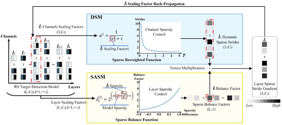
Figure 4.
The single-layer sparse stride gradient construction. The color shades of the squares represent the weights. Darker colors indicate larger weights, while lighter colors indicate smaller weights.
In the first step, the scaling factor of the layer i’s channel dimension is input into the sparse reweighted function in the DSM. Dynamic sparse strides are generated from the feature channel dimension. DSM assigns larger sparse strides to background feature channels and smaller sparse strides to target feature channels, increasing the distinguishability between feature channels and preventing the loss of target features. The scaling factor in the layers is input into the sparse balance function in the SASM, generating the balance factor from the layer dimension. SASM reduces the sparse stride for layers with sparsity higher than the model’s overall sparsity and for layers where sparsity is saturated, while increasing the sparse stride for layers with sparsity lower than the model’s overall sparsity, preventing over-sparsity from causing the loss of target features.
In the second step, the layer’s sparse stride gradient (LSSG) of layer i is obtained by tensor-multiplying the dynamic strides and the balance factor of layer i. The LSSG and the training gradient are used to adjust the scaling factor of layer i through back-propagation. This approach enables cooperative sparsity control of feature channels and layers, increasing the distinguishability of feature channels and decreasing the likelihood of losing target features.
Sparse training is performed using DSM and SASM with the LSSG to achieve model sparsity. The sparse gradient is defined as follows:
where ∇ denotes the gradient; denotes the i-th layer’s scaling factors; denotes the DSM; denotes the SASM of the i-th layer; and denotes the sparsity ratio of the model.
Algorithm 1 describes the sparse training
| Algorithm 1 Sparse Training Process |
|
3.2. Model Convolution Pruning and Residual Reconstruction Procedure
The resulting sparse model undergoes feature channel pruning to obtain a pruned model. The sparse model is defined as follows:
The pruned model is expressed as follows:
where and denote the sparse and pruned models, respectively; and denote the weight tensor and the pruned weight tensor of the i-th layer, respectively; denotes the number of output channels for the i-th layer; denotes the number of input channels for the i-th layer; denotes the number of output channels after pruning for the i-th layer; denotes the number of input channels after pruning for the i-th layer; denotes the size of the two-dimensional spatial kernel for the i-th layer; denotes the pruning mask for the i-th layer. does not exist when the i-th layer is the first layer; thus, only the output channels are pruned in the first layer.
There is a correspondence between the output channels of one layer and the input channels of the next layer. Therefore, the pruning process for the model’s feature channels can be described as pruning the model in both the output channel dimension and the input channel dimension. The pruned output channels can be represented as the tensor multiplication of the sparse model’s weights with the pruning mask from the output channel dimension (), while the pruned input channels can be represented as the tensor multiplication of the sparse model’s weights with the pruning mask from the previous layer’s input channel dimension ().
During model pruning, threshold screening is conducted to obtain the scaling factor of the BN layer in each network layer. The threshold value of the pruning model is evaluated using . If the is around 1%, the pruning is considered effective. However, if it exceeds 1%, the feature information is significantly affected, and the pruning is invalid.
Furthermore, the residual structure of the target detection model can be difficult to prune. The original residual structure is depicted in Figure 5. The outputs of and must be summed in the same dimension and require the same pruning mask. However, and typically have different pruning masks.

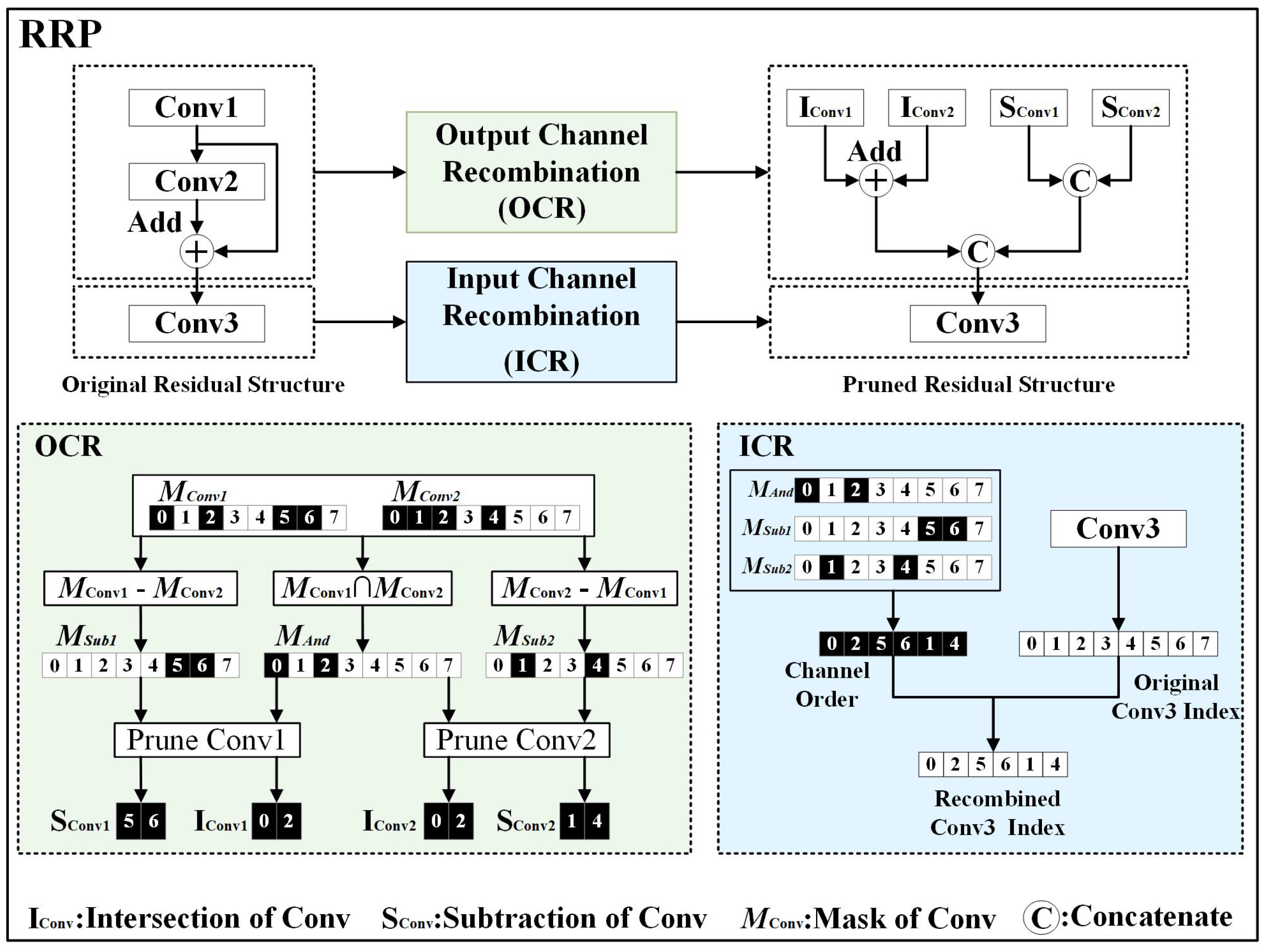
Figure 5.
Schematic diagram of residual reconstruction procedure.
Figure 5 shows the proposed RRP. It consists of OCR and ICR. , , and represent different convolutional layers, with and forming a residual structure. M denotes the mask, where black squares indicate a mask value of 1, white squares indicate a mask value of 0, and the numbers within the squares represent channel indices. The main steps of RRP are as follows:
First, OCR uses the pruning mask for and the pruning mask for to obtain using an intersection operation. is used to prune the residual structure while preserving the original additive channels and . is obtained by subtracting from . It is used to compute the channels in that cannot be added, resulting in . is derived by subtracting from . It is used to compute the channels in that cannot be added, resulting in . The resulting and are used to prune , producing the pruned channels and for . and are used to prune , producing the pruned channels and for . and are summed, and and are concatenated. The results of the summing and concatenation are the input for .
ICR utilizes three pruning masks (, , and ) obtained from OCR to determine the output channel order of the residual structure’s output feature maps. This channel order is then used as the pruning mask for the input channels of the next layer’s , resulting in a new .
The RRP does not consider convolutional layers with the same pruning mask; thus, the pruned model has the same accuracy but fewer parameters. The output of the is expressed as follows:
The output of the is expressed as follows:
The output of the residual structure is expressed as follows:
The correspondence between the output feature maps is no longer one-to-one due to differences in pruning masks. We use the pruning mask to address this. We obtain the pruning mask for the ’s feature map and the pruning mask for the ’s feature map of the residual module. Intersection and subtraction ( and ) operations are performed. The output feature map of the residuals is expressed as follows:
After the output feature maps of the residuals have been combined, it is necessary to reorder the inputs of the kernels/filters in the next layer using the channel order. The pruning structure of the next layer’s kernels/filters of the residual structure is expressed as follows:
where denotes the mask of the channel order after reconstruction.
The pruning process is defined in Algorithm 2.
| Algorithm 2 Pruning Process |
|
4. Experiment
Experiments were conducted using the proposed pruning framework to verify its effectiveness. Two remote-sensing datasets and the YOLOv5s model were used. This section describes the two remote-sensing datasets, the NWPU VHR-10 and the RSOD datasets. The implementation details, including the training strategy and evaluation metrics, are presented. The accuracy, detection speed, and model size of the proposed and other lightweight networks are compared. The accuracy, parameter pruning ratio, and FLOP pruning ratio of the proposed and other pruning methods are contrasted.
4.1. Datasets
The NWPU VHR-10 dataset [12] is a geospatial target-detection dataset containing ten categories with image sizes of 600 × 600 to 1100 × 1100. The target classes include airplane (PL), ship (SH), storage tank (ST), baseball diamond (BD), tennis court (TC), basketball court (BC), ground track field (GT), harbor ( HA), bridge (BR), and vehicle (VH). The dataset has 650 labeled images. We used 80% of the images for training and 20% for testing.
The RSOD dataset [13] is a geospatial target-detection dataset containing four categories: aircraft, oiltank, overpass, and playground. The dataset has 936 images. Similarly, an 80%/20% training/testing ratio was used.
4.2. Implementation Details
4.2.1. Training Strategy
Nearly identical training strategies were used for the two datasets. The anchor-based object detector YOLOv5s model with version 6.1 was utilized. Table 1 shows the anchor settings of the YOLOv5s model, customized to align with the sizes and distributions of targets in the remote-sensing datasets using the k-means clustering method. A stochastic gradient descent (SGD) was employed to optimize the loss function during training. The training epoch was 300, with a sparsity rate of 0.001, a learning rate of 0.01, a warm-up learning rate of 0.001, and 1000 iterations. The dynamic adaptive updating epoch was 40. The non-maximum suppression intersection over union (IoU) threshold during testing was 0.6, and the confidence threshold was 0.001.

Table 1.
The anchor settings of the YOLOv5s model.
4.2.2. Evaluation Metrics
Several metrics were used to assess the target detection model’s performance: mean average precision (mAP), number of parameters (Params), number of FLOPs, frames per second (FPS), Parameter Prune Ratio (), and FLOP Prune Ratio ().
The mAP is based on recall and precision. The true positive (TP), false positive (FP), and false negative (FN) are calculated. A TP occurs when the overlap ratio of the predicted box and ground truth exceeds a given threshold. Conversely, an FP occurs when the overlap ratio is lower. An FN occurs if there is no match between the prediction and ground truth. The equations for recall and precision are as follows:
The area below the precision–recall (P-R) curve is the average precision (AP), and the mean of the APs of all categories is the mAP:
The equations for and are as follows:
The mAP is a measure of the detection accuracy of the target-detection model. Params, FLOPs, and FPS are used to measure the complexity and detection speed of the target-detection model. and are used to measure the pruning performance.
4.3. Results
4.3.1. Target-Detection Model Results
We pruned the YOLOv5s model and compared it with other models and the proposed model on two remote-sensing datasets.
Table 2 depicts the results of the proposed model and the latest lightweight target-detection model on the NWPU VHR-10 dataset. The comparison focuses on the target category accuracy, mAP, model size, and FPS. Optimal values in each category are indicated in bold.
Table 2.
Detection results on the NWPU VHR-10 dataset.
The pruned model achieved an mAP of 95.0%, significantly higher than the other models. Compared to object-detection models designed for natural scenes, it achieved a 2.6% and a 8.2% higher mAP than that of the large target detection models YOLOv3 [17] and Faster R-CNN [37], respectively. Additionally, the model size was reduced by 97.3% and 98%. The pruned model achieved 2.8% and 0.7% higher mAPs than the latest lightweight models YOLOv7-tiny [22] and YOLOv8n [23], respectively. Additionally, the model size was reduced by 64.5% and 24.8% for single-precision floating-point storage. It also exhibited a significantly higher FPS than both. Compared to the remote-sensing object-detection models, the pruned model achieved 4.2% and 1.7% higher mAPs than the latest optical remote-sensing models LAR-YOLOv8 [36] and CANet [38], respectively. Furthermore, the pruned model was only 23% the size of the baseline model. On NVIDIA Jetson TX2, the pruned model had a 48.5% higher model inference speed than the baseline model.
Although the overall detection accuracy of the pruned model was 0.1% that of the baseline model, the accuracy for ship and vehicle targets was 5.2% and 5.1% lower, respectively. However, the accuracy of detecting harbor and bridge targets was 4.2% and 7.9% higher, respectively, while that of the remaining targets remained unchanged. The model’s detection accuracy fluctuated due to the removal of redundant features in the baseline model during sparse modeling. The pruned model had the same target-detection accuracy as the baseline model for small targets and a significantly higher accuracy for large targets, such as bridges and harbors.
The proposed pruning framework does not require pre-training or fine-tuning; thus, the regularization constraints are implemented during sparse training. This can cause differences in the detection accuracy of certain targets; however, the detection accuracy was comparable to that of the baseline model.
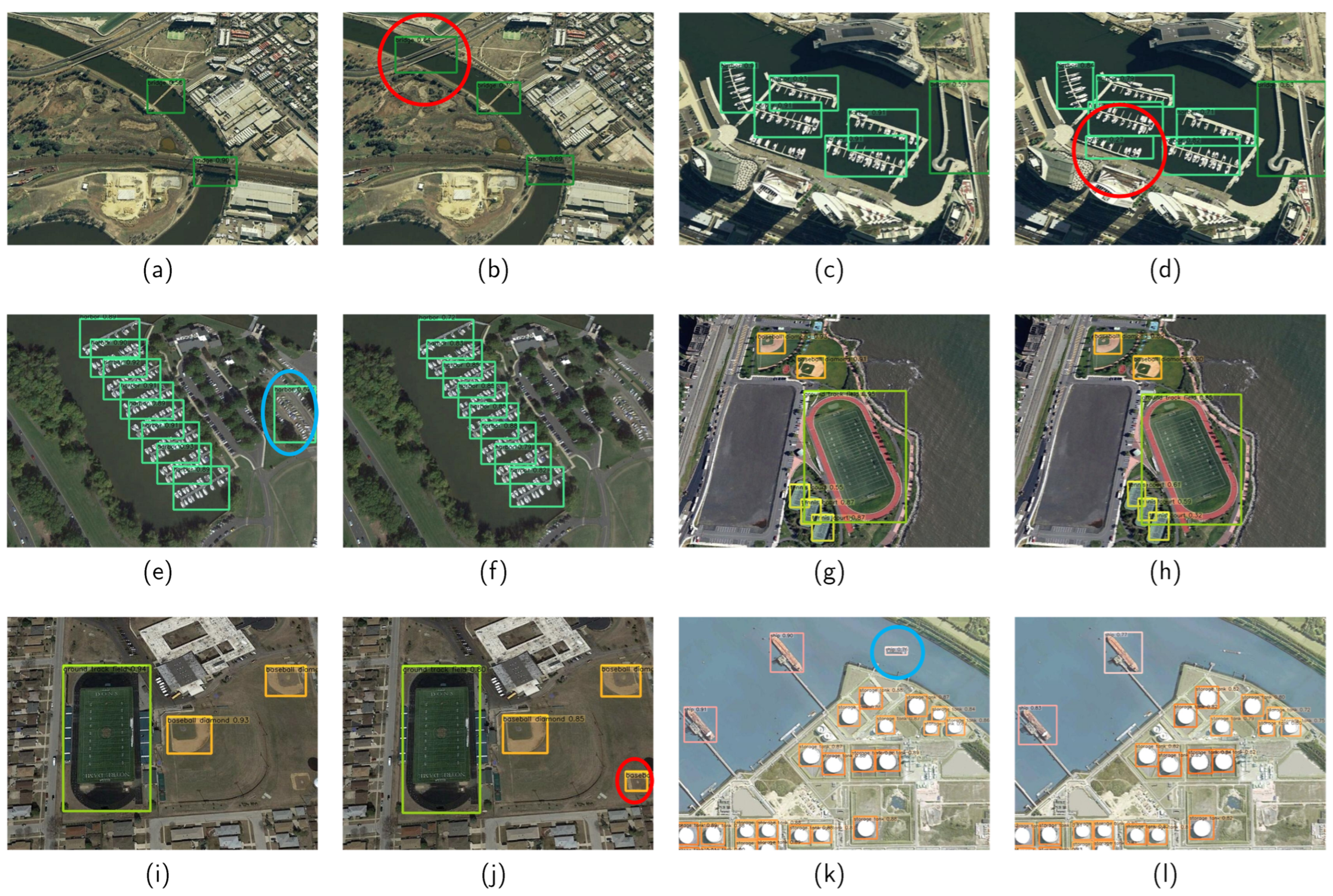
Figure 6 compares the detection results of the baseline (a,c,e,g,i,k) and pruned (b,d,f,h,j,l) models on the NWPU VHR-10 dataset. In Figure 6a,b, the baseline model missed the bridge target, whereas the pruned model correctly identified it. In Figure 6c,d, the baseline model missed the harbor target, while the pruned model correctly detected it. Figure 6e,f show that the baseline model had a false alarm for the harbor target, whereas the pruned model correctly detected all targets without false alarms. Similarly, the baseline model had a missed detection for the baseball diamond target, while the pruned model correctly detected it (Figure 6i,j). Figure 6k,l indicate that the baseline model incorrectly identified a ship (false alarm), whereas the pruned model correctly identified this area as the background.
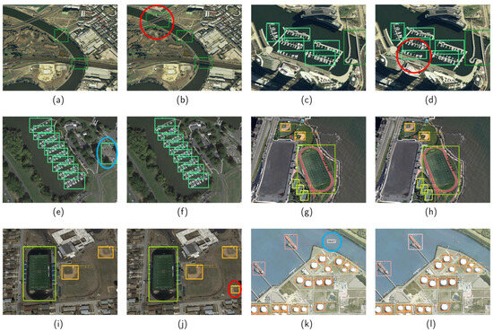
Figure 6.
The detection results for the baseline (a,c,e,g,i,k) and pruned (b,d,f,h,j,l) models on the NWPU VHR-10 dataset. The red circles represent targets detected by the pruned model but not by the baseline model, and the blue circles represent false alarms for the baseline model.
The pruned and baseline models provided similar detection results in various complex scenarios. However, the pruned model had a higher detection accuracy for bridges ((a) and (b)) and harbors ((c) and (d), (e) and (f)) in some detection scenarios.
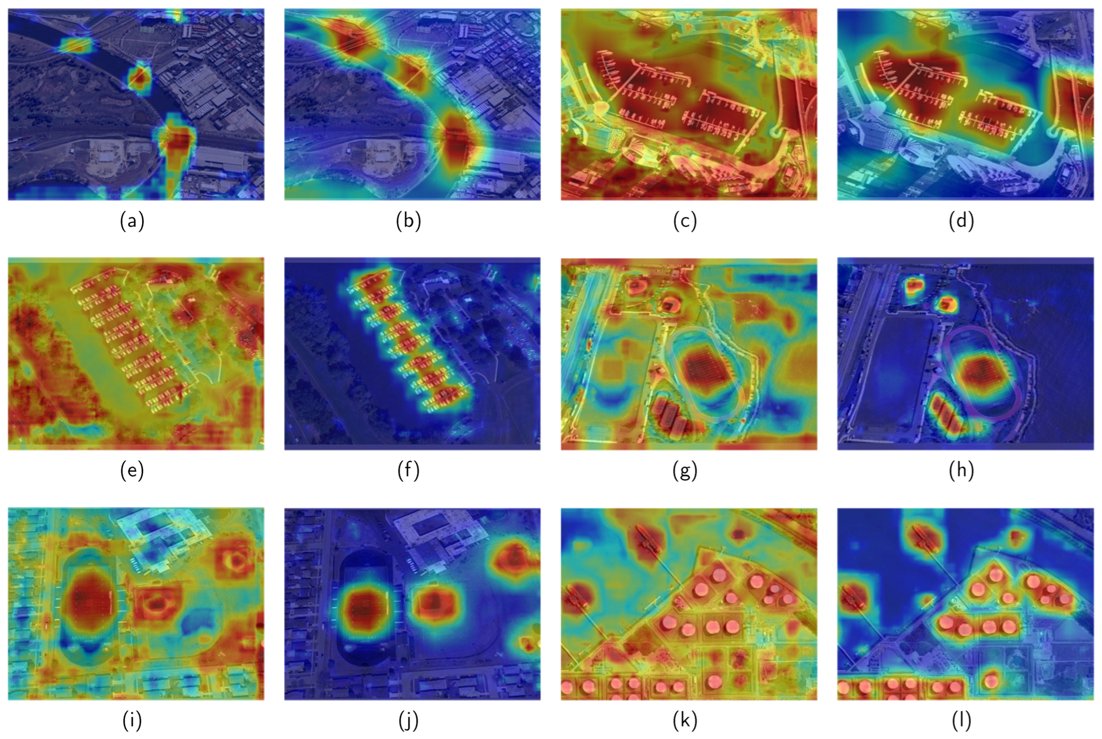
Figure 7 shows the heatmaps derived from Grad-CAM++ [40] for the baseline (a,c,e,g,i,k) and pruned (b,d,f,h,j,l) models on the NWPU VHR-10 dataset.
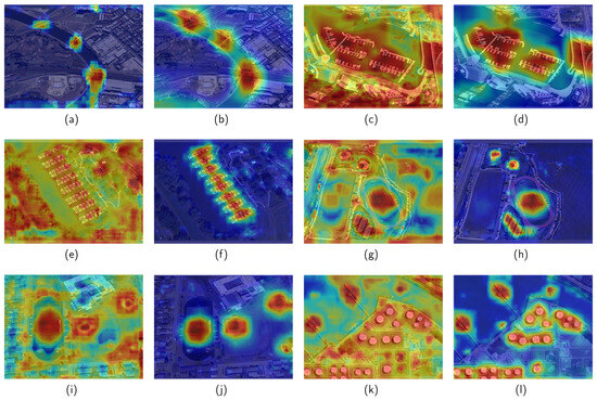
Figure 7.
The heatmap derived from Grad-CAM++ for the baseline (a,c,e,g,i,k) model and pruned (b,d,f,h,j,l) model on the NWPU VHR-10 dataset.
The baseline model focused on the target and background features, resulting in false alarms and missed detection. Figure 7a,b show that the baseline model detected bridge targets by focusing on the features of the target area. However, due to low attention to the target features, it classified the target as the background in some cases and missed some targets. In contrast, the pruned model detected all three bridge targets correctly. As shown in Figure 7c,d, the baseline model focused more on the background, resulting in missed detection. In contrast, the pruned model focused on the harbor and bridge targets and was not influenced by the background information, resulting in the correct detection of all targets. Figure 7e,f show that the baseline model’s attention was primarily focused on the background, leading to false alarms. In contrast, the pruned model focused more on the harbor target and was not influenced by the background information, correctly detecting all targets. Figure 7i,j show that the baseline model’s attention was on the target and its edges, resulting in missed detection in complex backgrounds. In contrast, the pruned model focused primarily on the target and was unaffected by the background features of the target edges. In the remaining detection scenarios (Figure 7g,h,k,l), the baseline model focused on the target and the background, resulting in correct target detection, although a significant amount of irrelevant background information was considered. In contrast, the pruned model focused solely on the target.
Table 3 compares the accuracy, mAP, model size, and FPS of the latest lightweight target-detection models on the RSOD dataset. The optimal values in each category are indicated in bold.
Table 3.
Detection results on the RSOD dataset.
The pruned model achieved a 97.3% mAP with a model size of only 6.6 MB. Compared to object-detection models designed for natural scenes, the mAP was 20.1% and 4.4% higher than that of the large target detection models YOLOv3 [17] and Faster R-CNN [37], respectively. Additionally, the model size was 97.3% and 98% smaller for single-precision floating-point storage. The mAP was also 2.3% higher than that of the lightweight model YOLOv7-tiny [22]. Compared to optical remote-sensing object-detection models, the pruned model achieved 3.0% and 2.1% higher mAP than the latest optical remote-sensing models LAR-YOLOv8 [36] and CANet [38], respectively. The model size was only 23.5% of the baseline model. The inference speed on the NVIDIA Jetson TX2 was 38.2% higher than that of the baseline model.
The pruning model’s overall detection accuracy was 0.5% lower than that of the baseline model. However, it had the same accuracy as the baseline model for different complex scenes. The target accuracy was 0.9% lower for the aircraft class, 0.4% lower for the oiltank class, and 0.5% lower for the overpass class compared to the baseline model. The target accuracy of the playground class was the same. Redundant features were eliminated from the baseline model while preserving its ability to detect small targets like airplanes and large targets like playgrounds.
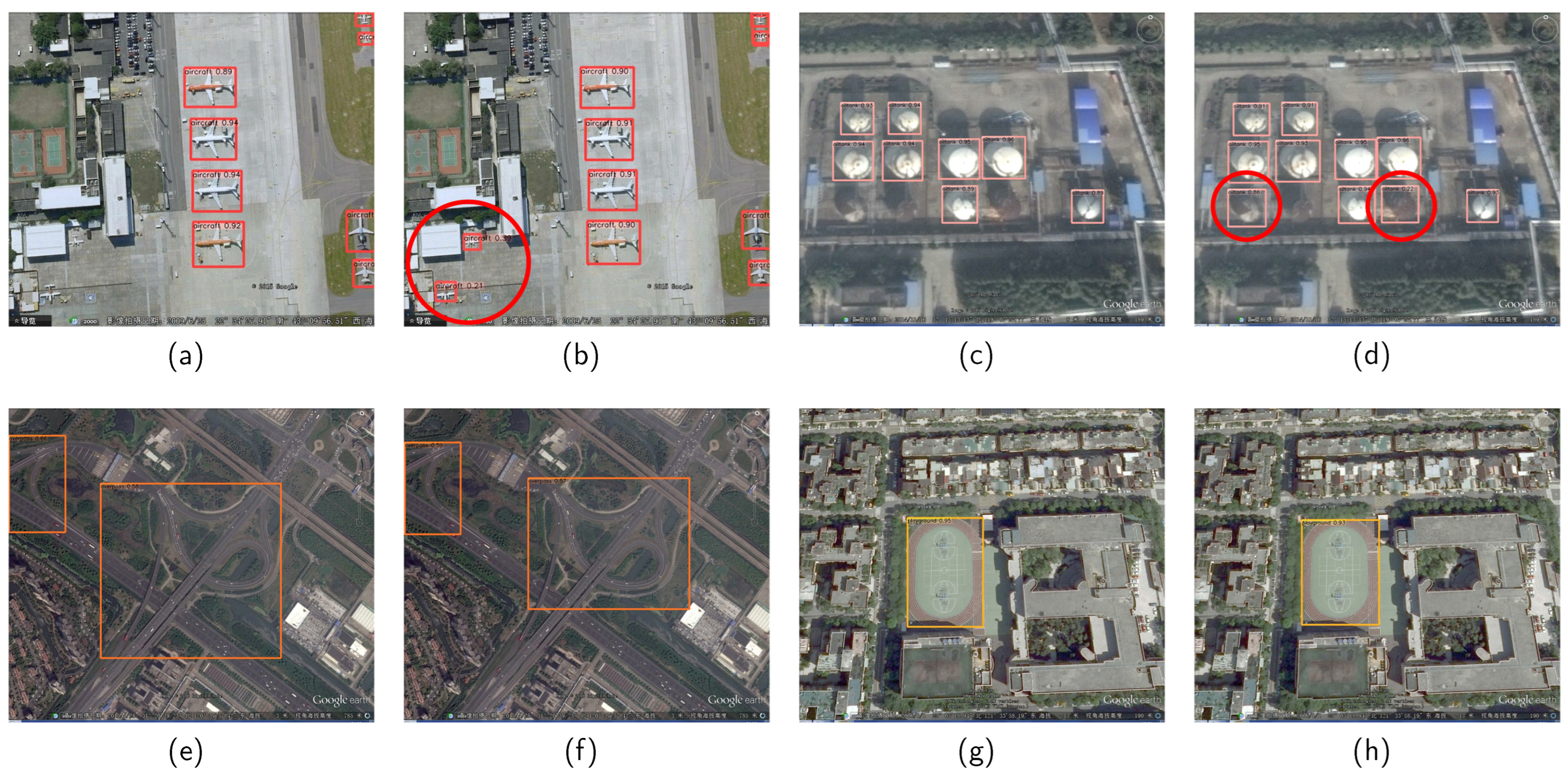
Figure 8 shows the detection results for the baseline (a,c,e,g) and pruned (b,d,f,h) models on the RSOD dataset.
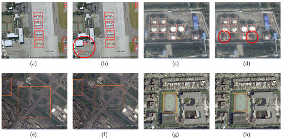
Figure 8.
Comparison of detection results for the baseline (a,c,e,g) and pruned (b,d,f,h) models in complex scenes of the RSOD dataset. The red circles indicate targets detected by the pruned model but not by the baseline model.
In Figure 8, comparing Figure 8a,b, The baseline model missed two small aircraft targets, whereas the pruned model correctly detected them. In Figure 8c,d, the baseline model missed three oiltank targets, while the pruned model correctly detected two. In the remaining detection scenarios (Figure 8e–h), the pruned and baseline models had the same detection results for large targets, such as overpasses and playgrounds.
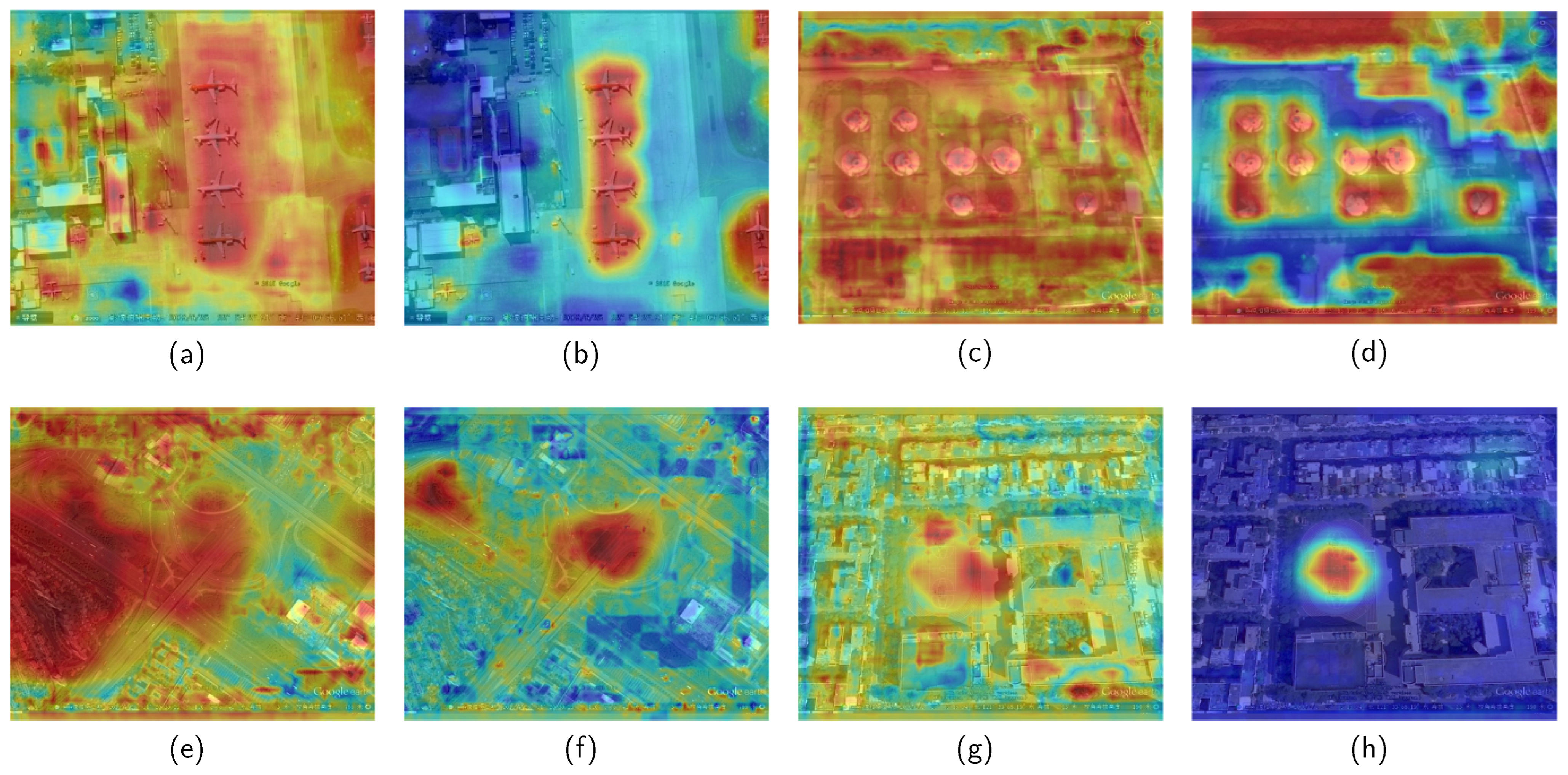
Figure 9 compares the feature heatmaps derived from Grad-CAM++ [40] for the baseline (a,c,e,g) and pruned (b,d,f,h) models on the RSOD dataset.
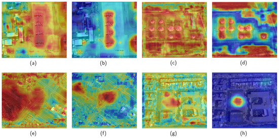
Figure 9.
The heatmap derived from Grad-CAM++ for the baseline (a,c,e,g) and pruned (b,d,f,h) models on the RSOD dataset.
The baseline model focused on target and background features in all detection scenarios. In Figure 9g,h, the baseline model had a large focus area when detecting the playground target due to the complexity of the background information. In contrast, the pruned model focused solely on the target. In the remaining detection scenarios (Figure 9a–f), the baseline model’s attention covered almost the entire image. Although it detected the target, its focus was also on the background features, resulting in missed detection. In contrast, the pruned model’s attention was primarily on the target; it detected all targets correctly.
4.3.2. Model Pruning Results
The comparison of the proposed pruning framework and other pruning methods and the performances of the YOLOv5s model and the NS [2], SFP [28], and PAGCP [29] methods on two remote-sensing datasets are listed in Table 4. The optimal values in each category are indicated in bold.
Table 4.
Comparison of L1RR and other pruning methods on remote-sensing datasets.
On the NWPU VHR-10 dataset, a comparison of the proposed high pruning ratio (>80%) model (Ours-HP) and the NS method showed that our model was 0.8% more accurate than the NS method, with a 5.83% higher parameter pruning ratio and 3.75% higher FLOP pruning ratio. To compare our model with the SFP and PAGCP methods, we used the highest-accuracy pruning model (Ours-BA) due to the low pruning ratio of SFP with PAGCP. Our model had a 3.1% higher accuracy than the SFP method, with a 25.4% higher parameter pruning ratio and a 20% higher FLOP pruning ratio. Our pruning method had a 2.58-times higher parameter pruning ratio and a 2.71 times higher FLOP pruning ratio than the PAGCP method, with almost the same accuracy.
On the RSOD dataset, our model had a 3.4% higher accuracy, a 4.84% higher parameter pruning ratio, and an 11.25% higher FLOP pruning ratio than the NS method. We compared Ours-BA with the SFP and PAGCP methods. Our model achieved 7.2% higher accuracy, a 26.25% higher parameter pruning ratio, and a 20% higher FLOP pruning ratio than the SFP method. The parameter pruning ratio was 35.83% higher, the FLOP pruning ratio was 27.5% higher, and the accuracy was 1.6% higher than for the PAGCP method. The experimental results demonstrate that our pruning method outperformed other pruning methods for the target-detection models.
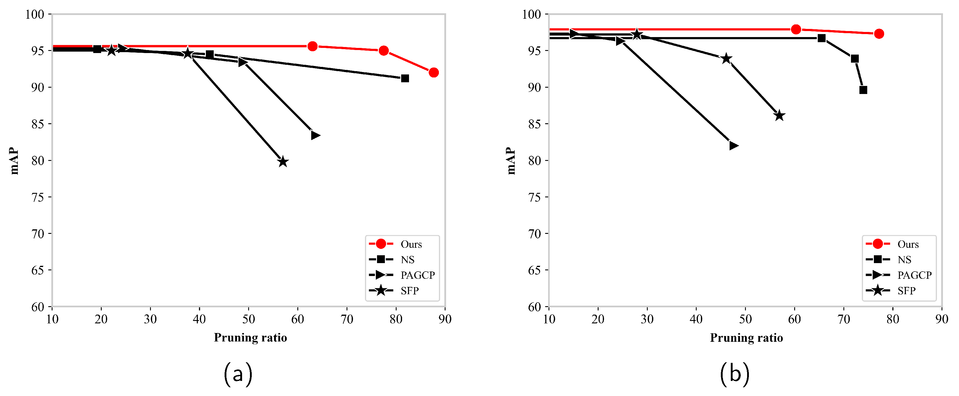
Figure 10 shows the mAP of different pruning methods for different pruning ratios. The proposed pruning framework had the highest detection accuracy and pruning ratio on the NWPU VHR-10 and RSOD datasets. The mAP of several algorithms decreased significantly and fell below 90% after the pruning ratio reached 80%. The SFP method exhibited a significant decrease in the mAP at a pruning ratio of 40%. The NS method maintained a higher accuracy, but the accuracy was below 90% when the pruning ratio exceeded 70%. In contrast, the proposed pruning framework maintained 90% and 95%, respectively.
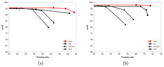
Figure 10.
Mean average precision of different pruning methods for different pruning ratios: (a) NWPU VHR-10 dataset, and (b) RSOD dataset.
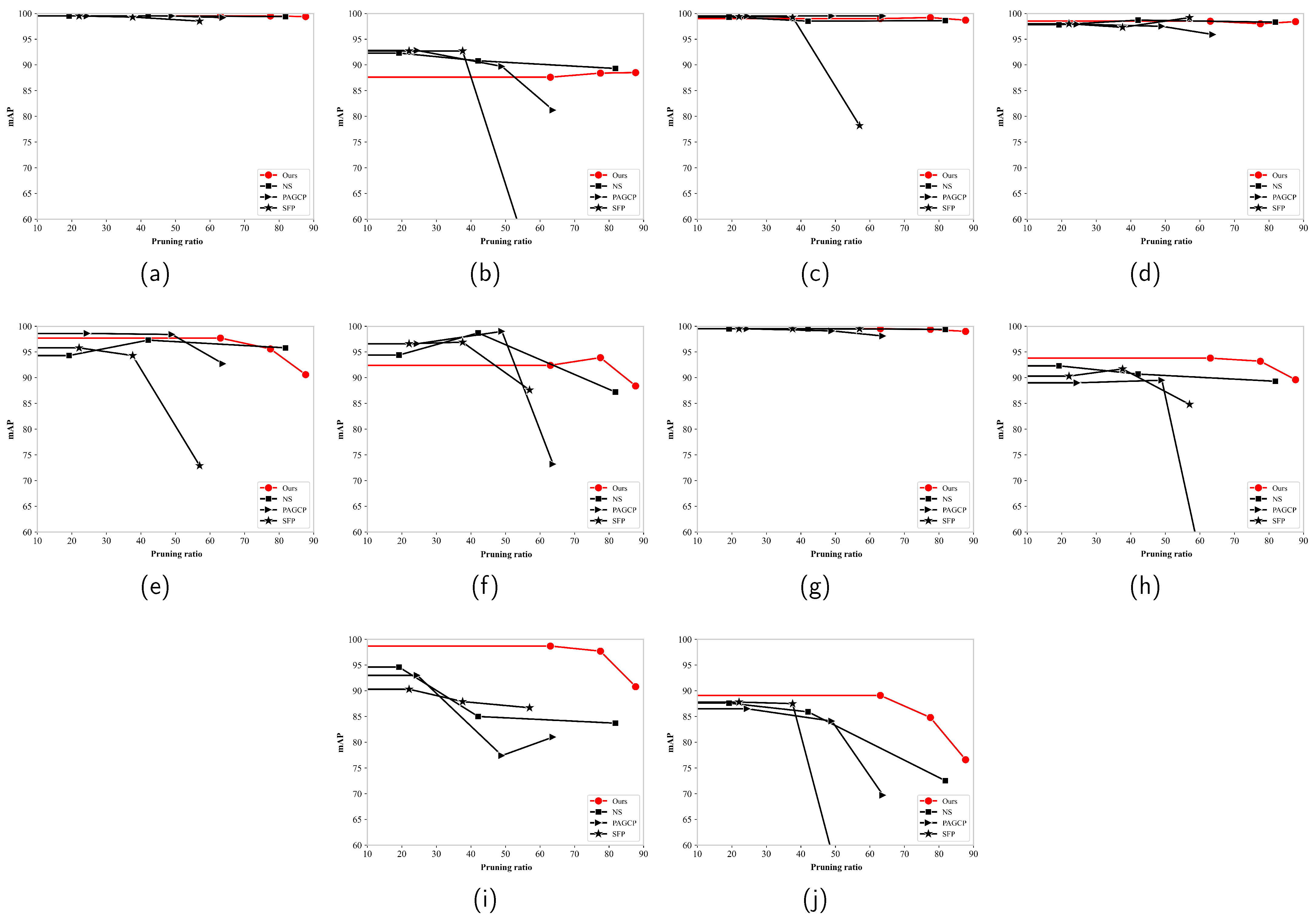
Figure 11 shows the mAP for the targets for different pruning ratios and pruning methods on the NWPU VHR-10 dataset. The mAP of several targets (ship, storage tank, and others) for the SFP method declined significantly after the pruning ratio reached 50%. The PAGCP method exhibited a significant accuracy degradation (lower than 60%) for basketball court, harbor, and other targets. Although the NS method showed a similar detection accuracy for the ship and tennis court classes compared to our method, its detection accuracy for the harbor, bridge, and vehicle classes was significantly lower than ours. Therefore, the proposed pruning framework optimally maintains target features for more targets across a wider pruning ratio range and accurately distinguishes the importance of feature channels.
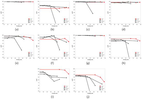
Figure 11.
Mean average precision for various targets for different pruning methods and pruning ratios on the NWPU VHR10 dataset: (a) airplane; (b) ship; (c) storge tank; (d) baseball diamond; (e) tennis court; (f) basketball court; (g) ground track field; (h) harbor; (i) bridge and (j) vehicle.
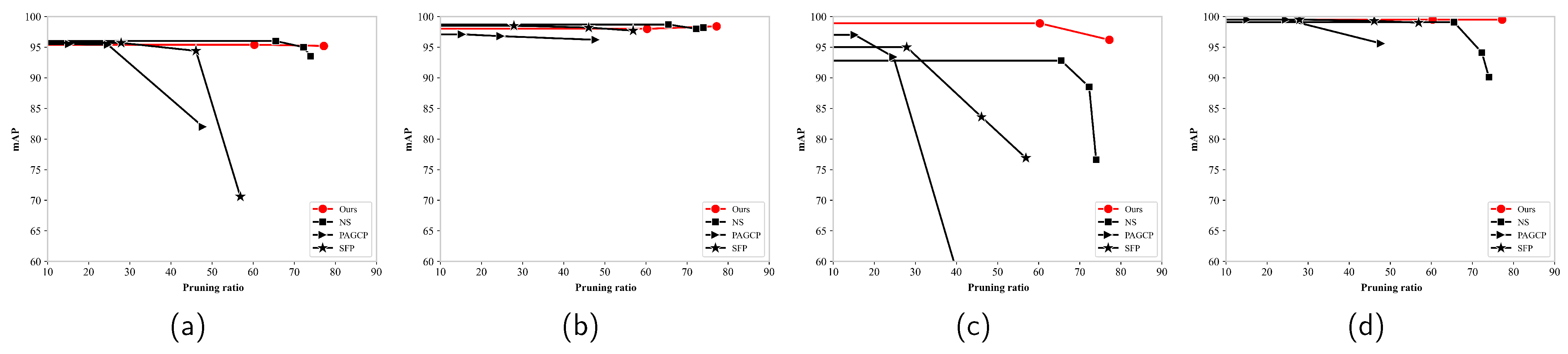
Figure 12 displays the mAP for various targets for different pruning ratios and methods on the RSOD dataset. The SFP and PAGCP methods showed significant accuracy degradation for the aircraft and overpass targets (below 60%) after the pruning ratio reached 50%. The NS method exhibited substantial accuracy degradation for all targets when the pruning ratio exceeded 70%. In contrast, the proposed pruning framework only showed a slight decrease in accuracy for the overpass target, while the accuracy remained above 95% for a wide pruning ratio range.
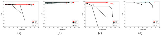
Figure 12.
Mean average precision for various targets for different pruning ratios and methods on the RSOD dataset: (a) aircraft; (b) oiltank; (c) overpass and (d) playground.
5. Ablation Study
The proposed pruning approach comprises three modules: DSM, SASM, and RRP. We conducted ablation experiments to compare the influence of different modules on the accuracy and model parameters. The following analysis was conducted.
- Sparse training of the model using only the DSM.
- Sparse training of the model using the DSM and RRP.
- Sparse training of the model using the DSM and SASM.
- The DSM and SASM are used to simplify the model and to implement RPP.
The results in Table 5 indicate that the Yolov5s model had significantly fewer parameters and the highest accuracy. The optimal values in each category are indicated in bold. Specifically, the number of parameters was reduced by 55.23% with virtually no impact on the mAP when only the DSM was used on the NWPU VHR-10 dataset. The combination of the DSM and SASM resulted in a 72.02% reduction in the number of parameters without sacrificing accuracy. The use of the DSM, SASM, and RRP resulted in a 77.54% reduction in the number of parameters while maintaining accuracy. Similar results were observed on the RSOD dataset. Using the DSM reduced the parameter count by 57.29%, with a minor decrease in the mAP. The combination of the DSM and SASM reduced the parameter count by 75.29%. Using all three modules reduced the parameters by 76.97% without compromising accuracy.
Table 5.
Results of ablation study.
The accuracy of the pruned models with different pruning ratios trained on the NWPU VHR-10 dataset and the RSOD dataset was compared. We assessed four pruning ratios, labeled as “Prune-pruning ratio”: “Prune-40” refers to the model where the feature channels were pruned by 40%. “Baseline” denotes the base training result for the YOLOv5s model. “Sparse” denotes the sparse model at the end of sparse training, with an optimum pruning ratio of 66.5% on the NWPU VHR-10 dataset and 73.2% on the RSOD dataset.
Table 6 presents the experimental results of the six models on the NWPU VHR-10 dataset. The sparse model differed slightly from the baseline model, resulting in 0.001 lower mAP@0.5. When the pruning ratio was lower than the optimal one, Prune-20 and Prune-40 exhibited no difference in mAP compared to the sparse model. Additionally, they had fewer parameters and FLOPs, and the values were low (0.25% and 0.24%, respectively). Prune-66.5 had the same mAP as the sparse model and significantly fewer parameters and FLOPs when the pruning ratio was optimal. The value was only 1.14%, and no noticeable difference in the feature extraction ability was observed compared to the sparse model. The mAP@0.5 of Prune-70 was 0.017 lower than that of the sparse model when the pruning ratio exceeded the optimal values. Although the number of parameters and FLOPs were significantly lower, the value was 6.79%, affecting the model’s feature extraction ability.
Table 6.
YOLOv5s pruning results for sparse models with different pruning ratios on the NWPU VHR-10 dataset.
Table 7 compares the performances of the six models on the RSOD dataset. The mAP@0.5 of the sparse model was 0.005 lower than that of the baseline model. Prune-20, Prune-60, and the sparse model had the same mAP when the pruning ratio was lower than the optimal one. Additionally, they had fewer parameters and FLOPs. The values were only 0.5% and 0.57%, respectively. Prune-73.2 had the same mAP as the sparse model when the pruning ratio was optimal. Additionally, the number of parameters and FLOPs were significantly lower, and the value was only 0.6%. The feature extraction abilities of the Prune-73.2 and the sparse model were similar. Prune-77 had a 0.479 lower mAP@0.5 than the sparse model when the pruning ratio exceeded the optimum value. It had fewer parameters and FLOPs. However, the high value (19.4%) indicated a low feature extraction ability.
Table 7.
YOLOv5s pruning results for sparse models with different pruning ratios on the RSOD dataset.
To validate the effectiveness of L1RR in microwave remote-sensing images, the YOLOv5 model was pruned for synthetic aperture radar (SAR) image ship detection using the high-resolution SAR images dataset (HRSID) [43]. The primary comparisons were made in terms of mAP, parameters, model size, and GFLOPs.
Table 8 shows the model pruning results for microwave remote-sensing images on the HRSID dataset. The optimal values in each category are indicated in bold. The pruned model achieved a 92.4% mAP with a model size of only 7.2 MB, resulting in a parameter pruning rate and FLOP pruning rate of 77.8% and 61.25%, respectively. Compared to object-detection models designed for natural scenes, it outperformed the large target detection model Faster R-CNN [37] by 8.4% in mAP, while reducing the model size by 98% when stored in single-precision floating-point format. Additionally, it surpassed the lightweight model YOLOX-tiny [22] by 3.7% in mAP. When compared to models designed for microwave remote-sensing scenes, the pruned model achieved a higher mAP than SAR-Net [44] and ZeroSARNas [45] by 7.7% and 1.1%, respectively. The parameters were reduced by 96.3% and 10.8%, respectively. Furthermore, compared to pruning methods NS [2] and SFP [28], the pruned model achieved a higher mAP than YOLOv5s + NS and YOLOv5s + SFP by 2.5% and 1.1%, respectively, while achieving a higher parameter-pruning rate of 13.57% and 42.9% and a higher FLOP-pruning rate of 16.25% and 30%, respectively.The experimental results demonstrate that our proposed method achieves competitive detection performance even in microwave remote-sensing scenarios.
Table 8.
Detection results on the HRSID dataset.
Figure 13 shows the detection results on the HRSID dataset. In the comparison of the target detection model results, the pruned model (Figure 13b,d) demonstrates detection performance that is essentially consistent with the baseline model (Figure 13e,g). However, in the comparison of heatmaps, attentions of the baseline model (Figure 13e) primarily focus on background areas, whereas attentions of the L1RR model (Figure 13f) mainly concentrate on target areas. In the baseline (Figure 13g), attention is dispersed across the entire image. Although it correctly detects the target, its attention relies on the target’s edge features. In contrast, the L1RR model (Figure 13h) focuses on the target. This demonstrates that L1RR can effectively distinguish between target and background features in the SAR images, thereby preserving the integrity of the target feature information.
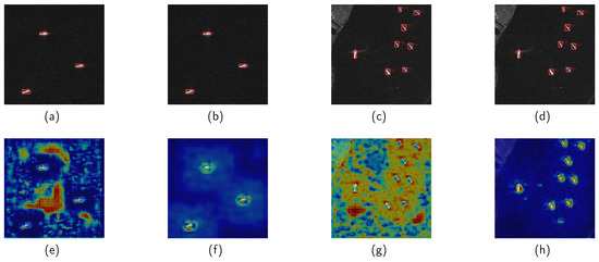
Figure 13.
Comparison of detection results and heatmaps for the baseline (a,c,e,g) and pruned (b,d,f,h) models on the HRSID dataset.
6. Conclusions
This paper proposes a pruning method to ensure a balance in the size and accuracy of remote-sensing target-detection models. The L1RR framework prevents target feature loss during sparse training and pruning. An evaluation of the framework on the NWPU VHR-10 and RSOD datasets demonstrates that the proposed method results in a smaller model size, higher accuracy, and faster detection speed compared to existing lightweight target-detection methods. Moreover, it optimally maintains target features and effectively distinguishes feature channel importance compared to conventional pruning techniques. Importantly, it achieves substantially higher performance than alternate pruning methods for remote-sensing targets with higher detection difficulty. Future studies will investigate the combination of model pruning and model quantization to enhance the efficiency of remote-sensing target detection.
Author Contributions
Conceptualization, Q.R., Y.W. and B.Z.; methodology, M.L. and B.Z.; software, Z.H.; validation, Q.R., Y.W. and B.Z.; formal analysis, M.L. and B.Z.; investigation, Y.W.; resources, Q.R.; data curation, Q.R. and M.L.; writing—original draft preparation, Q.R., Y.W., B.Z. and M.L.; writing—review and editing, Q.R., Y.W. and B.Z.; visualization, Q.R.; supervision, Q.R. and Y.W.; project administration, Y.W.; funding acquisition, Y.W. and B.Z. All authors have read and agreed to the published version of the manuscript.
Funding
This work was supported by the National Key R&D Program of China under Grant 2021YFA0715203.
Data Availability Statement
All data used in this paper are sourced from publicly available data.
Acknowledgments
The author would like to thank the Northwestern Polytechnical University for providing the NWPU VHR-10 data set, as well as Wuhan University for providing the RSOD data set.
Conflicts of Interest
The authors declare no conflicts of interest.
References
- Zhang, B.; Wu, Y.; Zhao, B.; Chanussot, J.; Hong, D.; Yao, J.; Gao, L. Progress and challenges in intelligent remote sensing satellite systems. IEEE J. Sel. Top. Appl. Earth Obs. Remote Sens. 2022, 15, 1814–1822. [Google Scholar] [CrossRef]
- Liu, Z.; Li, J.; Shen, Z.; Huang, G.; Yan, S.; Zhang, C. Learning efficient convolutional networks through network slimming. In Proceedings of the IEEE Conference on Computer Vision and Pattern Recognition (CVPR), Venice, Italy, 22–29 October 2017; pp. 2736–2744. [Google Scholar]
- Ioffe, S.; Szegedy, C. Batch normalization: Accelerating deep network training by reducing internal covariate shift. In Proceedings of the International Conference on Machine Learning (ICML), Lille, France, 6–11 July 2015; pp. 448–456. [Google Scholar]
- Wang, J.; Cui, Z.; Zang, Z.; Meng, X.; Cao, Z. Absorption Pruning of Deep Neural Network for Object Detection in Remote Sensing Imagery. Remote Sens. 2022, 14, 6245. [Google Scholar] [CrossRef]
- Fu, Y.; Zhou, Y.; Yuan, X.; Wei, L.; Bing, H.; Zhang, Y. Efficient Esophageal Lesion Detection using Polarization Regularized Network Slimming. In Proceedings of the 2022 IEEE 8th International Conference on Cloud Computing and Intelligent Systems (CCIS), Chengdu, China, 26–28 November 2022; pp. 46–52. [Google Scholar]
- Xu, Y.; Bai, Y. Compressed YOLOv5 for Oriented Object Detection with Integrated Network Slimming and Knowledge Distillation. In Proceedings of the 2022 3rd International Conference on Information Science, Parallel and Distributed Systems (ISPDS), Guangzhou, China, 22–24 July 2022; pp. 394–403. [Google Scholar]
- He, K.; Zhang, X.; Ren, S.; Sun, J. Deep residual learning for image recognition. In Proceedings of the IEEE Conference on Computer Vision and Pattern Recognition (CVPR), Las Vegas, NV, USA, 27–30 June 2016; pp. 770–778. [Google Scholar]
- Liu, R.; Cao, J.; Li, P.; Sun, W.; Zhang, Y.; Wang, Y. NFP: A No Fine-tuning Pruning Approach for Convolutional Neural Network Compression. In Proceedings of the 2020 3rd International Conference on Artificial Intelligence and Big Data (ICAIBD), Chengdu, China, 28–31 May 2020; pp. 74–77. [Google Scholar]
- Choi, K.; Wi, S.M.; Jung, H.G.; Suhr, J.K. Simplification of Deep Neural Network-Based Object Detector for Real-Time Edge Computing. Sensors 2023, 23, 3777. [Google Scholar] [CrossRef] [PubMed]
- Zhang, P.; Zhong, Y.; Li, X. SlimYOLOv3: Narrower, faster and better for real-time UAV applications. In Proceedings of the IEEE International Conference on Computer Vision Workshops (ICCV), Seoul, Republic of Korea, 27–28 October 2019; pp. 37–45. [Google Scholar]
- Ma, X.; Ji, K.; Xiong, B.; Zhang, L.; Feng, S.; Kuang, G. Light-YOLOv4: An Edge-Device Oriented Target Detection Method for Remote Sensing Images. IEEE J. Sel. Top. Appl. Earth Obs. Remote Sens. 2021, 14, 10808–10820. [Google Scholar] [CrossRef]
- Cheng, G.; Han, J.; Zhou, P.; Guo, L. Multi-class geospatial object detection and geographic image classification based on collection of part detectors. Isprs J. Photogramm. Remote Sens. 2014, 98, 119–132. [Google Scholar] [CrossRef]
- Long, Y.; Gong, Y.; Xiao, Z.; Liu, Q. Accurate object localization in remote sensing images based on convolutional neural networks. IEEE Trans. Geosci. Remote Sens. 2017, 55, 2486–2498. [Google Scholar] [CrossRef]
- Zou, Z.; Shi, Z.; Guo, Y.; Ye, J. Object detection in 20 years: A survey. Proc. IEEE 2023, 111, 257–276. [Google Scholar] [CrossRef]
- Redmon, J.; Divvala, S.; Girshick, R.; Farhadi, A. You only look once: Unified, real-time object detection. In Proceedings of the IEEE Conference on Computer Vision and Pattern Recognition (CVPR), Las Vegas, NV, USA, 27–30 June 2016; pp. 779–788. [Google Scholar]
- Redmon, J.; Farhadi, A. YOLO9000: Better, faster, stronger. In Proceedings of the IEEE Conference on Computer Vision and Pattern Recognition (CVPR), Honolulu, HI, USA, 21–26 July 2017; pp. 7263–7271. [Google Scholar]
- Redmon, J.; Ali, F. Yolov3: An Incremental Improvement. arXiv 2018, arXiv:1804.02767. [Google Scholar]
- Bochkovskiy, A.; Wang, C.Y.; Liao, H.Y.M. YOLOv4: Optimal Speed and Accuracy of Object Detection. arXiv 2020, arXiv:2004.10934. [Google Scholar]
- Glenn, J.; Ayush, C.; Jing, Q. YOLO by Ultralytics. 2021. Available online: https://github.com/ultralytics/yolov5 (accessed on 10 April 2023).
- Ge, Z.; Liu, S.; Wang, F.; Li, Z.; Sun, J. Yolox: Exceeding yolo series in 2021. arXiv 2021, arXiv:2107.08430. [Google Scholar]
- Xu, S.; Wang, X.; Lv, W.; Chang, Q.; Cui, C.; Deng, K.; Wang, G.; Dang, Q.; Wei, S.; Du, Y.; et al. PP-YOLOE: An evolved version of YOLO. arXiv 2022, arXiv:2203.16250. [Google Scholar]
- Wang, C.Y.; Bochkovskiy, A.; Liao, H.Y.M. YOLOv7: Trainable bag-of-freebies sets new state-of-the-art for real-time object detectors. In Proceedings of the IEEE Conference on Computer Vision and Pattern Recognition (CVPR), Vancouver, BC, Canada, 17–24 June 2023; pp. 7464–7475. [Google Scholar]
- Glenn, J.; Ayush, C.; Jing, Q. YOLO by Ultralytics. 2023. Available online: https://github.com/ultralytics/ultralytics (accessed on 15 July 2023).
- Hou, Y.; Shi, G.; Zhao, Y.; Wang, F.; Jiang, X.; Zhuang, R.; Mei, Y.; Ma, X. R-YOLO: A YOLO-Based Method for Arbitrary-Oriented Target Detection in High-Resolution Remote Sensing Images. Sensors 2022, 22, 5716. [Google Scholar] [CrossRef] [PubMed]
- Gong, H.; Mu, T.; Li, Q.; Dai, H.; Li, C.; He, Z.; Wang, W.; Han, F.; Tuniyazi, A.; Li, H.; et al. Swin-Transformer-Enabled YOLOv5 with Attention Mechanism for Small Object Detection on Satellite Images. Remote Sens. 2022, 14, 2861. [Google Scholar] [CrossRef]
- Kim, M.; Jeong, J.; Kim, S. ECAP-YOLO: Efficient Channel Attention Pyramid YOLO for Small Object Detection in Aerial Image. Remote Sens. 2021, 13, 4851. [Google Scholar] [CrossRef]
- Chen, Z.; Liu, C.; Filaretov, V.F.; Yukhimets, D.A. Multi-scale ship detection algorithm based on YOLOv7 for complex scene SAR images. Remote Sens. 2023, 15, 2071. [Google Scholar] [CrossRef]
- He, Y.; Kang, G.; Dong, X.; Fu, Y.; Yang, Y. Soft filter pruning for accelerating deep convolutional neural networks. Sensors 2018, 18, 1–15. [Google Scholar]
- Ye, H.; Zhang, B.; Chen, T.; Fan, J.; Wang, B. Performance-aware approximation of global channel pruning for multitask cnns. IEEE Trans. Pattern Anal. Mach. Intell. 2023, 45, 10267–10284. [Google Scholar] [CrossRef] [PubMed]
- Yang, R.; Chen, Z.; Wang, B.A.; Guo, Y.; Hu, L. A Lightweight Detection Method for Remote Sensing Images and Its Energy-Efficient Accelerator on Edge Devices. Sensors 2023, 23, 6497. [Google Scholar] [CrossRef]
- Xu, X.; Zhang, X.; Zhang, T. Lite-YOLOv5: A Lightweight Deep Learning Detector for On-Board Ship Detection in Large-Scene Sentinel-1 SAR Images. Remote Sens. 2022, 14, 1018. [Google Scholar] [CrossRef]
- Candes, E.J.; Wakin, M.B.; Boyd, S.P. Enhancing sparsity by reweighted L1 minimization. J. Fourier Anal. Appl. 2008, 14, 877–905. [Google Scholar] [CrossRef]
- Liu, W.; Anguelov, D.; Erhan, D.; Szegedy, C.; Reed, S.; Fu, C.Y.; Berg, A.C. SSD: Single Shot Multibox Detector. In Proceedings of the 14th European Conference on Computer Vision(ECCV), Amsterdam, The Netherlands, 11–14 October 2016; Volume 14, pp. 21–37. [Google Scholar]
- Chen, X.; Gong, Z. YOLOv5-Lite: Lighter, Faster, and Easier to Deploy. 2021. Available online: https://github.com/ppogg/YOLOv5-Lite (accessed on 10 June 2023).
- RangiLyu. Nanodet-Plus: Super Fast and Lightweight Anchor-Free Object Detection Model. 2021. Available online: https://github.com/RangiLyu/nanodet (accessed on 10 June 2023).
- Yi, H.; Liu, B.; Zhao, B.; Liu, E. Small Object Detection Algorithm Based on Improved YOLOv8 for Remote Sensing. IEEE J. Sel. Top. Appl. Earth Obs. Remote Sens. 2024, 17, 1734–1747. [Google Scholar] [CrossRef]
- Ren, S.; He, K.; Girshick, R.; Sun, J. Faster r-cnn: Towards real-time object detection with region proposal networks. In Proceedings of the Advances in Neural Information Processing Systems 2015 (NIPS), Montreal, QC, Canada, 7–12 December 2015; Volume 28. [Google Scholar]
- Shi, L.; Kuang, L.; Xu, X.; Pan, B.; Shi, Z. CANet: Centerness-aware network for object detection in remote sensing images. IEEE Trans. Geosci. Remote Sens. 2022, 60, 1–13. [Google Scholar] [CrossRef]
- Li, Z.; Wang, Y.; Zhang, Y.; Gao, Y.; Zhao, Z.; Feng, H.; Zhao, T. Context Feature Integration and Balanced Sampling Strategy for Small Weak Object Detection in Remote-Sensing Imagery. IEEE Geosci. Remote Sens. Lett. 2024, 21, 1. [Google Scholar] [CrossRef]
- Chattopadhay, A.; Sarkar, A.; Howlader, P.; Balasubramanian, V.N. Grad-CAM++: Generalized gradient-based visual explanations for deep convolutional networks. In Proceedings of the 2018 IEEE Winter Conference on Applications of Computer Vision (WACV), Lake, Tahoe, NV, USA, 12–15 March 2018; pp. 839–847. [Google Scholar]
- Xie, T.; Han, W.; Xu, S. OYOLO: An Optimized YOLO Method for Complex Objects in Remote Sensing Image Detection. IEEE Geosci. Remote Sens. Lett. 2023, 1. [Google Scholar] [CrossRef]
- Kang, H.; Liu, Y. Efficient Object Detection with Deformable Convolution for Optical Remote Sensing Imagery. In Proceedings of the 2022 5th International Conference on Pattern Recognition and Artificial Intelligence (PRAI), Chengdu, China, 19–21 August 2022; pp. 1108–1114. [Google Scholar]
- Wei, S.; Zeng, X.; Qu, Q.; Wang, M.; Su, H.; Shi, J. HRSID: A high-resolution SAR images dataset for ship detection and instance segmentation. IEEE Access 2020, 8, 120234–120254. [Google Scholar] [CrossRef]
- Gao, S.; Liu, J.; Miao, Y.; He, Z. A high-effective implementation of ship detector for SAR images. IEEE Geosci. Remote Sens. Lett. 2021, 19, 1–5. [Google Scholar] [CrossRef]
- Wei, H.; Wang, Z.; Hua, G.; Ni, Y. A Zero-Shot NAS Method for SAR Ship Detection Under Polynomial Search Complexity. IEEE Signal Process. Lett. 2024, 31, 1329–1333. [Google Scholar] [CrossRef]


Disclaimer/Publisher’s Note: The statements, opinions and data contained in all publications are solely those of the individual author(s) and contributor(s) and not of MDPI and/or the editor(s). MDPI and/or the editor(s) disclaim responsibility for any injury to people or property resulting from any ideas, methods, instructions or products referred to in the content. |
© 2024 by the authors. Licensee MDPI, Basel, Switzerland. This article is an open access article distributed under the terms and conditions of the Creative Commons Attribution (CC BY) license (https://creativecommons.org/licenses/by/4.0/).