
Using the Improved YOLOv5-Seg Network and Sentinel-2 Imagery to Map Glacial Lakes in High Mountain Asia

 , , , ,
Abstract
1. Introduction
2. Materials and Methods
2.1. Data Sources
2.2. Methods
2.2.1. Data Preprocessing
2.2.2. Improved Convolutional Neural Network
- (1)
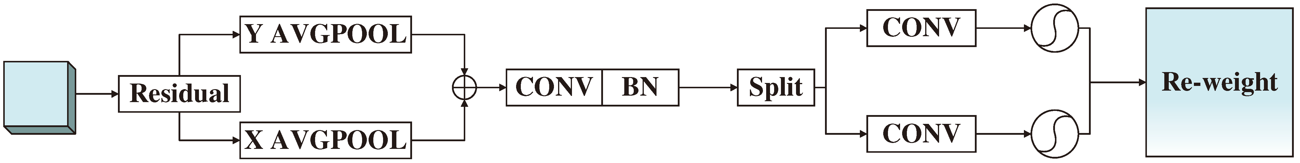
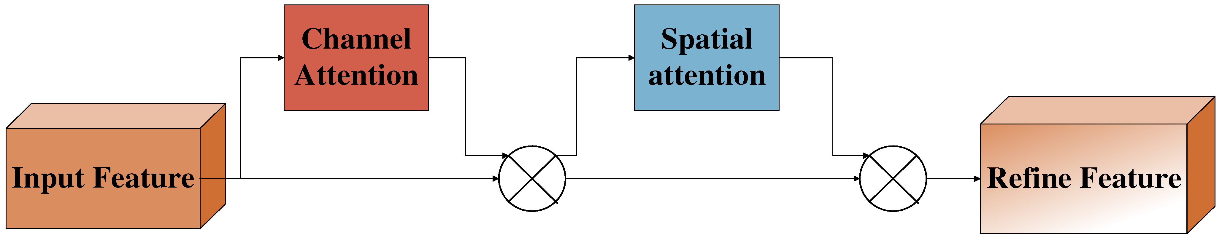
- Attention mechanism
- (2)
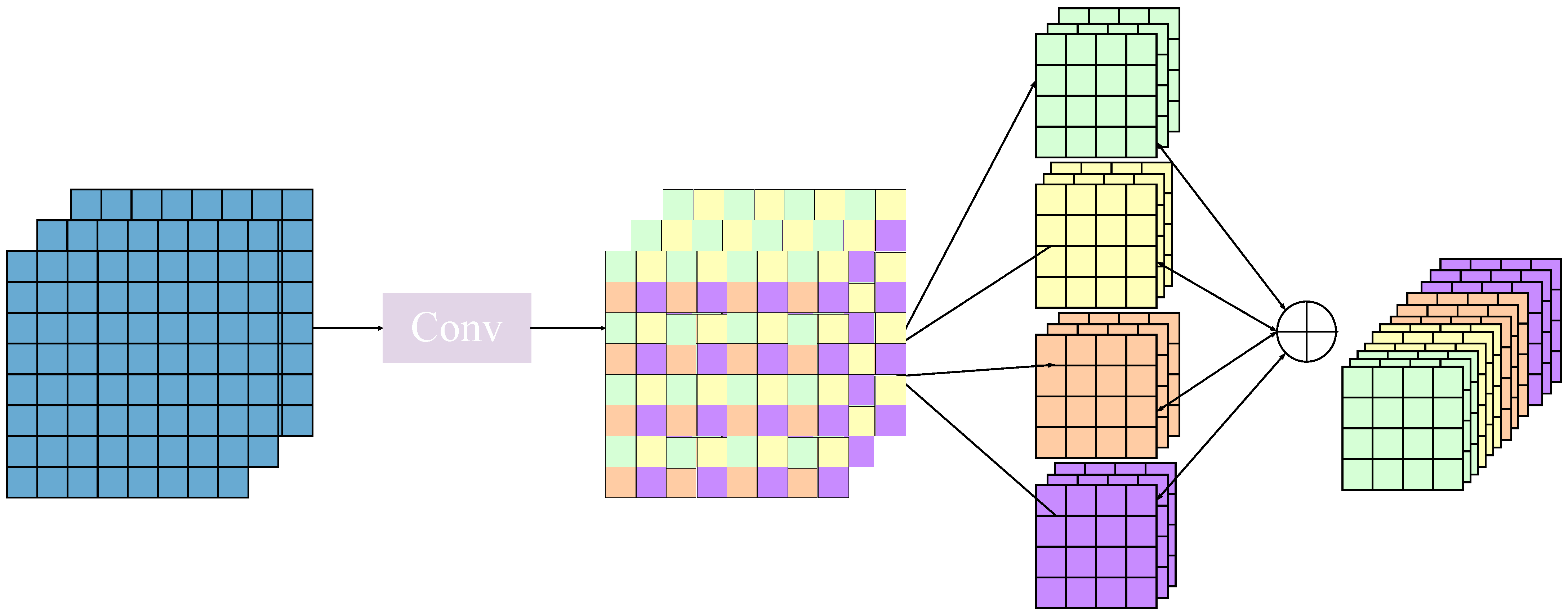
- Space-to-depth (SPD) module
- (3)
- Small target layers
2.2.3. Postprocessing and Accuracy Assessment
3. Results
3.1. Performance of the Proposed Method
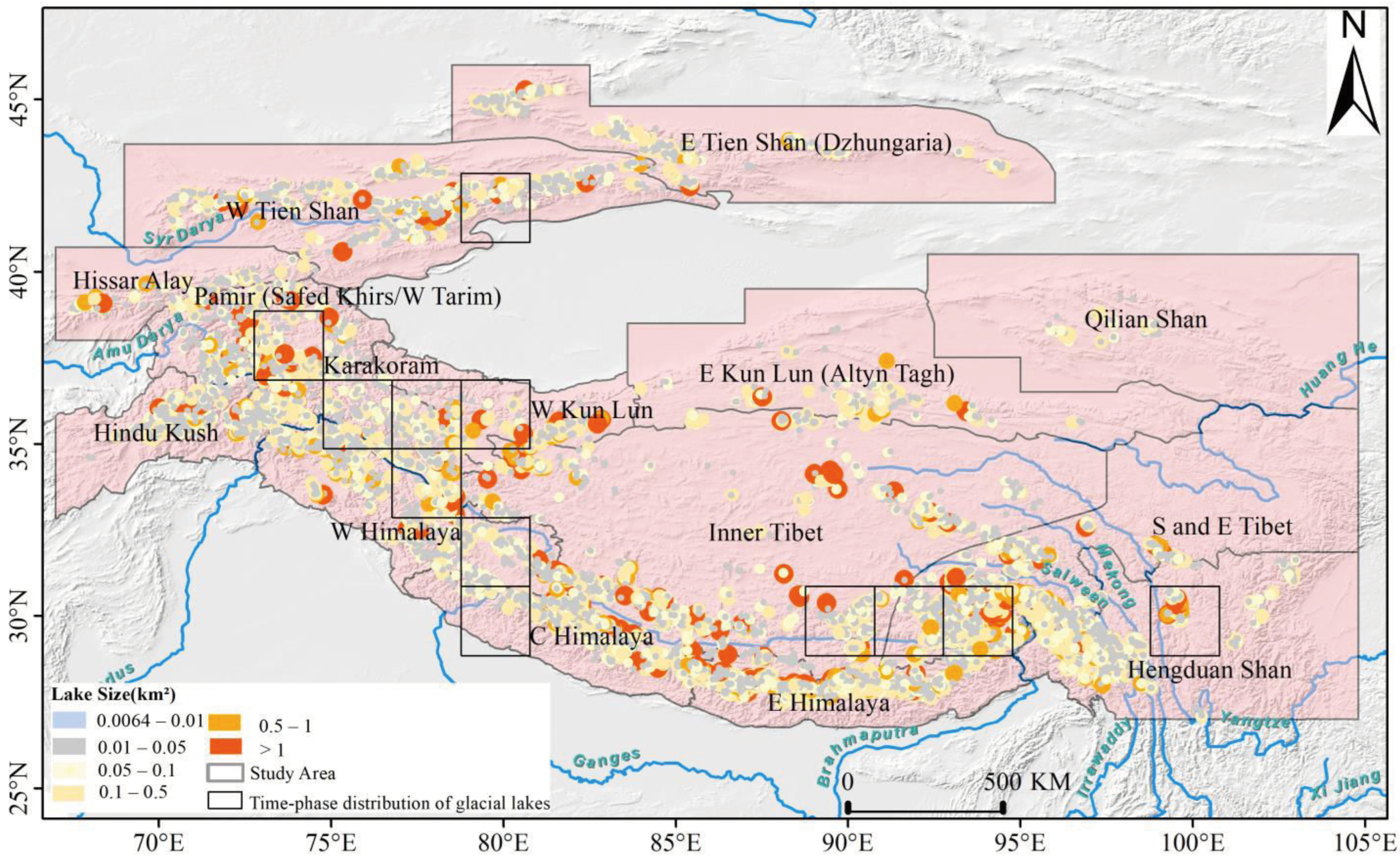
3.2. Mapping of Glacial Lakes in HMA
4. Discussion
4.1. Advantages of the Improved Strategies
4.2. Reliability of the Present Glacial Lake Inventory
5. Conclusions
Author Contributions
Funding
Data Availability Statement
Acknowledgments
Conflicts of Interest
References
- Qin, D.; Yao, T.; Ding, Y. Glossary of Cryosphere Science, 2nd ed.; China Meteorological Press: Beijing, China, 2014. [Google Scholar]
- Wang, X.; Guo, X.; Yang, C.; Liu, Q.; Wei, J.; Zhang, Y.; Liu, S.; Zhang, Y.; Jiang, Z.; Tang, Z. Glacial lake inventory of high-mountain Asia in 1990 and 2018 derived from Landsat images. Earth Syst. Sci. Data 2020, 12, 2169–2182. [Google Scholar] [CrossRef]
- Guillet, G.; King, O.; Lv, M.; Ghuffar, S.; Benn, D.; Quincey, D.; Bolch, T. A regionally resolved inventory of High Mountain Asia surge-type glaciers, derived from a multi-factor remote sensing approach. Cryosphere 2022, 16, 603–623. [Google Scholar] [CrossRef]
- Wang, X.; Ran, W.; Wei, J.; Yin, Y.; Liu, S.; Bolch, T.; Zhang, Y.; Xue, X.; Ding, Y.; Liu, Q.; et al. Spatially resolved glacial meltwater retainment in glacial lakes exerts increasing impacts in High Mountain Asia. J. Hydrol. 2024, 633, 130967. [Google Scholar] [CrossRef]
- Bhattacharya, A.; Bolch, T.; Mukherjee, K.; King, O.; Menounos, B.; Kapitsa, V.; Neckel, N.; Yang, W.; Yao, T. High Mountain Asian glacier response to climate revealed by multi-temporal satellite observations since the 1960s. Nat. Commun. 2021, 12, 4133. [Google Scholar] [CrossRef]
- Yao, T.; Bolch, T.; Chen, D.; Gao, J.; Immerzeel, W.; Piao, S.; Su, F.; Thompson, L.; Wada, Y.; Wang, L.; et al. The imbalance of the Asian water tower. Nat. Rev. Earth Environ. 2022, 3, 618–632. [Google Scholar] [CrossRef]
- Nie, Y.; Liu, Q.; Wang, J.; Zhang, Y.; Sheng, Y.; Liu, S. An inventory of historical glacial lake outburst floods in the Himalayas based on remote sensing observations and geomorphological analysis. Geomorphology 2018, 308, 91–106. [Google Scholar] [CrossRef]
- Shugar, D.H.; Burr, A.; Haritashya, U.K.; Kargel, J.S.; Watson, C.S.; Kennedy, M.C.; Bevington, A.R.; Betts, R.A.; Harrison, S.; Strattman, K. Rapid worldwide growth of glacial lakes since 1990. Nat. Clim. Chang. 2020, 10, 939–945. [Google Scholar] [CrossRef]
- Shrestha, F.; Steiner, J.F.; Shrestha, R.; Dhungel, Y.; Joshi, S.P.; Inglis, S.; Ashraf, A.; Wali, S.; Walizada, K.M.; Zhang, T. HMAGLOFDB v1. 0–a comprehensive and version controlled database of glacier lake outburst floods in high mountain Asia. Earth Syst. Sci. Data Discuss. 2023, 15, 3941–3961. [Google Scholar] [CrossRef]
- Chen, F.; Zhang, M.; Guo, H.; Allen, S.; Kargel, J.S.; Haritashya, U.K.; Watson, C.S. Annual 30 m dataset for glacial lakes in High Mountain Asia from 2008 to 2017. Earth Syst. Sci. Data 2021, 13, 741–766. [Google Scholar] [CrossRef]
- Rounce, D.R.; Hock, R.; Maussion, F.; Hugonnet, R.; Kochtitzky, W.; Huss, M.; Berthier, E.; Brinkerhoff, D.; Compagno, L.; Copland, L.; et al. Global glacier change in the 21st century: Every increase in temperature matters. Science 2023, 379, 78–83. [Google Scholar] [CrossRef] [PubMed]
- Zhao, F.; Long, D.; Li, X.; Huang, Q.; Han, P. Rapid glacier mass loss in the Southeastern Tibetan Plateau since the year 2000 from satellite observations. Remote Sens. Environ. 2022, 270, 112853. [Google Scholar] [CrossRef]
- Nie, Y.; Deng, Q.; Pritchard, H.D.; Carrivick, J.L.; Ahmed, F.; Huggel, C.; Liu, L.; Wang, W.; Lesi, M.; Wang, J. Glacial lake outburst floods threaten Asia’s infrastructure. Sci. Bull. 2023, 68, 1361–1365. [Google Scholar] [CrossRef]
- Wangchuk, S.; Bolch, T. Mapping of glacial lakes using Sentinel-1 and Sentinel-2 data and a random forest classifier: Strengths and challenges. Sci. Remote Sens. 2020, 2, 100008. [Google Scholar] [CrossRef]
- Lesi, M.; Nie, Y.; Shugar, D.H.; Wang, J.; Deng, Q.; Chen, H.; Fan, J. Landsat- and Sentinel-derived glacial lake dataset in the China–Pakistan Economic Corridor from 1990 to 2020. Earth Syst. Sci. Data 2022, 14, 5489–5512. [Google Scholar] [CrossRef]
- Wang, S.; Peppa, M.V.; Xiao, W.; Maharjan, S.B.; Joshi, S.P.; Mills, J.P. A second-order attention network for glacial lake segmentation from remotely sensed imagery. ISPRS J. Photogramm. Remote Sens. 2022, 189, 289–301. [Google Scholar] [CrossRef]
- Gao, B.-c. NDWI—A normalized difference water index for remote sensing of vegetation liquid water from space. Remote Sens. Environ. 1996, 58, 257–266. [Google Scholar] [CrossRef]
- Salomonson, V.V.; Appel, I. Estimating fractional snow cover from MODIS using the normalized difference snow index. Remote Sens. Environ. 2004, 89, 351–360. [Google Scholar] [CrossRef]
- Xu, H. A study on information extraction of water body with the modified normalized difference water index (MNDWI). J. Remote Sens. 2005, 9, 595. [Google Scholar]
- Wang, J.; Chen, F.; Zhang, M.; Yu, B. NAU-Net: A New Deep Learning Framework in Glacial Lake Detection. IEEE Geosci. Remote Sens. Lett. 2022, 19, 2000905. [Google Scholar] [CrossRef]
- Dirscherl, M.; Dietz, A.J.; Kneisel, C.; Kuenzer, C. Automated mapping of Antarctic supraglacial lakes using a machine learning approach. Remote Sens. 2020, 12, 1203. [Google Scholar] [CrossRef]
- Thati, J.; Ari, S. A systematic extraction of glacial lakes for satellite imagery using deep learning based technique. Measurement 2022, 192, 110858. [Google Scholar] [CrossRef]
- Wu, R.; Liu, G.; Zhang, R.; Wang, X.; Li, Y.; Zhang, B.; Cai, J.; Xiang, W. A Deep Learning Method for Mapping Glacial Lakes from the Combined Use of Synthetic-Aperture Radar and Optical Satellite Images. Remote Sens. 2020, 12, 4020. [Google Scholar] [CrossRef]
- Jiang, D.; Li, X.; Zhang, K.; Marinsek, S.; Hong, W.; Wu, Y. Automatic Supraglacial Lake Extraction in Greenland Using Sentinel-1 SAR Images and Attention-Based U-Net. Remote Sens. 2022, 14, 4998. [Google Scholar] [CrossRef]
- Cao, Y.; Bai, X.; Pan, M.; Lei, R.; Du, P. Refined glacial lake extraction in high Asia region by Deep Neural Network and Superpixel-based Conditional Random Field. Cryosphere Discuss. 2023, 2023, 1–21. [Google Scholar] [CrossRef]
- Dirscherl, M.; Dietz, A.J.; Kneisel, C.; Kuenzer, C. A Novel Method for Automated Supraglacial Lake Mapping in Antarctica Using Sentinel-1 SAR Imagery and Deep Learning. Remote Sens. 2021, 13, 197. [Google Scholar] [CrossRef]
- Qayyum, N.; Ghuffar, S.; Ahmad, H.M.; Yousaf, A.; Shahid, I. Glacial lakes mapping using multi satellite PlanetScope imagery and deep learning. ISPRS Int. J. Geo-Inf. 2020, 9, 560. [Google Scholar] [CrossRef]
- Kaushik, S.; Singh, T.; Joshi, P.K.; Dietz, A.J. Automated mapping of glacial lakes using multisource remote sensing data and deep convolutional neural network. Int. J. Appl. Earth Obs. Geoinf. 2022, 115, 103085. [Google Scholar] [CrossRef]
- Guo, W.; Liu, S.; Xu, J.; Wu, L.; Shangguan, D.; Yao, X.; Wei, J.; Bao, W.; Yu, P.; Liu, Q.; et al. The second Chinese glacier inventory: Data, methods and results. J. Glaciol. 2015, 61, 357–372. [Google Scholar] [CrossRef]
- Pfeffer, W.T.; Arendt, A.A.; Bliss, A.; Bolch, T.; Cogley, J.G.; Gardner, A.S.; Hagen, J.-O.; Hock, R.; Kaser, G.; Kienholz, C.; et al. The Randolph Glacier Inventory: A globally complete inventory of glaciers. J. Glaciol. 2014, 60, 537–552. [Google Scholar] [CrossRef]
- Hou, Q.; Zhou, D.; Feng, J. Coordinate attention for efficient mobile network design. In Proceedings of the IEEE/CVF Conference on Computer Vision and Pattern Recognition, Nashville, TN, USA, 19–25 June 2021; pp. 13713–13722. [Google Scholar]
- Woo, S.; Park, J.; Lee, J.-Y.; Kweon, I.S. Cbam: Convolutional block attention module. In Proceedings of the European Conference on Computer Vision (ECCV), Munich, Germany, 8–14 September 2018; pp. 3–19. [Google Scholar]
- Zhu, X.; Lyu, S.; Wang, X.; Zhao, Q. TPH-YOLOv5: Improved YOLOv5 based on transformer prediction head for object detection on drone-captured scenarios. In Proceedings of the IEEE/CVF International Conference on Computer Vision, Montreal, BC, Canada, 10–17 October 2021; pp. 2778–2788. [Google Scholar]
- Sunkara, R.; Luo, T. No More Strided Convolutions or Pooling: A New CNN Building Block for Low-Resolution Images and Small Objects. In Proceedings of the Machine Learning and Knowledge Discovery in Databases, Turin, Italy, 18–22 September 2023; Springer: Cham, Switzerland, 2023; pp. 443–459. [Google Scholar]
- Wan, D.; Lu, R.; Wang, S.; Shen, S.; Xu, T.; Lang, X. YOLO-HR: Improved YOLOv5 for Object Detection in High-Resolution Optical Remote Sensing Images. Remote Sens. 2023, 15, 614. [Google Scholar] [CrossRef]
- Bian, L.; Li, B.; Wang, J.; Gao, Z. Multi-branch stacking remote sensing image target detection based on YOLOv5. Egypt. J. Remote Sens. Space Sci. 2023, 26, 999–1008. [Google Scholar] [CrossRef]
- Li, J.; Sheng, Y. An automated scheme for glacial lake dynamics mapping using Landsat imagery and digital elevation models: A case study in the Himalayas. Int. J. Remote Sens. 2012, 33, 5194–5213. [Google Scholar] [CrossRef]
- Wang, C.-Y.; Yeh, I.-H.; Liao, H.-Y.M. You only learn one representation: Unified network for multiple tasks. arXiv 2021, arXiv:2105.04206. [Google Scholar]
- Wang, C.-Y.; Bochkovskiy, A.; Liao, H.-Y.M. YOLOv7: Trainable bag-of-freebies sets new state-of-the-art for real-time object detectors. In Proceedings of the IEEE/CVF Conference on Computer Vision and Pattern Recognition, Vancouver, BC, Canada, 17–24 June 2023; pp. 7464–7475. [Google Scholar]
- Ronneberger, O.; Fischer, P.; Brox, T. U-Net: Convolutional Networks for Biomedical Image Segmentation. In Proceedings of the Medical Image Computing and Computer-Assisted Intervention—MICCAI 2015, Munich, Germany, 5–9 October 2015; Springer: Cham, Switzerland, 2015; pp. 234–241. [Google Scholar]
- Badrinarayanan, V.; Kendall, A.; Cipolla, R. SegNet: A Deep Convolutional Encoder-Decoder Architecture for Image Segmentation. IEEE Trans. Pattern Anal. Mach. Intell. 2017, 39, 2481–2495. [Google Scholar] [CrossRef] [PubMed]
- Dou, X.; Fan, X.; Wang, X.; Yunus, A.P.; Xiong, J.; Tang, R.; Lovati, M.; van Westen, C.; Xu, Q. Spatio-Temporal Evolution of Glacial Lakes in the Tibetan Plateau over the Past 30 Years. Remote Sens. 2023, 15, 416. [Google Scholar] [CrossRef]
- Abe, C.; Fujita, K.; Kawamoto, S.; Narama, C.; Nishimura, K.; Tadono, T.; Tomiyama, N.; Uda, T.; Ukita, J.; Yabuki, H.; et al. Glacial lake inventory of Bhutan using ALOS data: Methods and preliminary results. Ann. Glaciol. 2011, 52, 65–71. [Google Scholar] [CrossRef]
- Xu, J.; Feng, M.; Sui, Y.; Yan, D.; Zhang, K.; Shi, K. Identifying Alpine Lakes in the Eastern Himalayas Using Deep Learning. Water 2023, 15, 229. [Google Scholar] [CrossRef]
- Zhang, M.; Chen, F.; Guo, H.; Yi, L.; Zeng, J.; Li, B. Glacial Lake Area Changes in High Mountain Asia during 1990–2020 Using Satellite Remote Sensing. Research 2022, 2022, 9821275. [Google Scholar] [CrossRef]
- Yin, Y.; Wang, X.; Liu, S.; Guo, X.; Zhang, Y.; Ran, W.; Wang, Q. Variation characteristics and influencing factors of glacial lakes in China from 1990 to 2020. Lake Sci. 2023, 35, 358–367. [Google Scholar]
- Zhang, M.; Chen, F.; Zhao, H.; Wang, J.; Wang, N. Recent Changes of Glacial Lakes in the High Mountain Asia and Its Potential Controlling Factors Analysis. Remote Sens. 2021, 13, 3757. [Google Scholar] [CrossRef]


| Algorithm | Precision | Recall | mAP_0.5 | F1 Score | Bands |
|---|---|---|---|---|---|
| YOLOv5-seg | 0.6 | 0.64 | 0.56 | 0.62 | 8 4 3 |
| YOLOv7-seg | 0.651 | 0.71 | 0.78 | 0.70 | 8 4 3 |
| YOLOR-seg | 0.583 | 0.731 | 0.60 | 0.790 | 8 4 3 |
| YOLOv8-seg | 0.916 | 0.75 | 0.77 | 0.82 | 8 4 3 |
| Improved YOLOv5-seg | 0.702 | 0.711 | 0.75 | 0.71 | 4 3 2 |
| YOLOv5-seg | 0.673 | 0.701 | 0.724 | 0.687 | 4 3 2 |
| Improved YOLOv5-seg(CA) | 0.87 | 0.801 | 0.88 | 0.84 | 8 4 3 |
| Improved YOLOv5-seg(CBAM) | 0.95 | 0.928 | 0.96 | 0.94 | 8 4 3 |
| Improved YOLOv5-seg(CA) | 0.916 | 0.734 | 0.80 | 0.81 | 11 4 3 |
| Index | CA | CBAM | Small-Object Detection Layer | SPD-Conv | C2f | mAP_0.5 | F1 Score |
|---|---|---|---|---|---|---|---|
| YOLOv5-seg | - | - | - | - | - | 0.56 | 0.62 |
| 1 | √ | - | - | - | - | 0.62 | 0.65 |
| 2 | √ | - | √ | - | - | 0.73 | 0.70 |
| YOLOv8-seg | - | - | - | - | √ | 0.77 | 0.82 |
| 4 | √ | - | - | - | √ | 0.88 | 0.84 |
| 5 | - | √ | - | - | √ | 0.88 | 0.85 |
| 6 | √ | - | - | √ | √ | 0.87 | 0.83 |
| Improved YOLOv5-seg (CBAM) | - | √ | - | √ | √ | 0.96 | 0.94 |
| Algorithm | Recall | Precision | Saccuracy | F1 Score | Bands |
|---|---|---|---|---|---|
| Improved YOLOv5-seg | 0.70 | 0.80 | 0.95 | 0.75 | (4,3,2) |
| Improved YOLOv5-seg (CA) | 0.76 | 0.86 | 0.95 | 0.81 | (8,4,3) |
| Improved YOLOv5-seg (CA) | 0.81 | 0.84 | 0.94 | 0.82 | (11,4,3) |
| Improved YOLOv5-seg (CBAM) | 0.82 | 0.89 | 0.92 | 0.85 | (8,4,3) |
| Combined the improved algorithms | 0.87 | 0.89 | 0.96 | 0.89 | (11,8,4,3,2) |
Disclaimer/Publisher’s Note: The statements, opinions and data contained in all publications are solely those of the individual author(s) and contributor(s) and not of MDPI and/or the editor(s). MDPI and/or the editor(s) disclaim responsibility for any injury to people or property resulting from any ideas, methods, instructions or products referred to in the content. |
© 2024 by the authors. Licensee MDPI, Basel, Switzerland. This article is an open access article distributed under the terms and conditions of the Creative Commons Attribution (CC BY) license (https://creativecommons.org/licenses/by/4.0/).
Share and Cite
Yin, L.; Wang, X.; Du, W.; Yang, C.; Wei, J.; Wang, Q.; Lei, D.; Xiao, J. Using the Improved YOLOv5-Seg Network and Sentinel-2 Imagery to Map Glacial Lakes in High Mountain Asia. Remote Sens. 2024, 16, 2057. https://doi.org/10.3390/rs16122057
Yin L, Wang X, Du W, Yang C, Wei J, Wang Q, Lei D, Xiao J. Using the Improved YOLOv5-Seg Network and Sentinel-2 Imagery to Map Glacial Lakes in High Mountain Asia. Remote Sensing. 2024; 16(12):2057. https://doi.org/10.3390/rs16122057
Chicago/Turabian StyleYin, Lichen, Xin Wang, Wentao Du, Chengde Yang, Junfeng Wei, Qiong Wang, Dongyu Lei, and Jingtao Xiao. 2024. "Using the Improved YOLOv5-Seg Network and Sentinel-2 Imagery to Map Glacial Lakes in High Mountain Asia" Remote Sensing 16, no. 12: 2057. https://doi.org/10.3390/rs16122057
APA StyleYin, L., Wang, X., Du, W., Yang, C., Wei, J., Wang, Q., Lei, D., & Xiao, J. (2024). Using the Improved YOLOv5-Seg Network and Sentinel-2 Imagery to Map Glacial Lakes in High Mountain Asia. Remote Sensing, 16(12), 2057. https://doi.org/10.3390/rs16122057