Abstract
Glacier inventories are fundamental in understanding glacier dynamics and glacier-related environmental processes. High-resolution mapping of glacier outlines is lacking, although high-resolution satellite images have become available in recent decades. Challenges in development of glacier inventories have always included accurate delineation of boundaries of debris-covered glaciers, which is particularly true for high-resolution satellite images due to their limited spectral bands. To address this issue, we introduced an automated, high-precision method in this study for mapping debris-covered glaciers based on 1 m resolution Gaofen-2 (GF-2) imagery. By integrating GF-2 reflectance, topographic features, and land surface temperature (LST), we used an attention mechanism to improve the performance of several deep learning network models (the U-Net network, a fully convolutional neural network (FCNN), and DeepLabV3+). The trained models were then applied to map the outlines of debris-covered glaciers, at 1 m resolution, in the central Karakoram regions. The results indicated that the U-Net model enhanced with the Convolutional Block Attention Module (CBAM) outperforms other deep learning models (e.g., FCNN, DeepLabV3+, and U-Net model without CBAM) in terms of precision for supraglacial debris identification. On the testing dataset, the CBAM-enhanced U-Net model achieved notable performance metrics, with its accuracy, F1 score, mean intersection over union (MIoU), and kappa coefficient reaching 0.93, 0.74, 0.79, and 0.88. When applied at the regional scale, the model even exhibits heightened precision (accuracies = 0.94, F1 = 0.94, MIoU = 0.86, kappa = 0.91) in mapping debris-covered glaciers. The experimental glacier outlines were accurately extracted, enabling the distinction of supraglacial debris, clean ice, and other features on glaciers in central Karakoram using this trained model. The results for our method revealed differences of 0.14% for bare ice and 10.36% against the manually interpreted glacier boundary for supraglacial debris. Comparison with previous glacier inventories revealed raised precisions of 8.74% and 4.78% in extracting clean ice and with supraglacial debris, respectively. Additionally, our model demonstrates exceptionally high exclusion for bare rock outside glaciers and could reduce the influence of non-glacial snow on glacier delineation, showing substantial promise in mapping debris-covered glaciers.
1. Introduction
Glaciers exert considerable influence on the allocation of water resources, hydrological fluctuations, ecological stability, and socioeconomic development [1,2,3]. The retreat of glaciers in High Mountain Asia (HMA), driven by climate change and intensifying global warming, has become a significant concern. This accelerated melt poses significant threats to regional water security, increasing the likelihood of mountain-related hazards such as floods, debris flows, and other glacier-associated disasters, while also contributing to rising sea levels [4,5,6,7,8,9]. An accurate and reliable glacier inventory serves as the foundation for examining accuracy in projecting glacier changes, underscoring the importance of precisely delineating glacier boundaries. However, debris-covered glaciers add layers of complexity to glacier outline extraction. Supraglacial debris includes materials from glacier abrasion or excavation processes. It also comprises rock debris and sediment surrounding glaciers, resulting from solifluction, ice/snow/rock avalanches, and gravitational sliding, which cause rock fragments to collapse onto the glacier surface [10,11,12]. Debris-covered glaciers are prevalent in the HMA regions, including the TianShan Mountains, Pamir, Karakoram, the Himalayas, and the southeastern Tibetan plateau [13,14,15]. A considerable portion (~10%) of glaciers in the Karakoram is covered by debris [16,17]. The supraglacial debris mainly concentrates within the ablation zone of glaciers, exhibiting similar spectral characteristics to the surrounding rock environment in remote sensing imagery, posing challenges for distinguishing them from each other [18,19]. The use of automated techniques to map debris-covered glaciers will improve the mapping process by reducing the impact of manual visual interpretation and the subjective factors that arise [18,20].
Various methods, including threshold segmentation methods, object-based classification, synthetic aperture radar interferometry, and machine learning approaches, have been used for clean ice/snow and supraglacial debris mapping [21,22,23,24,25]. These approaches exhibit commendable precision in clean ice and snow extraction; nevertheless, challenges still persist in the extraction of supraglacial debris. Fortunately, deep learning techniques have demonstrated significant potential in the area of supraglacial debris extraction. Numerous studies have been conducted to automatically delineate glacier boundaries and supraglacial debris boundaries by employing various deep neural networks and multisource remote sensing data [26,27,28,29,30], which demonstrate the robust automated processing and advanced feature extraction capabilities of deep learning [31,32]. The deep learning models used for glacier extraction predominantly encompass the U-Net [33] and DeepLabV3+ models [34]. These models have been effectively employed in the delineation of marine ice margins [35], as well as in demarcating rock glacier boundaries and mapping debris-covered glaciers [28,36,37].
However, the accurate extraction of glacial and supraglacial debris using medium- to low-resolution images is difficult, particularly in terms of identifying changing glacier boundaries or smaller areas, which presents limitations in the extraction of small glaciers [38]. Previous studies indicate that leveraging fine features on high-resolution imagery can significantly enhance the accuracy of glacier outline extraction [38,39,40]. Nevertheless, the lack of shortwave infrared and thermal infrared bands in high-resolution images limits the calculation of the Normalized Difference Snow Index (NDSI) and diminishes the efficacy of band combinations, impeding conventional techniques for extracting supraglacial debris. Additionally, unlike bare ice extraction, the identification of supraglacial debris often requires the integration of multiple features, including thermal infrared radiation, topographic factors, and SAR, among others [18,28,41,42,43]. High-resolution imagery provides spectral features, such as shape and texture, which are essential for distinguishing supraglacial debris [44,45,46], and DEMs are useful in glacier extraction due to the significant elevation difference between glacier and non-glacier areas [18,47]; there are notable temperature differences between glacier and non-glacier regions: the glacier temperatures are typically lower in comparison to those of supraglacial debris [19,41]. These temperature variations can be attributed to differences in reflectivity. To sum up, given the increasing availability of publicly accessible high-resolution images for both civilian and commercial purposes, the development of an efficient method for automatically delineating supraglacial debris based on fine features holds substantial practical value. The incorporation of diverse datasets [19,29,48,49], combined with the advanced feature extraction capabilities of deep learning, presents significant potential for the automated and precise extraction of debris-covered glaciers. This fusion represents a robust and effective technological approach for such endeavors.
This study aims to present an automated approach for the extraction of supraglacial debris. We employed an attention-mechanism-optimized deep learning semantic segmentation model (U-Net and DeepLabV3+) to automatically extract supraglacial debris and glacier outlines based on spectral features derived from GF-2 imagery, topographic features, and LST. To evaluate the efficacy and reliability of our methodology, a specific area within the Karakoram Mountains was selected for testing. The accuracy of the proposed approach is assessed by comparing the experimental results with manually delineated glacier outlines based on GF-2 imagery. The Karakoram glacier inventories (KGIs) [17] are employed as a reference to compare the results for accuracy assessment. This paper is subdivided into five sections. Section 1 presents an overview of the current state of the research. Section 2 provides a detailed description of the data and methodology employed in this study. Section 3 presents the principal results of the study. Section 4 describes the discussion of the research findings. The overall results are concluded in Section 5.
2. Data and Methods
2.1. Study Area
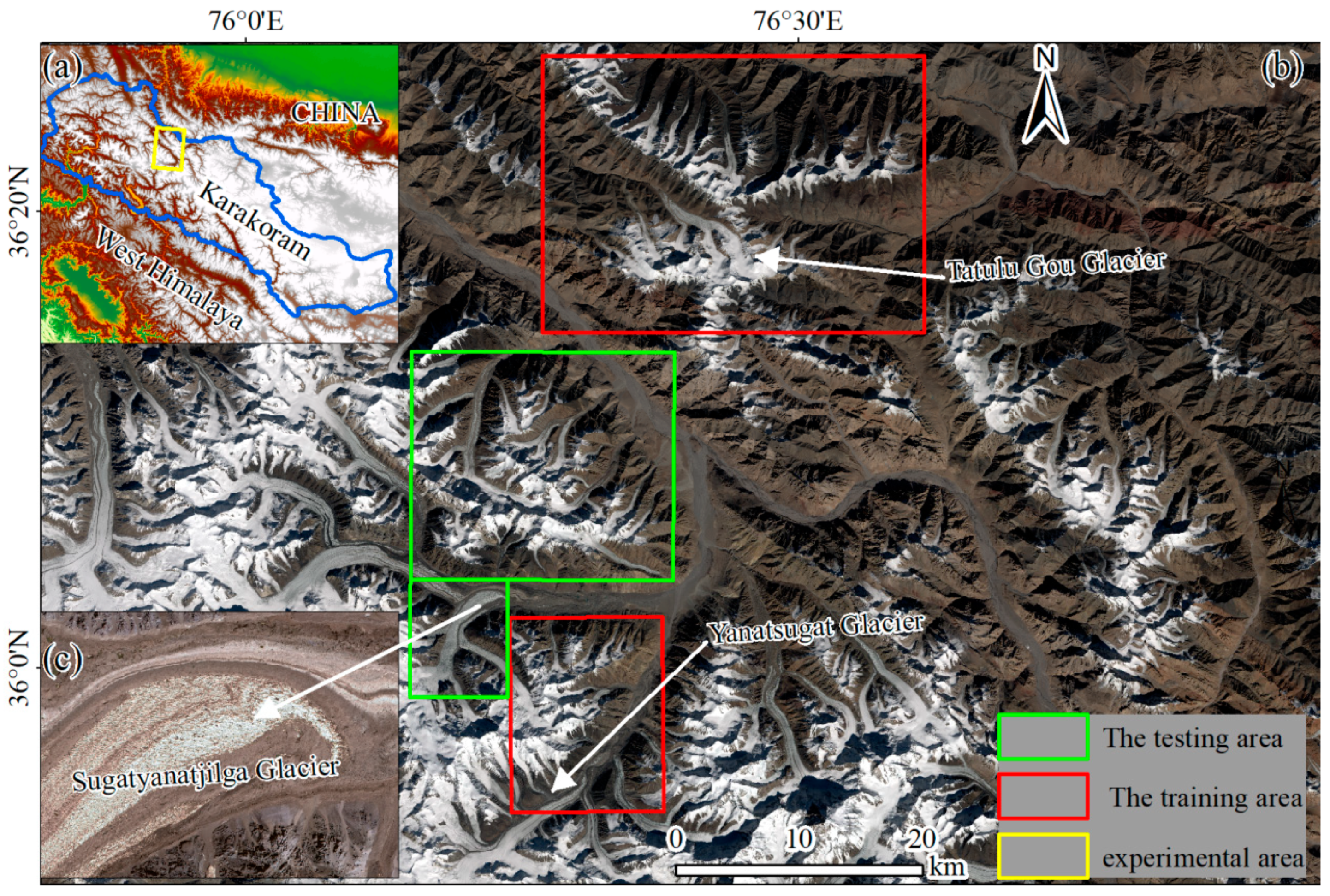
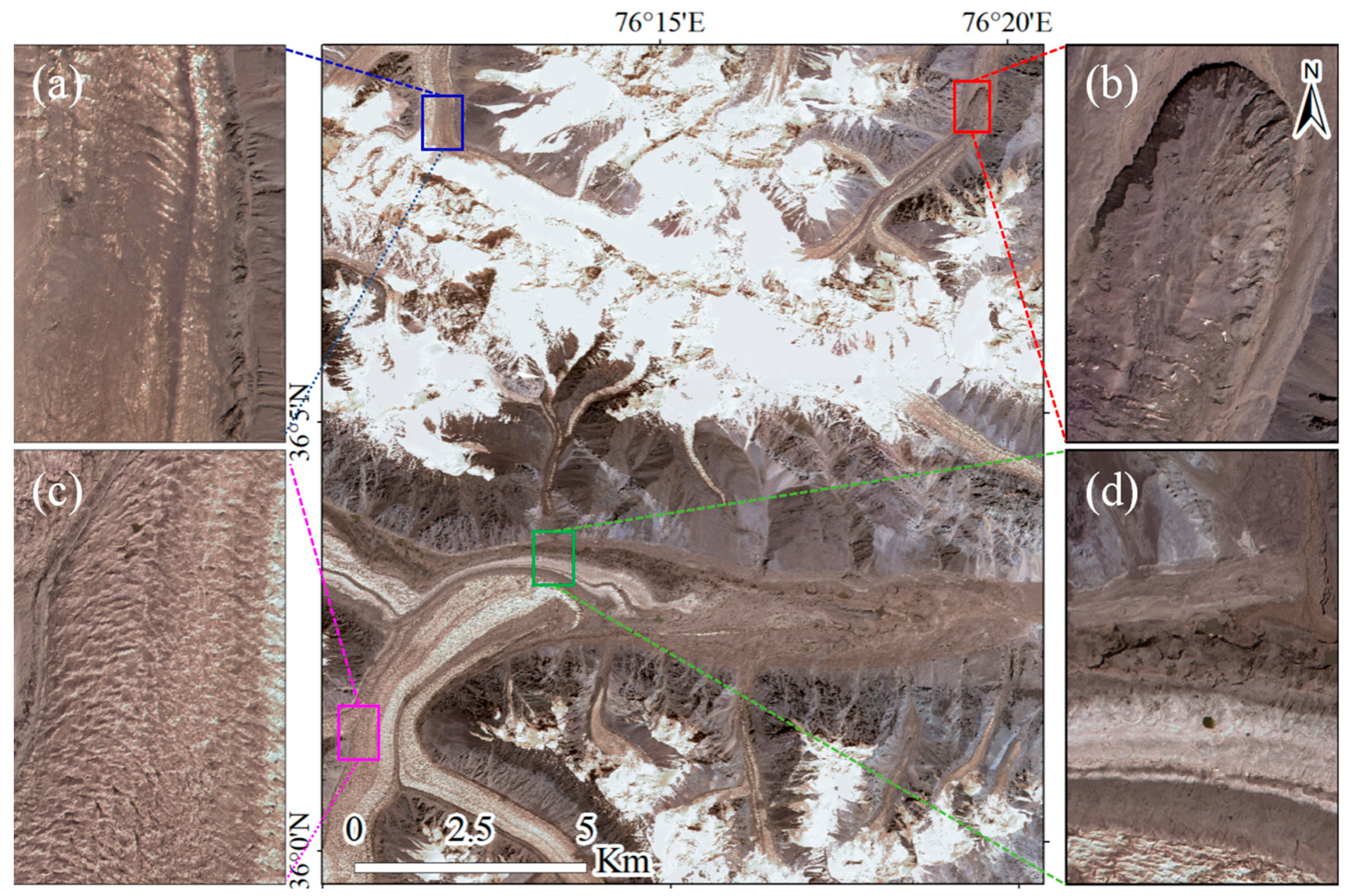
The experimental area selected for this study is the central Karakoram (Figure 1). It has abundant supraglacial debris-covered glaciers, with approximately 14.3% of the total glacier area in this region being covered by supraglacial debris [50,51]. Superglacial debris is expanding and slowing the rate of glacial melt [51].
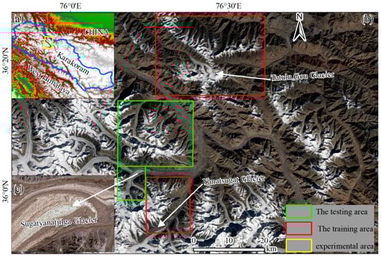
Figure 1.
The central Karakoram study area. The training dataset was obtained from the area in the red boxes; the green boxes mark the test data region. (a) The study area of the High Mountain Asia DEM. (b) The Landsat 8 RGB image. (c) The GF-2 RGB image.
2.2. Datasets
In this study, various remote sensing images were employed to extract glaciers and supraglacial debris in the central Karakoram. The utilized datasets included GF-2, Digital Elevation Models (DEMs), Landsat 8 OLI_TIRS maps, and debris-covered glacier extents from the Karakoram glacier inventories (KGIs) [17]. Table 1 presents detailed information on the datasets, presenting their spectral band, spatial resolution, products, date, and access link.

Table 1.
Datasets used in this study.
2.2.1. GF-2 Images
The high-resolution imagery from the GF-2 satellite serves as crucial data for the extraction of debris-covered glaciers. Launched by China in March 2015, this satellite is equipped with two sensors: a 1 m resolution panchromatic sensor and a 4 m multispectral sensor. To enhance the quality of the GF-2 image data, several preprocessing techniques were applied, including ortho-correction [52], radiometric calibration, atmospheric correction [53], and image fusion. The image fusion technique employed was nearest-neighbor diffusion-based pan-sharpening (NNDiffuse Pan-Sharpening), yielding a synthesized image with a spatial resolution of 1 m [54]. The processed images were then used to extract spectral features for delineating supraglacial debris and glacier outlines.
2.2.2. Landsat OLI_TIR Images
LST plays a crucial role in distinguishing between glacier and off-glacier regions. In this study, we used the radiative transfer equation for the LST inversion of Landsat8 OLI_TIR images to obtain LST. The Landsat8 thermal infrared imaging possessing a spatial resolution of 100 m was resampled to 30 m using a cubic convolution interpolation algorithm [55,56,57]. The Landsat8 OLI_TIR images we used were taken in September 2020; to align the resolution of the images spatially with the GF-2 images, we employed the nearest-neighbor interpolation method for resampling [29,58,59].
The inversion of LST involves the application of the radiative transfer equation [56,60,61]. This process includes multiple sequential steps, such as calculating the NDVI and vegetation cover [58,62,63], determining surface-specific radiance, acquisition of thermal infrared band brightness images, calculation of blackbody radiance brightness at equivalent temperatures, and eventually calculating the LST.
2.2.3. ASTER GDEM
To obtain the topographic characteristics of both the glacier and supraglacial debris, we utilized the ASTER GDEM V3 dataset to compute slopes. The DEM was resampled to 1 m resolution using the method described above in the same way as for LST [59,64,65], and slope was obtained by calculating the ratio of the height difference to the horizontal distance. The distribution of the glacial and debris-covered portions shows significant elevational differences. Glaciers are mostly concentrated at an altitude of 5300–5700 m, while supraglacial debris is mainly distributed at an altitude of 4000–5000 m. The slope of glaciers is mainly concentrated between 0 and 50° [17].
2.3. Algorithm for Mapping Supraglacial Debris
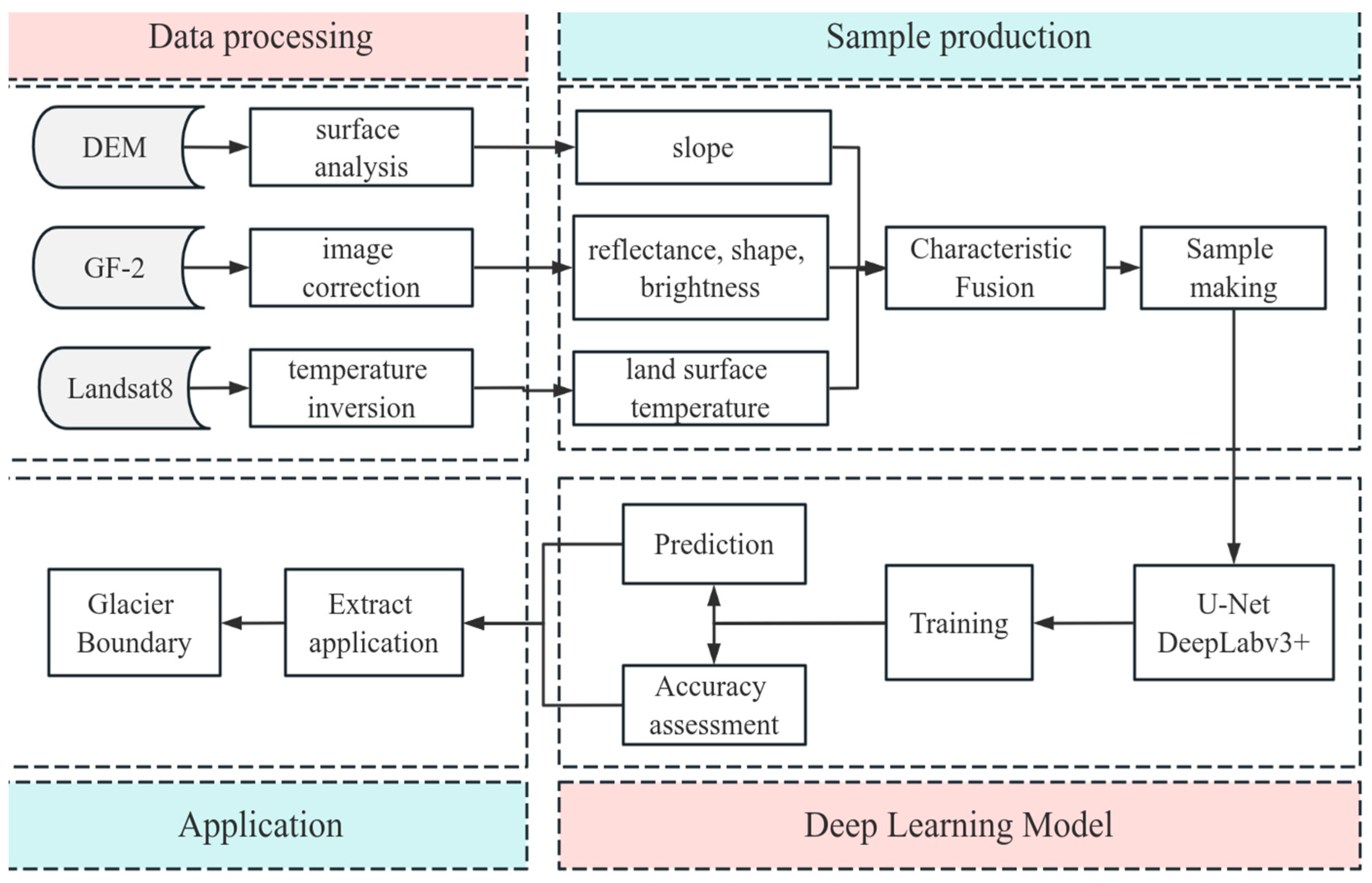
Glaciers can be accurately identified through the analysis of spectral variations, encompassing characteristics such as reflectance, shape, and brightness, among others [66], while the combination of slope and LST facilitates the delineation of supraglacial debris in non-glacial areas [41,47]. The utilization of deep learning models facilitates the identification of disparities at the deep feature level, allowing for the delineation between glaciers, supraglacial debris, and non-glacier regions [67]. The extraction process for glaciers and supraglacial debris from high-resolution images utilizing deep learning is summarized in Figure 2. It includes four main steps: (1) data processing and sample production, (2) model construction, (3) application of glacier and supraglacial debris boundary extraction, and (4) evaluation of accuracy.
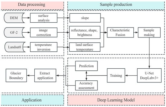
Figure 2.
Framework of debris-covered glacier mapping in this study.
2.3.1. Training Samples
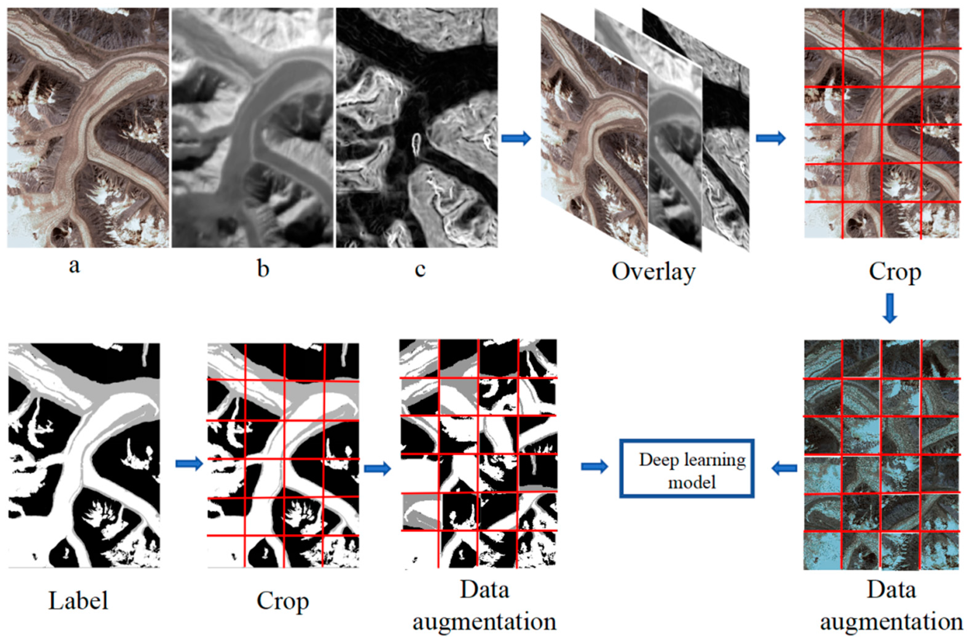
Deep learning heavily relies on the size and quality of training samples. The morphological characteristics of glaciers and the supraglacial debris can be observed in greater detail through high-resolution imagery. Additionally, it is essential for the training samples to encompass a variety of features (glacial and non-glacial). To facilitate the integration of different datasets for deep learning purposes, we uniformly cropped slope, LST, and GF-2 images by sliding window cropping with a zero repetition rate, resulting in a consistent size of 512 × 512 pixels. These images were subsequently fused together. Figure 3 outlines the process of generating the samples. We applied horizontal flipping, vertical flipping, and diagonal mirroring to expand the sample dataset, thereby improving model accuracy and generalization abilities. The dataset consists of 3800 annotated images sized 512 × 512, including the RGB band, slope, and LST across five bands. The dataset was divided into subsets at an 8:1:1 ratio, with 80% (3000 images) allocated for the training set, 10% (400 images) for the validation set, and another 10% (400 images) for the test set. Figure 4 shows sample examples.
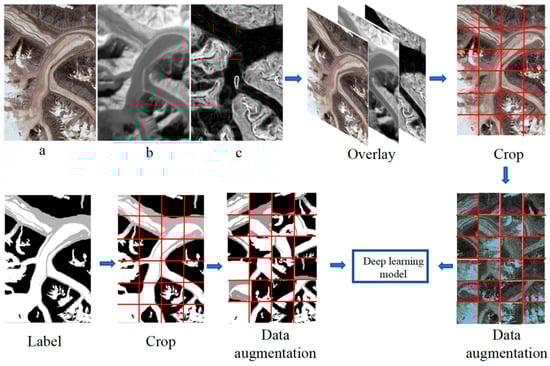
Figure 3.
The procession of Sample production. Sample subset data on the composite image of GF-2 (a), LST (b) from Landsat 8, and the slope (c) from ASTER GDEM. The procedure for preprocessing is visually displayed for cropping, labeling, and augmentation based on a sample chip size of 512 × 512.
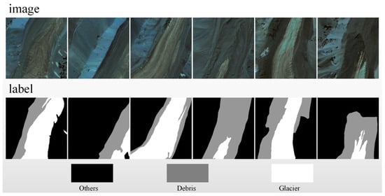
Figure 4.
Partial training samples. The RGB image is in the top half and manually labeled true values are in the bottom half. In the labeled sections, gray sections represent supraglacial debris, white sections represent glaciers, and black sections represent non-glacial areas.
2.3.2. Deep Convolutional Networks
Three convolutional neural networks (FCNN, DeepLabV3+, U-Net) were used in this study to map debris-covered glaciers. FCNN, which was first introduced in 2015 [68], operates at a pixel level for semantic segmentation. We implemented the FCNN architecture based on the Visual Geometry Group (VGG16) Network [69] in this study. The FCNN exhibits a more streamlined model architecture and requires less time for training. DeepLabV3+ [34] is an evolution of the DeepLabv3 model [70]. The DeepLabv3+ model exhibits a higher level of complexity in its structure and requires more training time and training samples. The Atrous Spatial Pyramid Pooling (ASPP) module enhances the receptive field of the model, thereby enabling it to capture a broader spectrum of image features during the feature extraction process. We used Xception and ResNet-34 [71] as the backbone of the DeepLabv3+ model and integrated a CBAM [72] to enhance the weighting of delineation for debris-covered glaciers (Figure S1a). U-Net utilizes skip connections and a decoder with multi-upsampling layers to capture both low- and high-level information [33]. For further feature extraction, we incorporated four additional convolutional layers into the effective feature layer of U-Net networks. CBAM was also integrated to increase the recognition weight of the target pixels (Figure S1b).
CBAM represents a fundamental yet potent addition to feed-forward convolutional neural networks. Through the integration of the Spatial Attention Module (SAM) and the Channel Attention Module (CAM), CBAM significantly augments object recognition capabilities and has demonstrated cutting-edge performance across a spectrum of computer vision tasks [72]. CBAM processes attention maps through the CAM and SAM (Figure S2). These resultant attention maps are then efficiently combined with input feature maps, enabling the ability to perform adaptive tuning for optimization.
Cross-entropy loss function: This particular function serves to gauge the disparity between predicted outcomes and the actual labels. By minimizing the value of this loss function, the predictions of the model are expected to align more closely with the real labels, thereby greatly improving the classification capabilities of the model [73]. The calculation of the cross-entropy loss function is represented in Equation (1), where the actual sample distribution is denoted as yc, and the predicted distribution is represented as Pc.
Optimization function: The process of fine-tuning model parameters through an optimization algorithm, known as updating model weights, is crucial for minimizing the loss value. In our study, we employed the Adam optimization function [74]. Adam is an algorithm specifically designed to efficiently handle first-order gradient optimization for stochastic objective functions. This method has been particularly effective in addressing challenges encountered in local deep learning problems, especially when dealing with large datasets and complex models.
Activation function: Since our research involves a complex task of multi-classification, specifically the distinction between supraglacial debris and glaciers, we adopted the softmax activation function to establish probability distributions across different categories. The softmax function non-linearly maps the characteristics of individual pixels to their respective categories, assigning weightings to each category. This transformation converts the output value of each pixel into a probability distribution, ensuring positive values that together sum up to 1; the category with the highest probability is selected as the classification outcome for that pixel [75]. The confidence level assigned to each class is determined by the probability distribution of the pixel, which reflects the number of classes associated with the respective label, as shown in Equation (2).
2.3.3. Network Optimization Using CBAM
We incorporated CBAM into U-Net and DeepLabV3+, emphasizing the importance of the features for debris-covered glaciers [72,76,77]. While the spatial pyramid pooling module of DeepLabV3+, which utilizes dilated convolutions, excels at capturing contextual information at different scales, it may introduce spatial discontinuities [34]. This challenge is effectively addressed by integrating CBAM into the feature extraction process. Moreover, the integration of CBAM enables the extraction of more contextual information by capturing low-level features from the backbone network. To overcome the information loss caused by the pooling layer in the U-Net network, CBAM is incorporated after the initial feature extraction phase. This incorporation enables the extraction of important low-level features, thereby ensuring that the feature fusion process encompasses more crucial information.
2.3.4. Model Evaluation Indices
In order to evaluate the results of the deep learning model in identifying debris-covered glaciers in high-resolution images, we performed quantitative analyses on the test set. These analyses utilized accuracy evaluation metrics based on a confusion matrix (Table S1) [78], specifically including accuracy, F1 score [79], mean intersection over union (MIoU) [80], and kappa statistics [81].
Accuracy refers to the proportion of the model’s mapped number of samples compared to the total number of samples. A higher accuracy indicates a better model. The formula for accuracy is as follows:
where TP indicates a true positive, FP indicates a false positive, FN indicates a false negative, and TN indicates a true negative.
The F1 score takes into account both checking accuracy and checking completeness, enabling the two seemingly contradictory metrics of precision (P) and recall (R) to be maximized and balanced simultaneously [79,82].
Kappa is a metric for assessing the degree of agreement between predictions and actual observed values [81,83]. The formula is given as follows:
where represents the proportion of accurately classified samples in each category, while the overall classification accuracy is determined by the ratio of correctly classified samples to the total number of samples. is calculated as the sum of the products of the actual and predicted numbers assigned to all categories, divided by the square of the total sample size (see Equation (6)), where n denotes the overall sample size.
The MIoU is computed as the sum and average of the intersection and merger ratios for every category, as shown in Equation (7), where n refers to the total number of samples.
3. Results
3.1. Experimental Setup
The experiments were conducted on a Windows 11 64-bit operating system and the Python programming implementation, which was equipped with an experimental device comprising a 13th generation Intel® Core™ i5-13490F (2.50 GHz) central processing unit (CPU) and 64 GB of random-access memory (RAM). For the purpose of graphical computations, an Nvidia GeForce RTX 4070 graphics card with 12 GB of memory was employed. TensorFlow became the preferred deep learning framework with version 2.6.0, while CUDA version 11.2 became the foundation of GPU computation. cuDNN8.1 facilitates the acceleration of the deep learning GPUs, improving the computational efficiency and performance.
3.2. Accuracy Comparison between Different Models
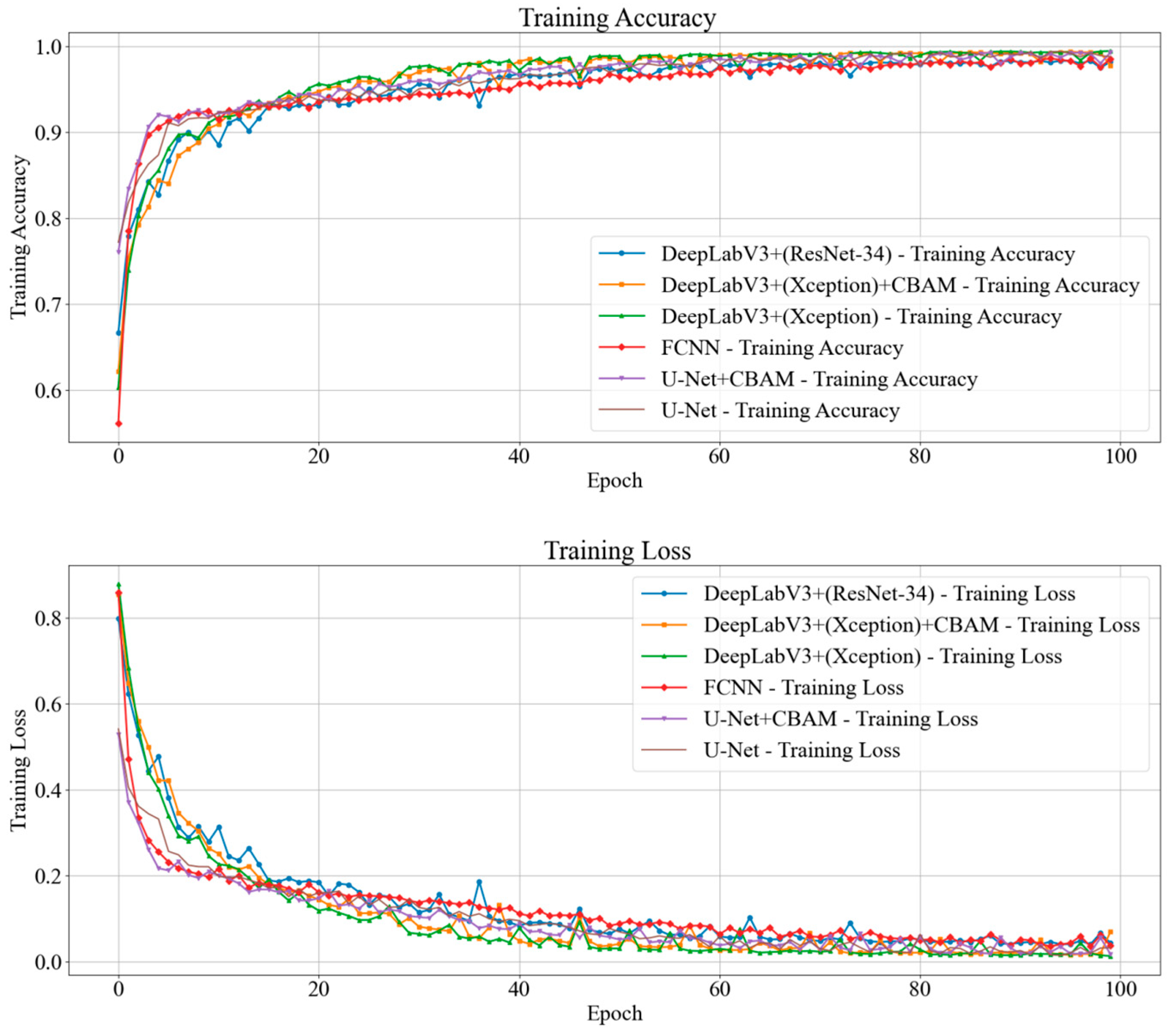
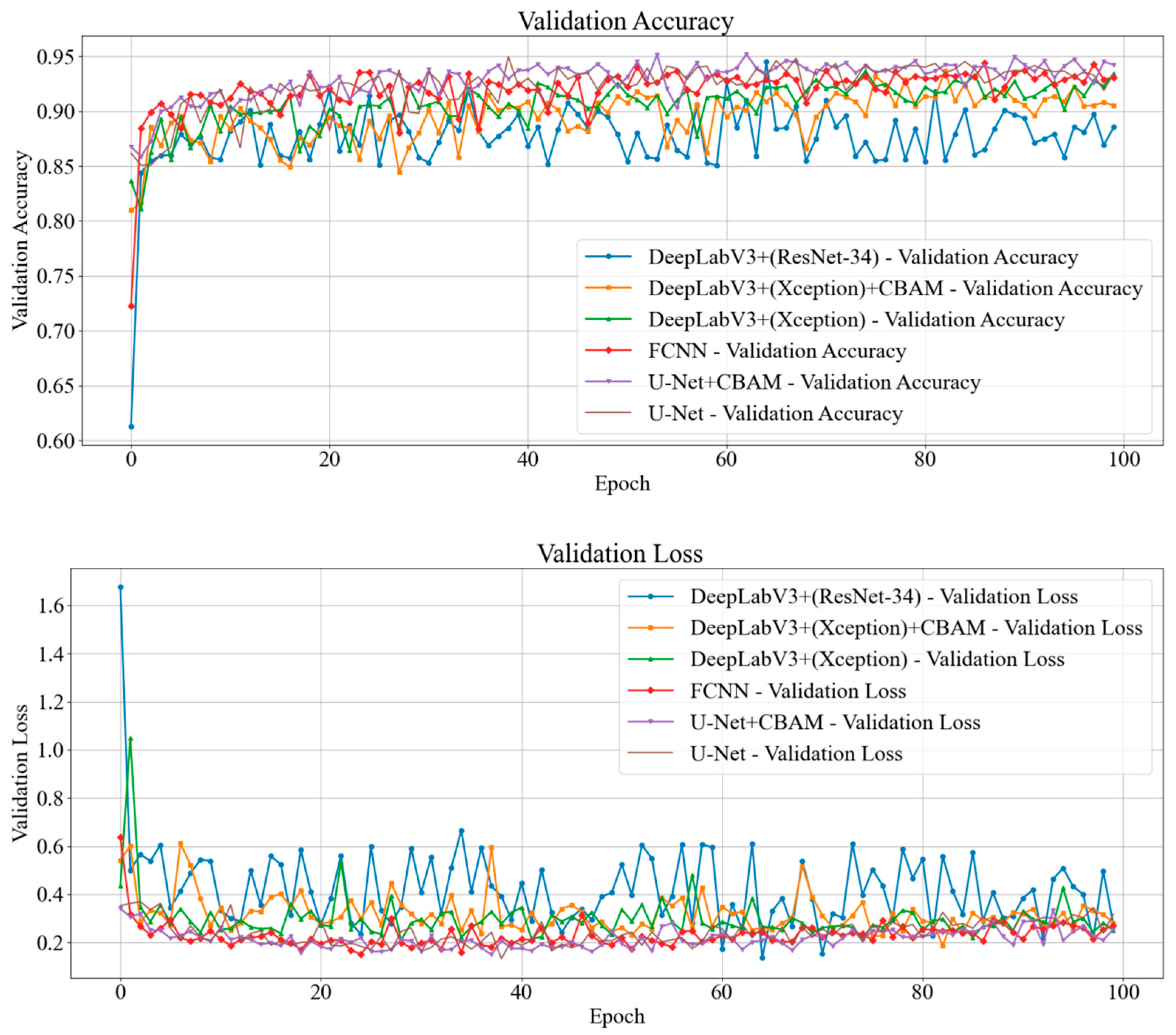
The dynamics of loss and accuracy variations depict the iterative process of adaptive model refinement [31]; higher accuracy implies lower loss. Monitoring the fluctuations in loss and accuracy of the validation set offers insights into the ability to fit the data of the model and the effectiveness of its feature extraction. The achievement of a stable trend in accuracy and loss indicates the completion of model training. In this study, six deep convolutional neural network models, including FCNN, U-Net, and DeepLabV3+, underwent training for 100 epochs. Figure 5 and Figure 6 visually depict the progression of accuracy and loss across training epochs for each model. The FCNN and both U-Net and U-Net with CBAM showed high fitting accuracy, with U-Net utilizing CBAM showcasing the most precise fitting (99.3% and 95.2% for training and validation sets, respectively). However, for DeepLabV3+ and its associated models, relatively suboptimal fitting performance was observed, presenting relatively lower accuracy, with validation accuracies around 92%. In addition, DeepLabV3+ utilizing the ResNet-34 backbone showed large fluctuations in accuracy on the test set, and the fit was the worst of all the models (Figure 6).
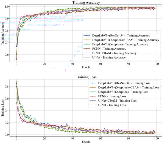
Figure 5.
Different model training accuracy and loss changes. The upper half is the training accuracy and the lower half is the training loss. The horizontal coordinate represents the epoch, with a total of 100 epochs. The extent of convergence of the model can be deduced by observing the fluctuation in accuracy.
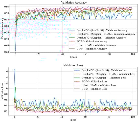
Figure 6.
Different model validation accuracy and loss changes. The upper half is the validation accuracy and the lower half is the validation loss. The horizontal axis represents the number of training iterations.
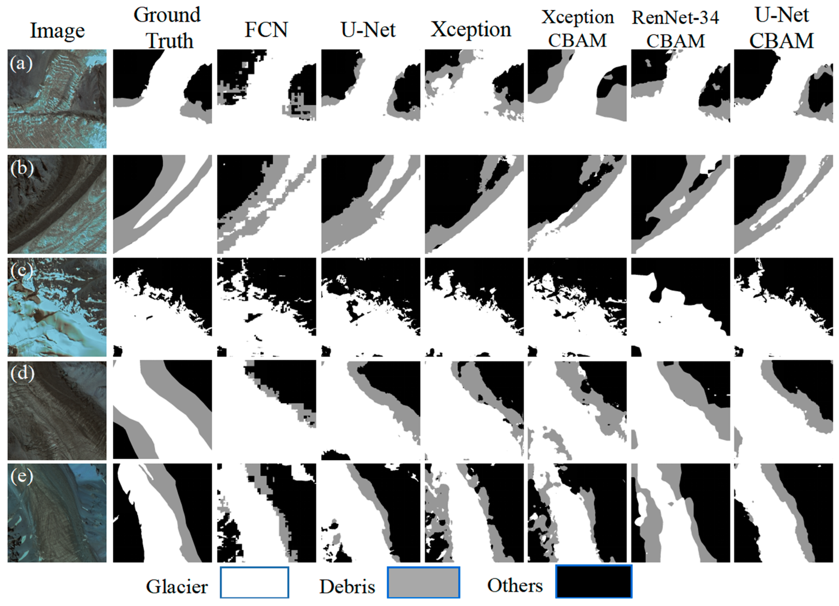
The visualization results for the predictions are shown in Figure 7. It is worth noting that DeepLabv3+ using Xception and ResNet-34 as backbone networks displays suboptimal performance on the test set (Figure 7, columns 5 to 7), likely due to the limited feature extraction capabilities inherent in these selected backbone networks. FCNN produces commendable results in extraction of bare ice; however, the delineation of supraglacial debris exhibits fragmentation (Figure 7, column 3). Conversely, U-Net demonstrates proficient extraction capabilities for supraglacial debris (Figure 7a,e); nevertheless, it occasionally misidentifies other features as glaciers. After the integration of CBAM, a noticeable reduction in the effects of seasonal snow cover is observed (Figure 7c), resulting in smoother and fewer identified supraglacial debris patches (Figure 7b,d,e). This enhancement illustrates that U-Net incorporating CBAM exhibits superior proficiency in extracting supraglacial debris-covered glaciers, displaying reduced susceptibility to other features while extracting glacier boundaries characterized by greater continuity and fewer intricate patches.
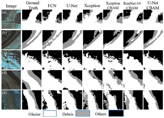
Figure 7.
Visualization of the prediction results of the different models on the test set. (a,b) Bare ice boundaries are clearly visible. (c) Covering seasonal snow. (d,e) The sample contains cryoconite with an unclear boundary with the supraglacial debris; Xception and ResNet-34 are representative of DeepLabV3+ for different feature extraction networks, respectively. CBAM denotes the introduction of the Convolutional Block Attention Module.
Table 2 presents a comprehensive overview of metrics, such as accuracy, F1 score, kappa, and MioU, computed for different models on the test set, with values ranging from 0 to 1. The evaluation of six models demonstrated that U-Net achieved the highest accuracy in recognition, particularly when integrated with CBAM. It achieved accuracy, F1 score, MIoU, and kappa values of 0.931, 0.742, 0.794, and 0.877, respectively. Following closely, FCNN (0.899, 0.630, 0.717, 0.818) and DeepLabv3+ with Xception as the backbone and CBAM (0.903, 0.593, 0.714, 0.826) emerged as the second-ranked models. These models exhibited similar accuracy, MIoU, and kappa values, with marginal differences of approximately 0.4%, 0.3%, and 0.8%, respectively. Notably, while DeepLabv3+ displayed comparable accuracy, MIoU, and kappa values, it slightly lagged behind FCNN in supraglacial debris recognition (F1 score of 0.593, 3.7% lower than FCNN). Conversely, DeepLabv3+ with Xception and ResNet-34 backbones exhibited lower accuracy in supraglacial debris identification (Table 2) with F1 scores of 0.41 and 0.551, and struggled to accurately capture supraglacial debris boundaries. In summary, U-Net integrated with CBAM demonstrated the highest extraction capability. While the models associated with DeepLabv3+ showed relatively weaker performance in the extraction of supraglacial debris, they exhibited stronger extraction abilities for bare ice. This discrepancy arises from their overall accuracy, MIoU, and kappa values being comparable to those of other models but their F1 scores being revealed as lower, specifically for supraglacial debris.
Table 2.
The test set accuracy of various models for recognizing supraglacial debris.
3.3. Mapping of Debris-Covered Glaciers at the Regional Scale
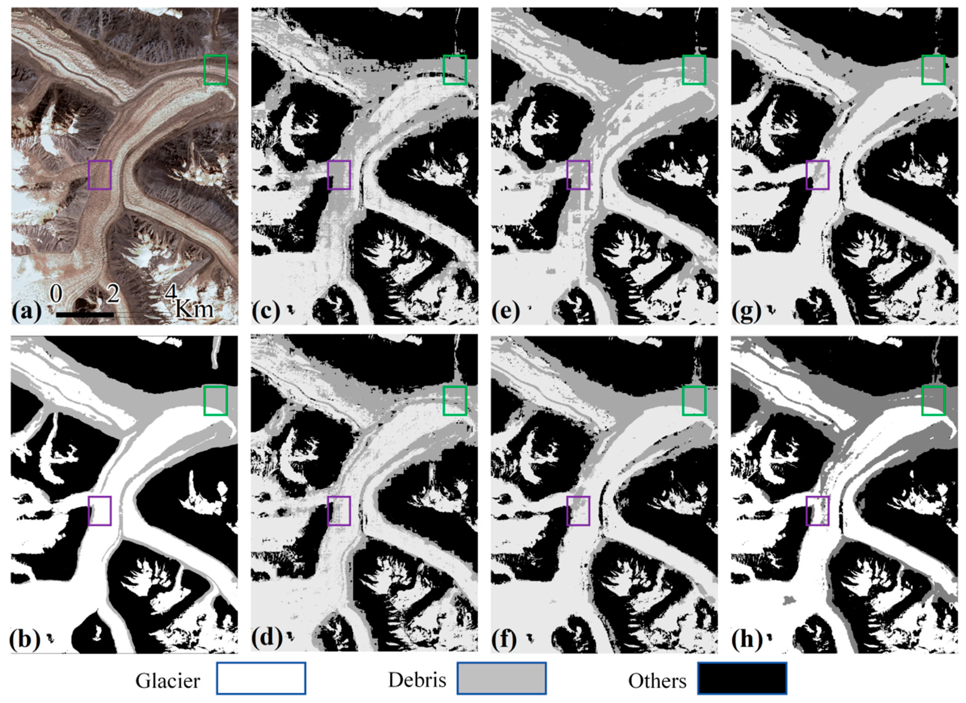
In this section, the models were tested based on two scenes of GF-2 images, in order to assess the effectiveness of various techniques, including DeepLabv3+, U-Net, U-Net with CBAM, and others, in the extraction of debris-covered glaciers with different properties at a regional level. The results for each approach are visually presented in Figure 8 and Figure 9, with manually revised ground truth values serving as benchmarks.

Figure 8.
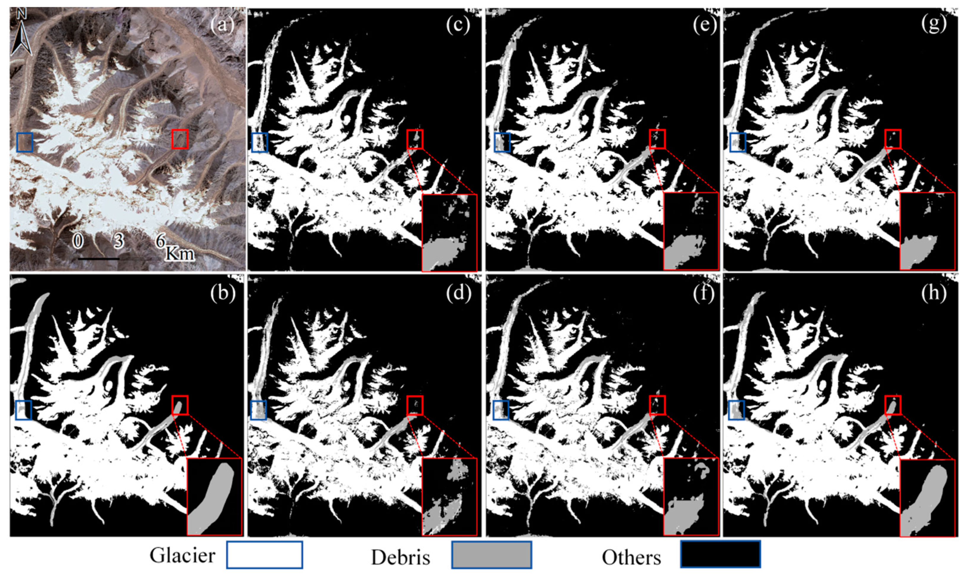
Visualization of debris-covered glacier extractions at glacier terminus. (a) The GF-2 image, (b) the ground truth, (c) DeepLabV3+(Xception), (d) DeepLabV3+(Xception)+ CBAM, (e) DeepLabV3+(ResNet-34)+ CBAM, (f) FCNN, (g) U-Net, (h) U-Net with CBAM. The green and purple boxes represent high-reflectivity debris and glaciers with cryoconite or weak fouling, respectively.
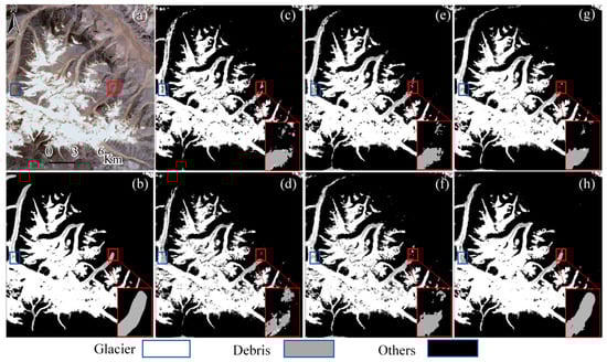
Figure 9.
Visualization results of debris-covered glacier extraction in the predicted region. (a) The RGB image, (b) the ground truth, (c) DeepLabV3+(Xception), (d) DeepLabV3+(Xception)+ CBAM, (e) DeepLabV3+(ResNet-34)+ CBAM, (f) FCNN, (g) U-Net, (h) U-Net with CBAM. The red and blue boxes represent low-reflectivity debris and mixed-type supraglacial debris, respectively.
The supraglacial debris can be classified based on its reflectivity; we distinguish between low-reflectivity debris composed predominantly of mineral or clay particles (Figure 10b) and high-reflectivity debris with a significant presence of ice crystals or flakes (Figure 10d), as well as their mixes (Figure 10a). The extraction performance of different deep learning models varies with regard to the supraglacial debris in question. DeepLabV3+ with Xception as the backbone in our model occasionally misclassified glaciers with cryoconite or weak fouling (Figure 10c) as supraglacial debris (purple box in Figure 8c), resulting in fragmented shapes in the identification of supraglacial debris. The integration of CBAM improved the overall recognition, yielding smoother results, particularly enhancing the accuracy in identifying slightly polluted ice surfaces (Figure 8f), but the identification of the supraglacial debris boundary remained uncertain, often presenting fine patchy debris. Employment of ResNet-34 as the backbone network along with CBAM resulted in increased smoothness in the identification of DeepLabV3+, yet misclassification of certain debris-covered bare ice areas as supraglacial debris and a higher occurrence of fine, patchy segments of supraglacial debris were observed (Figure 8e). Compared to DeepLabV3+, the other models such as FCNN, U-Net, and U-Net with CBAM demonstrate superior recognition capabilities for glaciers with cryoconite or weak fouling, yielding distinct boundary delineations of the supraglacial debris (Figure 8f–h). In addition, highly reflective supraglacial debris (Figure 10d) is well represented in all of our models (see green box in Figure 8). However, for the extraction of low-albedo supraglacial debris (Figure 10b) and mixed-type supraglacial debris (Figure 10a), all models, except for U-Net with CBAM, produced incorrect results (see red and blue boxes in Figure 9). These results can be attributed to the different levels of model attention to specific features. The U-Net and FCNN models are more sensitive to temperature features, which allows them to effectively distinguish between supraglacial debris in glacial regions. In contrast, the DeeplabV3+ model falls short in recognizing supraglacial debris with similar slopes and spectra. Furthermore, the model is unable to distinguish between bare ice and glacial debris with high reflectivity. This may be attributed to the model’s lack of attention to temperature, with a greater focus on spectra and slope.

Figure 10.
Identification of supraglacial debris with different reflectance characteristics. (a) Mixed types of supraglacial debris, (b) low-reflectivity debris composed predominantly of mineral or clay particles, (c) glaciers with cryoconite or weak fouling, (d) high-reflectivity debris with a significant presence of ice crystals or flakes.
It is worth noting that, compared to the extraction performance of the test set, all models demonstrated improvements in extraction accuracy at the regional scale. Specifically, U-Net with CBAM exhibited notable enhancements in accuracy, F1 score, MIoU, and kappa by 1%, 12.2%, 7%, and 2.8%, respectively (reaching 0.941, 0.864, 0.864, and 0.905). These metrics surpassed those of U-Net (0.908, 0.773, 0.791, 0.851) and FCNN (0.907, 0.781, 0.793, 0.849). However, DeepLabv3+ and its related models continued to achieve comparatively lower accuracy in this regional-scale evaluation.
The glacier segmentation involves the intricate task of delineating complex glaciers into individual units. Our segmentation process involves the utilization of ridge line data generated and manually refined based on the ASTER GDEM v3 dataset [17,47,84]. We conducted a comparative analysis of area statistics post-segmentation for three glaciers using various models (Figure 11). The discrepancies in area measurements between the extraction outcomes for bare ice obtained through U-Net with CBAM and the artificially revised true values were minimal. They ranged between 0.01 and 0.03 km2. On the other hand, the variation in the extracted surface size of supraglacial debris showcased a slightly wider range, varying between 0.03 and 0.13 km2; this model demonstrated the least area variation (Figure 11). It is important to note that the correlation models associated with DeepLabv3+ exhibited considerable variability in the extent of extracted supraglacial debris. However, in contrast, the differences between the models in the area of bare ice extracted were relatively smaller and more consistent (Figure 11).
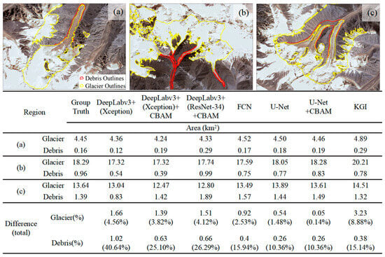
Figure 11.
Comparison of area statistics extracted by various models on typical glaciers. It includes areas of individual and summed bare ice and supraglacial debris, differences in total area extracted by distinct models, and corresponding percentages. (a–c) Glacier units segmented by ridge lines.
4. Discussion
4.1. Comparison with Previous Glacier Outlines
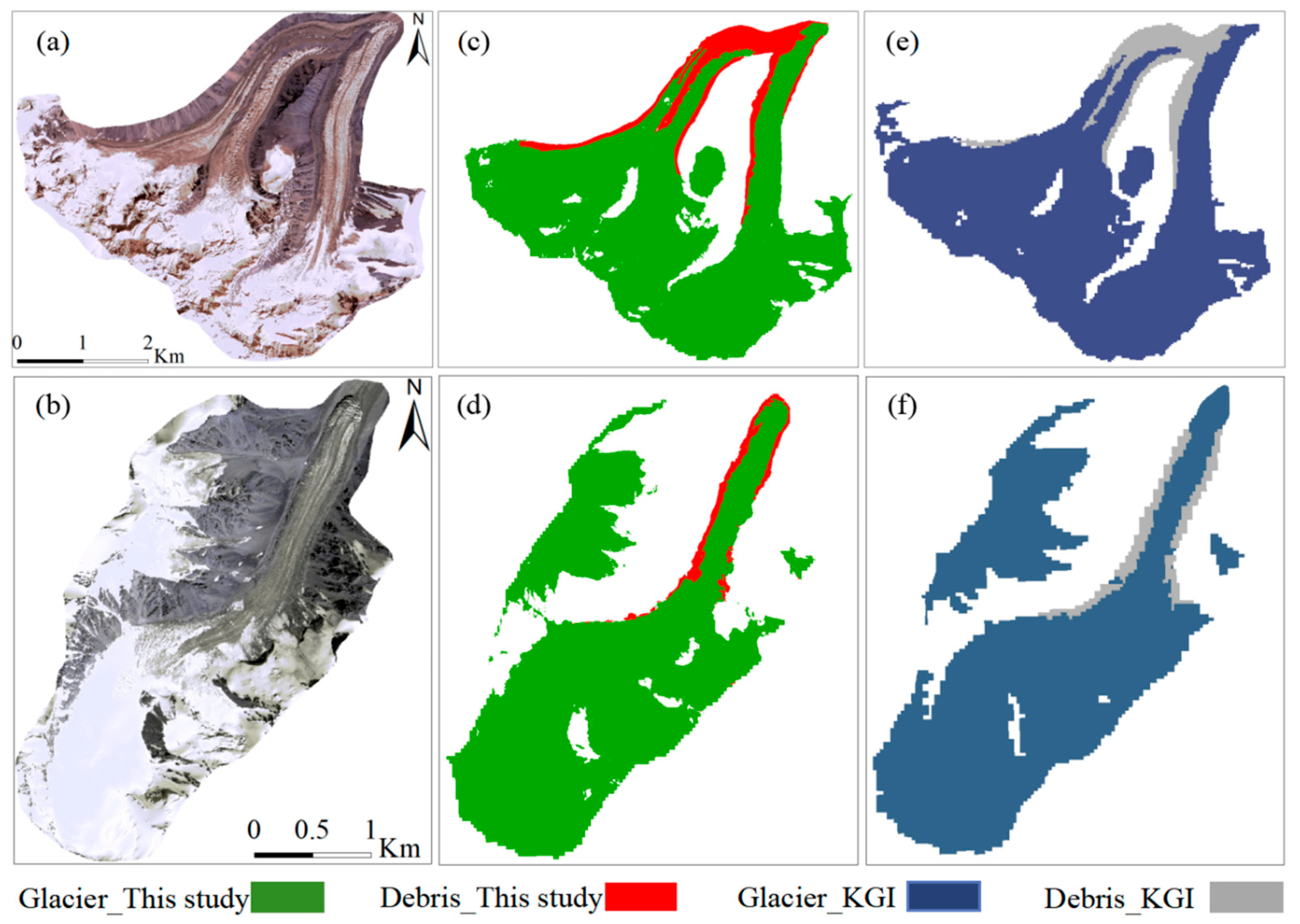
Accurate glacier inventories play a crucial role in accurately assessing the volume, mass balance, and length measurements of glaciers [85]. The utilization of high-resolution imagery for the generation of glacier inventories will reduce the uncertainty of the glacier inventories, thereby providing greater assurance of the accuracy of related studies. In contrast to the multi-temporal Karakoram glacier inventories (KGIs, 2018–2020) compiled by Xie, which based on Landsat TM/ETMC/OLI imagery [17], our results exhibit a high level of similarity to the KGIs in terms of shape (Figure 12 and Figure 13), while also providing more detailed boundaries (Figure 13). It is worth noting that our extraction in typical glacier areas differed from the KGIs by 1.38 km2 (7.78% of the extraction area) and in supraglacial debris by 0.07 km2 (4.19% of the extraction area). This discrepancy can be attributed to the inadequate differentiation of the KGIs between exposed rock areas on the glacier (see Table 3). From the perspective of data sources, our data were obtained from 1 m resolution GF-2 panchromatic and multispectral images, supplemented with terrain and temperature features. The KGIs were produced by imagery at a 30 m spatial resolution. The use of higher-resolution imagery results in fewer mixed pixels, allowing for a clearer differentiation between features and enabling a more detailed classification of glaciers, supraglacial debris, and other types of terrain. This finer resolution significantly enhances the precision of boundary extraction.

Figure 12.
The results of our extraction on typical glaciers are compared with the KGIs. (a,b) An RGB image of a typical glacier, (c,d) our extraction results, (e,f) the KGI glacier range.
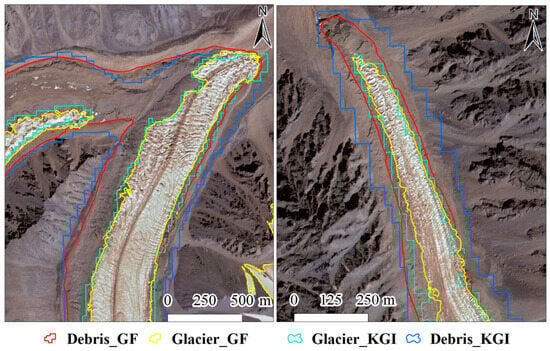
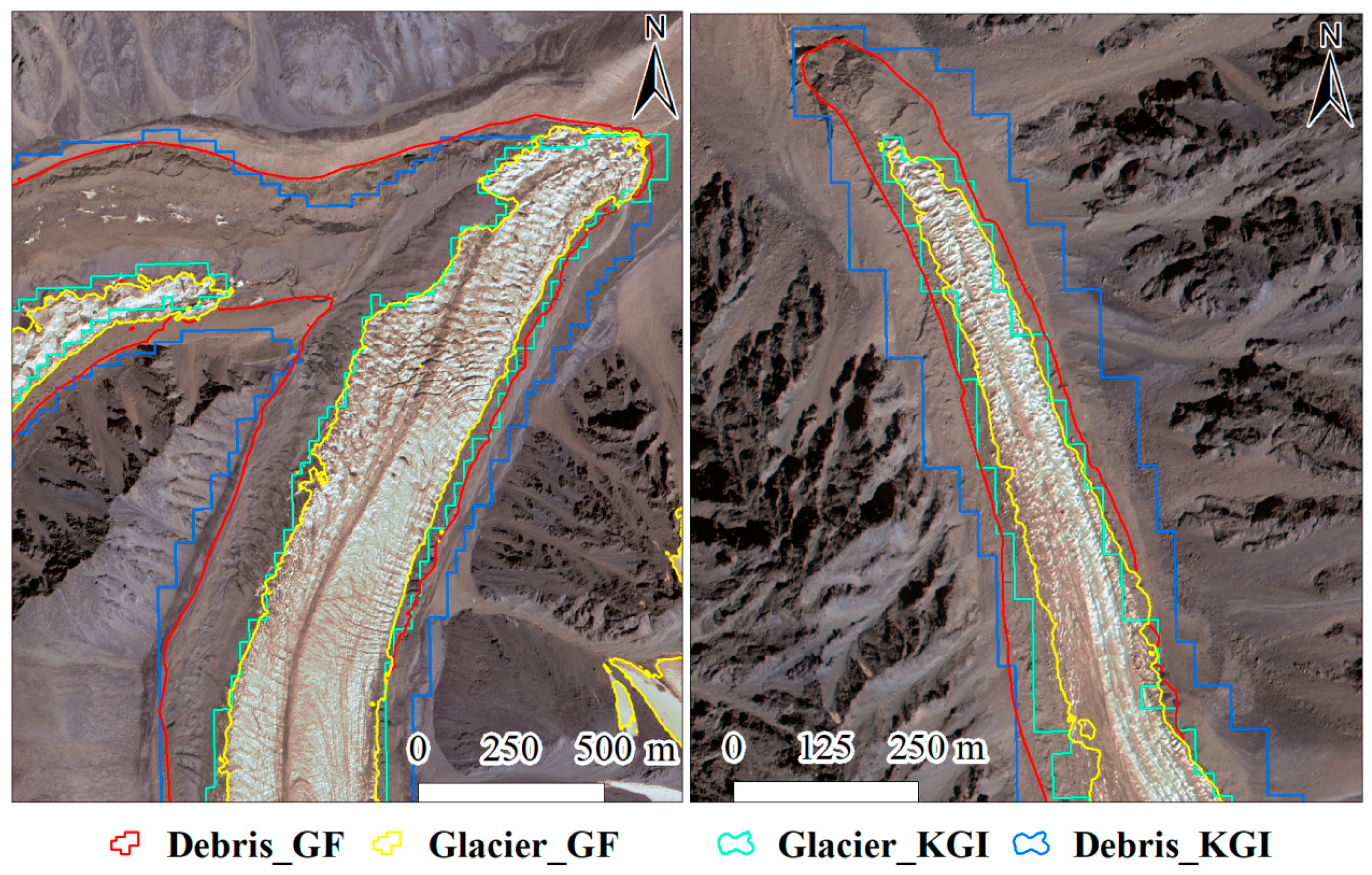
Figure 13.
Comparison of our results with the KGI at the end of the glacier. KGI refers to the Karakoram glacier inventories produced in 2023.
Table 3.
Comparison of the extraction results for typical glaciers with the area of the KGIs.
4.2. Effects of Different Feature Combinations on Supraglacial Debris Identification
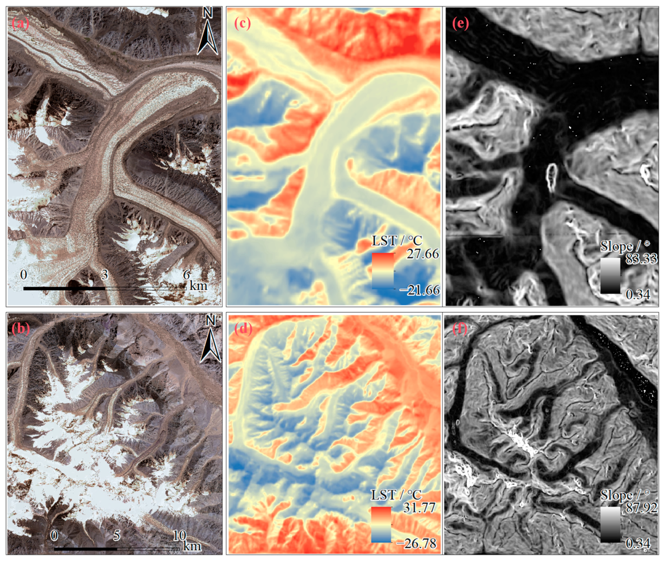
In glacial regions, the delineation of boundaries between debris-covered glaciers and bare ice zones poses a challenge due to the difficulty in differentiating glacial dust and debris-covered areas [37]. This task is further complicated by the presence of non-glacial areas like frozen lakes and rivers, which also hinder this boundary extraction [37,86,87]. To address this issue, our study employs slope and LST as indicators to differentiate between debris-covered glaciers and various features like debris, valleys, rocks, and rivers. By analyzing the spatial distribution characteristics (Figure 14), we find that the LST of glacial regions is primarily below 13 °C, with most bare ice areas having an LST below 0 °C, while the supraglacial debris is concentrated in the range of 0–13 °C. The LST of non-glacial areas is predominantly above 13 °C, and some non-glacial features that are closer to the glacier or contain non-glacial snow have LSTs of 4–13 °C. In terms of slope, the glacial area has a predominant concentration of slopes between 0 and 50°, whereas supraglacial debris are predominantly found in areas below 20°. The differences in LST and slope between glaciated and non-glaciated areas are crucial for the extraction of supraglacial debris-covered glaciers. To explore the role of each feature in glacier extraction, we trained our deep learning model with different combinations of features to evaluate their effectiveness in accurately identifying debris-covered glaciers (see Figure 15).
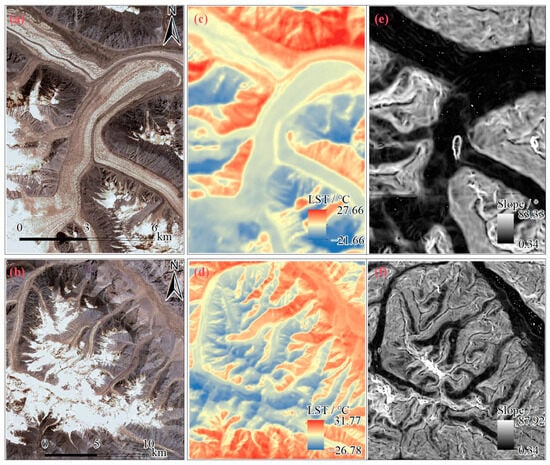
Figure 14.
Spatial distribution characteristics of LST and slope in glaciated and non-glaciated areas. (a,b) The GF-2 images of the test area. (c,d) LST: the LST of glacial regions is primarily below 13 °C, with most bare ice areas having an LST below 0 °C. (e,f) Slope: the glacial area has a predominant concentration of slopes between 0 and 50°.
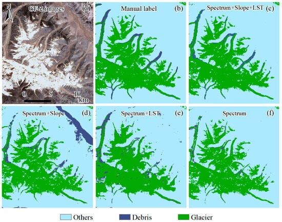
Figure 15.
Extraction results of different metrics based on U-Net with CBAM. (a) GF-2 images of the test area. (b) Manually revised true values. (c) Results of metric extraction, combining spectrum with slope and LST. (d) The results of the extraction are derived from a combination of spectral and slope features. (e) The results of the extraction are derived from a combination of spectral and LST features. (f) Extraction results from the combination of spectral features.
While slope plays a crucial role in distinguishing supraglacial debris from bare rock areas, the interference from rivers leads to misidentification, resulting in a visible discrepancy compared to the actual values (Figure 15d). This discrepancy may arise from spectral and slope similarities between rivers and supraglacial debris regions. LST proves to be effective in distinguishing between bare ice and supraglacial debris; however, it tends to misclassify bare rock areas within glacial regions as supraglacial debris, thereby overestimating the extent of the debris-covered area compared to the actual values (Figure 15e). Remarkably, when both slope and LST features are absent, only bare ice can be identified, and the model has the lowest capability of supraglacial debris extraction (Figure 15f). We conducted calculations to determine the recall rate of each index for the purpose of supraglacial debris extraction (Table 4). Our experiments revealed that the recall rate is at its lowest when solely using the spectrum. However, incorporating both slope and LST alongside the spectrum has been shown to enhance the accuracy of moraine extraction. Specifically, when all three indices, namely spectrum, slope, and LST, are combined, the recall rate reaches its peak, resulting in the highest level of accuracy for supraglacial debris recognition. The presence of seasonal snow presents challenges in accurate glacier boundary extraction [37,38]. Fortunately, the high-resolution imagery data utilized in our study, obtained from the August 2020 GF-2 satellite imagery, exhibited minimal seasonal snow and cloud cover, and our methodology demonstrates a certain capability to exclude small amounts of non-glacial snow. It is worth noting that the original resolution of the terrain and temperature features used in our study differs from that of the GF-2 satellite imagery. This discrepancy may to some extent increase the complexity of feature extraction for the model, thereby affecting the precision of the extraction.
Table 4.
Comparison of the recall for the various indicators in extracting glacial and supraglacial debris.
4.3. Advantages in Debris-Covered Glacier Mapping
The selection of high-resolution imagery for this study has expanded the available geographic information, offering a wider range of spectral features while simultaneously amplifying the challenge in accurately extracting glaciers and supraglacial debris. Nevertheless, it highlights the robustness of our model. When applied to the typical debris-covered areas in the Karakoram Mountains, our method demonstrated strong capabilities in effectively extracting supraglacial debris and glaciers. Remarkably, the identified boundaries of supraglacial debris exhibited continuity and smoothness, displaying reduced patchiness. The integration of CBAM significantly enhanced feature weighting for glaciers and supraglacial debris, thereby further improving identification accuracy. Unlike previous identification approaches that are based on medium- to low-spatial-resolution data [25,27,42], our methodology emphasizes higher spatial resolution, enabling obtaining more accurate glacier boundaries. In contrast to studies that solely focused on spectral information [38,88,89,90], we integrated crucial terrain and temperature data, which are vital for supraglacial debris identification and, to some extent, the exclusion of non-glacial snow. This method promises the creation of high-precision glacier inventories that include supraglacial debris.
5. Conclusions and Prospects
This study presents a novel approach that combines deep learning semantic segmentation networks with diverse features to accurately identify and extract high-resolution glaciers and supraglacial debris. By addressing the limitations of high-resolution imagery lacking shortwave infrared bands for supraglacial debris identification, this approach enables precise applications in high-resolution settings. The generation of high-quality glacier inventories serves to create a foundational dataset for future refined glacier studies. Six deep learning models were employed to extract debris-covered glaciers. The degree of fit, extraction results, and extraction accuracy of the different models were then discussed and analyzed. Comparative analyses of different model extraction outcomes demonstrate the superior effectiveness of the U-Net model combined with attention mechanisms. This model achieves an accuracy of 94.1%, both an F1 score and an MIoU of 0.864, and a kappa coefficient of 90.5% in typical glacier regions, surpassing the other models employed. Furthermore, comparison with the Karakoram glacier inventory (KGI) and manually annotated label data confirms the proficiency of this method in extracting regional-scale glaciers and supraglacial debris. The eigenvalues of glacial zones were enumerated, and the impact of various features on the extraction of supraglacial debris was validated. It was demonstrated that slope and surface temperature were significant factors in the identification of supraglacial debris. Compared with previous studies, this research makes three primary contributions: (1) the exploration of relevant features suitable for high-spatial-resolution identification of glaciers and supraglacial debris, (2) the integration of attention mechanisms to augment the extraction capabilities of deep learning models like U-Net and DeepLabv3+, and (3) the proposition of a method utilizing multisource, multiband imagery as inputs for deep learning models to extract high-quality glaciers and supraglacial debris.
For future research and improvements, there are three crucial aspects that should be taken into consideration: Firstly, the integration of DEM data obtained from high-resolution imagery could be utilized to calculate terrain factors. This approach has the potential to resolve issues that may arise from using different data sources. Secondly, the diversity within training sample sets could be expanded by incorporating various landforms. This augmentation aims to enhance the capacity of deep learning models by exposing them to a wider range of features, thus increasing the accuracy of the models. Lastly, the model architecture could be refined by optimizing the network structure, selecting more suitable loss functions specifically tailored for the extraction of debris-covered glaciers, and focusing on bolstering the ability of the model to learn features while mitigating the impact of noise elements such as ice lakes, glacier surface rivers, clouds, and mountain shadows on the extraction of debris-covered glaciers.
Supplementary Materials
The following supporting information can be downloaded at: https://www.mdpi.com/article/10.3390/rs16122062/s1.
Author Contributions
Conceptualization, S.L.; Methodology, X.Y., F.X., S.L., Y.Z., Y.D., R.F. and S.G.; Software, X.Y.; Resources, J.F., H.Z. and Y.F.; Data curation, X.Y.; Writing—original draft, X.Y. and F.X.; Project administration, S.L. All authors have read and agreed to the published version of the manuscript.
Funding
This research has been supported by the International Science and Technology Innovation Cooperation Program of the State Key Research and Development Program (grant no. 2021YFE0116800), the Second Tibetan Plateau Scientific Expedition and Research Programme (grant no. 2019QZKK0208), the National Key R&D Program International Science and Technology Innovation Cooperation Project (no. 2023YFE0102800), the National Natural Science Foundation of China (grant no. 42171129), and the Postgraduate Research and Innovation Foundation of Yunnan University (grant no. KC-22221131).
Data Availability Statement
The original contributions presented in the study are included in the article, further inquiries can be directed to the corresponding author.
Acknowledgments
We thank the USGS/NASA for the Landsat imagery and the ASTER GDEM version 3 product. We thank the China Aero Geophysical Survey and Remote Sensing Centre for Natural Resources for providing the high-resolution images used for this study. We acknowledge the Karakoram glacier inventories for supporting this study’s results.
Conflicts of Interest
The authors declare no conflicts of interest.
References
- Schaner, N.; Voisin, N.; Nijssen, B.; Lettenmaier, D.P. The contribution of glacier melt to streamflow. Environ. Res. Lett. 2012, 7, 034029. [Google Scholar] [CrossRef]
- Shen, Y.; Su, H.; Wang, G.; Mao, W.; Wang, S.; Han, P.; Wang, N.; Li, Z. The Responses of Glaciers and Snow Cover to Climate Change in Xinjiang (II): Hazards Effects. J. Glaciol. Geocryol. 2013, 35, 1355–1370. [Google Scholar]
- Hotaling, S.; Hood, E.; Hamilton, T.L. Microbial ecology of mountain glacier ecosystems: Biodiversity, ecological connections and implications of a warming climate. Environ. Microbiol. 2017, 19, 2935–2948. [Google Scholar] [CrossRef] [PubMed]
- King, M.A.; Bingham, R.J.; Moore, P.; Whitehouse, P.L.; Bentley, M.J.; Milne, G.A. Lower satellite-gravimetry estimates of Antarctic sea-level contribution. Nature 2012, 491, 586–589. [Google Scholar] [CrossRef] [PubMed]
- Chen, J.; Wilson, C.; Tapley, B. Contribution of ice sheet and mountain glacier melt to recent sea level rise. Nat. Geosci. 2013, 6, 549–552. [Google Scholar] [CrossRef]
- Grinsted, A. An estimate of global glacier volume. Cryosphere 2013, 7, 141–151. [Google Scholar] [CrossRef]
- Zemp, M.; Huss, M.; Thibert, E.; Eckert, N.; McNabb, R.; Huber, J.; Barandun, M.; Machguth, H.; Nussbaumer, S.U.; Gärtner-Roer, I. Global glacier mass changes and their contributions to sea-level rise from 1961 to 2016. Nature 2019, 568, 382–386. [Google Scholar] [CrossRef] [PubMed]
- Masson-Delmotte, Valérie, et al. Climate Change 2021: The Physical Science Basis. Contribution of Working Group I to the Sixth Assessment Report of the Intergovernmental Panel on Climate Change. 2021, Volume 2, p. 2391. Available online: https://www.ipcc.ch/report/ar6/wg1/ (accessed on 3 June 2024).
- Sattar, A.; Haritashya, U.K.; Kargel, J.S.; Leonard, G.J.; Shugar, D.H.; Chase, D.V. Modeling lake outburst and downstream hazard assessment of the Lower Barun Glacial Lake, Nepal Himalaya. J. Hydrol. 2021, 598, 126208. [Google Scholar] [CrossRef]
- Kirkbride, M.P.; Deline, P. The formation of supraglacial debris covers by primary dispersal from transverse englacial debris bands. Earth Surf. Process. Landf. 2013, 38, 1779–1792. [Google Scholar] [CrossRef]
- Nagai, H.; Fujita, K.; Nuimura, T.; Sakai, A. Southwest-facing slopes control the formation of debris-covered glaciers in the Bhutan Himalaya. Cryosphere 2013, 7, 1303–1314. [Google Scholar] [CrossRef]
- Benn, D.; Evans, D.J. Glaciers and Glaciation; Routledge: New York, NY, USA, 2014. [Google Scholar]
- Benn, D.I.; Owen, L.A. Himalayan glacial sedimentary environments: A framework for reconstructing and dating the former extent of glaciers in high mountains. Quat. Int. 2002, 97, 3–25. [Google Scholar] [CrossRef]
- Scherler, D.; Bookhagen, B.; Strecker, M.R. Spatially variable response of Himalayan glaciers to climate change affected by debris cover. Nat. Geosci. 2011, 4, 156–159. [Google Scholar] [CrossRef]
- Zhang, Y.; Liu, S. Research progress on debris thickness estimation and its effect on debris-covered glaciers in western China. Acta Geogr. Sin. 2017, 72, 1606–1620. [Google Scholar]
- Mölg, N.; Bolch, T.; Rastner, P.; Strozzi, T.; Paul, F. A consistent glacier inventory for Karakoram and Pamir derived from Landsat data: Distribution of debris cover and mapping challenges. Earth Syst. Sci. Data 2018, 10, 1807–1827. [Google Scholar] [CrossRef]
- Xie, F.; Liu, S.; Gao, Y.; Zhu, Y.; Bolch, T.; Kääb, A.; Duan, S.; Miao, W.; Kang, J.; Zhang, Y.; et al. Interdecadal glacier inventories in the Karakoram since the 1990s. Earth Syst. Sci. Data 2023, 15, 847–867. [Google Scholar] [CrossRef]
- Paul, F.; Huggel, C.; Kääb, A. Combining satellite multispectral image data and a digital elevation model for mapping debris-covered glaciers. Remote Sens. Environ. 2004, 89, 510–518. [Google Scholar] [CrossRef]
- Shukla, A.; Arora, M.; Gupta, R. Synergistic approach for mapping debris-covered glaciers using optical–thermal remote sensing data with inputs from geomorphometric parameters. Remote Sens. Environ. 2010, 114, 1378–1387. [Google Scholar] [CrossRef]
- Yan, L.; Wang, J. Study of Extracting Glacier Information from Remote Sensing. J. Glaciol. Geocryol. 2013, 35, 110–118. [Google Scholar]
- Shangguan, D.; Liu, S.; Ding, Y.; Ding, L.; Li, G. Glacier Changes at the Head of Yurungkax River in the West Kunlun Mountains in the Past 32 Years. Acta Geogr. Sin. 2004, 59, 855–862. [Google Scholar]
- Walter, V. Object-based classification of remote sensing data for change detection. ISPRS J. Photogramm. Remote Sens. 2004, 58, 225–238. [Google Scholar] [CrossRef]
- Paul, F.; Barry, R.G.; Cogley, J.G.; Frey, H.; Haeberli, W.; Ohmura, A.; Ommanney, C.S.L.; Raup, B.; Rivera, A.; Zemp, M. Recommendations for the compilation of glacier inventory data from digital sources. Ann. Glaciol. 2009, 50, 119–126. [Google Scholar] [CrossRef]
- Huang, L.; Li, Z.; Tian, B.-S.; Chen, Q.; Liu, J.-L.; Zhang, R. Classification and snow line detection for glacial areas using the polarimetric SAR image. Remote Sens. Environ. 2011, 115, 1721–1732. [Google Scholar] [CrossRef]
- Xie, F.; Liu, S.; Wu, K.; Zhu, Y.; Gao, Y.; Qi, M.; Duan, S.; Saifullah, M.; Tahir, A.A. Upward expansion of supra-glacial debris cover in the Hunza Valley, Karakoram, during 1990∼2019. Front. Earth Sci. 2020, 8, 308. [Google Scholar] [CrossRef]
- Lu, Y.; Zhang, Z.; Shangguan, D.; Yang, J. Novel machine learning method integrating ensemble learning and deep learning for mapping debris-covered glaciers. Remote Sens. 2021, 13, 2595. [Google Scholar] [CrossRef]
- Xie, Z.; Asari, V.K.; Haritashya, U.K. Evaluating deep-learning models for debris-covered glacier mapping. Appl. Comput. Geosci. 2021, 12, 100071. [Google Scholar] [CrossRef]
- Kaushik, S.; Singh, T.; Bhardwaj, A.; Joshi, P.K.; Dietz, A.J. Automated Delineation of Supraglacial Debris Cover Using Deep Learning and Multisource Remote Sensing Data. Remote Sens. 2022, 14, 1352. [Google Scholar] [CrossRef]
- Peng, Y.; He, J.; Yuan, Q.; Wang, S.; Chu, X.; Zhang, L. Automated glacier extraction using a Transformer based deep learning approach from multi-sensor remote sensing imagery. ISPRS J. Photogramm. Remote Sens. 2023, 202, 303–313. [Google Scholar] [CrossRef]
- Thomas, D.J.; Robson, B.A.; Racoviteanu, A.E. An integrated deep learning andobject-based image analysis approach for mapping debris-covered glaciers. Front. Remote Sens. 2023, 4, 1161530. [Google Scholar] [CrossRef]
- LeCun, Y.; Bengio, Y.; Hinton, G. Deep learning. Nature 2015, 521, 436–444. [Google Scholar] [CrossRef]
- Redmon, J.; Divvala, S.; Girshick, R.; Farhadi, A. You only look once: Unified, real-time object detection. In Proceedings of the IEEE Conference on Computer Vision and Pattern Recognition, Las Vegas, NV, USA, 26 June–1 July 2016; pp. 779–788. [Google Scholar]
- Ronneberger, O.; Fischer, P.; Brox, T. U-net: Convolutional networks for biomedical image segmentation. In Proceedings of the Medical Image Computing and Computer-Assisted Intervention–MICCAI 2015: 18th International Conference, Munich, Germany, 5–9 October 2015; Proceedings, Part III. Springer: Berlin/Heidelberg, Germany, 2015; Volume 18, pp. 234–241. [Google Scholar]
- Chen, L.-C.; Zhu, Y.; Papandreou, G.; Schroff, F.; Adam, H. Encoder-decoder with atrous separable convolution for semantic image segmentation. In Proceedings of the European Conference on Computer Vision (ECCV), Munich, Germany, 8–14 September 2018; pp. 801–818. [Google Scholar]
- Baumhoer, C.A.; Dietz, A.J.; Kneisel, C.; Kuenzer, C. Automated Extraction of Antarctic Glacier and Ice Shelf Fronts from Sentinel-1 Imagery Using Deep Learning. Remote Sens. 2019, 11, 2529. [Google Scholar] [CrossRef]
- Robson, B.A.; Bolch, T.; MacDonell, S.; Hölbling, D.; Rastner, P.; Schaffer, N. Automated detection of rock glaciers using deep learning and object-based image analysis. Remote Sens. Environ. 2020, 250, 112033. [Google Scholar] [CrossRef]
- Xie, Z.; Haritashya, U.K.; Asari, V.K.; Young, B.W.; Bishop, M.P.; Kargel, J.S. GlacierNet: A deep-learning approach for debris-covered glacier mapping. IEEE Access 2020, 8, 83495–83510. [Google Scholar] [CrossRef]
- Chu, X.; Yao, X.; Duan, H.; Chen, C.; Li, J.; Pang, W. Glacier extraction based on high-spatial-resolution remote-sensing images using a deep-learning approach with attention mechanism. Cryosphere 2022, 16, 4273–4289. [Google Scholar] [CrossRef]
- Mitkari, K.V.; Arora, M.K.; Tiwari, R.K.; Sofat, S.; Gusain, H.S.; Tiwari, S.P. Large-scale debris cover glacier mapping using multisource object-based image analysis approach. Remote Sens. 2022, 14, 3202. [Google Scholar] [CrossRef]
- Selbesoğlu, M.O.; Bakirman, T.; Vassilev, O.; Ozsoy, B. Mapping of Glaciers on Horseshoe Island, Antarctic Peninsula, with Deep Learning Based on High-Resolution Orthophoto. Drones 2023, 7, 72. [Google Scholar] [CrossRef]
- Shukla, A.; Ali, I. A hierarchical knowledge-based classification for glacier terrain mapping: A case study from Kolahoi Glacier, Kashmir Himalaya. Ann. Glaciol. 2016, 57, 1–10. [Google Scholar] [CrossRef]
- Khan, A.A.; Jamil, A.; Hussain, D.; Taj, M.; Jabeen, G.; Malik, M.K. Machine-learning algorithms for mapping debris-covered glaciers: The Hunza Basin case study. IEEE Access 2020, 8, 12725–12734. [Google Scholar] [CrossRef]
- Xue, J.; Yao, X.; Zhang, C.; Zhou, S.; Chu, X. Extraction method and change of debris-covered glaciers. J. Glaciol. Geocryol. 2022, 44, 1653–1664. [Google Scholar]
- Mitkari, K.V.; Arora, M.K.; Tiwari, R.K. Extraction of Glacial Lakes in Gangotri Glacier Using Object-Based Image Analysis. IEEE J. Sel. Top. Appl. Earth Obs. Remote Sens. 2017, 10, 5275–5283. [Google Scholar] [CrossRef]
- Jawak, S.D.; Wankhede, S.F.; Luis, A.J. Exploration of Glacier Surface Facies Mapping Techniques Using Very High Resolution Worldview-2 Satellite Data. Proceedings 2018, 2, 339. [Google Scholar]
- Jawak, S.D.; Wankhede, S.F.; Luis, A.J. Explorative Study on Mapping Surface Facies of Selected Glaciers from Chandra Basin, Himalaya Using WorldView-2 Data. Remote Sens. 2019, 11, 1207. [Google Scholar] [CrossRef]
- Bolch, T.; Menounos, B.; Wheate, R. Landsat-based inventory of glaciers in western Canada, 1985–2005. Remote Sens. Environ. 2010, 114, 127–137. [Google Scholar] [CrossRef]
- Bolch, T.; Kamp, U. Glacier mapping in high mountains using DEMs, Landsat and ASTER data. Grazer Schriften Geogr. Raumforsch. 2006, 43, 13. [Google Scholar]
- Sun, W.; Zhou, J.; Meng, X.; Yang, G.; Ren, K.; Peng, J. Coupled Temporal Variation Information Estimation and Resolution Enhancement for Remote Sensing Spatial–Temporal–Spectral Fusion. IEEE Trans. Geosci. Remote Sens. 2023, 61, 1–18. [Google Scholar]
- Hewitt, K. The Karakoram anomaly? Glacier expansion and the ‘elevation effect’, Karakoram Himalaya. Mt. Res. Dev. 2005, 25, 332–340. [Google Scholar] [CrossRef]
- Zhang, Y.; Liu, S.; Wang, X. Debris-cover effect in the Tibetan Plateau and surroundings: A review. J. Glaciol. Geocryol. 2022, 44, 900–913. [Google Scholar]
- Aguilar, M.A.; del Mar Saldaña, M.; Aguilar, F.J. Assessing geometric accuracy of the orthorectification process from GeoEye-1 and WorldView-2 panchromatic images. Int. J. Appl. Earth Obs. Geoinf. 2013, 21, 427–435. [Google Scholar] [CrossRef]
- Bernstein, L.S.; Adler-Golden, S.M.; Sundberg, R.L.; Levine, R.Y.; Perkins, T.C.; Berk, A.; Ratkowski, A.J.; Felde, G.W.; Hoke, M.L. A new method for atmospheric correction and aerosol optical property retrieval for VIS-SWIR multi-and hyperspectral imaging sensors: QUAC (QUick Atmospheric Correction). In Proceedings of the International Geoscience and Remote Sensing Symposium, Seoul, Republic of Korea, 25–29 July 2005; p. 3549. [Google Scholar]
- Sun, W.; Chen, B.; Messinger, D.W. Nearest-neighbor diffusion-based pan-sharpening algorithm for spectral images. Opt. Eng. 2014, 53, 013107. [Google Scholar] [CrossRef]
- Cook, M.; Schott, J.R.; Mandel, J.; Raqueno, N. Development of an operational calibration methodology for the Landsat thermal data archive and initial testing of the atmospheric compensation component of a Land Surface Temperature (LST) Product from the archive. Remote Sens. 2014, 6, 11244–11266. [Google Scholar] [CrossRef]
- Yu, X.; Guo, X.; Wu, Z. Land surface temperature retrieval from Landsat 8 TIRS—Comparison between radiative transfer equation-based method, split window algorithm and single channel method. Remote Sens. 2014, 6, 9829–9852. [Google Scholar] [CrossRef]
- Malakar, N.K.; Hulley, G.C.; Hook, S.J.; Laraby, K.; Cook, M.; Schott, J.R. An operational land surface temperature product for Landsat thermal data: Methodology and validation. IEEE Trans. Geosci. Remote Sens. 2018, 56, 5717–5735. [Google Scholar] [CrossRef]
- Rukundo, O.; Cao, H. Nearest neighbor value interpolation. arXiv 2012, arXiv:1211.1768. [Google Scholar]
- Ye, J.; Qiu, X.; Huang, Y.; Zhang, C. Resampling interpolation methods of meteorological remote sensing image and grid point field. Comput. Eng. Appl. 2013, 49, 237–241. [Google Scholar]
- Bai, J.; Liu, S.; Hu, G. Inversion and verification of land surface temperature with remote sensing TM/ETM+ data. Trans. Chin. Soc. Agric. Eng. 2008, 24, 148–154. [Google Scholar]
- Ali, S.A.; Parvin, F.; Ahmad, A. Retrieval of land surface temperature from Landsat 8 OLI and TIRS: A comparative analysis between radiative transfer equation-based method and split-window algorithm. Remote Sens. Earth Syst. Sci. 2023, 6, 1–21. [Google Scholar] [CrossRef]
- Yue, W.; Xu, J.; Tan, W.; Xu, L. The relationship between land surface temperature and NDVI with remote sensing: Application to Shanghai Landsat 7 ETM+ data. Int. J. Remote Sens. 2007, 28, 3205–3226. [Google Scholar] [CrossRef]
- Yang, L.; Jia, K.; Liang, S.; Wei, X.; Yao, Y.; Zhang, X. A robust algorithm for estimating surface fractional vegetation cover from landsat data. Remote Sens. 2017, 9, 857. [Google Scholar] [CrossRef]
- Arun, P.V. A comparative analysis of different DEM interpolation methods. Egypt. J. Remote Sens. Space Sci. 2013, 16, 133–139. [Google Scholar]
- Ajvazi, B.; Czimber, K. A comparative analysis of different DEM interpolation methods in GIS: Case study of Rahovec, Kosovo. Geod. Cartogr. 2019, 45, 43–48. [Google Scholar] [CrossRef]
- Paul, F.; Bolch, T.; Kääb, A.; Nagler, T.; Nuth, C.; Scharrer, K.; Shepherd, A.; Strozzi, T.; Ticconi, F.; Bhambri, R.; et al. The glaciers climate change initiative: Methods for creating glacier area, elevation change and velocity products. Remote Sens. Environ. 2015, 162, 408–426. [Google Scholar] [CrossRef]
- Hinton, G.E.; Osindero, S.; Teh, Y.-W. A fast learning algorithm for deep belief nets. Neural Comput. 2006, 18, 1527–1554. [Google Scholar] [CrossRef] [PubMed]
- Long, J.; Shelhamer, E.; Darrell, T. Fully convolutional networks for semantic segmentation. In Proceedings of the IEEE Conference on Computer Vision and Pattern Recognition, Boston, MA, USA, 7–12 June 2015; pp. 3431–3440. [Google Scholar]
- Simonyan, K.; Zisserman, A. Very deep convolutional networks for large-scale image recognition. arXiv 2014, arXiv:1409.1556. [Google Scholar]
- Chen, L.-C.; Papandreou, G.; Schroff, F.; Adam, H. Rethinking atrous convolution for semantic image segmentation. arXiv 2017, arXiv:1706.05587. [Google Scholar]
- He, K.; Zhang, X.; Ren, S.; Sun, J. Deep Residual Learning for Image Recognition. In Proceedings of the IEEE Conference on Computer Vision and Pattern Recognition (CVPR), Las Vegas, NV, USA, 26 June–1 July 2016; pp. 770–778. [Google Scholar]
- Woo, S.; Park, J.; Lee, J.-Y.; Kweon, I.S. Cbam: Convolutional block attention module. In Proceedings of the European Conference on Computer Vision (ECCV), Munich, Germany, 8–14 September 2018; pp. 3–19. [Google Scholar]
- Kline, D.M.; Berardi, V.L. Revisiting squared-error and cross-entropy functions for training neural network classifiers. Neural Comput. Appl. 2005, 14, 310–318. [Google Scholar] [CrossRef]
- Kingma, D.P.; Ba, J. Adam: A method for stochastic optimization. arXiv 2014, arXiv:1412.6980. [Google Scholar]
- Jang, E.; Gu, S.; Poole, B. Categorical reparameterization with gumbel-softmax. arXiv 2016, arXiv:1611.01144. [Google Scholar]
- Ba, J.; Mnih, V.; Kavukcuoglu, K. Multiple object recognition with visual attention. arXiv 2014, arXiv:1412.7755. [Google Scholar]
- Wang, X.; Girshick, R.; Gupta, A.; He, K. Non-local Neural Networks. In Proceedings of the 2018 IEEE/CVF Conference on Computer Vision and Pattern Recognition, Salt Lake City, UT, USA, 18–23 June 2018; pp. 7794–7803. [Google Scholar]
- Deng, X.; Liu, Q.; Deng, Y.; Mahadevan, S. An improved method to construct basic probability assignment based on the confusion matrix for classification problem. Inf. Sci. 2016, 340, 250–261. [Google Scholar] [CrossRef]
- Chicco, D.; Jurman, G. The advantages of the Matthews correlation coefficient (MCC) over F1 score and accuracy in binary classification evaluation. BMC Genom. 2020, 21, 6. [Google Scholar] [CrossRef]
- Rezatofighi, H.; Tsoi, N.; Gwak, J.; Sadeghian, A.; Reid, I.; Savarese, S. Generalized intersection over union: A metric and a loss for bounding box regression. In Proceedings of the 2019 IEEE/CVF Conference on Computer Vision and Pattern Recognition, Long Beach, CA, USA, 15–20 June 2019; pp. 658–666. [Google Scholar]
- McHugh, M.L. Interrater reliability: The kappa statistic. Biochem. Medica 2012, 22, 276–282. [Google Scholar] [CrossRef]
- Marochov, M.; Stokes, C.R.; Carbonneau, P.E. Image classification of marine-terminating outlet glaciers in Greenland using deep learning methods. Cryosphere 2021, 15, 5041–5059. [Google Scholar] [CrossRef]
- Olofsson, P.; Foody, G.M.; Herold, M.; Stehman, S.V.; Woodcock, C.E.; Wulder, M.A. Good practices for estimating area and assessing accuracy of land change. Remote Sens. Environ. 2014, 148, 42–57. [Google Scholar] [CrossRef]
- Mölg, N.; Bolch, T.; Walter, A.; Vieli, A. Unravelling the evolution of Zmuttgletscher and its debris cover since the end of the Little Ice Age. Cryosphere 2019, 13, 1889–1909. [Google Scholar] [CrossRef]
- Immerzeel, W.W.; Van Beek, L.P.; Bierkens, M.F. Climate change will affect the Asian water towers. Science 2010, 328, 1382–1385. [Google Scholar] [CrossRef] [PubMed]
- Robson, B.A.; Nuth, C.; Dahl, S.O.; Hölbling, D.; Strozzi, T.; Nielsen, P.R. Automated classification of debris-covered glaciers combining optical, SAR and topographic data in an object-based environment. Remote Sens. Environ. 2015, 170, 372–387. [Google Scholar] [CrossRef]
- Tian, S.; Dong, Y.; Feng, R.; Liang, D.; Wang, L. Mapping mountain glaciers using an improved U-Net model with cSE. Int. J. Digit. Earth 2022, 15, 463–477. [Google Scholar] [CrossRef]
- Yan, L.; Wang, J. Glacier mapping based on Chinese high-resolution remote sensing GF-1 satellite and topographic data. Glaciol. Geocryol. 2019, 11, 218–225. [Google Scholar]
- Cheng, D.; Hayes, W.; Larour, E.; Mohajerani, Y.; Wood, M.; Velicogna, I.; Rignot, E. Calving Front Machine (CALFIN): Glacial termini dataset and automated deep learning extraction method for Greenland, 1972–2019. Cryosphere 2021, 15, 1663–1675. [Google Scholar] [CrossRef]
- Zhang, E.; Liu, L.; Huang, L.; Ng, K.S. An automated, generalized, deep-learning-based method for delineating the calving fronts of Greenland glaciers from multi-sensor remote sensing imagery. Remote Sens. Environ. 2021, 254, 112265. [Google Scholar] [CrossRef]


Disclaimer/Publisher’s Note: The statements, opinions and data contained in all publications are solely those of the individual author(s) and contributor(s) and not of MDPI and/or the editor(s). MDPI and/or the editor(s) disclaim responsibility for any injury to people or property resulting from any ideas, methods, instructions or products referred to in the content. |
© 2024 by the authors. Licensee MDPI, Basel, Switzerland. This article is an open access article distributed under the terms and conditions of the Creative Commons Attribution (CC BY) license (https://creativecommons.org/licenses/by/4.0/).