An Improved Gap-Filling Method for Reconstructing Dense Time-Series Images from LANDSAT 7 SLC-Off Data

Abstract

Over recent decades, Landsat satellite data has evolved into a highly valuable resource across diverse fields. Long-term satellite data records with integrity and consistency, such as the Landsat series, provide indispensable data for many applications. However, the malfunction of the Scan Line Corrector (SLC) on the Landsat 7 satellite in 2003 resulted in stripping in subsequent images, compromising the temporal consistency and data quality of Landsat time-series data. While various methods have been proposed to improve the quality of Landsat 7 SLC-off data, existing gap-filling methods fail to enhance the temporal resolution of reconstructed images, and spatiotemporal fusion methods encounter challenges in managing large-scale datasets. Therefore, we propose a method for reconstructing dense time series from SLC-off data. This method utilizes the Neighborhood Similar Pixel Interpolator to fill in missing values and leverages the time-series information to reconstruct high-resolution images. Taking the blue band as an example, the surface reflectance verification results show that the Mean Absolute Error (MAE) and BIAS reach minimum values of 0.0069 and 0.0014, respectively, with the Correlation Coefficient (CC) and Structural Similarity Index Metric (SSIM) reaching 0.93 and 0.94. The proposed method exhibits advantages in repairing SLC-off data and reconstructing dense time-series data, enabling enhanced remote sensing applications and reliable Earth’s surface reflectance data reconstruction.

1. Introduction

The long-term remote sensing data record holds substantial significance in the field of geography. These data can be utilized for monitoring the continuous changes on the Earth’s surface over time, extracting temporal characteristics of geographical features, and addressing various geographical issues, such as trends in vegetation growth, phenological features, and land cover changes [1]. Landsat is one of the most widely used sources of satellite data for time-series analysis and land cover change mapping, with relatively high spatial resolution and continuous global coverage for more than 50 years [2,3,4]. However, the Landsat 7 satellite displays noticeable striping artifacts due to the permanent disablement of its Scan Line Corrector (SLC) since May 2003, resulting in approximately 22% of the images acquired from the SLC not being scanned [5]. This issue compromises the temporal consistency and data quality of Landsat time-series data. To address this, researchers have developed various approaches to reconstruct images free of gaps [6,7,8,9,10,11]. Generally, these approaches could be divided into two main categories: the single-source and multi-source techniques.

In single-source techniques, the interpolation of missing pixels depends on the data within the SLC-off image itself. Commonly used single-source methods include the simple interpolation methods, Kriging-based methods, and segmentation model approaches. The simple interpolation methods (e.g., mean [12], bilinear [13], and bicubic interpolation methods [14]) are usually employed for narrow strips (1–2 pixels wide), offering rapid computation but limited reconstruction accuracy due to reliance on adjacent pixels. Compared to simple interpolation methods, Kriging-based methods make full use of spatial information. Kriging-based methods, offering a statistically rigorous estimation of reflectance at unscanned locations [15], and Co-Kriging [16,17], which incorporates secondary images for spatial correlation, utilize spatial information more effectively but are hampered by their complexity and slow computation times [15,16,17,18,19]. The segmentation model approach depends on the SLC-on image to create the segment model, which is then applied to SLC-off images, using available data points to fill the gaps [20]. For example, Maxwell [6] introduced a multi-scale segmentation model that overlays on an SLC-off image, extracting consistent spectral data to fill in missing pixels. Marujo [21] refined this method by integrating linear operations to calculate pixel weights based on Maxwell’s model [6], thus enhancing the accuracy of the interpolation, particularly in homogeneous landscapes [5]. Despite the demonstrated efficacy of these single-source techniques, their limited use of additional temporal information presents challenges in accurately predicting data across diverse land-use interfaces [17,19]. This underscores the importance of incorporating multi-temporal imagery in the prediction process to achieve more precise and reliable reconstructions.

In contrast, multi-source techniques estimate missing pixels using reference images from other sensors [9,10,11]. Histogram matching methodologies (e.g., GHM, LLHM, AWLHM), released by USGS [5,22,23], performed a linear transformation between the target SLC-off image and the reference SLC-on image to calculate missing values. While the histogram matching methodologies achieve satisfactory filling results in homogeneous regions, they may not perform well when dealing with poor-quality images or those with significant changes. Chen proposed the Neighborhood Similar Pixel Interpolator (NSPI) [24], which leverages the similarity information of adjacent pixels from SLC-off data series to estimate missing pixels, enhancing accuracy in such situations. However, due to changes in land cover, NSPI may exhibit inaccuracies in certain scenes and require longer calculation times. The Geostatistical Neighborhood Similar Pixel Interpolator (GNSPI) [18] enhances NSPI by using both TM and SLC-off images as inputs and incorporating residual distributions of missing values. This approach can process cloud-contaminated images and reduce edge defects [25]. The drawback of this method is the longer computation time and the maintenance of poor temporal resolution in the filled images.

Besides these methods mentioned above, the Spatiotemporal Fusion (STF) method is currently the most widely applied multi-source technology, capable of effectively improving temporal resolution [8,26,27]. The STF method utilizes data from sensors with high temporal resolution, enabling relatively flexible restoration of missing data in large dynamic areas [28]. The existing STF methods can be classified into five categories [29] according to the specific techniques employed to connect coarse and fine images: the weight-based, unmixing-based, learning-based, Bayesian-based, and hybrid methods. Weight function-based methods (such as STARFM [28], ESTARFM [30], STAARCH [31], and Fit-FC [32]), which estimate ideal pixel values by extracting weight functions, still have potential for improvement in handling large change scenes. Unmixing-based methods (like MMT [33], STDFA [34], U-STFM [35], and OB-STVIUM [36]), rely on linear spectral mixing theory to estimate high spatial resolution pixel values but are constrained by assumptions of surface invariance or linear change. Learning-based methods employ machine learning algorithms to model the relationships between observed coarse and fine image pairs, and predict unobserved fine images using techniques such as dictionary-pair learning [37,38], machine learning [39], regression trees [40], and neural networks [41,42]. Bayesian-based methods, including STBDF [43] and the Bayesian Maximum Entropy method [44], apply Bayesian parameter estimation for probabilistic image fusion. Hybrid methods (e.g., FSDAF [45], VIPSTF [46], STRUM [47], and USTARFM [48]) integrate two or more techniques from the aforementioned four categories to enhance fusion performance. While these STF methods offer significant improvements in temporal resolution, they predominantly require clean, cloud-free input images for optimal reconstruction. This presents a challenge in cloud-prone regions where acquiring completely unblemished images within a reasonable timeframe is often unfeasible [49]. The ROBOT algorithm addresses this by leveraging variations in a low-dimensional linear subspace to effectively approximate variations within time-series data [49], allowing the use of partially contaminated image pairs for satisfactory reconstruction. This makes it more suitable for the automated processing of large-scale Earth Observation data. Although STF algorithms can improve the time frequency of reconstructed fine-resolution images of any given date, they cannot utilize gap data containing missing pixels to reconstruct complete images. Therefore, these algorithms necessitate seamless input images, demonstrating that SLC-off data cannot be effectively processed by fusion algorithms alone. This highlights the need for developing algorithms capable of reconstructing dense time-series data from SLC-off data.

It is worth mentioning that Liu [50] proposed a new paradigm for remote sensing data processing called Seamless Data Cube (SDC), specifically designed to tackle missing values and outliers in the data. The SDC framework integrates conventional analysis-ready data processing with proven algorithms for missing data reconstruction and multi-sensor data fusion [24,30,51], offering a novel approach to reconstruct SLC-off data. As evidenced in

Table 1. Tier 1 data products of Landsat series data.

Satellite	Available Images Start Time	Available Images End Time	Sensors Type	Resolution (m)	Cycle (Day)
Landsat 1	26 July 1972	6 January 1978	MSS	60	18
Landsat 2	31 January 1975	3 February 1982	MSS	60	18
Landsat 3	3 June 1978	23 February 1983	MSS	60	18
Landsat 4	22 August 1982	24 June 1993	MSS/TM	60/30	16
Landsat 5	16 March 1984	18 November 2011	MSS/TM	60/30	16
Landsat 7	28 May 1999	31 May 2003	ETM+ (SLC-on)	30	16
	1 June 2003	19 January 2024	ETM+ (SLC-off)
Landsat 8	18 March 2013	present	OLI/TIRS	30	16
Landsat 9	31 October 2021	present	OLI2/TIRS2	30	16

, from November 2011 to February 2013, Landsat 7 SLC-off data was the sole source available, leaving a significant temporal gap devoid of comparable data. Therefore, filling in the missing pixels of SLC-off data is imperative before employing the STF method to reconstruct comprehensive time-series images.

Therefore, this paper proposes an effective method (referred to as Improved ROBOT (IROBOT)) to reconstruct dense time-series images from SLC-off data. The IROBOT method effectively addresses missing data both temporally and spatially, significantly enhancing the utility of SLC-off data. This study focuses on image quality restoration, data completion, and spatiotemporal fusion of Landsat 7 SLC-off data. The result is a seamless daily data cube that provides a comprehensive and continuous time series of surface reflectance data. The structure of this paper is organized as follows: Section 2 presents the study region and data used; Section 3 details the IROBOT methodology and experimental design; Section 4 discusses the results and analysis; and the final section provides a brief summary and conclusions.

2. Study Region and Data

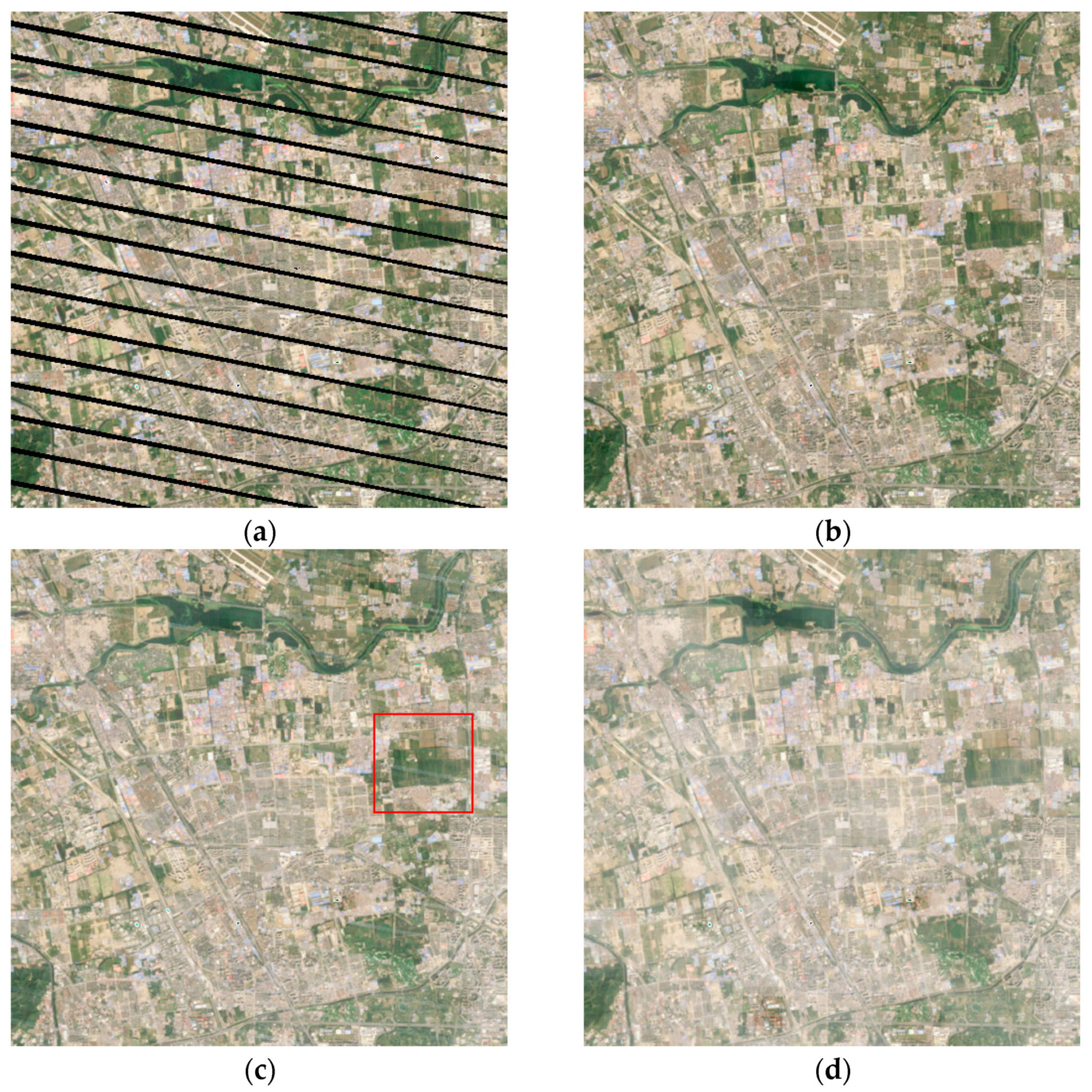
Situated in the northwest suburb of Beijing, the study region is located at approximately 40.10° N and 116.33° E, covered by World Reference System 2 Path 123 and Row 32. Within this Path/Row, we selected an intensive study area, which covers 15 km × 15 km (500 × 500 Landsat pixels). The land cover types include buildings, forests, grasslands, farmlands, roads, and rivers. Characterized by a temperate continental climate, the study region shows distinct seasons with significant vegetation changes. To clearly demonstrate the changes in the reconstructed time series, we selected a square (outlined in red in Figure 3c) to display the NDVI series.

For the present work, the Landsat SR dataset and the SDC500 [52] dataset are used to repair missing data and reconstruct dense time-series data. The Landsat SR dataset contains atmospherically corrected surface reflectance derived with the Landsat Ecosystem Disturbance Adaptive Processing System (LEDAPS) algorithm (version 3.4.0). For this dataset, we have chosen the blue, green, red, and near-infrared bands, each with a 30-meter spatial resolution and a 16-day temporal resolution (Landsat SR datasets are available for download at: https://earthexplorer.usgs.gov/, accessed on 9 April 2024). The Landsat 7 data used in this paper are clear images with less than 30% cloud cover and removed cloud and cloud shadows. All data have undergone preprocessing, including atmospheric correction, cloud removal, and cropping. Figure 1 illustrates the 25 Landsat 7 ETM+ images acquired between 2011 and 2013. The first 10 images correspond to acquisitions in 2011, and the subsequent 6 images pertain to the year 2012, and the final 9 images were acquired in 2013, with specific dates detailed in

Table 2. The date of the input images of Landsat images.

2011		2012	2013
7 January 2011	15 May 2011	26 January 2012	1 March 2013	4 November 2013
23 January 2011	20 September 2011	14 March 2012	18 April 2013	12 November 2013
31 January 2011	6 October 2011	30 March 2012	20 May 2013	28 November 2013
8 February 2011	23 November 2011	17 May 2012	1 September 2013	14 December 2013
28 March 2011	9 December 2011	21 August 2012	25 September 2013	30 December 2013
7 May 2011	25 December 2011	24 December 2012	11 October 2013

. All remote sensing images in the article are illustrated as true-color images of the red, green, and blue bands.

The global land surface reflectance Seamless Data Cube in 500 m resolution (SDC500) is also used in this study. Corresponding to MODIS-Terra sensor bands 1 to 7, this dataset reduces noise and fills gaps in the temporal reflectance series for each pixel. From this dataset, we have selected the blue, green, red, and near-infrared bands with a spatial resolution of 500 m and a temporal resolution of 1 day for the reconstruction process. (SDC500 dataset is available for download at: https://data-starcloud.pcl.ac.cn/resource/27/, accessed on 9 April 2024).

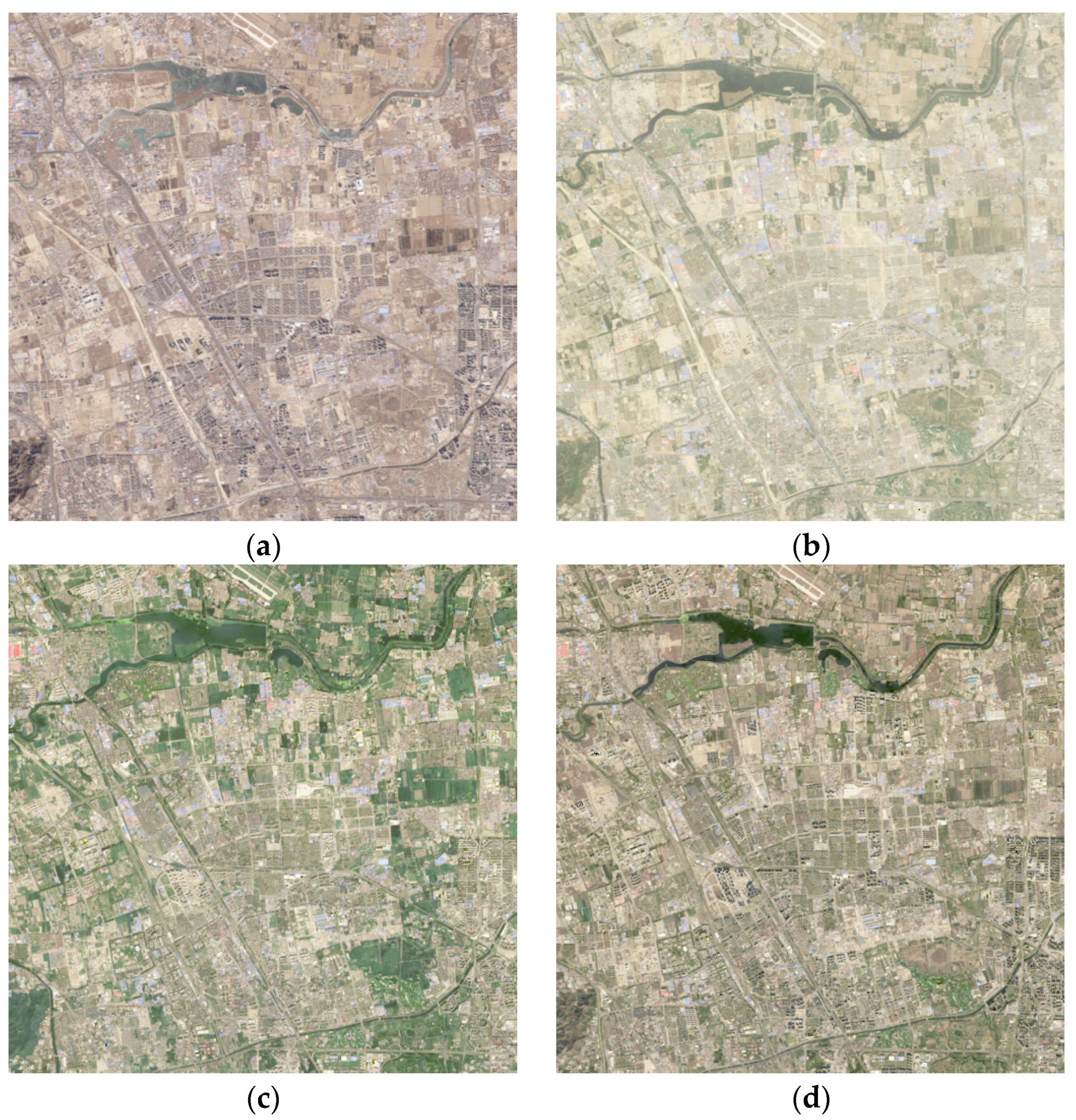
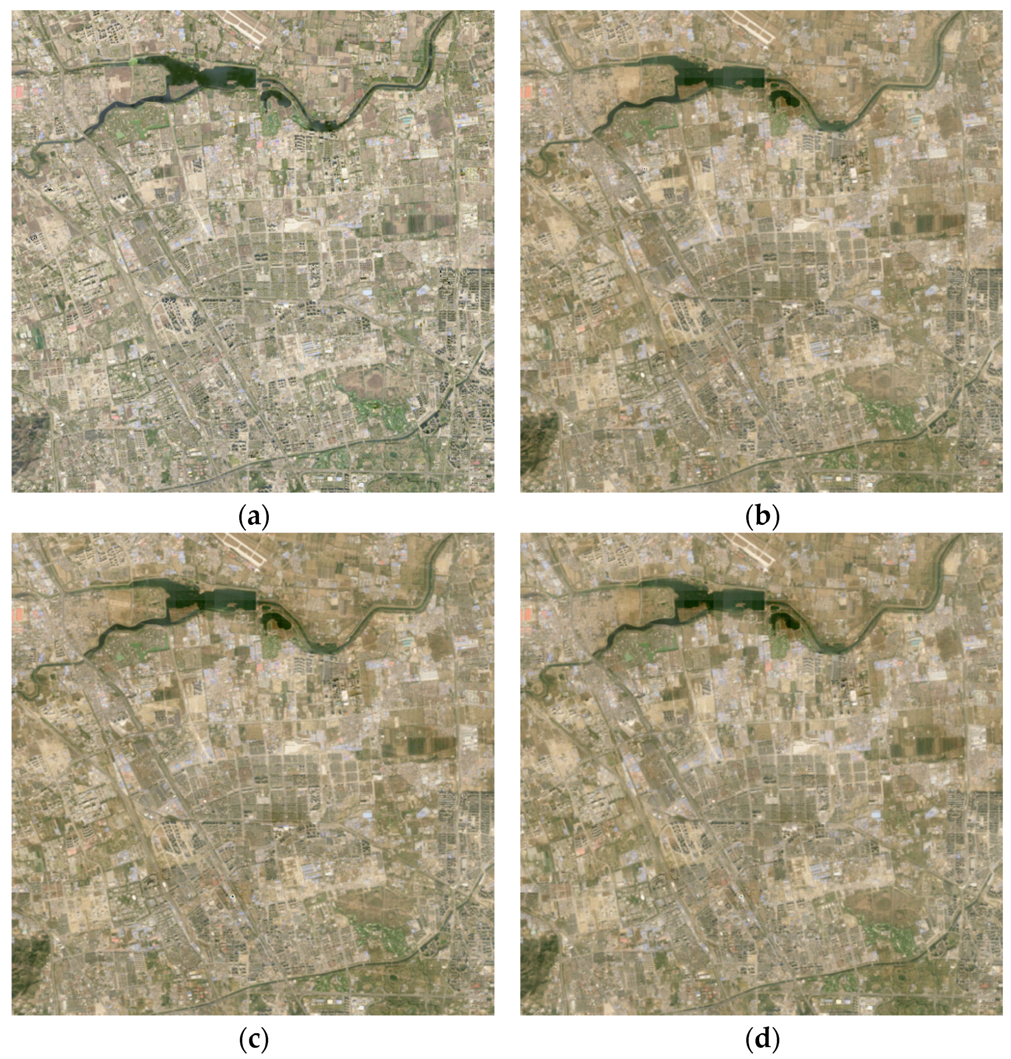
Figure 2 illustrates four images utilized for validation in this study, including Landsat 5 TM and Landsat 8 OLI images. The TM images were captured on 31 January 2011 (Figure 2a), and 7 May 2011 (Figure 2b), while the OLI images date from 1 September 2013 (Figure 2c), and 4 November 2013 (Figure 2d). These images distinctly illustrate significant surface reflectance changes in the region over a considerable time span. This region serves as an ideal area for testing algorithms with long temporal spans, as most existing methods face challenges in accurately reconstructing dense fine-resolution data over such extended periods.

3. Methodology

The ROBOT algorithm requires seamless data inputs, thereby necessitating interpolation preprocessing for SLC-off data. Aiming to reconstruct daily time-series images at a 30-meter resolution during the SLC-off period (especially around the year 2012), the IROBOT method can be viewed as an integration of the NSPI interpolation method and the ROBOT method.

3.1. The Neighborhood Similar Pixel (NSPI) Interpolation Method

Assuming that pixels with the same land cover class near data gaps have similar spectral characteristics and temporal change patterns as the missing target pixels, we can search for similar pixels near these gaps. Given a short time interval between the input and target scenes, we can select similar pixels from the input images and assume that these pixels also have similar spectral features with the missing target pixels on the target image [24]. Based on spectral similarity, Equation (1) defines the Root Mean Square Deviation (RMSD) between each common pixel and the target pixel, and we choose similar pixels based on these shared pixels.

$$RMS{D}_k=\sqrt{\frac{{\displaystyle \sum _{b=1}^N{\left(L(x_k,y_k,b)-L(x,y,b)\right)}^2}}{N}},$$

(1)

$L(x_k,y_k,b)$ represents the value of a common pixel in the input image at position $(x_k,y_k)$ in band $b$, and $L(x,y,b)$ represents the value in band $b$ at the target pixel $(x,y)$, $N$ is the number of spectral bands. A higher RMSD indicates greater spectral dissimilarity. Gao [28] utilized the standard deviation of the pixels in the input image and the estimated number of land cover types to determine the threshold. Pixels exhibiting RMSD values below this threshold are considered similar. This study employs built-in functions to automatically extract masks and categorize land cover types into pure pixels and others. If the RMSD of the k-th common pixel satisfies Equation (2), the k-th common pixel is chosen as a similar pixel.

$$RMS{D}_k\le {\displaystyle \sum _{b=1}^{nb}\sigma (b)}/N,$$

(2)

$\sigma (b)$ represents the standard deviation of the band $b$ across the entire input image. The parameters align with those in NSPI [24], where the initial search window is set to 7 × 7 pixels, and the minimum number of similar pixels is 30. When the initial window cannot contain the minimum number of similar pixels, the window expands until the minimum number of similar pixels is satisfied. However, to balance computational efficiency, the maximum window size is capped at 17 × 17 pixels. If the minimum number of similar pixels is not met when the window size reaches the maximum, all available similar pixels are used.

Higher spectral similarity and smaller distances of similar pixels should carry more weight when predicting the target pixel. The weight $W_j$ determines the contribution of the j-th similar pixel to the target pixel’s predicted value. Equation (3) calculates the geographic distance $D_j$ between the j-th similar pixel $(x_j,y_j)$ and the target pixel $(x,y)$. A comprehensive index $C{D}_j$ is outlined in Equation (4), which incorporated both spectral similarity (Equation (1)) and geographic distance.

$$D_j=\sqrt{{(x_j-x)}^2+{(y_j-y)}^2},$$

(3)

$$C{D}_j=RMS{D}_j\times D_j,$$

(4)

Similar pixels with larger $C{D}_j$ values contribute less to the calculated value of the target pixel. Therefore, we use the normalized reciprocal of $C{D}_j$ as the weight $W_j$ (as formulated in Equation (5)), where $W_j$ ranges from 0 to 1, ensuring that the cumulative weight of all similar pixels equals 1. Here, $NS$ is the number of similar pixels.

$$W_j=\left(1/C{D}_j\right)/{\displaystyle \sum _{j=1}^{NS}\left(1/C{D}_j\right)},$$

(5)

Since similar pixels have the same or similar spectral values to the target pixel during simultaneous observations, we can use the information from these similar pixels in the target image to predict the target pixel. A higher weight attributed to a similar pixel indicates greater reliability. Hence, the prediction of the target pixel is achieved by the weighted average of all similar pixels in the target image, as shown in Equation (6).

$$L_i(x,y)={\displaystyle \sum _{j=1}^{NS}{W}_j\times L_i(x_j,y_j)},$$

(6)

In instances where no similar pixel is selected, Inverse Distance Weighting (IDW) interpolation is employed to predict the target pixel’s value. This method gathers pixel values surrounding the target pixel, assigning higher weights to those closer to the target location. Following this interpolation process, the resulting seamless image is then ready for the subsequent phase of spatiotemporal fusion.

3.2. The ROBOT Algorithm

For coarse-resolution images, $C_i(i\in \{1,2,\dots ,n\})$ is the patch of the i-th input image pair represented as a flattened vector. There exists a sparse vector satisfying Equation (7):

$$C_p\approx D_C\alpha ,$$

(7)

where $D_C$ is stacked image patch vectors as matrices, $D_C=[C_1,C_2,\dots ,C_n]$, and $\alpha ={[{\alpha }_1,{\alpha }_2,\dots ,{\alpha }_n]}^T$ is a sparse vector, $n$ is the number of input images. We can find a compact and sparse representation as in Equation (7) by solving the LASSO (Least Absolute Shrinkage and Selection Operator) problem (Equation (8)), where $\lambda \in {\mathbb{R}}^{+}$ is a parameter.

$$\underset{\alpha }{\min }{\left|C_p-D_C\alpha \right|}_2^2+\lambda {\left|\alpha \right|}_1,$$

(8)

After obtaining the value of $\alpha$, in the same way, the estimation of the fine-resolution image can be expressed as Equation (9):

$${\widehat{F}}_p=D_F\alpha ,$$

(9)

where $D_F$ is stacked image patch vectors arranged as matrices, $D_F=[F_1,F_2,\dots ,F_n]$, $F_i(i\in \{1,2,\dots ,n\})$ is the fine-resolution image patch of the i-th input image pair as a flattened vector, ${\widehat{F}}_p$ is an estimation of the actual image $F_p$.

Variations in sensor specifications and observational perspectives can lead to inconsistencies between fine-resolution and coarse-resolution images, so the prediction in Equation (9) may contain noise. To mitigate this issue, a regularization term is introduced to enhance temporal correlation, and the optimized formula becomes:

$$\underset{\alpha }{\min }{\left|C_p-D_C\alpha \right|}_2^2+\lambda {\left|\alpha \right|}_1+\beta \left({\left|F_{nearest}-D_F\alpha \right|}_2^2\right),$$

(10)

$$F_{nearest}=\frac{F_i+F_{i+1}}{2},T_p\in [T_i,T_{i+1}].$$

(11)

Here, $F_{nearest}$ represents the fine-resolution image closest to the predicted moment in time, $T_i$ is a time flag of the i-th input image pair, $T_p$ is the time flag of the prediction phase, $\beta \in {\mathbb{R}}^{+}$ is a parameter.

Considering the presence of approximate residual $\Delta C$ in coarse-resolution images (as depicted in Equation (12)), it is necessary to distribute the residuals into the prediction of fine resolution represented by sparse vectors. These residuals are then integrated into the final prediction, as formulated in Equation (13).

$$\Delta C=C_p-D_C\alpha ,$$

(12)

$${\widehat{F}}_p=C_p+\left(D_F-D_C\right)\alpha ,$$

(13)

3.3. The Improved ROBOT (IROBOT) Algorithm

In the ROBOT algorithm, a high-quality reference image $F_{nearest}$ (represented by Equation (11)) is required as the average image around $T_p$. This approach stabilizes the output during the reconstruction of time-series images. However, mosaic artifacts may emerge in the reconstructed images if the input images are of poor quality or are limited in quantity. To address this, we modify $F_{nearest}$ to be a piecewise function as shown in Equation (14):

$$F_{nearest}=\{\begin{array}{c}{F}_i,T_P\in \left(T_i,\delta \right)\\ \frac{F_{i+1}+F_i}{2},T_p\notin \left(T_i,\delta \right)\end{array}.$$

(14)

When predicting the image at time point $p$ within the time neighborhood $\left(T_i,\delta \right)$, the predicted image should be more similar to the i-th input image than the average of adjacent images. The L1 norm constraint controlled by the parameter $\lambda$ compresses data and reduces model complexity. The L2 norm constraint controlled by parameter $\beta$ preserves most features of $F_i$ and generates a stable predicted image.

Additionally, when the available quantity of images is less, we handle $\beta$ differently. If the time flag of the predicted image is not closely aligned with the input image time series, indicating significant temporal differences between the predicted image and $F_i$, the spatial structure of the predicted image relative to $F_i$ may change. In such cases, it is advisable to relinquish the L2 norm constraint and employ the L1 norm constraint only. This allows for the automatic selection of the most crucial features in datasets with abundant features, generating a fine-resolution predicted image that aligns with the selected features. We devised a strategy to abandon the L2 norm constraint when the number of available images is less than 7; the parameters are set to $\lambda =1,\beta =0$.

3.4. Experimental Design

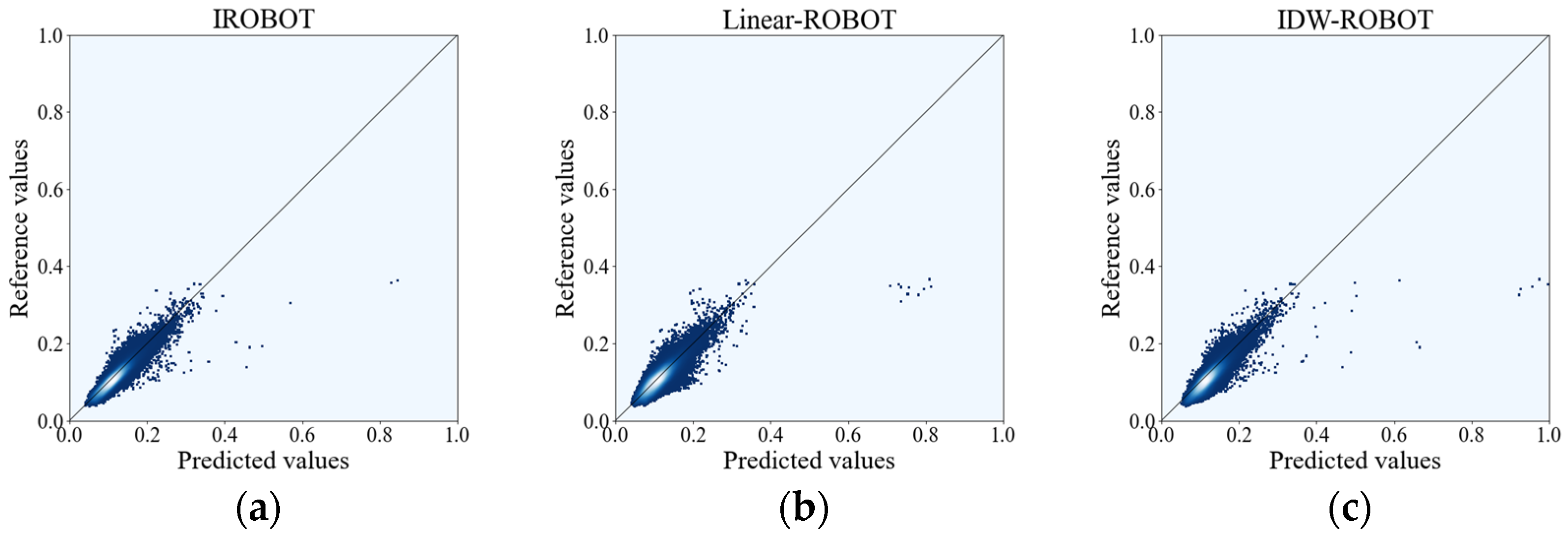
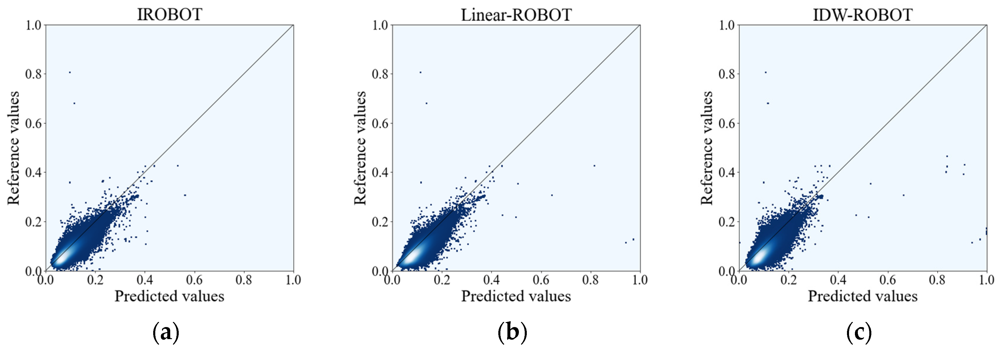
Interpolating SLC-off data is a crucial step in reconstructing dense time series using the ROBOT algorithm. In our experiments, we primarily focused on comparing the effects of different interpolation methods on the reconstruction results. Specifically, we integrated two distinct interpolation techniques with the original ROBOT algorithm to serve as comparative algorithms. The Linear-ROBOT method identifies valid pixels before and after the target image’s date, employing time-based linear interpolation to fill the invalid striped pixels, before applying the original ROBOT algorithm [49] for reconstructing complete annual time-series data. Conversely, the IDW-ROBOT method adopts inverse distance weighted interpolation for filling in missing values prior to the reconstruction process with the original ROBOT algorithm [49]. Both comparison methods use the same input images as IROBOT. This article designed three experiments: Experiment I and Experiment II were conducted to demonstrate the reconstruction effect, while Experiment III was performed to analyze the continuity of reconstructed time-series images. Each experiment presented the results of the proposed IROBOT method as well as those of the comparative methods.

Experiment I involves the recovery and reconstruction of Landsat 7 SLC-off data in 2011 (images shown in Figure 1). The input data for the IROBOT method consisted of SLC-off data (fine images) and SDC data (coarse images) from 2011, and the parameters are set to $\lambda =2,\beta =1,\delta =24$. Clear Landsat 5 TM images, as shown in Figure 2a,b, are selected as the reference images for a quantitative evaluation of the reconstruction in the blue, green, red, and near-infrared (NIR) bands. The TM sensor can be regarded as a homologous sensor compared to the ETM+ sensor [53], so in this experiment, the reconstructed image can be directly compared to the reference image without the need for sensor transformation.

Experiment Ⅱ encompasses the restoration and reconstruction of Landsat 7 SLC-off data captured in 2013. During this year, the Landsat 8 satellite could provide high-quality images as a reference. Considering the sensor disparities between ETM+ and OLI, the Landsat 7 reflectance data can be linearly transformed following the approach outlined by Roy [53,54] to ensure consistency between the images captured by the two sensors. The regression coefficients for the transformation from ETM+ to OLI are provided in

Table 3. Surface reflectance sensor transformation functions (ETM+ to OLI) derived by ordinary least squares (OLS) regression and reduced major axis (RMA) regression coefficients.

Band	Regression Type	Between Sensors OLS and RMA Transformation Functions
Blue	OLS	OLI = 0.0003 + 0.8474 ETM+
	RMA	OLI = −0.0095 + 0.9785 ETM
Green	OLS	OLI = 0.0088 + 0.8483 ETM+
	RMA	OLI = −0.0016 + 0.9542 ETM
Red	OLS	OLI = 0.0061 + 0.9047 ETM+
	RMA	OLI = −0.0022 + 0.9825 ETM
NIR	OLS	OLI = 0.0412 + 0.8462 ETM+
	RMA	OLI = −0.0021 + 1.0073 ETM

. The formula for converting the surface reflectance data from ETM+ to OLI, incorporating the scaling factors from the SR dataset, is given by Equation (15). The 9 Landsat 7 ETM+ images of 2013 in Figure 1 are transformed into OLI images via RMA regression. So, the fine-resolution images are the converted Landsat 7 OLI images, and coarse-resolution images are SDC images of the year 2013. These input images are utilized for the reconstruction process, aligning with the procedures outlined in Experiment I. The clear Landsat 8 images are selected as the reference images (as shown in Figure 2c,d), and the restoration reconstruction results of the two methods on four bands are evaluated.

$$S{R}_{OLI}=S{R}_{ETM+}\times Slopes+\frac{Offset(Slopes-1)+Itcps}{Scale}.$$

(15)

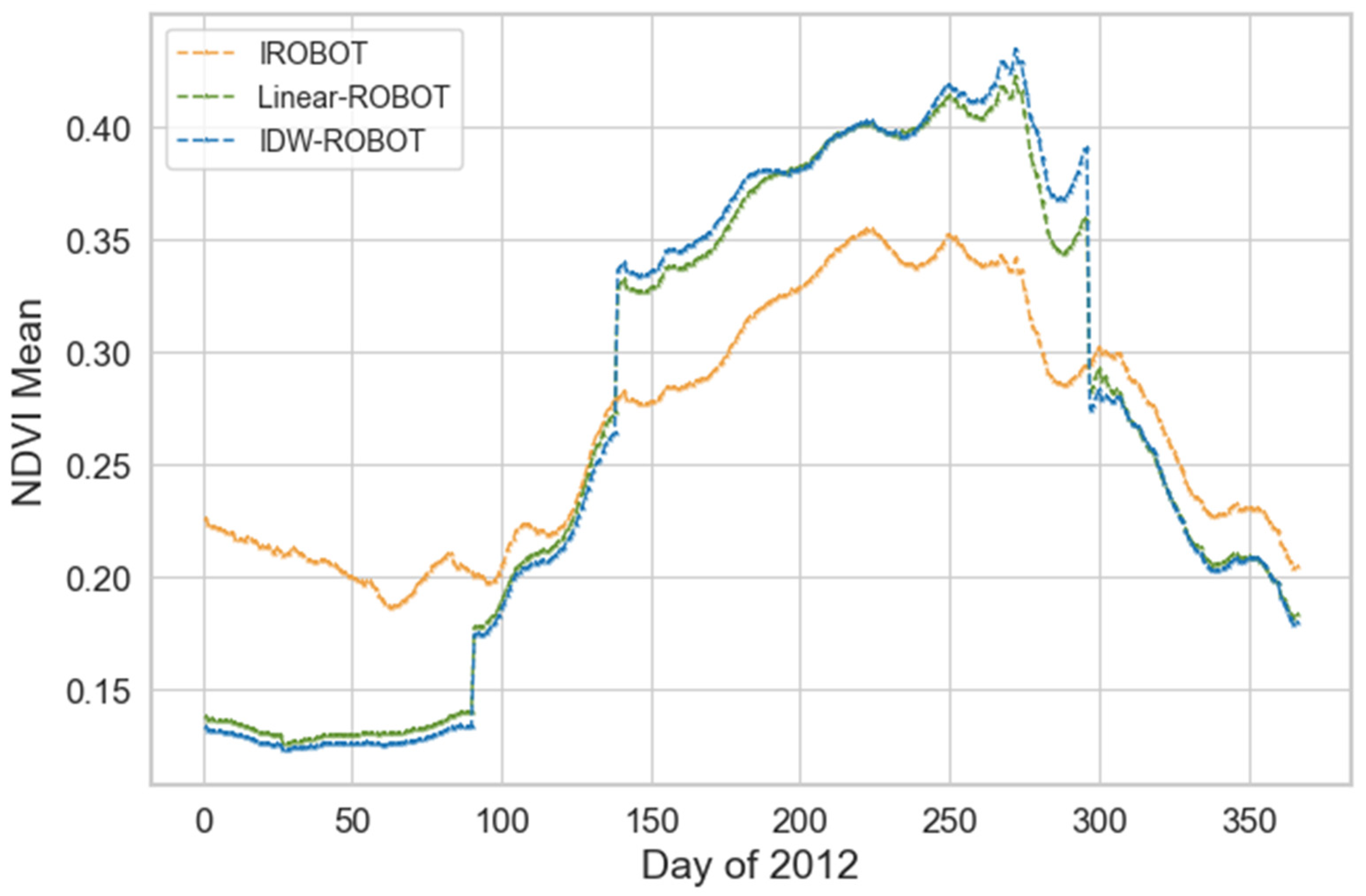
Experiment Ⅲ is to reconstruct the daily Landsat 7 reflectance data for 2012. Due to the limited availability of Landsat 7 images in 2012, comprising only 6 images, we devised a strategy to abandon the parameter $\beta$ when the number of available images is less than 7. To enhance feature availability, the temporal input range is extended to include four additional months around 2012, thus incorporating 5 images from August to December 2011 and 2 from January to April 2013. In this experiment, we reconstructed the time-series data using IROBOT, Linear-ROBOT, and IDW-ROBOT methods, and all algorithms used 13 Landsat images as input for fine-resolution data (including 7 images from 2011 and 2013) and SDC500 images in 2012 for coarse-resolution data. Moreover, the NDVI time series of the reconstructed results are calculated and represented by a line chart.

3.5. Evaluation Metrics

In terms of qualitative assessment, visual inspection of the reconstructed images is conducted to assess their spatial continuity. Additionally, scatter plots comparing reconstructed images with reference images are used for qualitative evaluation of the reconstruction results. Regarding quantitative assessment, the Mean Absolute Error (MAE), BIAS, Correlation Coefficient (CC), and Structural Similarity Index Metric (SSIM) are employed to compare the reconstructed image with reference image data. When the values of MAE and BIAS are close to 0, and the values of CC and SSIM are close to 1, it indicates superior performance in predicting image quality.

4. Results and Analysis

This article presents three experiments to demonstrate the effectiveness of the proposed method in repairing SLC-off data (the results of the simulated gap images are shown in the Supplementary Materials). Experiment I and Experiment II used TM images and OLI images as references to verify the reconstructed images, Experiment III shows the partial reconstructed images in 2012 and compares the continuity of the NDVI time series reconstructed by the IROBOT, Linear-ROBOT, and IDW-ROBOT methods. Subsequently, the study analyzes the impact of the number of input images and the sensor conversion coefficient on the reconstruction results.

4.1. Experiment I: Evaluation of the Reconstruction Results with Landsat 5 Images

Experiment I reconstructs seamless 30-m resolution images for the year 2011 using Landsat 7 SLC-off data and SDC500 data from 2011. The image of 20 September 2011 is taken as an example for visual inspection (the images of input images before and after gap-filling are shown in Figure A1). Figure 3b–d represent the results of the reconstruction of the input image (Figure 3a) using the IROBOT, Linear-ROBOT, and IDW-ROBOT methods, respectively. It can be seen that the reconstructed images of the three methods are similar to the input image (Figure 3a), with the gap basically repaired. However, shallow traces can be observed on the red square of Figure 3c, and the color of Figure 3d appears lighter. In comparison, Figure 3b exhibits spatial continuity without gaps and is more similar to the input image (Figure 3a) compared to the other methods.

We quantified the MAE, BIAS, CC, and SSIM to compare the reconstructed images from the three methods. Figure 4 shows the reference image (Figure 4a) and reconstructed images (Figure 4b–d).

Table 4. The accuracy of three methods on 31 January 2011.

Evaluation Metrics	IROBOT				Linear-ROBOT				IDW-ROBOT
	Blue	Green	Red	NIR	Blue	Green	Red	NIR	Blue	Green	Red	NIR
MAE	0.0069	0.0108	0.0090	0.0098	0.0110	0.0196	0.0176	0.0175	0.0104	0.0168	0.0141	0.0119
BIAS	0.0014	0.0093	0.0052	0.0023	0.0091	0.0189	0.0161	0.0151	0.0081	0.0160	0.0122	0.0040
CC	0.9288	0.9429	0.9543	0.9617	0.9127	0.9213	0.9282	0.9445	0.9110	0.9274	0.9410	0.9480
SSIM	0.9363	0.9441	0.9499	0.9407	0.9157	0.9129	0.9186	0.9161	0.9197	0.9231	0.9312	0.9210

presents the accuracy of the reconstructed images by the three methods in comparison to the reference image on 31 January. The CC and SSIM values for all methods are comparably high, exceeding 0.9. The MAE and BIAS of the IROBOT method are closer to 0 than those of the other two methods. The MAE and BIAS are the minimum ones compared to the other two methods. Notably, in the blue band, the IROBOT method achieves the lowest MAE (0.0069) and BIAS (0.0014) among the methods. The scatter plot in Figure 5 shows the relationship between the predicted values and the reference values for the blue band. It can be clearly seen that the data points in the scatter plot of the IROBOT method (Figure 5a) are closer to the 1:1 line than those of the Linear-ROBOT method (Figure 5b) and the IDW-ROBOT method (Figure 5c). Table 4 and Figure 5 indicate that the IROBOT method can reconstruct the image relatively accurately, even when the input image’s acquisition date significantly deviates from that of the reconstructed image.

Surface reflectance in the images from 7 May (Figure 6a) exhibited significant changes compared to those from 31 January (Figure 4a).

Table 5. The accuracy of three methods on 7 May 2011.

Evaluation Metrics	IROBOT				Linear-ROBOT				IDW-ROBOT
	Blue	Green	Red	NIR	Blue	Green	Red	NIR	Blue	Green	Red	NIR
MAE	0.0089	0.0082	0.0126	0.0156	0.0106	0.0121	0.0153	0.0277	0.0145	0.0121	0.0181	0.0163
BIAS	0.0063	0.0026	0.0096	0.0124	0.0038	−0.0048	−0.0074	0.0239	0.0131	0.0088	0.0164	0.0122
CC	0.9209	0.9177	0.9186	0.9334	0.8659	0.8689	0.8699	0.8102	0.8863	0.8981	0.9081	0.9139
SSIM	0.9796	0.9763	0.9664	0.9599	0.9670	0.9575	0.9409	0.8966	0.9692	0.9691	0.9563	0.9526

provides a quantitative assessment of the reconstruction accuracy of the three methods against the reference image (Figure 6a). The IROBOT method generally shows smaller MAE and BIAS, along with higher CC and SSIM values, except for a slightly higher BIAS in the blue band compared to the Linear-ROBOT method. For all bands, the IROBOT method’s CC and SSIM values exceed 0.90 and 0.95, respectively. Notably, in the NIR band, the IROBOT method demonstrates substantial improvement, with increases of 0.1232 in CC and 0.0633 in SSIM (IROBOT: CC 0.9334, SSIM 0.9599; Linear-ROBOT: CC 0.8102, SSIM 0.8966). The scatter plot (Figure 7a) for the IROBOT method shows data points more closely aligned with the 1:1 line compared to those in Figure 7b,c, indicating that the IROBOT method estimates the predicted values with higher accuracy.

Liu [50] proposed a method that utilized the NSPI [24] and ESTARFM [30] algorithms to fill in missing values and construct time-series data. As a comparison, we present the reconstructed images of this “NSPI + ESTARFM” method from 31 January and 7 May (Figure A3) using this method, as well as the accuracy metrics compared to the reference images (

Table A1. The accuracy of images reconstructed using the NSPI + ESTARFM method.

Evaluation Metrics	31 January 2011				7 May 2011
	Blue	Green	Red	NIR	Blue	Green	Red	NIR
MAE	0.0110	0.0195	0.0161	0.0122	0.0095	0.0135	0.0103	0.0198
BIAS	0.0097	0.0192	0.0152	0.0075	0.0082	0.0124	0.0055	0.0170
CC	0.9196	0.9364	0.9491	0.9553	0.9284	0.9225	0.9113	0.8860
SSIM	0.9281	0.9301	0.9401	0.9318	0.9765	0.9695	0.9618	0.9412

) in Appendix B. The accuracy table shows that overall, the quality metrics of the reconstructed images obtained using this method are inferior to those of the IROBOT algorithm. This is because the fusion effectiveness of the ESTARFM algorithm is not as good as that of the ROBOT algorithm. The ESTARFM algorithm relies on two high-quality fine-resolution images, which are often not available, to predict the image at a specific time, whereas the ROBOT algorithm uses the multi-resolution time-series data to predict the image at a specific time, significantly improving the accuracy of the predicted images. Furthermore, the ESTARFM method is not suitable for processing large remote sensing datasets as its computational efficiency is significantly lower than that of the ROBOT algorithm.

4.2. Experiment II: Evaluation of the Reconstruction Results with Landsat 8 Images

The TM sensor and ETM+ sensor are often considered homologous sensors. Experiment I demonstrates that the IROBOT method achieves good reconstruction results with homologous sensor data, but the transformation between different sensors does not affect the advantages of the IROBOT method. Experiment Ⅱ reconstructs seamless 30-m resolution images for 2013 using SLC-off data transformed by RMA and SDC500 data. It uses the transformed gap images and Landsat 8 OLI images as reference images to evaluate the reconstruction effectiveness of the IROBOT method and contrasting methods on the corresponding dates of the reference images.

A visual inspection conducted on the images from 25 September 2013 reveals distinct outcomes. Figure 8b–d display the reconstruction results for this date using the IROBOT, Linear-ROBOT, and IDW-ROBOT methods, respectively. The IROBOT method’s reconstructed image (Figure 8b) is very similar to the input image (Figure 8a) with gaps well repaired. However, gap traces are noticeable in the Linear-ROBOT method’s output (Figure 8c), and both Figure 8c,d have significant color differences with the input image. The images of transformed images before and after gap-filling are shown in Figure A2. Overall, the IROBOT method produces a result that is more similar to the input image compared to the other methods.

Taking the Landsat 8 OLI image on 1 September 2013 (Figure 9a) as the reference, the image (Figure 9b) reconstructed by the IROBOT method is more spatially continuous and clearer. In contrast, the Linear-ROBOT reconstruction (Figure 9c) shows obvious strips, and the IDW-ROBOT reconstruction (Figure 9d) appears slightly blurred.

Table 6. The accuracy of three methods on 1 September 2013.

Evaluation Metrics	IROBOT				Linear-ROBOT				IDW-ROBOT
	Blue	Green	Red	NIR	Blue	Green	Red	NIR	Blue	Green	Red	NIR
MAE	0.0190	0.0235	0.0299	0.0294	0.0257	0.0309	0.0398	0.0313	0.0268	0.0325	0.0406	0.0367
BIAS	0.0160	0.0215	0.0279	0.0157	0.0245	0.0300	0.0389	0.0141	0.0250	0.0310	0.0390	0.0243
CC	0.8306	0.8370	0.8643	0.8584	0.8064	0.8104	0.8289	0.8328	0.7917	0.7932	0.8326	0.8194
SSIM	0.9018	0.9301	0.8980	0.8584	0.8718	0.9089	0.8622	0.8469	0.8629	0.9003	0.8552	0.8239

shows MAE, BIAS, CC, and SSIM values for the reference image and reconstructed Landsat 7 OLI images. The IROBOT method demonstrates superior overall accuracy, despite the Linear-ROBOT method having a marginally lower BIAS value in the NIR band (IROBOT: 0.0157, Linear-ROBOT: 0.0141). The scatter plots in Figure 10a–c show the relationship between the reconstructed images of the three methods and the reference image for the blue band. The data points in the scatter plot of the IROBOT method are more concentrated around the 1:1 line, indicating that the predictions of this method are more accurate.

Compared to Figure 9a, Figure 11d highlights a two-month time span during which there is a significant change in surface reflectance. While the images reconstructed by the three methods are very similar, the reconstruction accuracy (as presented in

Table 7. The accuracy of three methods on 4 November 2013.

Evaluation Metrics	IROBOT				Linear-ROBOT				IDW-ROBOT
	Blue	Green	Red	NIR	Blue	Green	Red	NIR	Blue	Green	Red	NIR
MAE	0.0132	0.0123	0.0115	0.0183	0.0158	0.0145	0.0133	0.0186	0.0170	0.0158	0.0149	0.0198
BIAS	−0.0114	−0.0102	−0.0067	0.0145	−0.0146	−0.0132	−0.0100	0.0140	−0.0159	−0.0145	−0.0117	0.0143
CC	0.9031	0.9246	0.9345	0.9377	0.8961	0.9202	0.9300	0.9314	0.8877	0.9105	0.9214	0.9203
SSIM	0.9035	0.9215	0.9235	0.9315	0.8836	0.9126	0.9161	0.9277	0.8633	0.8922	0.8961	0.9096

) of Figure 11b is obviously better. The IROBOT method exhibits slightly smaller MAE and BIAS values, along with higher CC and SSIM values. In the scatter plots of Figure 12, the IROBOT method’s data points align more closely with the 1:1 line, suggesting that its estimated values are more precise compared to the other methods.

4.3. Experiment III: Reconstruction of the Dense and Continuous Time-Series NDVI

The previous two experiments show that the proposed method can reconstruct more reliable time-series data, which can be used for subsequent application research. In the third experiment, high spatial resolution SLC-off images from October 2011 to April 2013, along with high temporal resolution SDC500 data for 2012, served as input. A time series of daily seamless 30-m data for the year 2012 is reconstructed using these data. Due to space constraints, only the images from the 1st day of each month are displayed in Figure 13. It can be observed that the IDW-ROBOT method’s reconstructed images appear incomplete for April and May, whereas the IROBOT and Linear-ROBOT methods’ images exhibit dynamic changes corresponding to the seasonal transitions.

For an in-depth investigation into the continuity in temporal dimension, the daily NDVI profile is extracted at some typical vegetation pixels in the study region. Figure 14 illustrates the NDVI time series reconstructed using three methods within the red-line square of Figure 3c. The time series reconstructed by the Linear-ROBOT and IDW-ROBOT methods exhibit noticeable abrupt changes (at approximately points 50, 100, and 300 on the horizontal axis), which are primarily attributed to the influence of parameter $\beta$. In contrast, the NDVI mean curve reconstructed by the IROBOT method demonstrates greater continuity throughout the observed period.

4.4. Temporal Continuity Analysis with Varying Numbers of Input Images

Given the limited number of available images, existing spatiotemporal fusion methods [27,28,29,30,31,32,33,34,35,36,37,38,39,40,41,42,43,44,45,46,47,48,49,50] fall short in reconstructing dense time-series data. This inadequacy stems primarily from two factors: firstly, the current spatiotemporal fusion methods rely heavily on changes between two coarse-resolution images, limiting the precision in predicting fine-resolution images. Secondly, traditional fusion methods are time-intensive and ill-suited for processing large-scale datasets. The ROBOT algorithm, however, efficiently harnesses the available information within the time series. As noted by Chen [49], an increased number of input images enhances the reconstruction outcome, a principle that should extend to SLC-off data as well.

Only six SLC-off images were available in 2012. This section uses these six images as fine-resolution input data to reconstruct the 2012 dense time-series images. The reconstruction outcomes are then compared with those from Experiment III, which utilized 13 images as fine-resolution input data. Figure 15 illustrates the reconstructed images on the 100th day of 2012. Figure 15a has a slight mosaic phenomenon, while Figure 15b is relatively better using more input images. Therefore, the expansion of time-series images is helpful for us to obtain enough image features and maintain clear reconstruction results. Thus, expanding the time-series images proves beneficial in acquiring sufficient image features and achieving clearer reconstruction results.

4.5. Comparative Analysis of the Reconstruction Results Using RMA and OLS Regression Coefficients

Joy [53] proposed surface reflectance sensor transformation functions derived by reduced major axis (RMA) regression and ordinary least squares (OLS) regression. RMA regression is more sensitive to the relationship between variables in data samples containing errors; therefore, it is especially suitable for the study of the conversion coefficient between different sensors. Although RMA regression coefficients are frequently employed for sensor conversion [55,56], comparisons between RMA and OLS regression coefficients are scarce. In Section 4.2, we utilized the RMA transformation function to reconstruct time-series images for 2013. Conversely, this section employs Landsat 7 data transformed using the OLS regression function for reflectance data reconstruction, facilitating a comparative analysis with the results from Section 4.2.

The discrepancies between images reconstructed by the two regression functions are small, with closely aligned evaluation metrics. Comparing Table 6 and

Table 8. The accuracy of three methods (via OLS regression) on 7 May 2013.

Evaluation Metrics	IROBOT				Linear-ROBOT				IDW-ROBOT
	Blue	Green	Red	NIR	Blue	Green	Red	NIR	Blue	Green	Red	NIR
MAE	0.0183	0.0226	0.0287	0.0352	0.0247	0.0298	0.0384	0.0375	0.0262	0.0318	0.0396	0.0436
BIAS	0.0147	0.0200	0.0262	0.0243	0.0230	0.0286	0.0372	0.0246	0.0240	0.0300	0.0378	0.0338
CC	0.8173	0.8259	0.8604	0.8485	0.7942	0.8010	0.8263	0.8219	0.7806	0.7857	0.8331	0.8071
SSIM	0.9012	0.9304	0.8975	0.8357	0.8727	0.9100	0.8631	0.8257	0.8580	0.8981	0.8532	0.7992

, the reconstructed images on 7 May show that the MAE and BIAS values with RMA regression are greater than those with OLS regression (except for the NIR band), where CC and SSIM values are nearer to 1. Furthermore, the comparison between Table 7 and

Table 9. The accuracy of three methods (via OLS regression) on 4 November 2013.

Evaluation Metrics	IROBOT				Linear-ROBOT				IDW-ROBOT
	Blue	Green	Red	NIR	Blue	Green	Red	NIR	Blue	Green	Red	NIR
MAE	0.0142	0.0129	0.0124	0.0160	0.0150	0.0135	0.0128	0.0165	0.0159	0.0146	0.0141	0.0178
BIAS	−0.0126	−0.0108	−0.0076	0.0007	−0.0136	−0.0116	−0.0086	0.0021	−0.0146	−0.0126	−0.0099	0.0019
CC	0.9017	0.9232	0.9341	0.9338	0.8931	0.9181	0.9295	0.9288	0.8850	0.9090	0.9214	0.9178
SSIM	0.8889	0.9069	0.9130	0.9087	0.8846	0.9057	0.9115	0.9084	0.8657	0.8852	0.8912	0.8887

shows that images reconstructed via RMA regression exhibit smaller MAE and BIAS, and higher CC and SSIM values in the blue, green, and red bands. The observed trends suggest that RMA regression is preferable to OLS regression, especially when dealing with data containing errors beyond the researchers’ control.

5. Conclusions

In this paper, a Seamless Data Cube reconstruction method named IROBOT is proposed to fill missing values in the Landsat 7 SLC-off images and reconstruct spatially complete and dense time-series data. It inherits most of the advantages of the ROBOT algorithm, featuring high computational efficiency, infrequent parameter adjustments, and adaptability to various data structures without process customization. With an equal number of input images, this method outperforms existing SLC-off reconstruction methods in terms of temporal resolution, and the reconstructed result is superior to the original ROBOT method. The IROBOT method was also more stable when the number of input images was less. Overall, it holds significant promise for providing high-quality analysis-ready images around year 2012 from Landsat 7 SLC-off data, and serves as an algorithm component in the project to build a global and long-term continuous 30 m resolution SDC to facilitate research on global change and land surface dynamics.

References

1. Wulder, M.A.; Loveland, T.R.; Roy, D.P.; Crawford, C.J.; Masek, J.G.; Woodcock, C.E.; Allen, R.G.; Anderson, M.C.; Belward, A.S.; Cohen, W.B.; et al. Current status of Landsat program, science, and applications. Remote Sens. Environ. 2019, 225, 127–147. [Google Scholar] [CrossRef]
2. Roy, D.P.; Ju, J.; Kline, K.; Scaramuzza, P.L.; Kovalskyy, V.; Hansen, M.; Loveland, T.R.; Vermote, E.; Zhang, C. Web-enabled Landsat Data (WELD): Landsat ETM+ composited mosaics of the conterminous United States. Remote Sens. Environ. 2010, 114, 35–49. [Google Scholar] [CrossRef]
3. Loveland, T.R.; Dwyer, J.L. Landsat: Building a strong future. Remote Sens. Environ. 2012, 122, 22–29. [Google Scholar] [CrossRef]
4. Wulder, M.A.; Masek, J.G.; Cohen, W.B.; Loveland, T.R.; Woodcock, C.E. Opening the archive: How free data has enabled the science and monitoring promise of Landsat. Remote Sens. Environ. 2012, 122, 2–10. [Google Scholar] [CrossRef]
5. Suliman, S.I. Locally Linear Manifold Model for Gap-Filling Algorithms of Hyperspectral Imagery: Proposed Algorithms and a Comparative Study. Master’s Thesis, Michigan State University, East Lansing, MI, USA, 2016. [Google Scholar]
6. Maxwell, S.K.; Schmidt, G.L.; Storey, J.C. A multi-scale segmentation approach to filling gaps in Landsat ETM+ SLC-off images. Int. J. Remote Sens. 2007, 28, 5339–5356. [Google Scholar] [CrossRef]
7. United States Geological Survey (USGS). Preliminary Assessment of Landsat 7 ETM+ Data following Scan Line Corrector Malfunction. Available online: https://www.usgs.gov/media/files/preliminary-assessment-value-landsat-7-etm-slc-data.pdf (accessed on 20 December 2018).
8. Wulder, M.A.; Coops, N.C.; Roy, D.P.; White, J.C.; Hermosilla, T. Land cover 2.0. Int. J. Remote Sens. 2018, 39, 4254–4284. [Google Scholar] [CrossRef]
9. Graesser, J.; Stanimirova, R.; Friedl, M.A. Reconstruction of Satellite Time Series With a Dynamic Smoother. IEEE J. Sel. Top. Appl. Earth Obs. Remote Sens. 2022, 15, 1803–1813. [Google Scholar] [CrossRef]
10. Farhat, L.; Manakos, I.; Sylaios, G.; Kalaitzidis, C. A Modified Version of the Direct Sampling Method for Filling Gaps in Landsat 7 and Sentinel 2 Satellite Imagery in the Coastal Area of Rhone River. Remote Sens. 2023, 15, 5122. [Google Scholar] [CrossRef]
11. Case, N.; Vitti, A. Reconstruction of Multi-Temporal Satellite Imagery by Coupling Variational Segmentation and Radiometric Analysis. ISPRS Int. J. Geo-Inf. 2021, 10, 17. [Google Scholar] [CrossRef]
12. Ali, S.M.; Mohammed, M.J. Gap-Filling Restoration Methods for ETM+ Sensor Images. Iraqi J. Sci. 2013, 54, 206–214. [Google Scholar]
13. Olivier, R.; Hanqiang, C. Nearest Neighbor Value Interpolation. Int. J. Adv. Comput. Sci. Appl. (IJACSA) 2012, 3, 25–30. [Google Scholar] [CrossRef]
14. Wang, H.; Zhou, L.; Zhang, J. A region-based bi-cubic image interpolation algorithm. Comput. Eng. 2010, 36, 216–218. [Google Scholar]
15. Zhang, C.; Li, W.; Travis, D. Gaps-fill of SLC-off Landsat ETM plus satellite image using a geostatistical approach. Int. J. Remote Sens. 2007, 28, 5103–5122. [Google Scholar] [CrossRef]
16. Pringle, M.J.; Schmidt, M.; Muir, J.S. Geostatistical interpolation of SLC-off Landsat ETM+ images. ISPRS J. Photogramm. Remote Sens. 2009, 64, 654–664. [Google Scholar] [CrossRef]
17. Boloorani, A.D.; Erasmi, S.; Kappas, M. Multi-Source Remotely Sensed Data Combination: Projection Transformation Gap-Fill Procedure. Sensors 2008, 8, 4429–4440. [Google Scholar] [CrossRef]
18. Zhu, X.; Liu, D.; Chen, J. A new geostatistical approach for filling gaps in Landsat ETM+ SLC-off images. Remote Sens. Environ. 2012, 124, 49–60. [Google Scholar] [CrossRef]
19. Zeng, C.; Shen, H.; Zhang, L. Recovering missing pixels for Landsat ETM+ SLC-off imagery using multi-temporal regression analysis and a regularization method. Remote Sens. Environ. 2013, 131, 182–194. [Google Scholar] [CrossRef]
20. Maxwell, S.K. Filling Landsat ETM+ SLC-off gaps using a segmentation model approach. Photogramm. Eng. Remote Sens. 2004, 70, 1109–1111. [Google Scholar]
21. Marujo, R.F.B.; Fonseca, L.M.G.; Körting, T.S.; Bendini, H.N. A multi-scale segmentation approach to filling gaps in landsat ETM+ SLC-off images through pixel weighting. Int. Arch. Photogramm. Remote Sens. Spat. Inf. Sci. 2020, XLII-3, 79–84. [Google Scholar] [CrossRef]
22. SLC Gap-Filled Products Phase One Methodology. Available online: https://www.usgs.gov/media/files/landsat-7-slc-gap-filled-products-phase-one-methodology (accessed on 2 August 2019).
23. Phase 2 Gap-Fill Algorithm: SLC-Off Gap-Filled Products Gap-Filled Algorithm Methodology. Available online: https://www.usgs.gov/media/files/landsat-7-slc-gap-filled-products-phase-two-methodology (accessed on 20 December 2018).
24. Chen, J.; Zhu, X.; Vogelmann, J.E.; Gao, F.; Jin, S. A simple and effective method for filling gaps in Landsat ETM+ SLC-off images. Remote Sens. Environ. 2011, 115, 1053–1064. [Google Scholar] [CrossRef]
25. Zhu, X.; Gao, F.; Liu, D.; Chen, J. Modified Neighborhood Similar Pixel Interpolator Approach for Removing Thick Clouds in Landsat Images. IEEE Geosci. Remote Sens. Lett. 2012, 9, 521–525. [Google Scholar] [CrossRef]
26. Liu, H.; Gong, P.; Wang, J.; Wang, X.; Ning, G.; Xu, B. Production of global daily seamless data cubes and quantification of global land cover change from 1985 to 2020—iMap World 1.0. Remote Sens. Environ. 2021, 258, 112364. [Google Scholar] [CrossRef]
27. Zhang, H.K.; Roy, D.P. Using the 500 m MODIS land cover product to derive a consistent continental scale 30 m Landsat land cover classification. Remote Sens. Environ. 2017, 197, 15–34. [Google Scholar] [CrossRef]
28. Gao, F.; Masek, J.; Schwaller, M.; Hall, F. On the blending of the Landsat and MODIS surface reflectance: Predicting daily Landsat surface reflectance. IEEE Trans. Geosci. Remote Sens. 2006, 44, 2207–2218. [Google Scholar] [CrossRef]
29. Zhu, X.; Cai, F.; Tian, J.; Williams, T.K.-A. Spatiotemporal Fusion of Multisource Remote Sensing Data: Literature Survey, Taxonomy, Principles, Applications, and Future Directions. Remote Sens. 2018, 10, 527. [Google Scholar] [CrossRef]
30. Zhu, X.; Chen, J.; Gao, F.; Chen, X.; Masek, J.G. An enhanced spatial and temporal adaptive reflectance fusion model for complex heterogeneous regions. Remote Sens. Environ. 2010, 114, 2610–2623. [Google Scholar] [CrossRef]
31. Hilker, T.; Wulder, M.A.; Coops, N.C.; Linke, J.; McDermid, G.; Masek, J.G.; Gao, F.; White, J.C. A new data fusion model for high spatial- and temporal-resolution mapping of forest disturbance based on Landsat and MODIS. Remote Sens. Environ. 2009, 113, 1613–1627. [Google Scholar] [CrossRef]
32. Wang, Q.; Atkinson, P.M. Spatio-temporal fusion for daily Sentinel-2 images. Remote Sens. Environ. 2018, 204, 31–42. [Google Scholar] [CrossRef]
33. Zhukov, B.; Oertel, D.; Lanzl, F.; Reinhackel, G. Unmixing-based multisensor multiresolution image fusion. IEEE Trans. Geosci. Remote Sens. 1999, 37, 1212–1226. [Google Scholar] [CrossRef]
34. Wu, M.; Niu, Z.; Wang, C.; Wu, C.; Wang, L. Use of MODIS and Landsat time series data to generate high-resolution temporal synthetic Landsat data using a spatial and temporal reflectance fusion model. J. Appl. Remote Sens. 2012, 6, 063507. [Google Scholar] [CrossRef]
35. Huang, B.; Zhang, H.K. Spatio-temporal reflectance fusion via unmixing: Accounting for both phenological and land-cover changes. Int. J. Remote Sens. 2014, 35, 6213–6233. [Google Scholar] [CrossRef]
36. Lu, M.; Chen, J.; Tang, H.; Rao, Y.; Yang, P.; Wu, W. Land cover change detection by integrating object-based data blending model of Landsat and MODIS. Remote Sens. Environ. 2016, 184, 374–386. [Google Scholar] [CrossRef]
37. Huang, B.; Song, H. Spatiotemporal Reflectance Fusion via Sparse Representation. IEEE Trans. Geosci. Remote Sens. 2012, 50, 3707–3716. [Google Scholar] [CrossRef]
38. Wei, J.; Wang, L.; Liu, P.; Chen, X.; Li, W.; Zomaya, A.Y. Spatiotemporal Fusion of MODIS and Landsat-7 Reflectance Images via Compressed Sensing. IEEE Trans. Geosci. Remote Sens. 2017, 55, 7126–7139. [Google Scholar] [CrossRef]
39. Ke, Y.; Im, J.; Park, S.; Gong, H. Downscaling of MODIS One Kilometer Evapotranspiration Using Landsat-8 Data and Machine Learning Approaches. Remote Sens. 2016, 8, 215. [Google Scholar] [CrossRef]
40. Boyte, S.P.; Wylie, B.K.; Rigge, M.B.; Dahal, D. Fusing MODIS with Landsat 8 data to downscale weekly normalized difference vegetation index estimates for central Great Basin rangelands, USA. GISci. Remote Sens. 2018, 55, 376–399. [Google Scholar] [CrossRef]
41. Chen, J.; Wang, L.; Feng, R.; Liu, P.; Han, W.; Chen, X. CycleGAN-STF: Spatiotemporal Fusion via CycleGAN-Based Image Generation. IEEE Trans. Geosci. Remote Sens. 2021, 59, 5851–5865. [Google Scholar] [CrossRef]
42. Song, H.; Liu, Q.; Wang, G.; Hang, R.; Huang, B. Spatiotemporal Satellite Image Fusion Using Deep Convolutional Neural Networks. IEEE J. Sel. Top. Appl. Earth Obs. Remote Sens. 2018, 11, 821–829. [Google Scholar] [CrossRef]
43. Xue, J.; Leung, Y.; Fung, T. A Bayesian Data Fusion Approach to Spatio-Temporal Fusion of Remotely Sensed Images. Remote Sens. 2017, 9, 1310. [Google Scholar] [CrossRef]
44. Li, A.; Bo, Y.; Zhu, Y.; Guo, P.; Bi, J.; He, Y. Blending multi-resolution satellite sea surface temperature (SST) products using Bayesian maximum entropy method. Remote Sens. Environ. 2013, 135, 52–63. [Google Scholar] [CrossRef]
45. Zhu, X.; Helmer, E.H.; Gao, F.; Liu, D.; Chen, J.; Lefsky, M.A. A flexible spatiotemporal method for fusing satellite images with different resolutions. Remote Sens. Environ. 2016, 172, 165–177. [Google Scholar] [CrossRef]
46. Wang, Q.; Tang, Y.; Tong, X.; Atkinson, P.M. Virtual image pair-based spatio-temporal fusion. Remote Sens. Environ. 2020, 249, 112009. [Google Scholar] [CrossRef]
47. Gevaert, C.M.; García-Haro, F.J. A comparison of STARFM and an unmixing-based algorithm for Landsat and MODIS data fusion. Remote Sens. Environ. 2015, 156, 34–44. [Google Scholar] [CrossRef]
48. Xie, D.; Zhang, J.; Zhu, X.; Pan, Y.; Liu, H.; Yuan, Z.; Yun, Y. An Improved STARFM with Help of an Unmixing-Based Method to Generate High Spatial and Temporal Resolution Remote Sensing Data in Complex Heterogeneous Regions. Sensors 2016, 16, 207. [Google Scholar] [CrossRef]
49. Chen, S.; Wang, J.; Gong, P. ROBOT: A spatiotemporal fusion model toward seamless data cube for global remote sensing applications. Remote Sens. Environ. 2023, 294, 113616. [Google Scholar] [CrossRef]
50. Liu, H.; Gong, P. 21st century daily seamless data cube reconstruction and seasonal to annual land cover and land use dynamics mapping-iMap (China) 1.0. Natl. Remote Sens. Bull. 2021, 25, 126–147. [Google Scholar] [CrossRef]
51. Dwyer, J.L.; Roy, D.P.; Sauer, B.; Jenkerson, C.B.; Zhang, H.K.; Lymburner, L. Analysis Ready Data: Enabling Analysis of the Landsat Archive. Remote Sens. 2018, 10, 1363. [Google Scholar] [CrossRef]
52. Liang, X.; Liu, Q.; Wang, J.; Chen, S.; Gong, P. Global 500 m seamless dataset (2000–2022) of land surface reflectance generated from MODIS products. Earth Syst. Sci. Data 2024, 16, 177–200. [Google Scholar] [CrossRef]
53. Roy, D.P.; Kovalskyy, V.; Zhang, H.K.; Vermote, E.F.; Yan, L.; Kumar, S.S.; Egorov, A. Characterization of Landsat-7 to Landsat-8 reflective wavelength and normalized difference vegetation index continuity. Remote Sens. Environ. 2016, 185, 57–70. [Google Scholar] [CrossRef]
54. Roy, D.P.; Zhang, H.K.; Ju, J.; Gomez-Dans, J.L.; Lewis, P.E.; Schaaf, C.B.; Sun, Q.; Li, J.; Huang, H.; Kovalskyy, V. A general method to normalize Landsat reflectance data to nadir BRDF adjusted reflectance. Remote Sens. Environ. 2016, 176, 255–271. [Google Scholar] [CrossRef]
55. Chastain, R.; Housman, I.; Goldstein, J.; Finco, M.; Tenneson, K. Empirical cross sensor comparison of Sentinel-2A and 2B MSI, Landsat-8 OLI, and Landsat-7 ETM+ top of atmosphere spectral characteristics over the conterminous United States. Remote Sens. Environ. 2019, 221, 274–285. [Google Scholar] [CrossRef]
56. Nguyen, M.; Baez-Villanueva, O.; Bui, D.; Nguyen, P.; Ribbe, L. Harmonization of Landsat and Sentinel 2 for Crop Monitoring in Drought Prone Areas: Case Studies of Ninh Thuan (Vietnam) and Bekaa (Lebanon). Remote Sens. 2020, 12, 281. [Google Scholar] [CrossRef]
57. Emelyanova, I.V.; McVicar, T.R.; Van Niel, T.G.; Li, L.T.; van Dijk, A.I.J.M. Assessing the accuracy of blending Landsat–MODIS surface reflectances in two landscapes with contrasting spatial and temporal dynamics: A framework for algorithm selection. Remote Sens. Environ. 2013, 133, 193–209. [Google Scholar] [CrossRef]
58. Li, J.; Li, Y.; He, L.; Chen, J.; Plaza, A. Spatio-temporal fusion for remote sensing data: An overview and new benchmark. Sci. China Inf. Sci. 2020, 63, 140301. [Google Scholar] [CrossRef]
Figure 1. Landsat 7 SLC-off images at the study area in 2011–2013.
Remotesensing 16 02064 g001
Figure 2. The validation reference images. (a) Landsat 5 TM image from 31 January 2011. (b) Landsat 5 TM image from 7 May 2011. (c) Landsat 8 OLI image from 1 September 2013. (d) Landsat 8 OLI image from 4 November 2013.
Remotesensing 16 02064 g002
Figure 3. Landsat 7 ETM+ image and reconstruction images on 20 September 2011. (a) Landsat 7 ETM+ image. (b) The reconstruction image of IROBOT method. (c) The reconstruction image of Linear-ROBOT method. (d) The reconstruction image of IDW-ROBOT method.
Remotesensing 16 02064 g003
Figure 4. The reference image and reconstruction images on 31 January 2011. (a) Landsat 5 TM image. (b) The reconstruction image of IROBOT method. (c) The reconstruction image of Linear-ROBOT method. (d) The reconstruction image of IDW-ROBOT method.
Remotesensing 16 02064 g004
Figure 5. The scatter density plots for reflectance in blue band for Landsat 5 images and reconstructed images on 31 January 2011 are as follows: (a) depicts the scatter density plot of IROBOT reconstruction result; (b) shows the scatter density plot of Linear-ROBOT reconstruction result; and (c) displays the scatter density plot of IDW-ROBOT reconstruction result.
Remotesensing 16 02064 g005
Figure 6. The reference image and reconstruction images on 7 May 2011. (a) Landsat 5 TM image. (b) The reconstruction image of IROBOT method on 7 May 2011. (c) The reconstruction image of Linear-ROBOT method on 7 May 2011. (d) The reconstruction image of IDW-ROBOT method.
Remotesensing 16 02064 g006
Figure 7. The scatter density plots for reflectance in blue band for Landsat 5 images and reconstructed images on 7 May 2011 are as follows: (a) depicts the scatter density plot of IROBOT reconstruction result; (b) shows the scatter density plot of Linear-ROBOT reconstruction result; and (c) displays the scatter density plot of IDW-ROBOT reconstruction result.
Remotesensing 16 02064 g007
Figure 8. Landsat 7 OLI image and reconstruction images on 25 September 2013. (a) Landsat 7 OLI image via RMA regression. (b) The reconstruction image of IROBOT method. (c) The reconstruction image of Linear-ROBOT method. (d) The reconstruction image of IDW-ROBOT method.
Remotesensing 16 02064 g008
Figure 9. The reference image and reconstruction images on 1 September 2013. (a) Landsat 8 OLI image. (b) The reconstruction image of IROBOT method. (c) The reconstruction image of Linear-ROBOT method. (d) The reconstruction image of IDW-ROBOT method.
Remotesensing 16 02064 g009aRemotesensing 16 02064 g009b
Figure 10. The scatter density plots for reflectance in blue band for Landsat 8 images and reconstructed images 1 September 2013 are as follows: (a) depicts the scatter density plot of IROBOT reconstruction result; (b) shows the scatter density plot of Linear-ROBOT reconstruction result; and (c) displays the scatter density plot of IDW-ROBOT reconstruction result.
Remotesensing 16 02064 g010
Figure 11. The reference image and reconstruction images on 4 November 2013. (a) Landsat 8 OLI image. (b) The reconstruction image of IROBOT method. (c) The reconstruction image of Linear-ROBOT method. (d) The reconstruction image of IDW-ROBOT method.
Remotesensing 16 02064 g011
Figure 12. The scatter density plots for reflectance in blue band for Landsat 8 images and reconstructed images 4 November 2013 are as follows: (a) depicts the scatter density plot of IROBOT reconstruction result; (b) shows the scatter density plot of Linear-ROBOT reconstruction result; and (c) displays the scatter density plot of IDW-ROBOT reconstruction result.
Remotesensing 16 02064 g012
Figure 13. The reconstructed images on the 1st of each month with three methods.
Remotesensing 16 02064 g013
Figure 14. NDVI mean time-series curve of Figure 3c within the red line.
Remotesensing 16 02064 g014
Figure 15. The reconstruction results on 100th day of year 2012. (a) The image using the IROBOT method with 6 pairs of input images. (b) The image using the IROBOT method with 13 pairs of input images.
Remotesensing 16 02064 g015