Abstract
In future aviation surveillance, the demand for higher real-time updates for global flights can be met by deploying automatic dependent surveillance–broadcast (ADS-B) receivers on low Earth orbit satellites, capitalizing on their global coverage and terrain-independent capabilities for seamless monitoring. Specific emitter identification (SEI) leverages the distinctive features of ADS-B data. High data collection and annotation costs, along with limited dataset size, can lead to overfitting during training and low model recognition accuracy. Transfer learning, which does not require source and target domain data to share the same distribution, significantly reduces the sensitivity of traditional models to data volume and distribution. It can also address issues related to the incompleteness and inadequacy of communication emitter datasets. This paper proposes a distributed sensor system based on transfer learning to address the specific emitter identification. Firstly, signal fingerprint features are extracted using a bispectrum transform (BST) to train a convolutional neural network (CNN) preliminarily. Decision fusion is employed to tackle the challenges of the distributed system. Subsequently, a transfer learning strategy is employed, incorporating frozen model parameters, maximum mean discrepancy (MMD), and classification error measures to reduce the disparity between the target and source domains. A hyperbolic space module is introduced before the output layer to enhance the expressive capacity and data information extraction. After iterative training, the transfer learning model is obtained. Simulation results confirm that this method enhances model generalization, addresses the issue of slow convergence, and leads to improved training accuracy.
1. Introduction
The automatic dependent surveillance–broadcast (ADS-B) over satellite system, serving as the core technology for next-generation air traffic management, broadcasts real-time dynamic flight status and unique identification information. The evolving demands of future aviation require higher standards for surveillance applications, which the ADS-B over satellite system can meet, ensuring efficient global monitoring. In recent years, research on the effective utilization of key information in ADS-B signals has garnered significant attention. Specific emitter identification (SEI) technology utilizes hardware physical characteristics of emitting devices. By analyzing the subtle influence on emitter signals, unique “fingerprint information” is obtained. This information is then compared with a precollected library of known signals to determine the identity of a specific emitter [1,2,3,4,5,6]. Z. Wu et al. implemented SEI using deep learning and addressed the issue of insufficient labeled data through contrastive learning [1]. Y. Zhang et al. proposed a GPU-free SEI method based on a signal-feature-embedded broad learning network using a single-layer forward propagation network on a central processing unit platform [3]. X. Zha et al. demonstrated an SEI method based on complex Fourier neural operators for extracting fingerprint information, incorporating a time and frequency domain attention mechanism [4]. X. Hao et al. discussed a signal contrastive self-supervised clustering method for unsupervised SEI applications [5]. C. Liu et al. introduced a few-shot SEI method based on self-supervised learning and adversarial augmentation [6]. SEI technology has significant applications in cognitive radios, spectrum management, and network security. In traditional methods, emitter signals are usually analyzed, and features are extracted to construct feature templates and generate recognition databases for specific signal identification tasks. As electromagnetic interference levels escalate, precise individual identification becomes increasingly complex and costly. Within distributed sensor networks, the impact of ever-changing propagation and transmission conditions results in distinct signal observations at each receiving sensor, even when transmitters emit identical signals. To address this challenge comprehensively, transferring complete sensor observation data to a central node can effectively capture the signal differences, ultimately leading to the global optimization of SEI. Consequently, SEI within distributed networks offers substantial practical value [7,8,9,10,11,12].
Y. Li et al. presented a feature extraction technique utilizing the short-time Fourier transform. This method extracts the time–frequency distribution for fingerprint recognition and addresses the issue of being unsuitable for handling transient signals in the fast Fourier transform [13,14]. In [15], the empirical mode decomposition method was employed to separate the steady-state signal, extract and remove its data component, and subsequently utilize the entropy as well as the first and second moments of the residual signal as recognition features. This approach yields promising recognition results in both single-hop and relay scenarios. However, it suffers from relatively high computational costs. In [16], dynamic wavelet coefficients were utilized as fingerprint extraction features, and a supervised classification technique was employed for device identification, achieving a high accuracy rate. In [17], a method for extracting radio frequency fingerprint (RFF) features based on the I/Q imbalance of orthogonal modulation signals was proposed. This method utilizes an I/Q modulator model to study the RF fingerprints present in the constellation diagram. Simulation results indicated that this approach outperforms both bispectrum transformation and Hilbert–Huang transform in terms of performance. L. Peng et al. introduced a feature extraction method known as the differential constellation transform feature extraction method. Extracting this feature requires no synchronization or prior information and is of low complexity [18,19]. In [20], specific features were extracted and recognized in the Hilbert–Huang transform domain, and a support vector machine was utilized as the classifier to address the limitations of traditional methods, which relied on expertise and struggled to adapt to waveform variations. A feature extraction method based on bispectrum transform (BST) was proposed in [21,22,23,24]. This method achieves high recognition accuracy and performs well in noise suppression. To address the aforementioned issues, this paper employs bispectrum transform for feature extraction of individual signals, fully exploiting the fingerprint information differences among signals.
Classifiers in SEI are typically divided into two main categories: traditional machine learning algorithms and deep learning algorithms. In traditional machine learning approaches, such as the variational mode decomposition and the spectral features technique proposed by Satija et al., Taylor polynomials are used to model transmitter amplifiers, and the effectiveness of this method was validated in up to four SEI tasks [25]. In [26], radar emitter signals are classified using the relevance vector machine, with robust features obtained against variations in the signal-to-noise ratio (SNR) through transfer learning. However, traditional machine learning methods require manual feature extraction and struggle to adapt to complex electromagnetic environments. In contrast, deep learning algorithms have the capability to automatically extract and learn high-dimensional abstract features, making them widely applicable in fields like image analysis, voice identification, computational linguistics, and more. Therefore, there is immense potential in applying deep learning algorithms to the field of SEI [27,28,29,30,31,32,33]. The convolutional neural network (CNN), a deep neural network specifically designed for processing grid-structured data, is primarily utilized for image and video analysis and recognition tasks. The CNN can automatically extract and learn high-dimensional abstract features without the need for manual feature design. It excels in handling complex and dynamic signal environments due to its ability to learn more robust features. In signal processing tasks, a CNN typically demonstrates higher classification accuracy and reliability. Therefore, this paper employs a CNN for processing signal data.
Due to the high cost of collecting and annotating data from communication emitters, constructing a comprehensive dataset for communication emitters is a formidable challenge. Additionally, a small dataset can lead to overfitting during training, resulting in low model recognition accuracy. Recently, transfer learning has garnered substantial attention in addressing practical issues such as insufficient scenario data and changing data distributions. Transfer learning offers a promising solution to address the generalization shortcomings of individual identification models, as well as the “cold start” and “slow convergence” issues encountered in network training. In [6], to address the constraints of sample dependency, knowledge transfer was employed for refining both the extractor and a classifier using a target dataset comprising limited samples and their associated labels. Z. Yao et al. utilized sufficiently unlabeled training samples to drive the training process of an asymmetric masked autoencoder, obtaining an RFF extractor. Subsequently, the pretrained RFF extractor and classifier were fine-tuned using limited labeled training samples [34]. In [35], a feature fusion transfer learning algorithm was introduced, enhancing detection efficiency for overlapping objects by complementing information from distinct feature maps, thereby elevating the final recognition accuracy. Regarding a different aspect, while reinforcement learning shows great potential in fields like robotics and gaming, transfer learning has emerged to address several issues encountered in reinforcement learning. It leverages knowledge from external sources to enhance the efficiency and efficacy of the learning process [36]. Concurrently, in [37], the idea of domain adaptation was employed. An optimized model was constructed to align the features of signals at different signal-to-noise ratios (SNRs). This alignment enables a neural network trained at a specific SNR to learn fingerprint features independent of channel noise, achieving high-accuracy recognition of signals at other SNRs. Furthermore, in [38], a method for SEI was introduced, employing a deep residual adaptation network. Deep learning techniques are utilized to achieve the transfer identification task, moving from the source domain to the target domain. The optimization process involves integrating distribution disparities between the source and target domains and fine-tuning the loss function iteratively to obtain the ultimate model. This paper proposes an SEI technology based on a distributed network. The fingerprint features of signals are extracted using the BST, known for its effective noise suppression. The combination of the BST and CNN improves feature extraction and classification accuracy for signal recognition. By employing a transfer learning approach, this study extends existing domain adaptation methods and integrates a hyperbolic space module to optimize the network structure. This optimization enhances the information representation and data mining capabilities, thereby further improving the effectiveness of transfer learning.
This paper introduces a distributed transfer learning method based on convolutional neural networks (CNNs) for SEI recognition. The primary contributions are as follows:
- It uses bispectrum transform to extract features from individual signals to thoroughly mine the difference in fingerprint information among signals. The deep learning framework with CNNs is utilized for training, circumventing the issue of poor classifier results arising from insufficient feature information;
- It implements transfer learning by first training the model and storing parameters and then utilizing a well-trained model to train the target model, reusing partial network models and their parameters from the source domain. This approach avoids redundant processes such as data representation, empirical reasoning, and optimization search, focusing on specific performances in the new task, thereby enhancing training efficiency and generalization capability;
- It uses a feature-based domain adaptive transfer learning method to address the challenges of differing source and target domains. Additionally, introducing the hyperbolic space module further augments network expression capability and information mining ability, thus enhancing overall recognition accuracy.
The remaining sections of this paper are as follows. Section 2 presents an overview of the system. Section 3 illustrates the intelligent representation method for signals with fingerprint information. Section 4 provides an in-depth discussion of the transfer learning convolutional neural network. Section 5 analyzes the simulation results. Finally, Section 6 summarizes the entire paper. Table 1 lists the main acronyms in this paper.

Table 1.
The main acronyms in this paper.
2. System Model
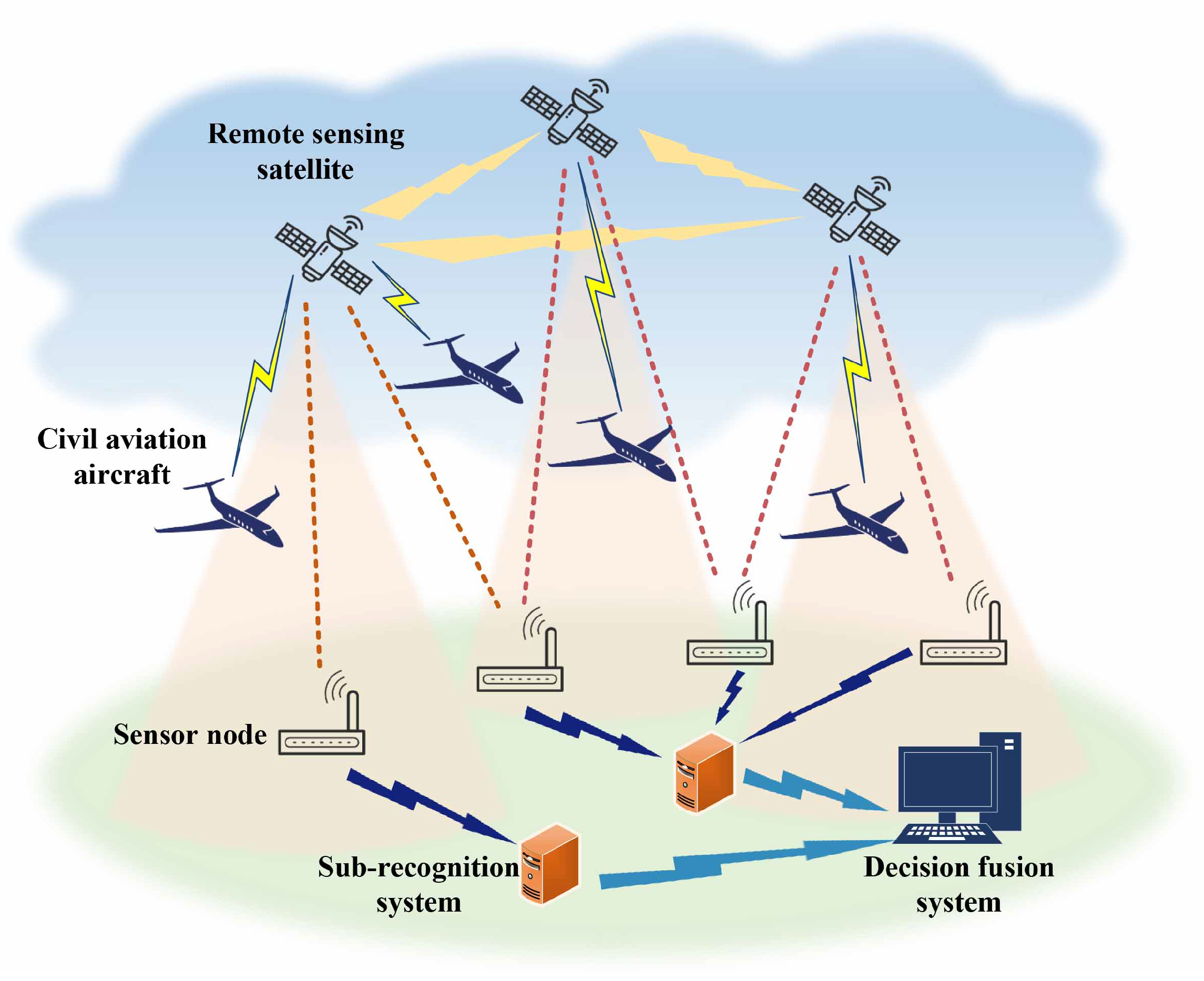
In this paper, we consider a specific emitter identification system based on ADS-B over satellite, as depicted in Figure 1. Each sensor receives ADS-B signals and employs transfer learning for SEI, forming a subrecognition system. Ultimately, the outputs from various sensors are integrated using a decision fusion system. The signal reception process in the system can be described as
where represents the ADS-B signal, denotes the transmission channel, and signifies additive Gaussian noise. The signal power is , the noise power is , T represents one complete cycle of the signal , and the signal-to-noise ratio is defined as SNR .
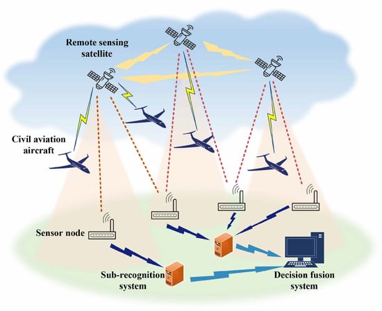
Figure 1.
Specific emitter identification system model.
We utilize the BST to extract the “fingerprint information” within the emitter signals to address the received ADS-B signals. Subsequently, a convolutional neural network is employed for feature extraction and classification, resulting in a trained model. To tackle the issue of decreased recognition accuracy in distributed sensor systems, we use a transfer learning approach and leverage decision fusion techniques to process the outputs from various sensors comprehensively.
3. Bispectral Feature Analysis
The bispectrum transform, known as the third-order spectrum, performs Fourier transforms on the third-order cyclic cumulant. This method remains unaffected by temporal interference, allowing for the preservation of fundamental information from the original signal and partial suppression of noise. As a result, the BST has found widespread application in the field of SEI. However, this method comes with a relatively high complexity and is often combined with techniques such as slicing or integration to achieve dimensionality reduction.
Nonparametric techniques are employed to estimate the bispectrum of the received signal, denoted as . The signal is partitioned into segments, each comprising samples. Hence, the third-order cyclic cumulant of the received signal can be expressed as [39]
where represents the third-order cyclic cumulant of each signal segment. The bispectral estimation of can be expressed as
where , and is a hexagonal window function. We can define the objective function for bispectral dimensionality reduction as
where represents the compressed bispectral projection space of the originally selected bispectral set , , and . In this context, S and D are bispectral weight matrices originating from different or the same emitter signals. When the emitters are distinct, , otherwise
If the emitters are identical, , otherwise
where is a positive real value.
Then we can rewrite (4) as
where , , ⊗ is the matrix multiplication. Let , where is a nonzero constant, so we can then express the Lagrangian function as
where serves as a weight coefficient. To achieve the minimization of (7), we establish . Subsequently, we can derive from the Lagrangian function
According to the above expression, we can calculate the elements inside the mapping matrix and consequently obtain the projection matrix , from which the compressed bispectrum can be calculated as
where is the original selected bispectrum.
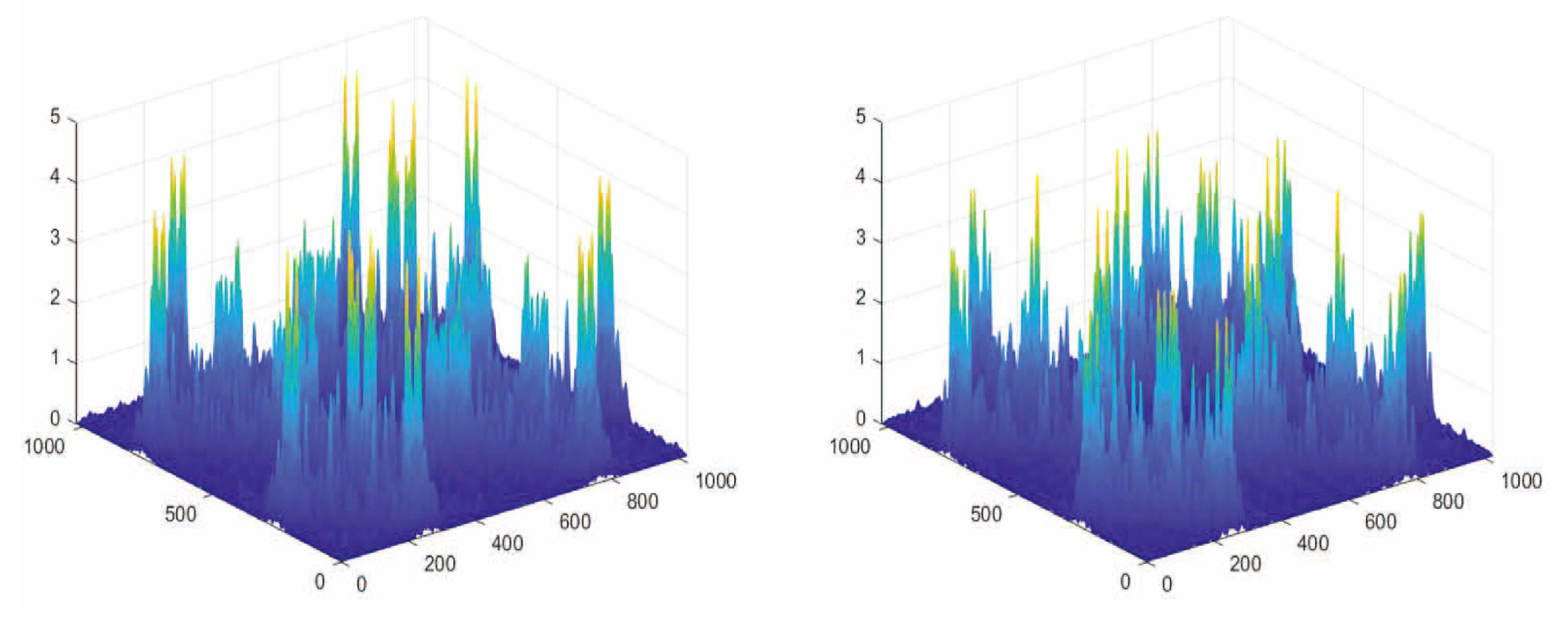
Figure 2 illustrates the bispectrum transformation diagram of an ADS-B signal. The x axis and y axis represent the two frequency components of the signal, while the z axis represents the bispectral density, indicating the strength of the interaction between these two frequency components. The lighter the color, the higher the spectral density. We can observe that the bispectral transform features of different ADS-B signals are distinct.
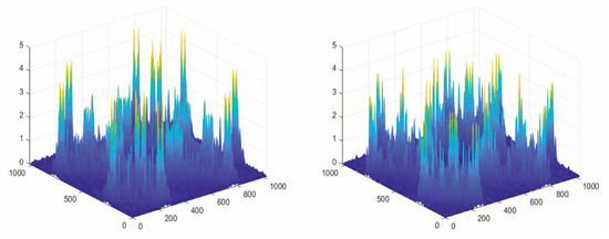
Figure 2.
Bispectrum transformation diagram of different ADS-B signals.
4. Specific Emitter Identification Based on Transfer Learning
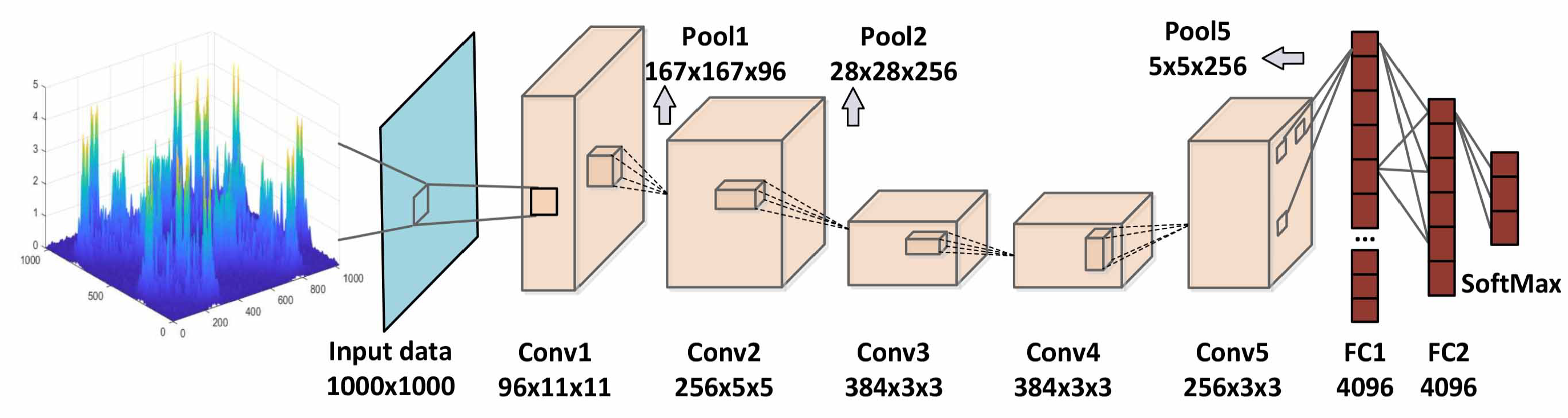
Deep learning can leverage latent features more comprehensively, thus relaxing the requirements for feature extraction. CNNs are a deep feed-forward artificial neural network that has demonstrated exceptional performance across various data recognition tasks. In this study, we employ Alex-Net as the recognition architecture, comprising 60 million parameters and 65,000 neurons. The first layer of the network includes five convolutional layers with kernel sizes and quantities of 96 × 11 × 11, 256 × 5 × 5, 384 × 3 × 3, 384 × 3 × 3, and 256 × 3 × 3, respectively. A 3 × 3 pooling layer follows each convolutional layer, facilitating data compression and reduction in computational load. Subsequently, three fully connected layers with 4096, 4096, and 1000 nodes, respectively, are incorporated. As the objective is to classify the number of individual emitters, a soft-max function is added as the output layer with M nodes (M representing the number of emitters to be identified). Additionally, to mitigate overfitting, a dropout layer is introduced following each fully connected layer. The convolutional neural network architecture employed in this paper, designed to accomplish the task of individual emitter identification, is illustrated in Figure 3. The input to the neural network consists of the bispectral density information of the signals described in Figure 2.
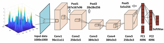
Figure 3.
Network structure for specific emitter identification.
In real-world applications, machine learning faces several challenges. For instance, there might need to be more data to support practical training in specific scenarios. For example, acquiring high-quality labeled data could be costly and difficult in medical image processing. Additionally, deep learning models assume that data follow a fixed distribution, yet real-world data distributions can change over time and space, leading to inadequate robustness of deep learning models. Hence, transfer learning emerges as a solution, leveraging pretrained models (source domain models) to enhance the desired models (target domain models) to improve training efficiency, enhance model generalization ability, and address issues like network convergence.
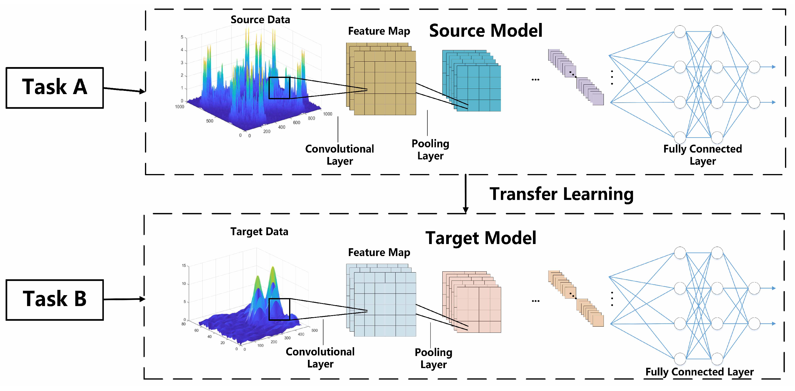
In transfer learning, several key concepts need to be clarified initially. “Domain” refers to the feature space and the marginal probability distribution (where X represents the input sample set x) of the data. Different domains possess distinct feature spaces and marginal probability distributions. “Task”, on the other hand, pertains to a specific domain and comprises the label space y and the prediction function , where is used to predict unknown data. and represent labeled data from the source domain and the target domain, respectively, while , respectively, denote the inputs and outputs of the target domain. The objective is to utilize knowledge acquired from the source domain and source task to assist in the learning of the for the target domain and target task , aiming to enhance learning performance. Figure 4 illustrates an example process of transfer learning.

Figure 4.
Example of model-based transfer learning.
4.1. Model-Based Transfer Learning
Model-based transfer learning assumes that the target domain and source domain share specific parameters or common knowledge at the model level. The source network model encapsulates expertise and experience through its network parameters and architecture. The main objective is to identify the parameter components that embody the learning outcomes. In other words, the aim is to reuse parts of the source network model and its parameters, avoiding redundant processes of data representation, experiential reasoning, and optimization when training the new task. This makes transfer learning more efficient, capturing essential information within the network.
In model-based transfer learning, two key approaches should be noted:
(1) Learning and transfer of source domain model : The source domain model must initially acquire rich knowledge from known data. The pretrained source domain model is then transferred to the target domain model, leveraging the acquired knowledge to initialize and optimize the network. With limited labeled data , a more accurate target domain model can be obtained while reducing the risk of overfitting.
(2) Determination of shared parameters: When deciding which parameters to retain and which to modify, consideration must be given to different layers of the network structure. Typically, the initial layers of the model, such as convolutional layers, function like Gabor filters, extracting shallow features like color distribution, light intensity, and contours. Conversely, the final layer of the network is often tailored to a specific task, such as animal or ethnicity classification. This suggests that the parameters of the initial layers are generalizable, while those of the final layers are task-specific. When dealing with limited target data, freezing the parameters of the general feature extraction layers while learning only the task-specific components could lead to better performance gains.
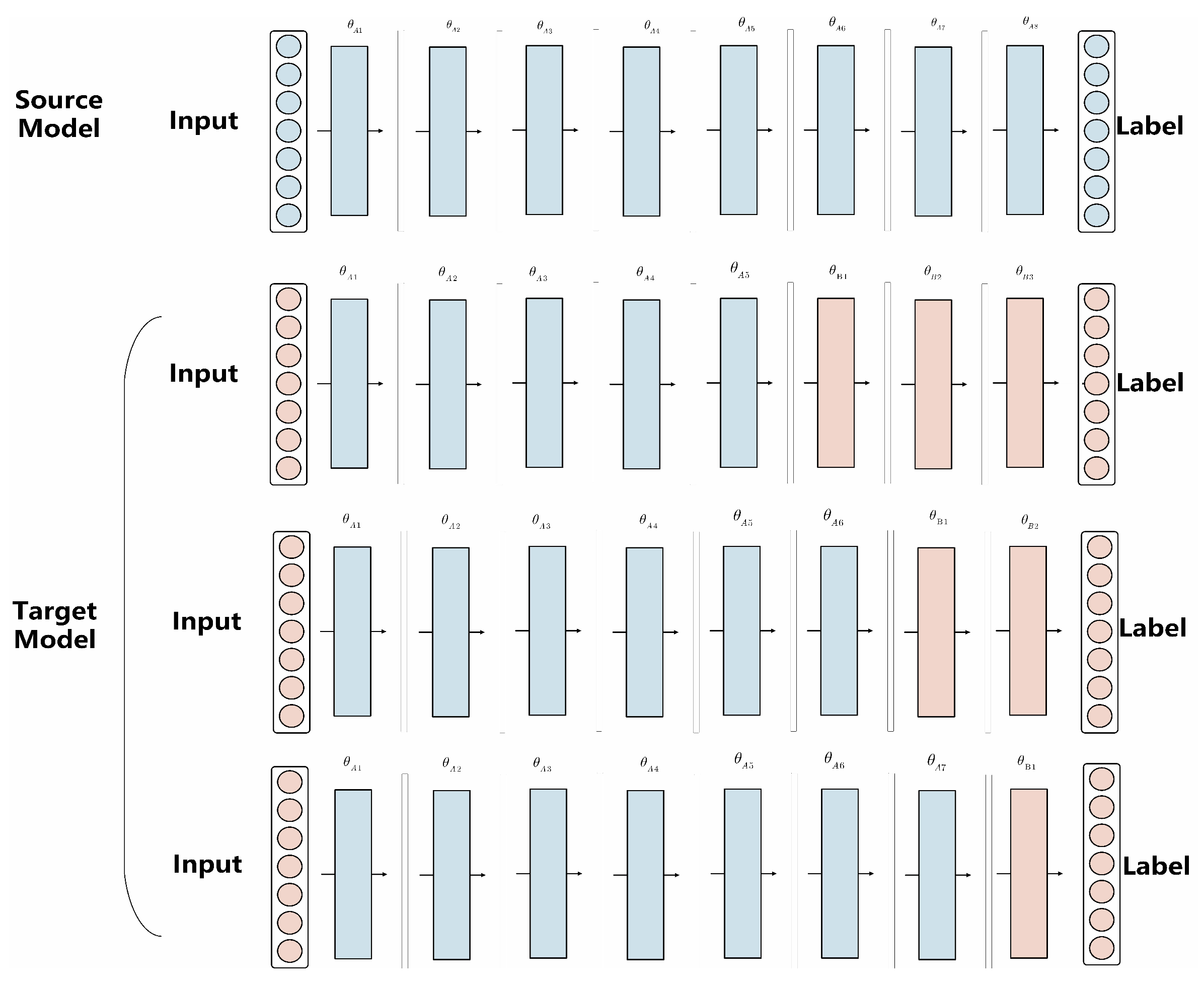
The essence of model-based transfer learning can be summarized as follows: acquire the source network model, transfer its parameters to the target network, and train the network on the new dataset. When the target dataset is small, fine-tuning all layers might lead to overfitting. Instead, freezing the parameters of the first N layers and learning only the remaining task-specific layers is recommended. Conversely, joint learning of all parameters is feasible when the target dataset is extensive. Figure 5 illustrates the concept of model-based transfer learning. Algorithm 1 outlines the training procedure for model-based transfer learning.
| Algorithm 1 Training procedure of model-based transfer learning. |
|
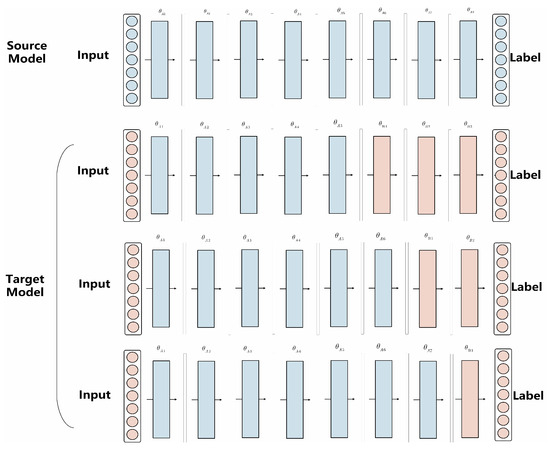
Figure 5.
Example of model-based transfer learning.
4.2. Feature-Based Transfer Learning
In the current landscape of machine learning, specific features may only hold meaning in particular domains. For instance, skin color might only be relevant for classifying different ethnicities but not in the context of fruit classification. Consequently, reusing samples from the old model to achieve transfer learning objectives becomes challenging due to inherent feature differences. To tackle this problem, this study introduces a transfer learning approach that integrates MMD with classification error. The key lies in mapping features from the original input space to an abstract space rather than directly dealing with the raw area. Specifically, we learn a pair of mapping functions, denoted as , to transform features from different domains into a shared common mapping space that contains domain-invariant features. Such mapping aids in reducing the disparity between the source and target domains, thereby achieving the objectives of transfer learning.
This paper introduces a feature-based transfer method grounded in domain adaptation theory. Firstly, we define a feature transformation T to align the joint distribution of the target and source domains, enabling them to share a common mapping in feature space. The feature transformation T can be expressed as [40]
where represents the conditional probability distribution. This paper employs principal component analysis (PCA) to perform dimensionality reduction and reconstruction of errors. In other words, we seek an orthogonal transformation matrix to maximize the variance of the embedded data, achieved by optimizing the following expression:
where represents the identity matrix, , is the input feature matrix, denotes the trace of a matrix, and the equation can be optimized as an efficient solution to the eigenvalue decomposition , with representing the top k largest eigenvalues.
The distribution discrepancy between domains needs further refinement, and in this paper, the MMD is employed to quantify the distance between domains. MMD is a nonparametric metric, which can be estimated as
where denotes the sample set of the source domain, represents the sample set of the target domain, and maps each sample to the Hilbert space using the kernel . , respectively, denote the sizes of the source and target domain sample sets. Substituting this into PCA yields
Simplify it through the kernel function
where is defined as
In addition to MMD, this paper also aims for the transfer learning paradigm to contribute to the representation of the classifier. This requires minimizing the loss function as much as possible, i.e.,
where denotes the classification loss of the model concerning the actual labels y and input data . Meanwhile, represents the distance between the source data and the target data , with being a hyperparameter that governs the level of domain confusion. It is imperative to establish . Setting too low renders the MMD regularizer ineffective on the learned representation, while setting too high imposes excessive regularization, resulting in a degenerate representation where all points are too close together. For transfer learning methods, we set the regularization hyperparameter to , which makes the objective primarily weighted towards classification but with sufficient regularization to prevent overfitting [40]. Algorithm 2 outlines the training procedure for feature-based transfer learning.
| Algorithm 2 Training procedure of feature-based transfer learning. |
|
4.3. Domain-Adaptive Transfer Learning in Hyperbolic Space
While we have indeed been able to enhance recognition accuracy through feature-based transfer learning methods, they still fall short of our expectations. We are aware that MMD narrows the gap between different domains by mapping features into an abstract space, where distinct domain spaces are transformed through mapping into a common mapping space composed of domain-invariant features. Nevertheless, we can reconsider delving again into the hierarchical relationship information of training samples, further probing their associations to enhance the expressive capabilities of the model. This endeavor contributes to rendering the source network model more comprehensive, thereby further amplifying the effects of transfer learning. In recent years, hyperbolic space has gradually found its way into deep learning and has been extensively applied. Its unique strengths, such as aiding information mining and enhancing model expressiveness, aptly align with the goal of improving transfer learning outcomes [41].
Hyperbolic geometry, also known as Lobachevskian geometry, departs from the “parallel axiom” of Euclidean geometry and instead employs the distinct “dual-sector plane axiom”, thus constituting a form of non-Euclidean geometry. This study adopts the Poincaré ball model of hyperbolic space as the spatial model, defined by , where represents the curvature of the Poincaré ball. In this model, the induced distance between any two points can be expressed as
By appending a hyperbolic network layer to the end of the original deep learning network [40] and ultimately mapping the Euclidean space onto the hyperbolic manifold , the process can be represented as
Algorithm 3 outlines the training procedure for domain-adaptive transfer learning in hyperbolic space.
| Algorithm 3 Training procedure of domain-adaptive transfer learning in hyperbolic space. |
|
5. Numerical Results and Discussion
The S-mode transponder extended squitter message protocol is one of the ADS-B link protocols. We adopt the widely used 1090ES in the extended squitter of mode S transponders as the simulation signal. The operational frequency is 1090 MHz, and the total frame length is 120 μs, with the first 8 μs being the leading pulse and the subsequent 112 μs being the data field. The leading pulse consists of four pulses with a duration of 0.5 μs, starting at times 0 μs, 1 μs, 3.5 μs, and 4.5 μs. The data field comprises 112 bits, where each bit represents a message containing information such as the position, altitude, speed, heading, and identification number of the aircraft. Pulse position modulation and binary amplitude shift keying are employed for data encoding, where a falling edge represents a data signal of “1” and a rising edge represents a data signal of “0”, indicating each message. We sample data of 5 μs length from the leading pulse of the ADS-B signal, using a frequency of 600 MHz, and set the SNR in the range of −8 dB to 8 dB.
The simulation experiments were conducted on an Intel Core i9-9920X desktop computer. The CPU of this machine runs at a speed of 3.50 GHz, with 96 GB of RAM, and is equipped with two RTX2080Ti graphics cards. We conducted our experiments using MATLAB version R2018b (MathWorks, Natick, MA, USA) and PyTorch version 1.10 (Facebook AI Research, Menlo Park, CA, USA).
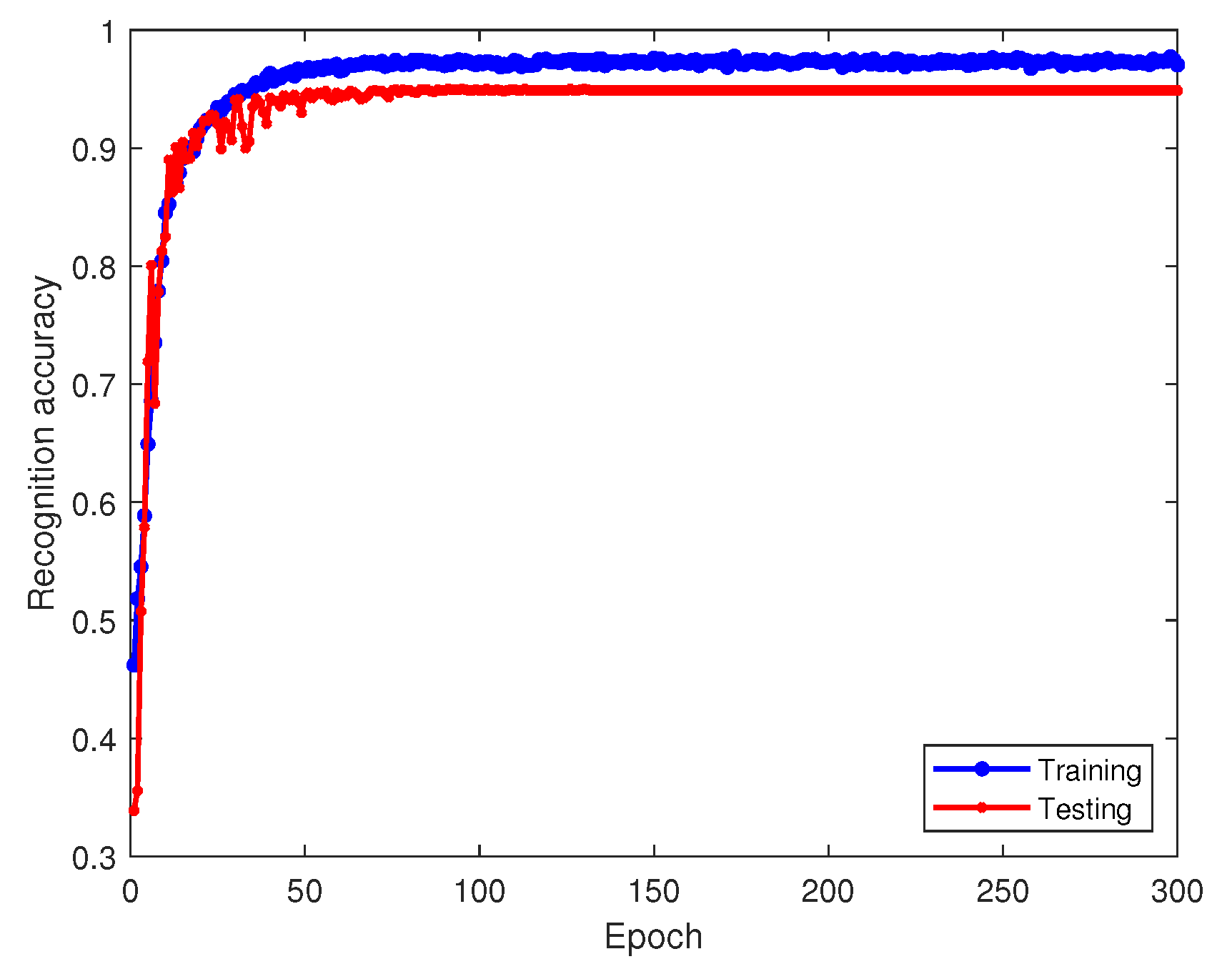
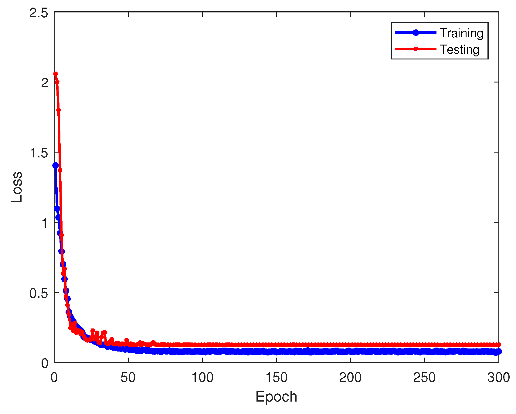
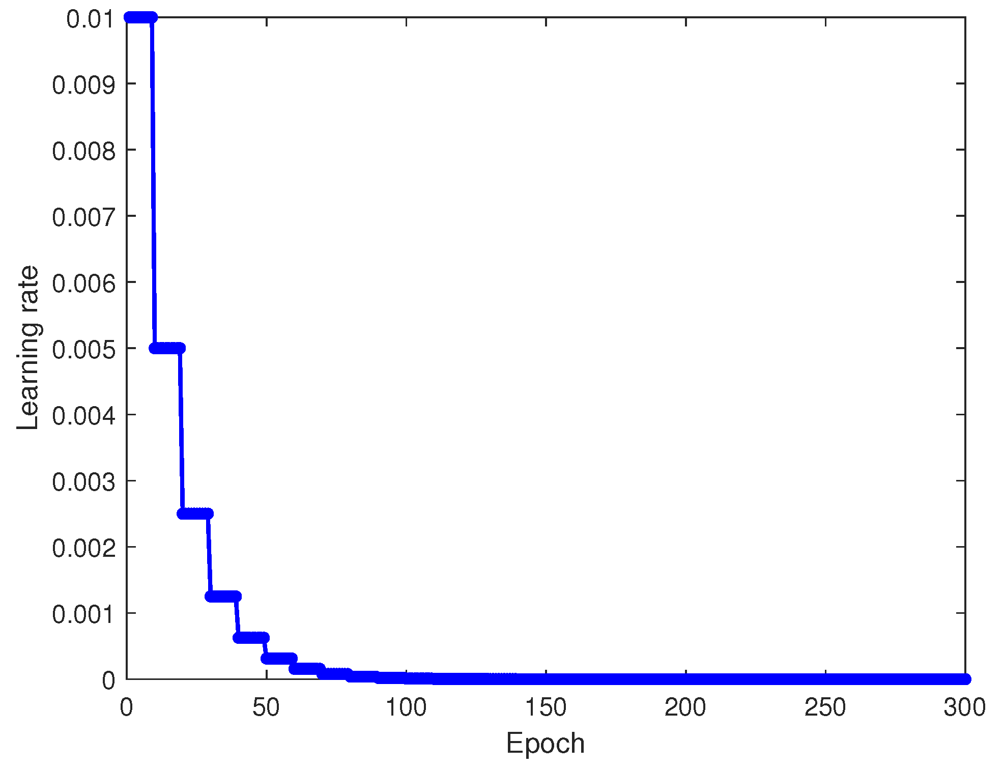
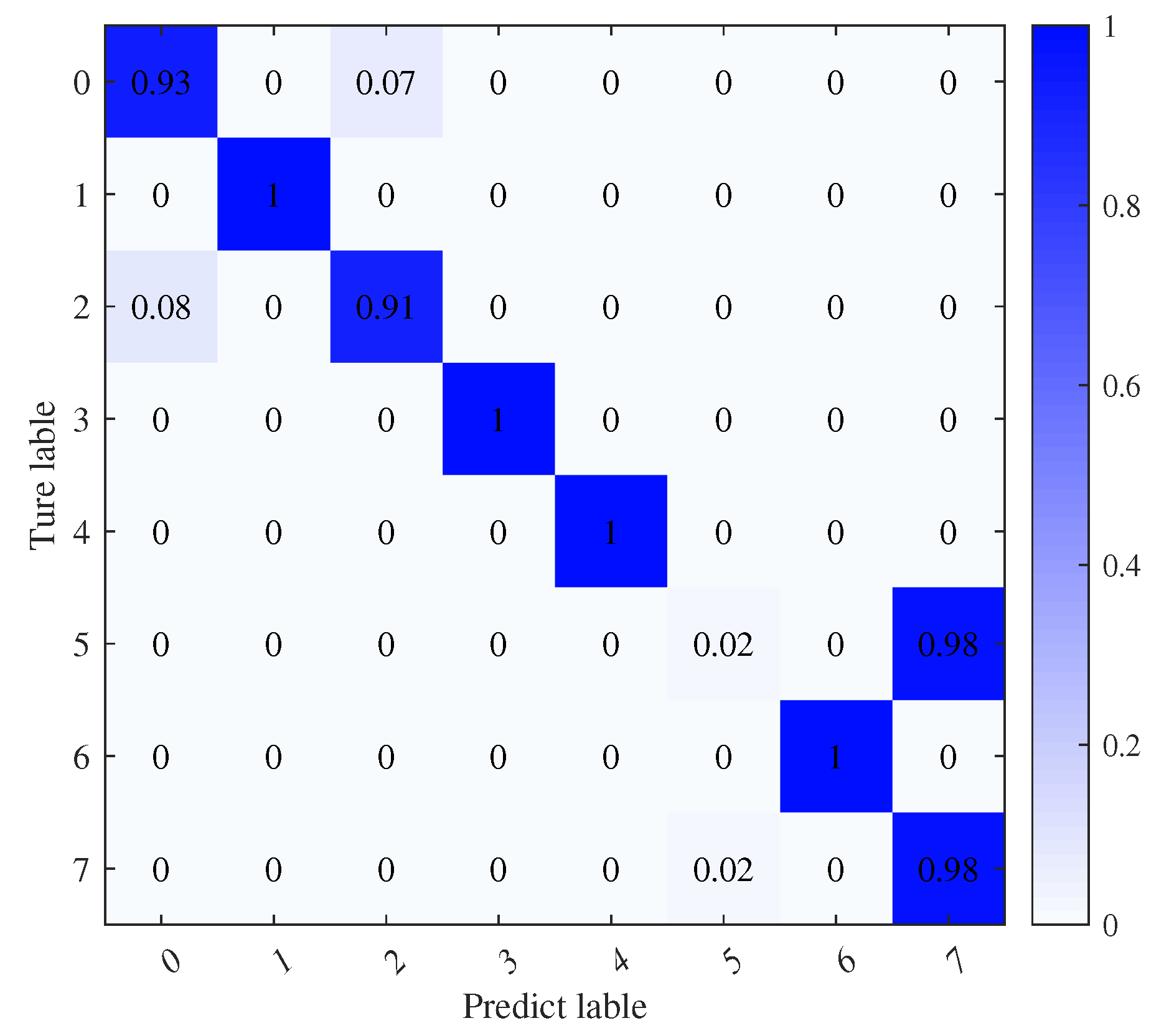
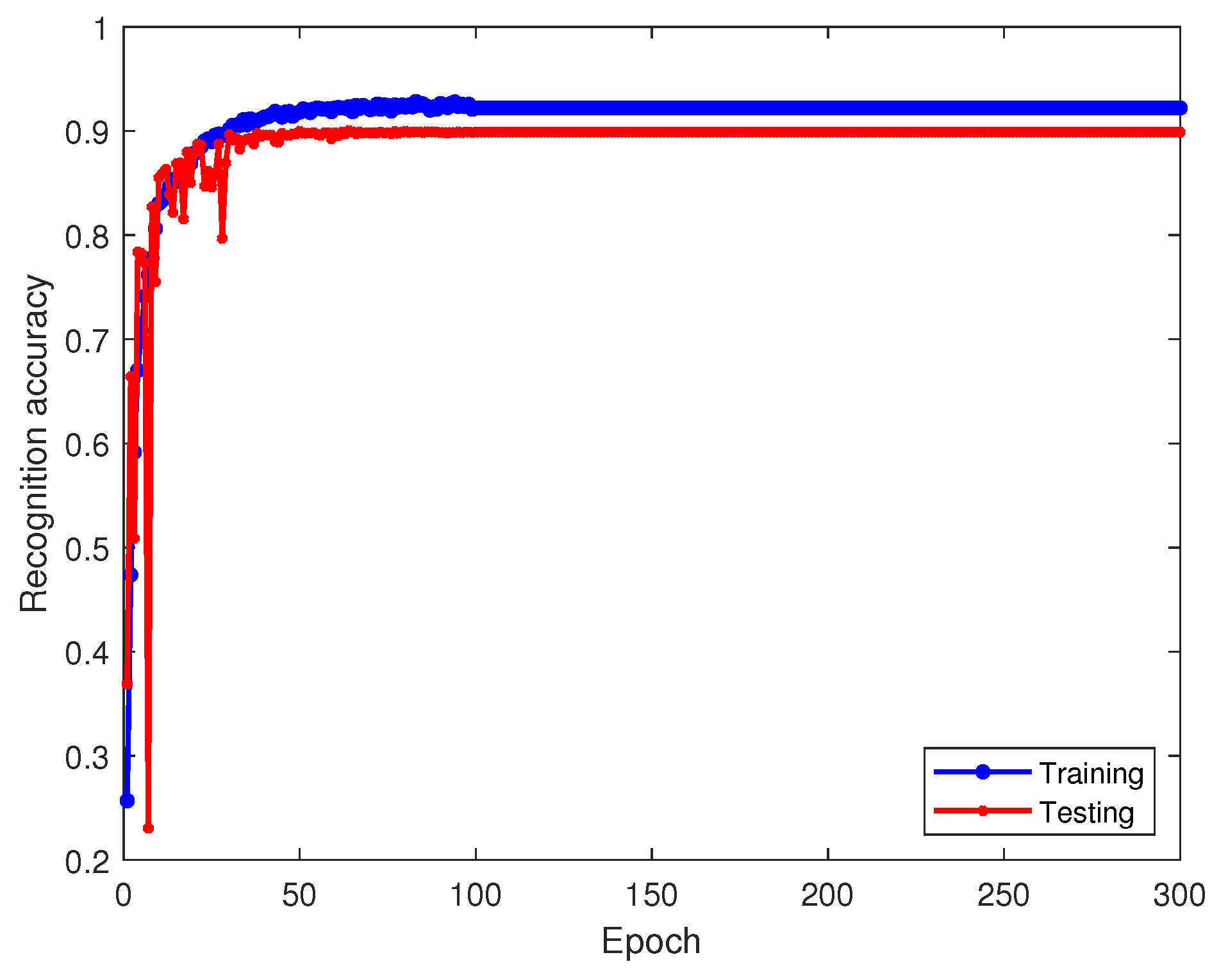
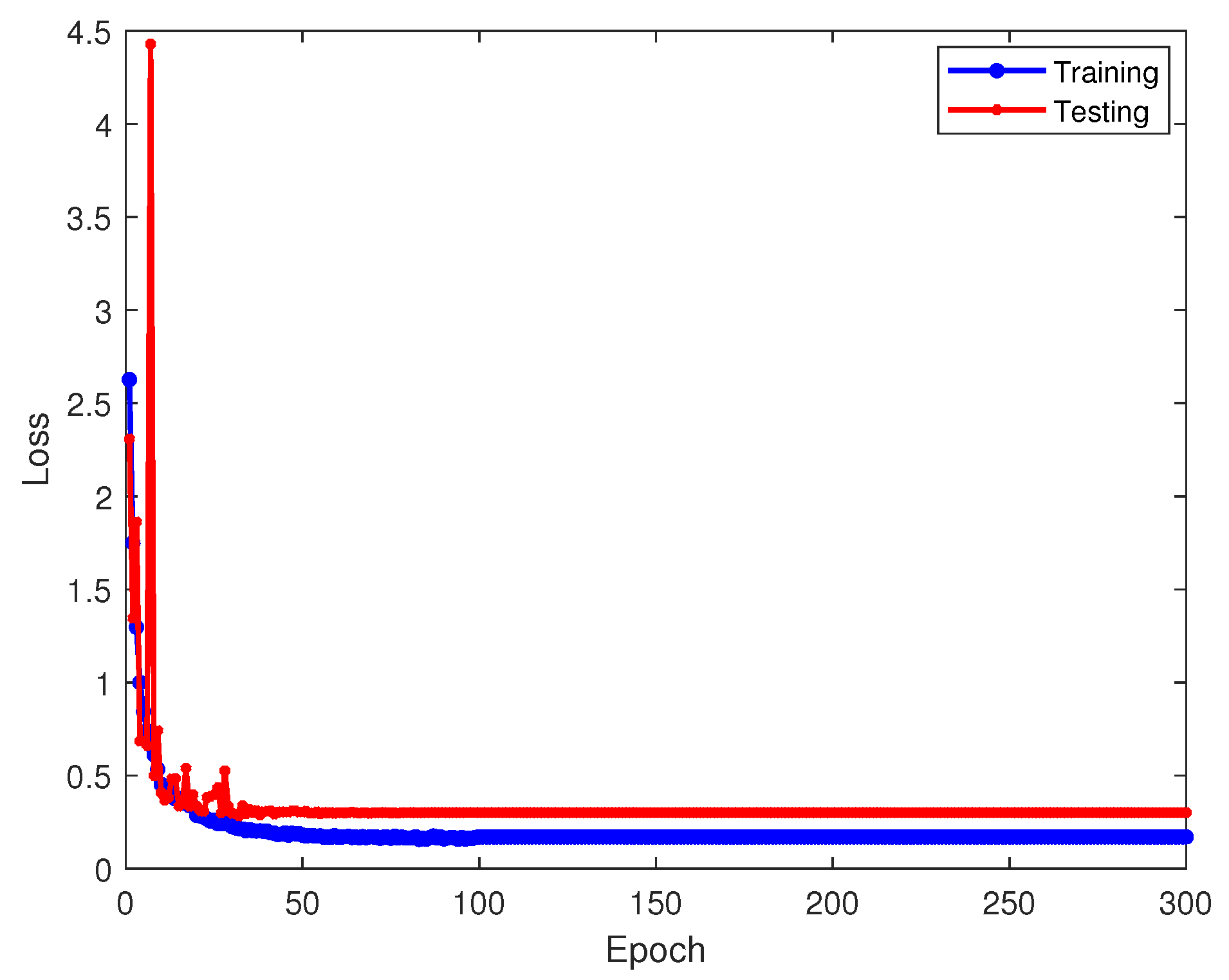
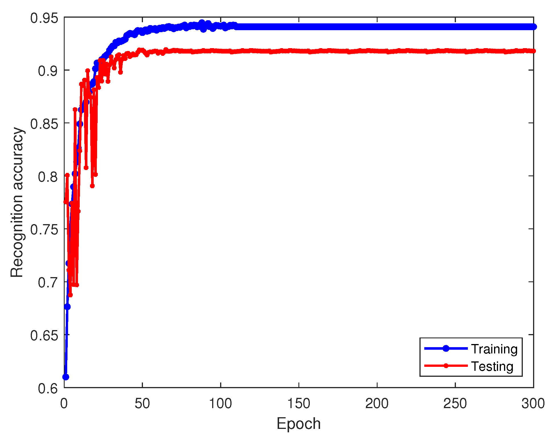
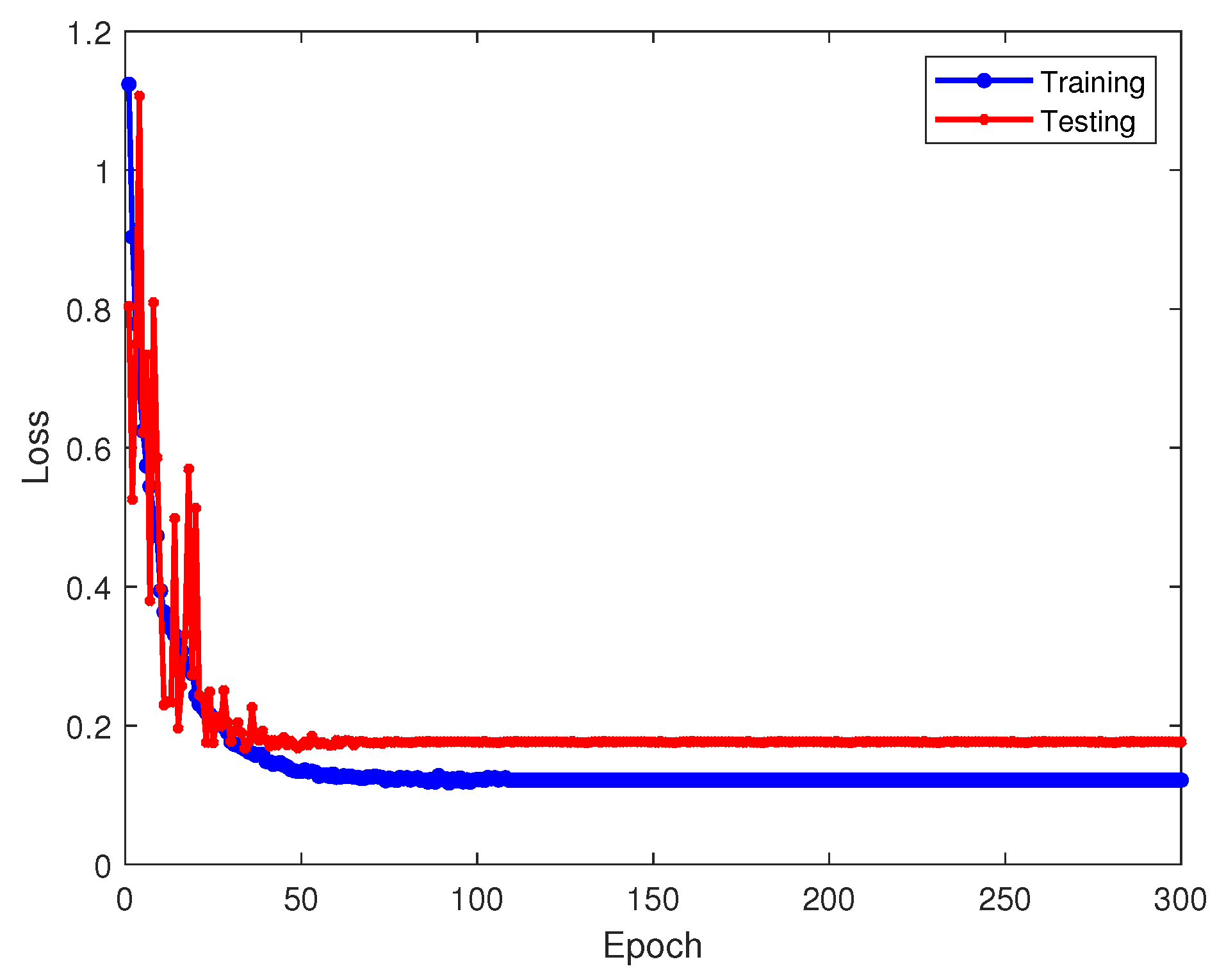
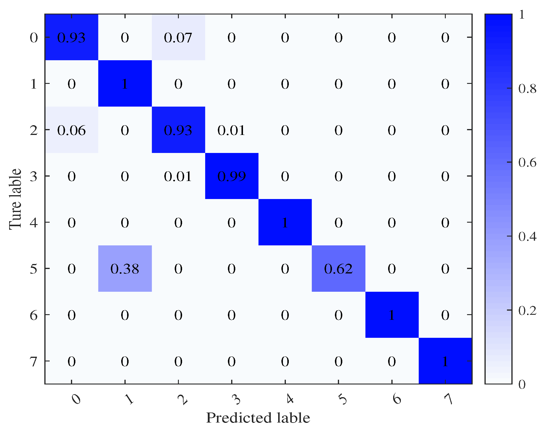
To assess the reliability of our method, we trained the source model with 1090ES simulated signals at an 8 dB signal-to-noise ratio and the transfer target model at −8 dB. Figure 6 displays the training and testing accuracy of the source model at 8 dB, while Figure 7 shows the corresponding loss values. The prediction outcomes on the test set are depicted in the output confusion matrix in Figure 8. Diagonal values represent prediction accuracy probabilities. Figure 9 depicts the progression of the learning rate across training batches. These figures indicate that at higher SNRs, signals demonstrate strong recognition performance, achieving up to a 96% average accuracy on the validation set.
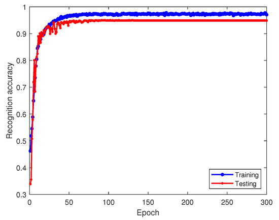
Figure 6.
Recognition accuracy of the source model on training and testing sets.
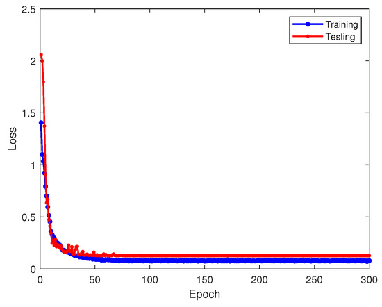
Figure 7.
Loss values of the source model on training and testing sets.
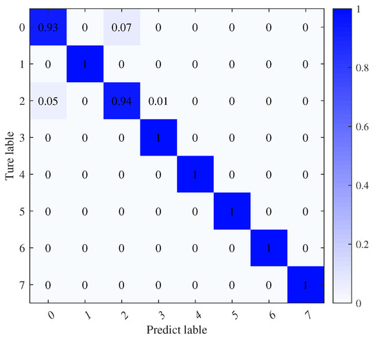
Figure 8.
Confusion matrix of the source model.

Figure 9.
Variation in the learning rate with training batches.
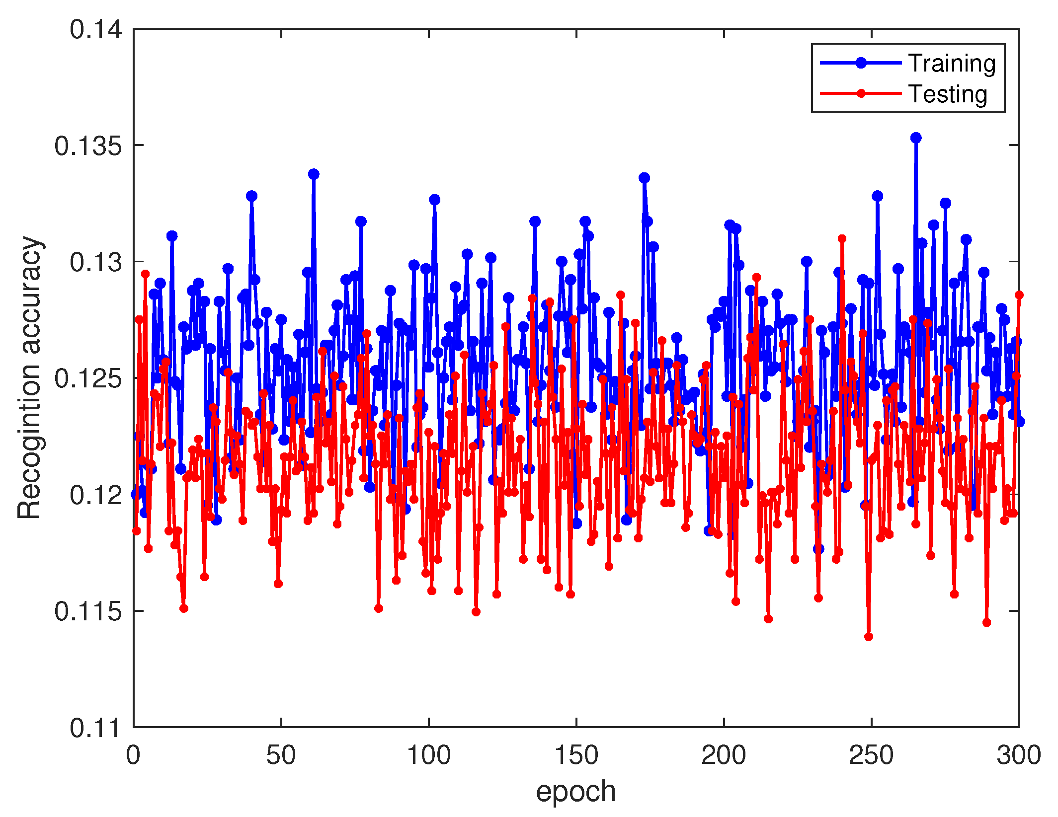
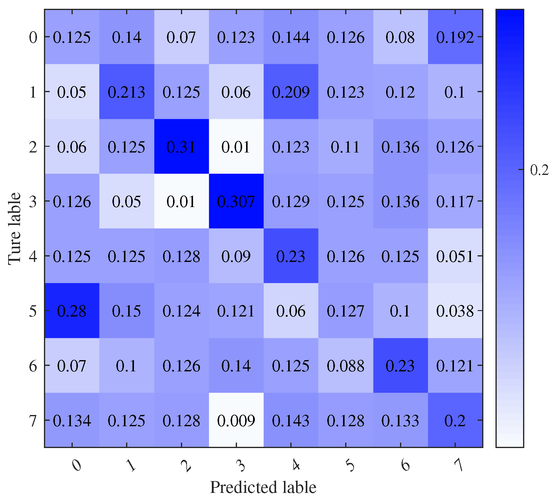
At a −8 dB SNR without transfer learning, Figure 10 and Figure 11 display the training and testing accuracies alongside the associated loss values. The test set predictions are further illustrated in the output confusion matrix in Figure 12. At a −8 dB SNR, the recognition performance significantly declines, nearly reaching random guessing levels (12.5%). As depicted in Figure 12, the neural network misclassifies all signals. In this situation, the network model becomes meaningless. However, what we need to consider is that regardless of whether it is 8 dB or −8 dB noise, the signals belong to the ADS-B signal. Their dual-spectrum transformations should exhibit the same distribution and retain many standard learning features. Therefore, this study first addresses this performance degradation issue using a model-based transfer learning approach.

Figure 10.
Recognition accuracy of directly trained target domain on training and testing sets.
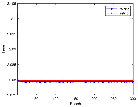
Figure 11.
Loss values of directly trained target domain on training and testing sets.
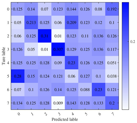
Figure 12.
Confusion matrix of directly trained target domain.
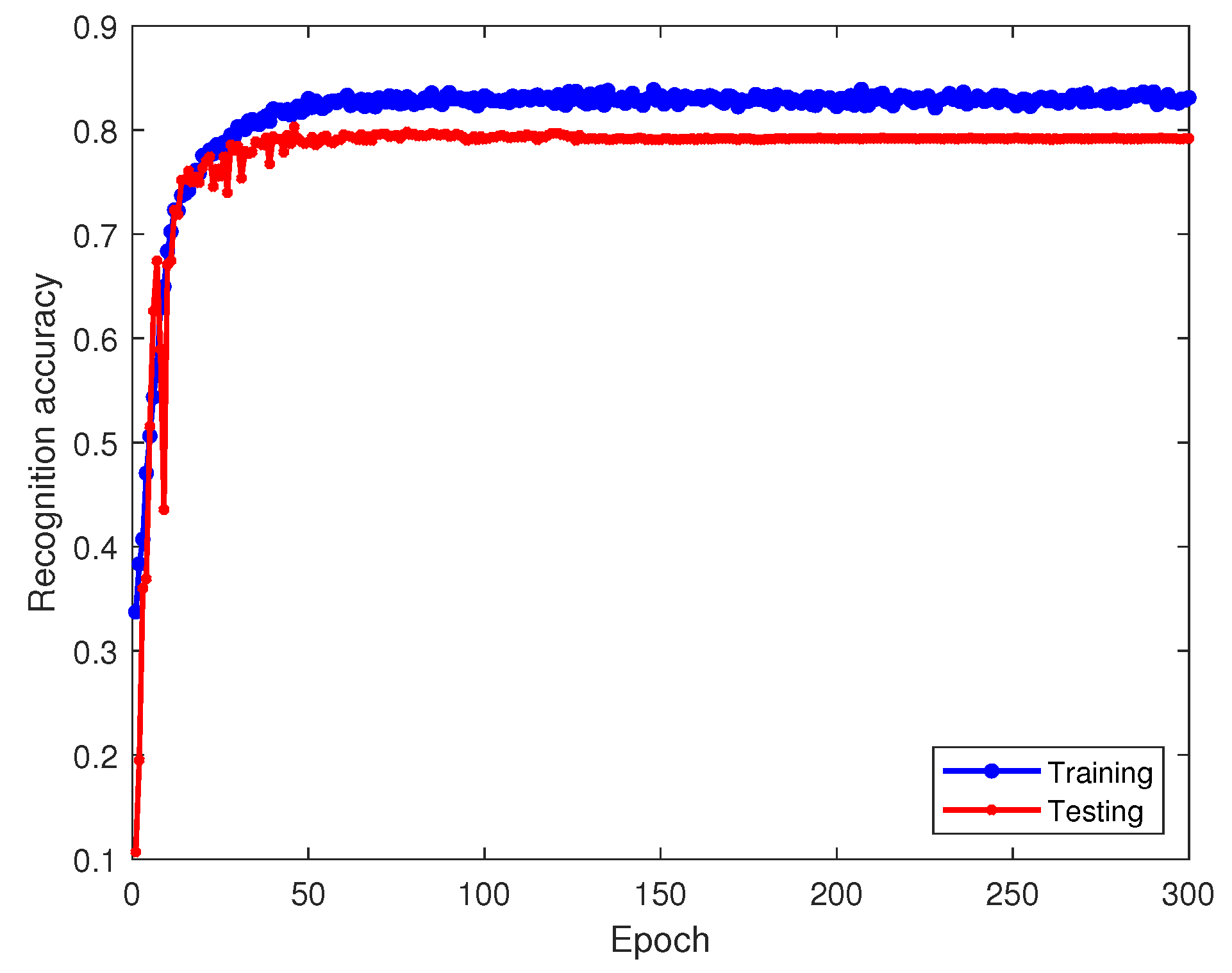
Figure 13 and Figure 14 showcase the training accuracy and loss under the transfer learning paradigm. We retain parameters from the 8 dB-trained source model, incorporate them into the −8 dB targeted model and keep the convolutional layer parameters fixed, enabling only standard updates to the fully connected layers. This strategy yields the final recognition model, with its performance depicted in the confusion matrix in Figure 15.

Figure 13.
Recognition accuracy of model-based transfer learning in the target domain on training and testing sets.
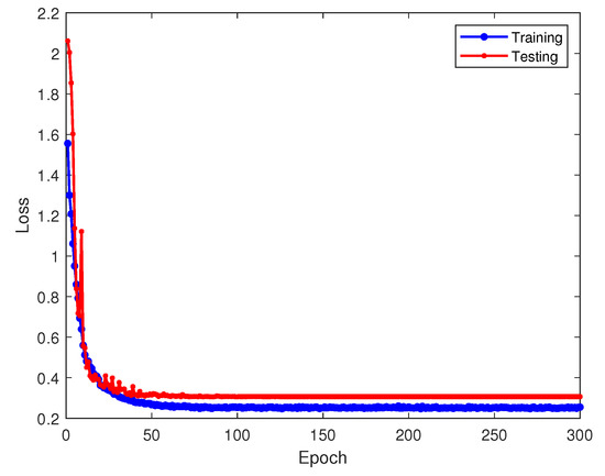
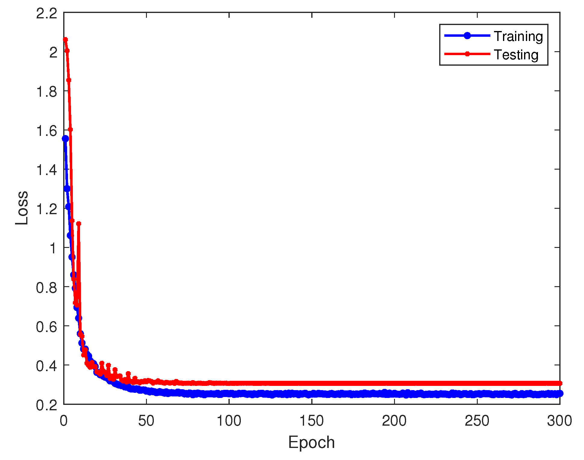
Figure 14.
Loss values of model-based transfer learning in the target domain on training and testing sets.
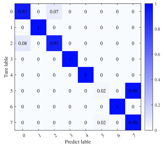
Figure 15.
Confusion matrix of model-based transfer learning in the target domain.
Figure 15 illustrates that using the model parameter sharing-based transfer learning method boosts training accuracy from about 12% to roughly 79% compared to direct training with the target dataset. This illustrates that the method of transferring the source domain model and freezing the convolutional layer parameters is advantageous for initializing and optimizing the network, effectively addressing the issue of difficult convergence. However, the convolutional neural network often misclassifies the sixth-class signal, mistaking it for the eighth-class signal.
Conventionally, in transfer learning, convolutional layers remain untrained while only the fully connected layers adapt to specific tasks. Yet, determining the optimal layer for transitioning from shared to task-specific parameters and whether to freeze initial layers remains open to further exploration. These findings suggest potential enhancements in model parameter-based transfer learning.
Figure 16 and Figure 17 depict the recognition accuracy and loss of the feature-based transfer learning method, incorporating the MMD error loss. Compared to exclusive model parameter-based approaches, recognition accuracy improves by about 10%, nearing 90%. This suggests that integrating the MMD error adaptation term further refines recognition accuracy beyond fixed parameters, aligning with transfer learning goals. The confusion matrix in Figure 18 demonstrates enhanced classification for the sixth-class signal in feature-based transfer learning, indicating progress over model parameter-based methods.
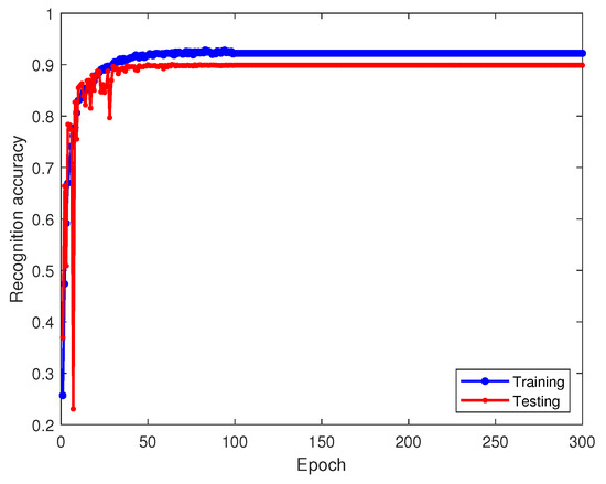
Figure 16.
Recognition accuracy of feature-based transfer learning on training and testing sets.
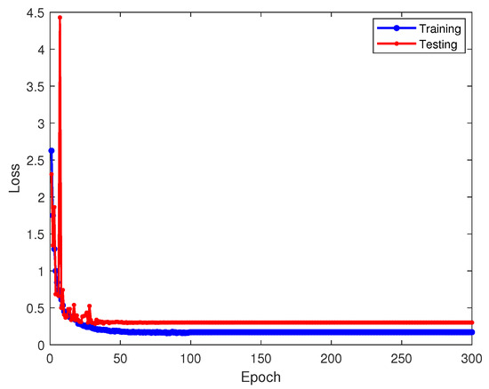
Figure 17.
Loss values of feature-based transfer learning on training and testing sets.

Figure 18.
Confusion matrix of feature-based transfer learning.
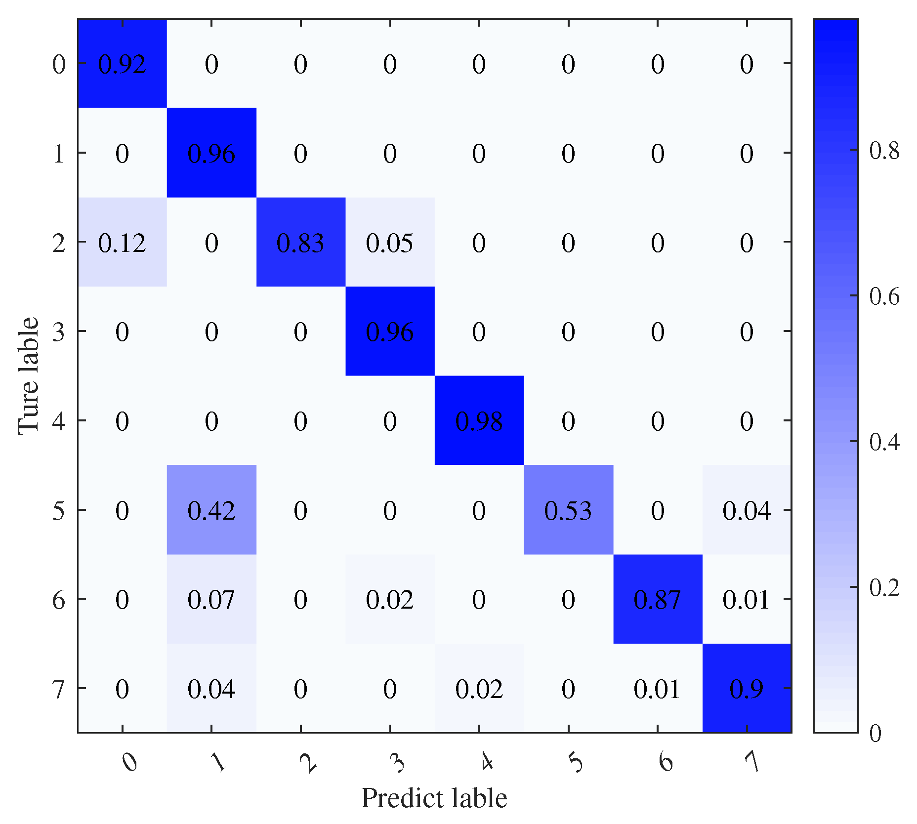
We apply domain-adaptive transfer learning within hyperbolic space to bolster recognition accuracy, as detailed in Figure 19 and Figure 20 for accuracy and loss trends and Figure 21 for the confusion matrix.
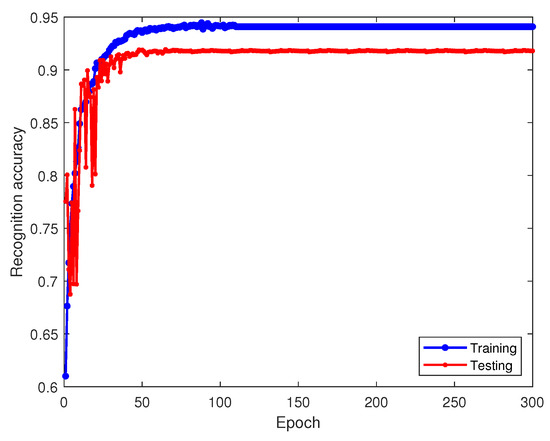
Figure 19.
Recognition accuracy of hyperbolic space-based transfer learning on training and testing sets.
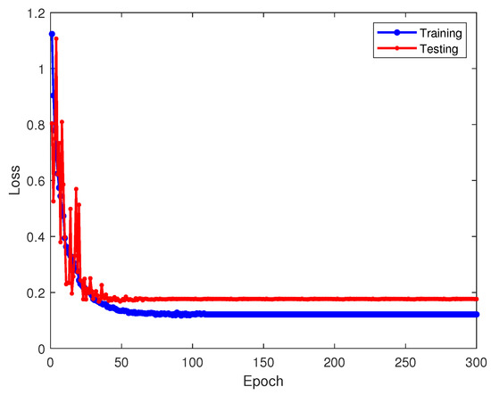
Figure 20.
Loss values of hyperbolic space-based transfer learning on training and testing sets.
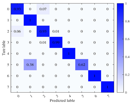
Figure 21.
Confusion matrix of hyperbolic space-based transfer learning.
Analyzing Figure 19, Figure 20 and Figure 21 reveals the advantages of leveraging hyperbolic space, facilitating enhanced model expressiveness and capturing hierarchical signal relationships. The test dataset yields a recognition accuracy of approximately 92%. This outperforms the MMD error domain adaptation approach by roughly 2% and notably elevates recognition for the sixth-class signal.
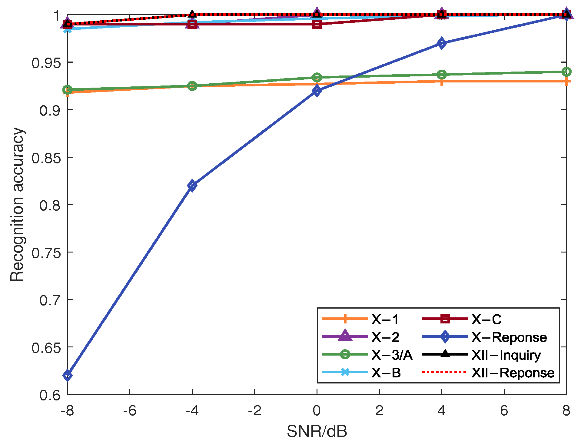
We conducted simulation experiments to validate the efficacy of our method, exploring diverse Doppler shifts, SNRs, and ADS-B signal channels. Figure 22 demonstrates consistent recognition accuracy across most signal classes at varied SNRs, highlighting the effectiveness of noise suppression in the method. It can be observed that when the SNR is greater than 0 dB, the recognition rates of various types of signals after transfer learning all exceed 90%. Furthermore, with changes in SNR, the recognition rates of most signals show no significant fluctuations, indicating the high robustness of the proposed method. Specifically, the model trained at an 8 dB SNR undergoes transfer learning to adapt to lower SNR signals.
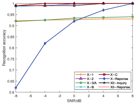
Figure 22.
Recognition accuracy of various signal classes under different SNRs.
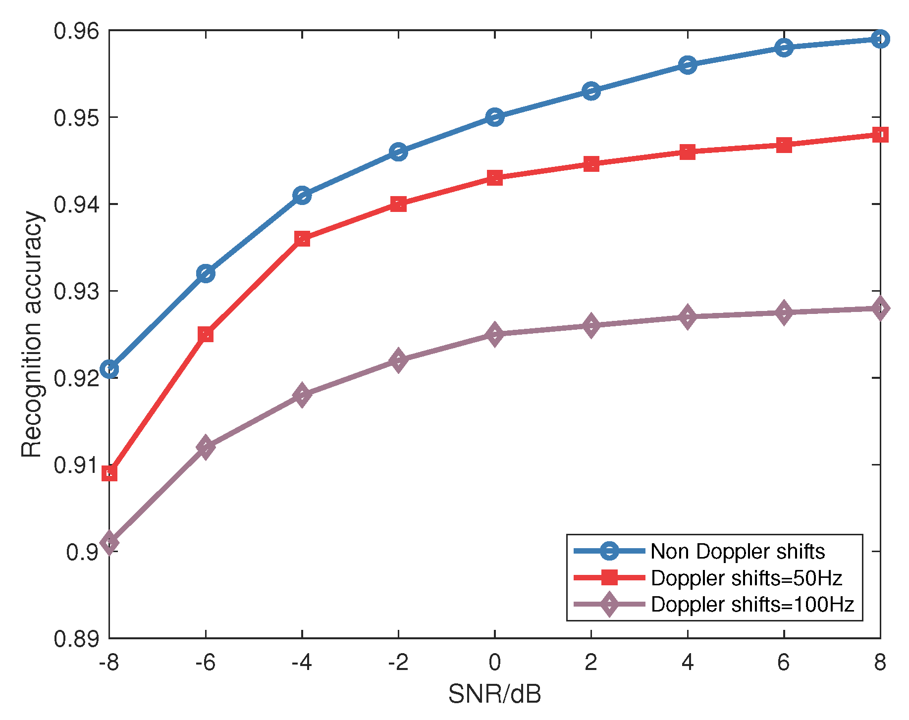
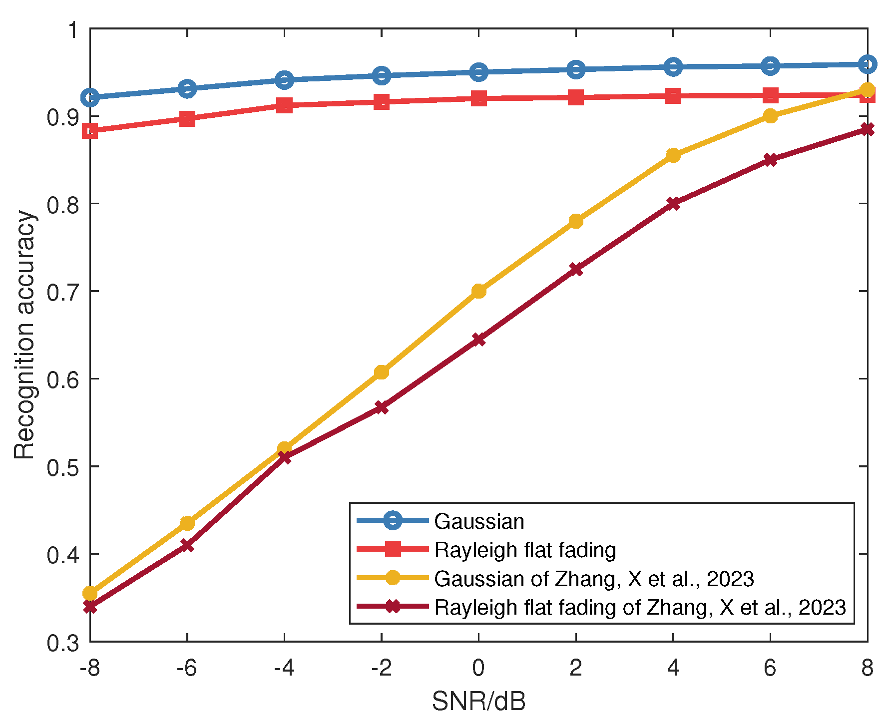
Figure 23 depicts recognition accuracy fluctuations with varying Doppler shifts. It can be observed that the phenomenon of Doppler shift affects recognition accuracy, with lower Doppler shifts corresponding to higher accuracy rates. Although Doppler shift influences accuracy, transfer learning ensures a recognition accuracy of over 90% at a Doppler shift of 100 Hz, highlighting enhanced robustness. Figure 24 examines average recognition accuracy across Rayleigh flat fading and Gaussian channels. The approach proposed by Zhang, X. et al. [27] is used for comparison. It employs a domain adversarial neural network to generate domain-invariant fingerprint features, thus achieving SEI. By comparison, the recognition accuracy of the proposed CNN network framework for identification surpasses that of the existing literature in both Gaussian and Rayleigh channels. When SNR is above −8 dB, the average recognition accuracy still exceeds 85%; while Rayleigh conditions marginally reduce recognition, the decline remains insignificant, affirming the adaptability of the method to Rayleigh fading.
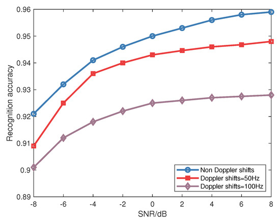
Figure 23.
Average recognition accuracy for signals with different Doppler shifts.
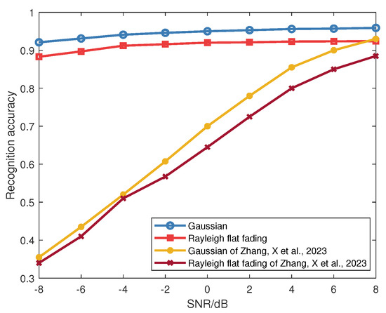
Figure 24.
Comparison of recognition accuracy for signals under Rayleigh flat fading and Gaussian channels with [27].
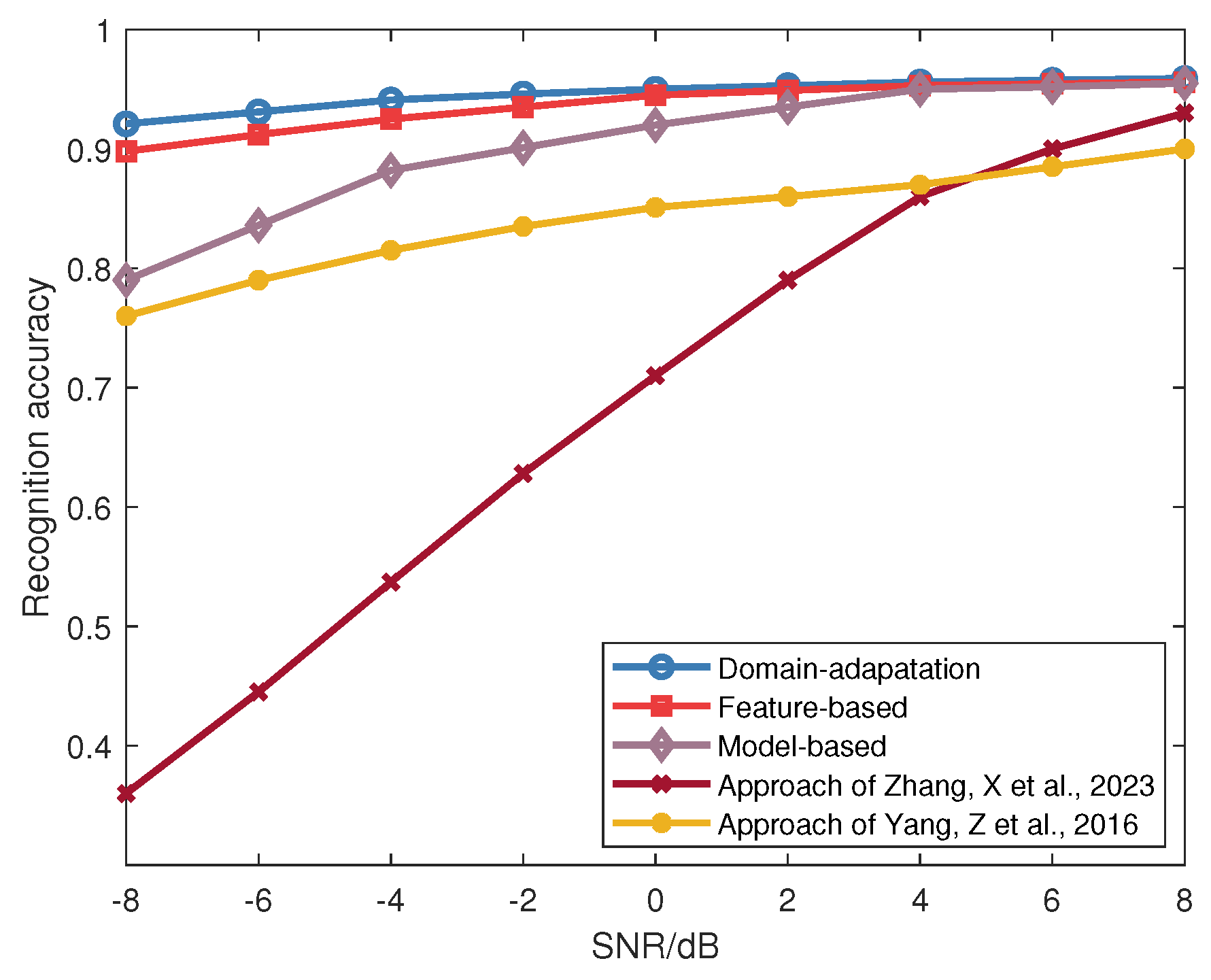
Lastly, Figure 25 contrasts the recognition accuracy of three transfer learning methods across different SNRs. The approaches proposed by Yang, Z. et al. [26] and Zhang, X. et al. [27] are for comparison. From Figure 25, it can be observed that model-based transfer learning achieves approximately 80% accuracy at an SNR of −8 dB. However, according to Figure 15, its performance on the sixth category of signals remains suboptimal. Feature-based transfer learning further refines the recognition method, elevating the recognition rate to 90% under equivalent conditions. Furthermore, the hyperbolic space domain adaptation in transfer learning enhances performance even further, yielding an ultimate recognition accuracy of about 92% at −8 dB SNR. As a result, hyperbolic space domain adaptation-based transfer learning emerges as an effective learning approach, particularly under low SNR conditions. Furthermore, the three methods proposed in this paper demonstrate higher recognition rates compared to SEI using traditional approaches, and the result indicates that the approach has robustness against SNR variation.
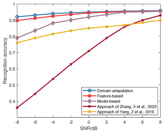
Figure 25.
Comparison of recognition accuracy for the three different transfer learning methods with [26,27].
6. Conclusions
This paper proposed an SEI framework based on transfer learning to address individual emitter recognition in an ADS-B over satellite system. Firstly, signal fingerprint information was extracted through a bispectrum transform to capture signal features accurately. Subsequently, these fingerprint details were input into a convolutional neural network to enable intelligent processing, ultimately leading to SEI recognition. A decision fusion approach was employed to tackle the problem of inconsistent identification accuracy in distributed systems. Three transfer learning methods were introduced in this paper to enhance model generalization and address the “cold start” and “slow convergence” issues in network training. Through comprehensive simulation studies, the effectiveness of this approach was confirmed. Simulation results demonstrated that transfer learning can overcome convergence challenges or slow convergence rates in various network models. Even under low SNR conditions (−8 dB), favorable training outcomes can still be achieved. Additionally, this approach exhibited a certain level of robustness in scenarios involving frequency shifts or Rayleigh fading. However, this study only considered typical Gaussian noise as the noise model, while in complex channel environments, such as in the presence of non-Gaussian noise, individual emitter fingerprints are susceptible to disturbance, increasing the difficulty of knowledge transfer. Effectively integrating transfer learning for multidimensional feature extraction in complex signal environments becomes a crucial research direction.
Author Contributions
M.L. (Mingqian Liu) conceptualized and performed the algorithm and wrote the paper; Y.C. and J.W. analyzed the experiment data; M.L. (Ming Li) helped improve the language; N.Z. is the research supervisor. The manuscript was discussed by all coauthors. All authors have read and agreed to the published version of the manuscript.
Funding
This work was supported by the National Natural Science Foundation of China under Grant 62231027 and 62071364, Natural Science Basic Research Program of Shaanxi under Grant 2024JC-JCQN-63, the Key Research and Development Program of Shaanxi under Grant 2023-YBGY-249, the Guangxi Key Research and Development Program under Grant 2022AB46002, and Innovation Capability Support Program of Shaanxi under Grant 2024RS-CXTD-01.
Institutional Review Board Statement
Not applicable.
Informed Consent Statement
Not applicable.
Data Availability Statement
The original contributions presented in the study are included in the article, further inquiries can be directed to the corresponding author.
Conflicts of Interest
Author Min Li was employed by the company Guilin Changhai Development Co., Ltd. The remaining authors declare that the research was conducted in the absence of any commercial or financial relationships that could be construed as a potential conflict of interest.
References
- Wu, Z.; Wang, F.; He, B. Specific emitter identification via contrastive learning. IEEE Commun. Lett. 2023, 27, 1160–1164. [Google Scholar] [CrossRef]
- Zhang, T.; Chen, J.; Li, F.; Zhang, K.; Lv, H.; He, S.; Xu, E. Intelligent fault diagnosis of machines with small and imbalanced data: A state-of-the-art review and possible extensions. ISA Trans. 2022, 119, 152–171. [Google Scholar] [CrossRef]
- Zhang, Y.; Peng, Y.; Sun, J.; Gui, G.; Lin, Y.; Mao, S. GPU-free specific emitter identification using signal feature embedded broad learning. IEEE Internet Things J. 2023, 10, 13028–13039. [Google Scholar] [CrossRef]
- Zha, X.; Chen, H.; Li, T.; Qiu, Z.; Feng, Y. Specific emitter identification based on complex fourier neural network. IEEE Commun. Lett. 2022, 26, 592–596. [Google Scholar] [CrossRef]
- Hao, X.; Feng, Z.; Liu, R.; Yang, S.; Jiao, L.; Luo, R. Contrastive self-supervised clustering for specific emitter identification. IEEE Internet Things J. 2023, 10, 20803–20818. [Google Scholar] [CrossRef]
- Liu, C.; Fu, X.; Wang, Y.; Guo, L.; Liu, Y.; Lin, Y.; Zhao, H.; Gui, G. Overcoming data limitations: A few-shot specific emitter identification method using self-supervised learning and adversarial augmentation. IEEE Trans. Inf. Forensics Secur. 2024, 19, 500–513. [Google Scholar] [CrossRef]
- Yang, H.; Xiong, Z.; Zhao, J.; Niyato, D.; Wu, Q.; Poor, H.V.; Tornatore, M. Intelligent Reflecting surface assisted anti-jamming communications: A fast reinforcement learning approach. IEEE Trans. Wirel. Commun. 2021, 20, 1963–1974. [Google Scholar] [CrossRef]
- Yang, H.; Xiong, Z.; Zhao, J.; Niyato, D.; Xiao, L.; Wu, Q. Deep reinforcement learning-based intelligent reflecting surface for secure wireless communications. IEEE Trans. Wirel. Commun. 2021, 20, 375–388. [Google Scholar] [CrossRef]
- Fan, S.; Zhang, H.; Zeng, Y.; Cai, W. Hybrid blockchain-based resource trading system for federated learning in edge computing. IEEE Internet Things J. 2021, 8, 2252–2264. [Google Scholar] [CrossRef]
- Lim, W.Y.B.; Xiong, Z.; Miao, C.; Niyato, D.; Yang, Q.; Leung, C.; Poor, H.V. Hierarchical incentive mechanism design for federated machine learning in mobile networks. IEEE Internet Things J. 2020, 7, 9575–9588. [Google Scholar] [CrossRef]
- Liu, M.; Zhang, Z.; Chen, Y.; Ge, J.; Zhao, N. Adversarial attack and defense on deep learning for air transportation communication jamming. IEEE Trans. Intell. Transp. Syst. 2024, 25, 973–986. [Google Scholar] [CrossRef]
- Liu, M.; Zhang, H.; Liu, Z.; Zhao, N. Attacking spectrum sensing with adversarial deep learning in cognitive radio-enabled internet of things. IEEE Trans. Reliab. 2023, 72, 431–444. [Google Scholar] [CrossRef]
- Li, Y.; Peng, W.; Zhu, X.; Wei, G.; Yu, H.; Qian, G. Based on short-time fourier transform impulse frequency response analysis in the application of the transformer winding deformation. In Proceedings of the 2016 IEEE International Conference on Mechatronics and Automation, Harbin, China, 7–10 August 2016; pp. 371–375. [Google Scholar]
- Lopez-Risueo, G.; Grajal, J.; Sanz-Osorio, A. Digital channelized receiver based on time-frequency analysis for signal interception. IEEE Trans. Aerosp. Electron. Syst. 2005, 41, 879–898. [Google Scholar] [CrossRef]
- Zhang, J.; Wang, F.; Dobre, O.A.; Zhong, Z. Specific emitter identification via Hilbert–Huang transform in single-hop and relaying scenarios. IEEE Trans. Inf. Forensics Secur. 2016, 11, 1192–1205. [Google Scholar] [CrossRef]
- Bertoncini, C.; Rudd, K.; Nousain, B.; Hinders, M. Wavelet fingerprinting of radio-frequency identification (RFID) tags. IEEE Trans. Ind. Electron. 2012, 59, 4843–4850. [Google Scholar] [CrossRef]
- Zhuo, F.; Huang, Y.L.; Chen, J. Radio frequency fingerprint extraction of radio emitter based on I/Q imbalance. Procedia Comput. Sci. 2017, 107, 472–477. [Google Scholar] [CrossRef]
- Peng, L.; Hu, A.; Zhang, J.; Jiang, Y.; Yu, J.; Yan, Y. Design of a hybrid RF fingerprint extraction and device classification scheme. IEEE Internet Things J. 2019, 6, 349–360. [Google Scholar] [CrossRef]
- Peng, L.; Zhang, J.; Liu, M.; Hu, A. Deep learning based RF fingerprint identification using differential constellation trace figure. IEEE Trans. Veh. Technol. 2020, 69, 1091–1095. [Google Scholar] [CrossRef]
- Zhou, Z.; Zhang, J.K.; Zhang, T. Specific emitter identification via feature extraction in Hilbert-Huang transform domain. Prog. Electromagn. Res. M 2019, 82, 117–127. [Google Scholar] [CrossRef]
- Xie, C.; Zhang, L.; Zhong, Z. Virtual adversarial training-based semisupervised specific emitter identification. Wirel. Commun. Mob. Comput. 2022, 2022, 6309958. [Google Scholar] [CrossRef]
- Xie, C.; Zhang, L.; Zhong, Z. Specific emitter identification with limited labelled signals based on variational autoencoder embedded in information-maximising generative adversarial network and gradient penalty. Wirel. Commun. Mob. Comput. 2022, 2022, 6185482. [Google Scholar] [CrossRef]
- Chen, P.; Guo, Y.; Li, G.; Wan, J. Discriminative adversarial networks for specific emitter identification. Electron. Lett. 2020, 56, 438–441. [Google Scholar] [CrossRef]
- Zhou, Y.; Wang, X.; Chen, Y.; Tian, Y. Specific emitter identification via bispectrum-radon transform and hybrid deep model. Math. Probl. Eng. 2020, 2020, 1–17. [Google Scholar]
- Satija, U.; Trivedi, N.; Biswal, G.; Ramkumar, B. Specific emitter identification based on variational mode decomposition and spectral features in single hop and relaying scenarios. IEEE Trans. Inf. Forensics Secur. 2019, 14, 581–591. [Google Scholar] [CrossRef]
- Yang, Z.; Qiu, W.; Sun, H.; Nallanathan, A.; Reindl, L. Emitter recognition based on the three-dimensional distribution feature and transfer learning. Sensors 2016, 16, 289. [Google Scholar] [CrossRef] [PubMed]
- Zhang, X.; Li, T.; Gong, P.; Zha, X.; Liu, R. Variable-modulation specific emitter identification with domain adaptation. IEEE Trans. Inf. Forensics Secur. 2023, 18, 380–395. [Google Scholar] [CrossRef]
- Liu, M.; Liao, G.; Zhao, N.; Song, H.; Gong, F. Data-driven deep learning for dignal classification in industrial cognitive radio networks. IEEE Trans. Ind. Inform. 2021, 17, 3412–3421. [Google Scholar] [CrossRef]
- Mei, S.; Chen, X.; Zhang, Y.; Li, J.; Plaza, A. Accelerating convolutional neural network-Bbased hyperspectral image classification by step activation quantization. IEEE Trans. Geosci. Remote Sens. 2022, 60, 1–12. [Google Scholar]
- Qian, Y.; Qi, J.; Kuai, X.; Han, G.; Sun, H.; Hong, S. Specific emitter identification based on multi-level sparse representation in automatic identification system. IEEE Trans. Inf. Forensics Secur. 2021, 16, 2872–2884. [Google Scholar] [CrossRef]
- Zhu, M.; Feng, Z.; Stanković, L.; Ding, L.; Fan, J.; Zhou, X. A probe-feature for specific emitter identification using axiom-based grad-CAM. Signal Process. 2022, 201, 108685. [Google Scholar] [CrossRef]
- Yang, N.; Zhang, B.; Ding, G.; Wei, Y.; Wei, G.; Wang, J.; Guo, D. Specific emitter identification with limited samples: A model-agnostic meta-learning approach. IEEE Commun. Lett. 2022, 26, 345–349. [Google Scholar] [CrossRef]
- Lin, Y.; Tu, Y.; Dou, Z.; Chen, L.; Mao, S. Contour stella image and deep learning for signal recognition in the physical layer. IEEE Trans. Cogn. Commun. Netw. 2021, 7, 34–46. [Google Scholar] [CrossRef]
- Yao, Z.; Fu, X.; Guo, L.; Wang, Y.; Lin, Y.; Shi, S.; Gui, G. Few-shot specific emitter identification using asymmetric masked auto-encoder. IEEE Commun. Lett. 2023, 27, 2657–2661. [Google Scholar] [CrossRef]
- Xing, Y.; Wu, B.; Wu, S.; Wang, T. Individual identification of cows based on convolutional neural network and transfer learning. Prog. Laser Optoelectron. 2021, 58, 503–511. [Google Scholar]
- Zhu, Z.; Lin, K.; Jain, A.K.; Zhou, J. Transfer learning in deep reinforcement learning: A survey. IEEE Trans. Pattern Anal. Mach. Intell. 2023, 45, 13344–13362. [Google Scholar] [CrossRef]
- Liu, J.; Yu, H.; Du, J.; Yu, W. Dynamic noise radiation source individual identification based on domain adaptation. Signal Process. 2021, 37, 1000–1007. [Google Scholar]
- Chen, H.; Yang, J.; Liu, H. Communication radiation source individual identification based on deep residual adaptation network. Syst. Eng. Electron. 2021, 43, 603–609. [Google Scholar]
- Kang, N.; He, M.; Han, J.; Wang, B. Radar emitter fingerprint recognition based on bispectrum and SURF feature. In Proceedings of the 2016 CIE International Conference on Radar (RADAR), Guangzhou, China, 10–13 October 2016; pp. 1–5. [Google Scholar]
- Long, M.; Wang, J.; Ding, G.; Sun, J.; Yu, P.S. Transfer feature learning with joint distribution adaptation. In Proceedings of the IEEE International Conference on Computer Vision, Sydney, NSW, Australia, 1–8 December 2013; pp. 2200–2207. [Google Scholar]
- Mathieu, E.; Le Lan, C.; Maddison, C.J.; Tomioka, R.; Teh, Y.W. Continuous hierarchical representations with poincaré variational auto-encoders. Proc. Adv. Neural Inf. Process. Syst. 2019, 32, 12565–12576. [Google Scholar]


Disclaimer/Publisher’s Note: The statements, opinions and data contained in all publications are solely those of the individual author(s) and contributor(s) and not of MDPI and/or the editor(s). MDPI and/or the editor(s) disclaim responsibility for any injury to people or property resulting from any ideas, methods, instructions or products referred to in the content. |
© 2024 by the authors. Licensee MDPI, Basel, Switzerland. This article is an open access article distributed under the terms and conditions of the Creative Commons Attribution (CC BY) license (https://creativecommons.org/licenses/by/4.0/).