Abstract
Over the past few years, the applications of unmanned aerial vehicles (UAVs) have greatly increased. However, the decrease in clarity in hazy environments is an important constraint on their further development. Current research on image dehazing mainly focuses on normal scenes at close range or mid-range, while ignoring long-range scenes such as aerial perspective. Furthermore, based on the atmospheric scattering model, the inclusion of depth information is essential for the procedure of image dehazing, especially when dealing with images that exhibit substantial variations in depth. However, most existing models neglect this important information. Consequently, these state-of-the-art (SOTA) methods perform inadequately in dehazing when applied to long-range images. For the purpose of dealing with the above challenges, we propose the construction of a depth-guided dehazing network designed specifically for long-range aerial scenes. Initially, we introduce the depth prediction subnetwork to accurately extract depth information from long-range aerial images, taking into account the substantial variance in haze density. Subsequently, we propose the depth-guided attention module, which integrates a depth map with dehazing features through the attention mechanism, guiding the dehazing process and enabling the effective removal of haze in long-range areas. Furthermore, considering the unique characteristics of long-range aerial scenes, we introduce the UAV-HAZE dataset, specifically designed for training and evaluating dehazing methods in such scenarios. Finally, we conduct extensive experiments to test our method against several SOTA dehazing methods and demonstrate its superiority over others.
1. Introduction
With the continuous advancement of technology, unmanned aerial vehicles (UAVs) have demonstrated outstanding performance in both military and civilian applications, attributed to their advantages such as high speed, convenience, robust maneuverability, and extensive operational capabilities [1]. However, practical applications of UAVs often encounter adverse weather conditions, especially haze [2]. Image deterioration, observed as blurring and color distortion in imaging system outputs, occurs in such hazy environments due to airborne particles absorbing and scattering atmospheric light. This degradation significantly impairs the brightness and contrast of objects, thereby impeding the normal functionality of outdoor UAV vision systems [3]. Hence, conducting further research on image dehazing methods is crucial for the further development of UAV technology.
Presently, the dominant approaches for image dehazing can be classified into two main groups [4,5,6,7]: those founded on physical models and those using deep learning. The former approach mainly focus on the mechanisms underlying the degradation of hazy images. They explore the development of physical models that conform to the degradation patterns specific to hazy images. Subsequently, parameters such as the transmission function within these models are utilized to reverse the degradation process, ultimately obtaining clear and haze-free images. As deep learning has become more popular and effective for machine vision tasks like image enhancement and segmentation, it has also begun to show promise in dehazing images. These methods leverage neural networks to learn the complex mappings between hazy images and their corresponding clear images or parameter maps, thus enabling the restoration of haze-free images.
However, it is noteworthy that current research and applications of existing image dehazing methods mainly target close-range scenes, such as indoor environments, and mid-range scenarios, such as the perspective from moving vehicles [8,9]. In these scenarios, the depth variation within a single image remains limited, resulting in a relatively consistent haze distribution across the entire image. Distinct from the aforementioned images, aerial images possess notable characteristics such as long-range views and overhead perspectives. Considering the extensive coverage in a single image, the haze density within it obviously fluctuates with changes in image depth. Existing image dehazing methods have not adequately addressed this phenomenon, leading to poor dehazing performance when adopted in long-range aerial scenes.
Considering the phenomenon mentioned above and recognizing the crucial role of depth information in predicting haze distribution in long-range aerial scenes, this paper proposes a depth-guided dehazing network (DGDN). Specifically, we first propose a depth prediction subnetwork based on multiple residual dense modules (MRDMs) to estimate the complex depth information of long-range aerial images, which further serves the subsequent dehazing process. Secondly, inspired by the attention mechanism in Transformer [10], we design a depth-guided attention module (DGAM) to couple depth maps with feature maps, leveraging depth information to guide the dehazing process, which aligns more closely with the real-world mechanism of haze formation. Finally, considering the differences between the long-range aerial perspective and other perspectives (we provide a comprehensive explanation in Section 2.3), we introduce the UAV-HAZE dataset for training and evaluating long-range aerial image dehazing methods, as shown in Section 4. The results of the experiments clearly demonstrate that the network we propose surpasses existing SOTA dehazing networks in terms of performance for both synthetic and real-world images.
To summarize, this article’s primary contributions can be described as follows:
- A depth prediction subnetwork based on multiple residual dense modules is proposed to effectively accomplish depth estimation tasks for long-range aerial images.
- A depth-guided attention module, which couples depth information with dehazing features, is proposed, which utilizes depth information to guide the dehazing process.
- The UAV-HAZE dataset is introduced, which includes approximately 35,000 synthetic hazy images captured from UAV aerial perspectives, along with their corresponding clear images and depth maps. Additionally, the dataset contains about 400 real-world hazy images. All of them are utilized for training and evaluating dehazing methods for long-range aerial images.
- Experiments are performed by utilizing both synthetic and real-world images. In addition, comparisons are carried out with several SOTA methods. Furthermore, an ablation study is performed to illustrate the benefits of the proposed DGAM.
2. Related Works
In this section, we first review the imaging mechanism of haze images and the development history of single-image dehazing methods. Then, we provide a detailed explanation of different perspectives and scenes.
2.1. Atmospheric Scattering Model
Image dehazing involves a substantial utilization of the atmospheric scattering model, which offers a traditional framework for comprehending the imaging process of hazy pictures. This model has been further developed by Nayar et al. [11,12] after being first proposed by McCartney et al. based on the Mie scattering theory [13]. The following is a detailed description of the model:
The variables in Equation (1) are defined as follows: The imaging device collects the hazy picture , the clear image , the global atmospheric light A, and the transmission map that connects these parameters. Specifically, the function is defined as:
where represents the atmospheric scattering coefficient, while denotes the distance between the target and the imaging system.
The specific imaging process is illustrated in Figure 1. The atmospheric scattering model states that there are two primary causes of hazy image degradation. First, airborne particles absorb and scatter light from the target, making the reflected light weaker. This makes the imaging results from the detection system less bright and clear ( in the first part of Equation (1)). Secondly, environmental light, like sunlight, is scattered by atmospheric particles, creating a stronger background light than the target light, which causes the imaging results to become blurry and distorted in the second part of Equation (1). Equation (2) also suggests a tight relationship between the transmission map and the depth map. This linkage emphasizes the significance of depth information in determining the transmission characteristics of hazy scenes, leading to noticeable variations in haze density in scenes with pronounced depth changes. This introduces new challenges for image dehazing methods, which is precisely the focus of long-range aerial scenes.
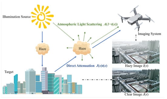
Figure 1.
The imaging mechanism of hazy weather explained by an atmospheric scattering model. The hazy weather images captured by outdoor imaging systems are coupled with two components: direct attenuation and atmospheric light scattering. The drawn materials in the image are sourced from Vecteezy (https://www.vecteezy.com/, accessed on 10 April 2024), and the photos were obtained from UAV-HAZE.
2.2. Single Image dehazing
Single image dehazing is a seriously ill-posed problem, with existing methods primarily approaching it from two perspectives: the physical model perspective and the deep learning perspective.
Physical model-based image dehazing methods typically begin with an atmospheric scattering model [14,15], estimate the global atmospheric light A and transmission map , and finally, reverse the process to generate a clear image . For example, Wang et al. [16] presented a dehazing technique for single images. Their approach utilized a physical model and employed a multiscale retinex filtering with a color restoration algorithm to enhance the brightness components of the picture. In addition to employing physical models to reverse the imaging process under haze, some methods also leverage prior knowledge for image dehazing [17,18,19,20]. By studying a huge number of outdoor hazy pictures, He et al. [17] suggested the renowned Dark Channel Prior (DCP). A simple but effective Color Attenuation Prior (CAP) was suggested by Zhu et al. [19] after they compared hazy and clear pictures in the HSV color space. Leveraging prior knowledge may enhance the effectiveness of restoring important parameters in the physical model from a statistical perspective. This, in turn, can provide guidance for the picture dehazing process and facilitate the development of a more streamlined and efficient advanced dehazing method.
There are two distinct technological ways to use deep learning-based image dehazing methods: Firstly, Equation (1) is utilized to produce the final image . Neural networks are used to predict critical parameters, such as the global atmospheric light A and the transmission map , while integrating with the atmospheric scattering model [21,22,23,24,25,26,27]. Secondly, we may immediately convert hazy images to haze-free ones by training neural networks to understand the relationship among the two types of images [28,29,30,31,32,33,34].
For the first approach, Zhang et al. [23] introduced the Densely Connected Pyramid Dehazing Network (DCPDN), which utilized a densely linked pyramid network to improve the ability to extract features. The network was designed to learn the global atmospheric light A, the transmission map , and the clear image together. This ensured that the proposed technique rigorously followed a physically based scattering model for dehazing. Li et al. [24] presented the All-In-One Network (AOD-Net), which was developed in collaboration with the atmospheric scattering model. This network integrated the global atmospheric light A and the transmission map into a unified parameter and then employed a lightweight convolutional neural network to produce the clear picture . Chen et al. [27] addressed the challenge of significant performance gaps between synthetic and real-world datasets in image dehazing. They proposed a novel network framework that leveraged pre-training on synthetic datasets and fine-tuning on real datasets using several prior knowledge. By integrating various forms of prior knowledge, they achieved domain transfer from synthetic to real domains, resulting in outstanding performance in real-world image dehazing.
For the second approach, Qin et al. [28] proposed the Feature Fusion Attention Network (FFA-Net) for image dehazing, which employed both channel attention mechanism and pixel attention mechanism to process multiscale features. Qu et al. [29] developed the Enhanced Pix2pix Dehazing Network (EPDN). Inspired by the theory of visual perceptual global precedence, they conducted dehazing operations separately on coarse and fine scales using discriminators and generators and achieved excellent dehazing results through joint training. Don et al. [31] presented a multiscale Boosted Dehazing Network (MSBDN) that utilized a local U-Net architecture. An efficient boosting decoder, grounded in the boosting and error feedback concepts, was used to gradually recover clear images, which produced remarkable dehazing achievements.
However, the aforementioned methods do not address the uneven haze density within single images due to depth variations, resulting in poor dehazing performance on long-range aerial scenes, as shown in Figure 2. In this work, we focused on utilizing the depth map to guide the dehazing process in regions with different haze densities, achieving excellent dehazing results on long-range aerial scenes.
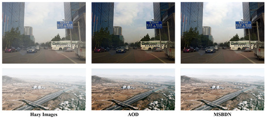
Figure 2.
The dehazing effect on different scenes. The upper row is the normal perspective image from RESIDE, and the low image is the long-range perspective image from UAV-HAZE proposed by us. It can be seen that the previous dehazing methods work well on normal perspective but cannot restore the distant areas in long-range perspective images.
2.3. Different Perspectives and Scenes
In this part, we discuss the differences between various perspectives and their distinct impacts on hazy images. Firstly, the normal perspective image is captured from ground level, resulting in images similar to what we see in our daily lives. These images are typically obstructed by objects on the ground, providing information mainly about nearby objects. Consequently, there is not much variation in depth information within a single image. Referring to Equations (1) and (2), it can be observed that the haze density across the entire image is relatively uniform. As shown in Figure 3a, existing image dehazing methods primarily rely on this perspective. For the aerial perspective commonly used in aerial dehazing methods [35,36,37], the images are captured from high altitude, resembling top-down views often seen in remote sensing imagery, as shown in Figure 3b. Due to the height of capture, the overall image tends to resemble a planar projection, with little variation in depth information caused by changes in surface objects. Degradation in these images mainly arises from the occlusion caused by aerial haze, which differs from the degradation mechanism outlined in the atmospheric scattering model. As a result, the influence of depth information on the dehazing effectiveness for such images is relatively limited. For the scenes researched in this paper, as shown in Figure 3c, this perspective, which we call long-range perspective, involves an oblique bird’s-eye view captured by UAVs from low altitude. In comparison to the normal perspective, this perspective offers a higher capturing altitude, alleviating occlusion phenomena while providing a broader field of view with richer layering within single images. Unlike the aerial perspective, this perspective offers more detailed surface object information, and the oblique angle enhances the importance of depth information within the images. In such scenes, the variations in haze density induced by changes in depth cannot be overlooked, resulting in a non-uniform haze density across the entire image. Therefore, the application of depth information is crucial for image dehazing methods in these conditions.
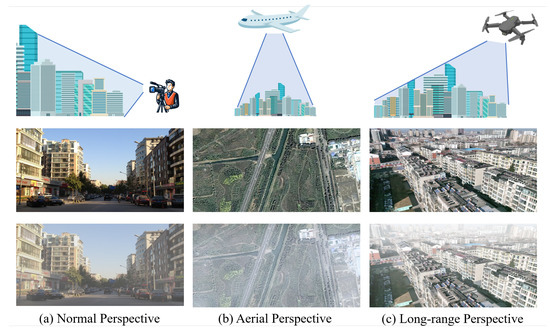
Figure 3.
Different perspectives and captured clear and hazy images (from top to bottom: diagram, clear image, hazy image): (a) Normal perspective, captured from ground level, with a limited scene span leads to a relatively average haze density; images sourced from RESIDE [38]. (b) Aerial perspective, captured from high altitude, where depth variations can be ignored, resulting in haze density being less influenced by depth; images sourced from Sate1K [39]. (c) Long-range perspective, captured from low altitude with an inclined overhead view, providing a larger span compared to (a) and more details on surface objects compared to (b); the haze density varies significantly with depth changes; images sourced from UAV-HAZE. The drawn materials in the image are sourced from Vecteezy (https://www.vecteezy.com/, accessed on 10 April 2024).
However, existing image dehazing methods have not emphasized this aspect, which is precisely the focus of this paper. As shown in Figure 2, with previous methods, the near-distance region in the image can be restored relatively clearly, while the far-distance region remains blurred. The degree of dehazing is approximately the same across the entire image, without any adaptive adjustment based on the changes in haze density. Meanwhile, it is clear that the farther regions in long-range images exhibit more serious degradation, indicating that this phenomenon is related to the depth information of the image. Therefore, this paper utilizes depth information to guide the dehazing process, making adaptive adjustments to the dehazing degree for different regions, thus achieving a more uniform and accurate dehazing performance for long-distance perspective.
3. Methodology
This section introduces the proposed depth-guided dehazing network as it shown in Figure 4. Our method comprises two branches: the depth prediction subnetwork to predict the depth map of the hazy image and the haze removal subnetwork for feature extraction. The two branches are coupled by the depth-guided attention module to achieve the fusion of depth information in the dehazing process. The details are elaborated in the following part.
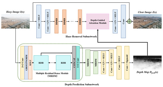
Figure 4.
The schematic illustration of the depth-guided dehazing network: (i) The haze removal subnetwork (upper branch) contains several convolution layers to change the feature map resolution (in blue), a set of DDRB to extract feature map (in orange, details in Figure 5). (ii) The depth prediction subnetwork (lower branch) contains a set of MRDM as encoder (in green) and several convolution layers as decoder (in yellow) to predict the depth map. (iii) The depth-guided attention module (in pink, details in Figure 6) uses depth information to guide the dehazing process.
3.1. Depth Prediction Subnetwork
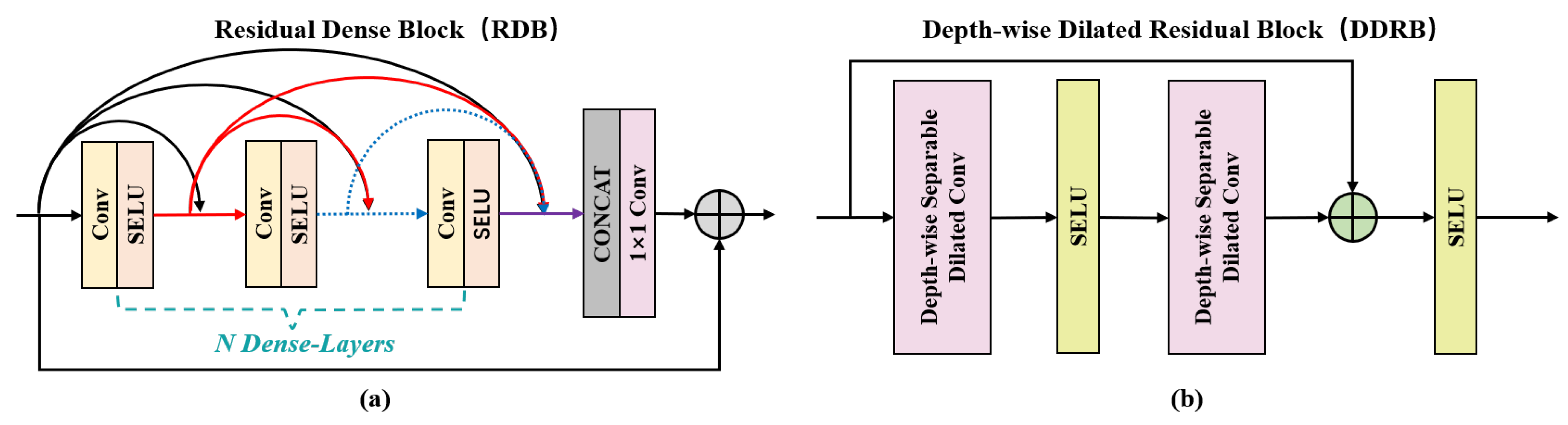
As described in Section 2.3, influenced by the shooting position of the UAV, long-range aerial images typically exhibit a top-down perspective compared to a normal perspective, with a wider shooting range. This means that long-range perspective images contain more complex, in-depth information. To enable the depth prediction subnetwork to effectively extract this depth information while keeping the process as simple as possible, inspired by the residual dense block [40], this paper proposes the Multi-Residual Dense Module (MRDM) for multiscale feature extraction and aggregation, as shown in Figure 4. The input hazy picture is reduced in resolution by first passing it through a convolutional layer, which is coupled with a groupnorm layer and the SELU activation function. The feature extraction procedure then continues through several residual dense blocks. Increasing the number of residual dense blocks could improve the network’s capacity to extract features and provide a superior output depth map. However, it also slows down the network’s runtime. Considering the trade-off between performance and efficiency, we finally adopted two residual dense blocks. The residual dense block’s form is shown in Figure 5a. In this block, the dense connection maximizes the efficient reuse of feature maps, facilitating the network to learn richer feature representations [41]. Additionally, skip connections help reduce network complexity, enhance model generalization, and accelerate model convergence [42]. Furthermore, we extended the residual dense block to a multiscale structure by constructing the residual dense blocks at different scales. This enables the network to learn richer and more diverse features, thereby enhancing its ability to represent image details. Subsequently, the multiscale feature maps go through a series of convolution and normalization layers, ultimately generating the depth map through the sigmoid function.

Figure 5.
The structure of (a) the residual dense block (RDB) and (b) the Depth-wise Dilated Residual Block (DDRB).
3.2. Haze Removal Subnetwork
The architecture of the proposed haze removal subnetwork is displayed in Figure 4. The input hazy image is first downsampled, utilizing several convolutional layers, and then passes through 11 Depth-wise Dilated Residual Blocks (DDRBs), with dilation rates set to [1, 1, 2, 2, 4, 8, 4, 2, 2, 1, 1], which can solve the gridding problem caused by single dilated convolutions [43]. The detail of the DDRB is shown in Figure 5b. By expanding the receptive field without changing the size of the feature map, this module can gather more diverse and rich feature information. Each DDRB contains two dilated convolution layers and two SELU activation functions, with the input and output feature maps connected via skip connections. The dilated convolution layers are implemented using a depth-wise separable approach, resulting in a reduction in the number of parameters in the network. This contributes to improved computational efficiency and network performance [44]. The SELU activation function possesses the self-normalizing property, ensuring that the mean and variance of the network’s output tend to stabilize [45]. This property can efficiently address the issues of gradient vanishing and gradient exploding, hence improving the training efficacy of the model. Subsequently, the feature maps undergo processing in a depth-guided attention module (DGAM) to integrate depth information. Afterward, the feature maps require resizing using convolutional layers to match the size of the input image , resulting in the residual map. Ultimately, we combine the residual map with the haze image to get the dehazed image . In the following section, the framework of the DGAM is shown.
3.3. Depth-Guided Attention Module
As mentioned in Equations (1) and (2), the haze density is closely related to depth, with this correlation being more obvious in a long-range perspective. Inspired by the self-attention proposed in Transformer [10], we introduce the depth-guided attention module to guide the dehazing process using depth information, which obtains excellent performance for long-range perspective image dehazing, the detail of this module is shown in Figure 6.
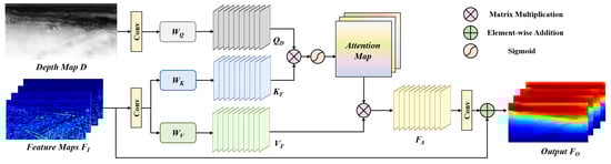
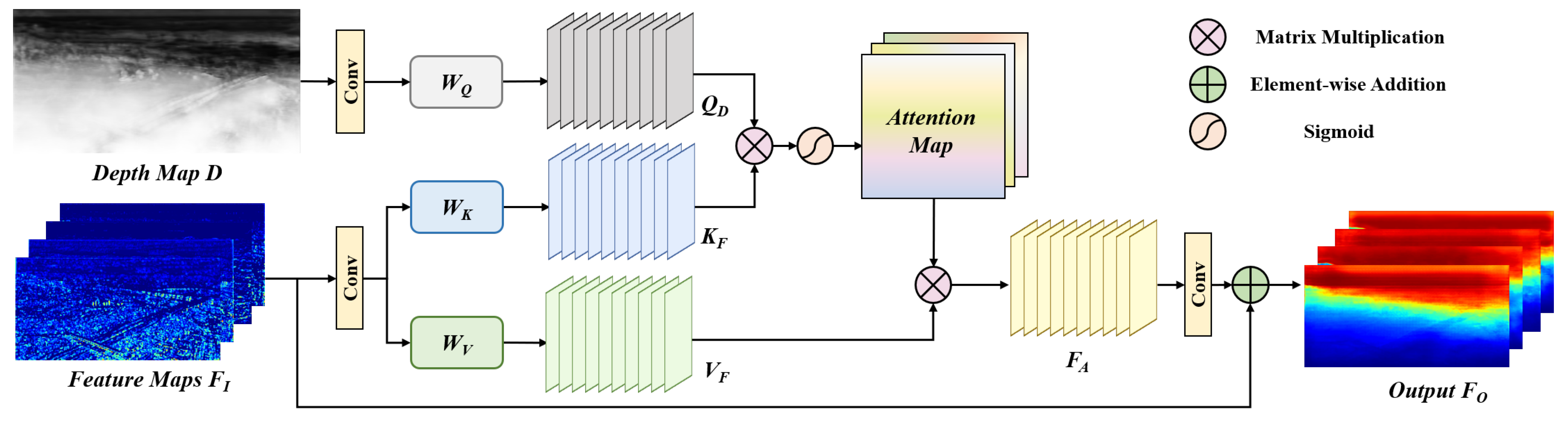
Figure 6.
The schematic illustration of the depth-guided attention module (DGAM).
Initially, the depth map obtained from the depth prediction subnetwork and the feature maps obtained from the haze removal subnetwork are the inputs of the DGAM. Then, we apply a sequence of convolutional layers to reduce the size of the feature maps to one-fourth of their original size, thereby minimizing the amount of computational memory. Following that, the feature maps are derived from the feature matrices , and , as shown in Equation (3):
where and represent the downsampled results of the depth map and feature maps . We omit in Figure 6 and the rest of this article for simplicity in writing and reading.
Next, we execute a matrix multiplication on and and then apply the Softmax layer to generate the attention maps . These maps indicate the correlation between the depth map and the feature maps, as shown in Equation (4):
where ⊗ represents the matrix multiplication, and is the transposition of .
After obtaining the attention maps , we obtain the new attention feature maps by a matrix multiplication between the feature maps and . After resizing to the same size of through the convolutional layer, we add both of them together to obtain the final output feature maps of the DGAM, as shown in Equation (5):
where ⊕ represents the element-wise addition.
In this part, we propose the depth-guided attention module inspired by self-attention. The DGAM can extract the correlation between depth map D and the feature maps of hazy images to generate an attention map and then obtain the depth-correlated attention feature maps to guide the dehazing process. This module performs well when dealing with long-range scenes with depth changes. For more details, please refer to Section 6.2.
3.4. Loss Function
The MSE loss is highly sensitive to outliers, often sacrificing the predictive performance of other normal data, leading to a decrease in the whole model performance. In addition, this loss function places more importance on global effects than on specific structures and texture information, resulting in the loss of fine details and the creation of halos or artifacts in dehazed images [46]. In order to address these issues, this article employs a joint loss function for the purpose of training.
The first step is to substitute the MSE loss with the Charbonnier loss function [47]. This function has a higher tolerance to outliers and a smoother curve, which make it more suitable for dealing with structural information for image processing. The formation of the Charbonnier loss function is:
where X represents the predicted result of the network, Y represents the ground truth, and is a constant used to prevent gradient vanishing; here, we set it to .
Then, we considered the edge information of the image from two aspects: (1) Laplacian edge detection can effectively capture high-frequency texture information; (2) the shallow layers of a CNN structure are capable of capturing low-level information such as edges and contours [48]. Therefore, we propose the edge feature loss composed of the above two parts, as shown in Equation (9):
where X, Y, and have the same meaning as described above and are not be further clarified. represents the kernel function in the Laplacian edge detection, serving as the first part of the edge extractor, while and represent the network layers before RELU1-1 and RELU2-1 in VGG-16 [49], serving as the second part of the edge extractor.
In conclusion, this paper presents the following loss function for the single image processing task:
where is the weight coefficient, and we set it to 0.8 in this work.
Given that this work involved two optimization tasks, depth prediction and image dehazing, we defined the final loss function as follows:
where is the output of the depth prediction subnetwork, while D is the ground truth of the depth map. represents the output dehazed image, and J represents the original clear image as ground truth.
4. Dataset
As mentioned in Section 2.3, in long-range scenes, the distribution of the haze density varies significantly with depth. However, existing image dehazing datasets fail to adequately capture that characteristic [38,50,51,52]. Therefore, we propose the UAV-HAZE dataset for training and evaluation for long-range scenes.
4.1. Data Collection
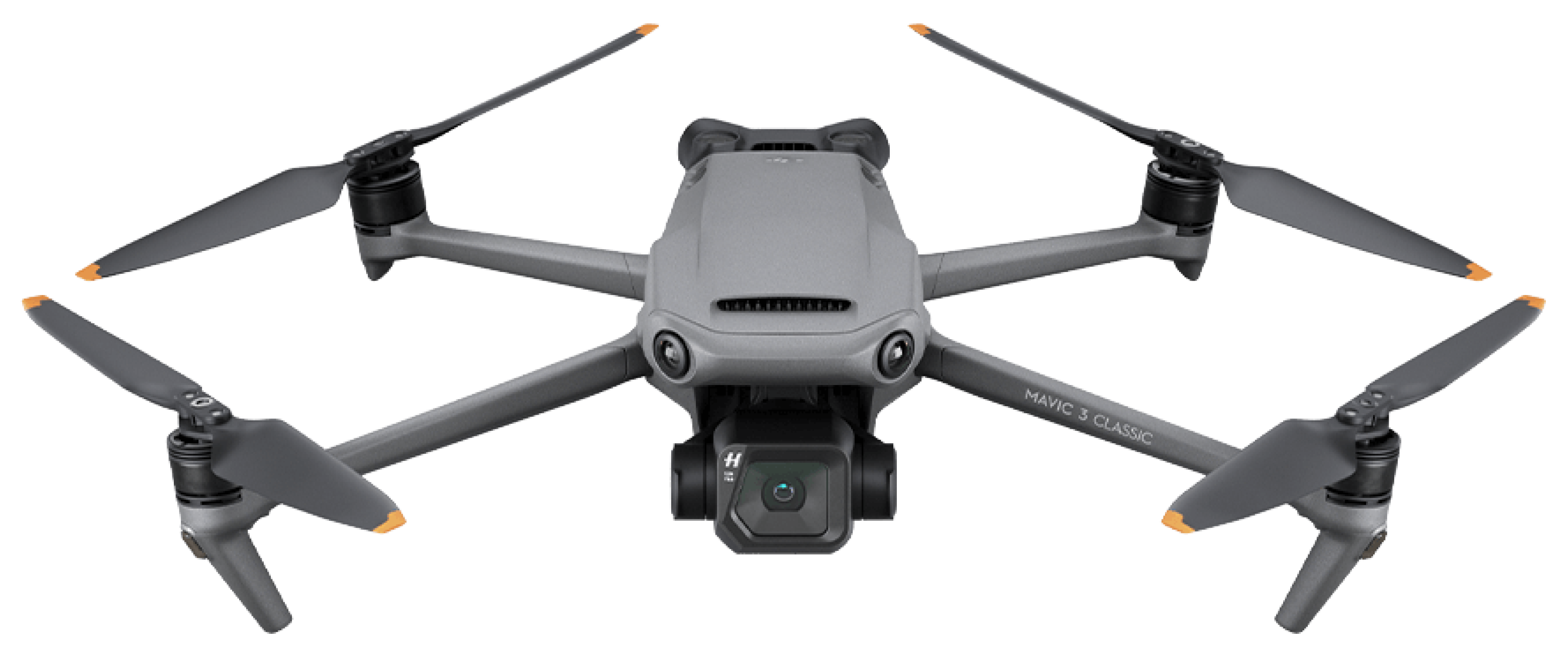
Firstly, we used the DJI Mavic 3 Classic (manufactured by DJI, shenzhen, China) to collect raw videos in different scenarios. The image of the UAV is shown in Figure 7, and its key parameters are listed in Table 1. The video files we acquired included videos in good lighting environments for generating synthetic hazy images, as well as videos in real haze conditions for generating real-world hazy images, which included multiple kinds of scenarios such as urban environments and wilderness environments, as shown in Figure 8. The video capture frame rate was 60 FPS, the resolution was 3840 × 2160 pixels, and the file format was “mp4”. We obtained 60 sequences for synthetic images and 20 sequences for real-world images. Afterwards, we extracted the original picture every 3 s from the video sequences in order to guarantee scene diversity and prevent excessive repetition, which would have decreased the quality of the dataset. In order to prepare for future network training and evaluation, we further reset the resolution to 1024 × 512. This was all the setup work required for generating the dataset.
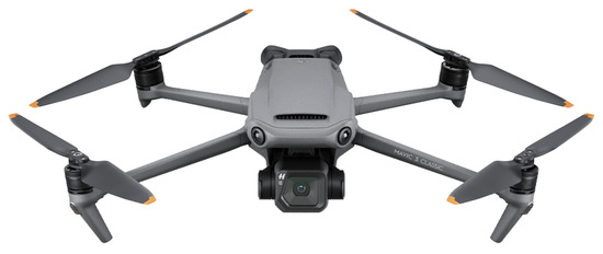
Figure 7.
The DJI Mavic 3 Classic UAV. Image from https://www.dji.com/cn/mavic-3-classic (accessed on 10 April 2024).

Table 1.
The main parameters of DJI Mavic 3 Classic.
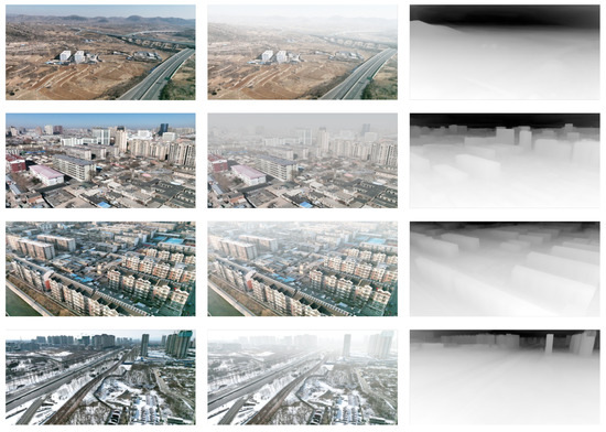
Figure 8.
Samples of the UAV-HAZE dataset. From top to bottom: different scenarios, including urban and wilderness scenes. From left to right: clear image, hazy image, and its depth map.
4.2. Dataset Introduction
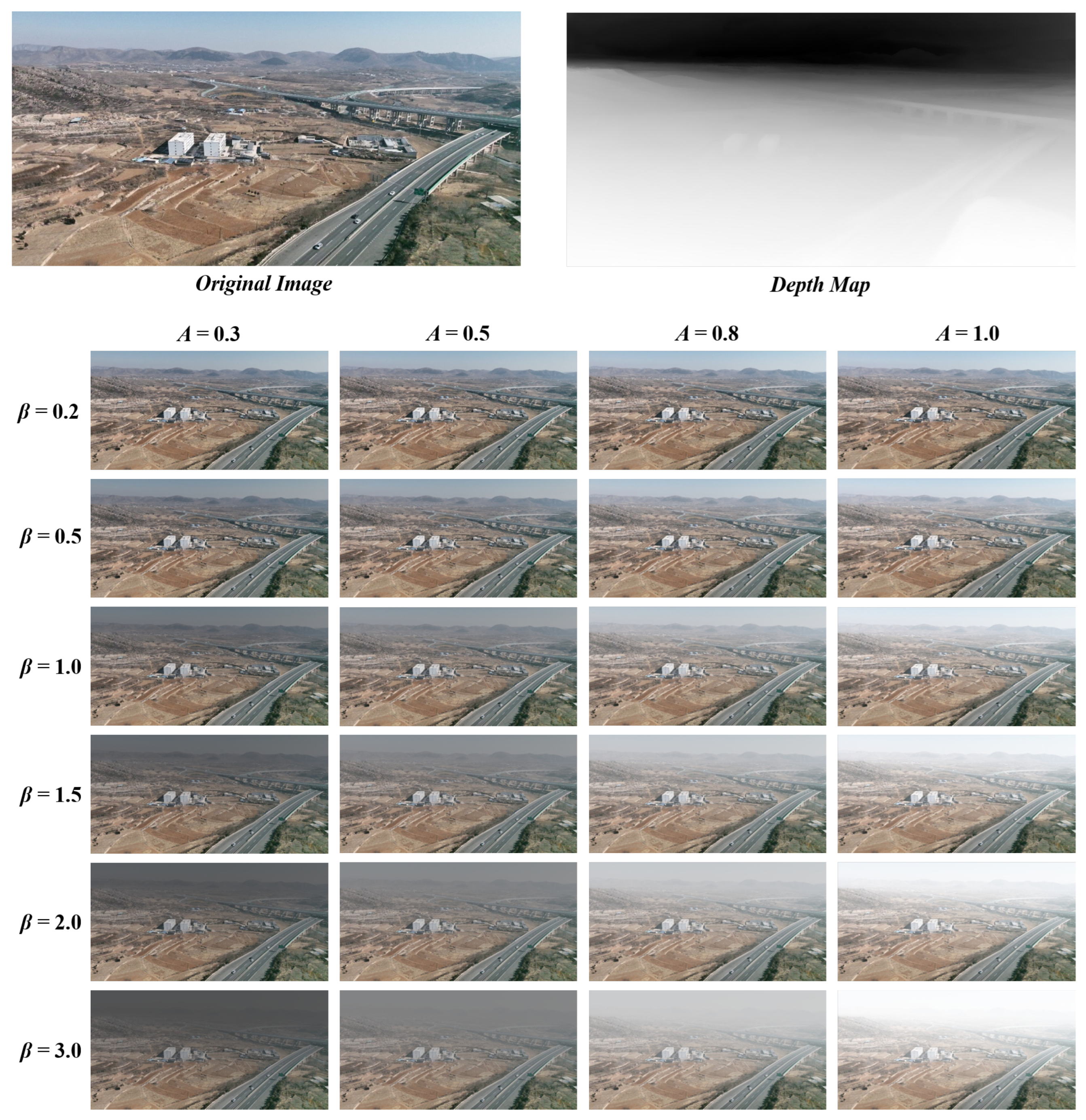
In order to achieve synthetic hazy pictures, it was necessary to manipulate the original images that were shot in ideal lighting conditions. At first, we needed to obtain the images’ depth maps. In this research, we decided to estimate the original image’s depth using Marigold [53]. Marigold is the SOTA depth estimation method which generates depth maps for input images via stable diffusion. It achieves excellent results in various scenarios, but due to its time-consuming nature, it was only suitable for the depth estimation task in the data processing stage of this study. Subsequently, the atmospheric scattering model in Equation (1) can be used to create various degrees of hazy images. In this study, we established the values for the global atmospheric light as and for the atmospheric scattering coefficient as . Figure 9 displays an example of the original image, depth map, and synthetic hazy images from the UAV-HAZE dataset. It can be clearly observed that as the global atmospheric light A increases, the image becomes brighter, while as the atmospheric scattering coefficient increases, the haze concentration in the image gradually intensifies. Additionally, the haze concentration in a single image varies significantly with depth, being sparser in the foreground and denser in the background, which aligns well with the real-world discipline and characteristics of long-range scenes. In summary, the UAV-HAZE dataset included 34,344 synthetic hazy images with their original images and depth maps. Furthermore, the UAV-HAZE also comprised approximately 400 real hazy images for testing in real-world environments.

Figure 9.
The example images in the UAV-HAZE dataset, including the original image, the depth map, and synthetic hazy images generated by the atmospheric scatting model.
4.3. Dataset Analysis
In order to assess the authenticity of our proposed dataset, we carried out user research that included comparing it with real-world hazy pictures as well as images from other hazy datasets. Specifically, we recruited a total of 25 participants, comprising 17 males and 8 females, for our research. Afterwards, we provided them with the images we collected, which included (i) ten random synthetic hazy images from our UAV-HAZE dataset, (ii) ten real-world hazy images downloaded from the Internet by searching “hazy images”, (iii) ten images from the SOTS-outdoor-hazy part in the RESIDE dataset [38], (iv) ten hazy images from the O-HAZE dataset in NTIRE 2018 [50,54], (v) ten hazy images from the NH-HAZE dataset [51], and (vi) ten hazy images from the Dense-Haze dataset [52]. A total of sixty images were provided to the participants in random order, and they were asked to rate their realness on a scale of 0 (fake) to 10 (real). We collected and analyzed the ratings for each category, and the results are summarized in Table 2.
Table 2.
Rating result of the research, including mean ratings (from 0 (fake) to 10 (real)) and standard deviation given by the participants.
Based on the results shown in Table 2, it is evident that our proposed dataset exhibited ratings that were more closely aligned with those of real-world hazy pictures in comparison to the other four hazy datasets. This indicated that the images in our dataset more closely resembled the distribution of haze in real-world scenarios. However, several participants mentioned that some of our images were overly dim, which was the main reason for the discrepancy in ratings compared to real hazy images.
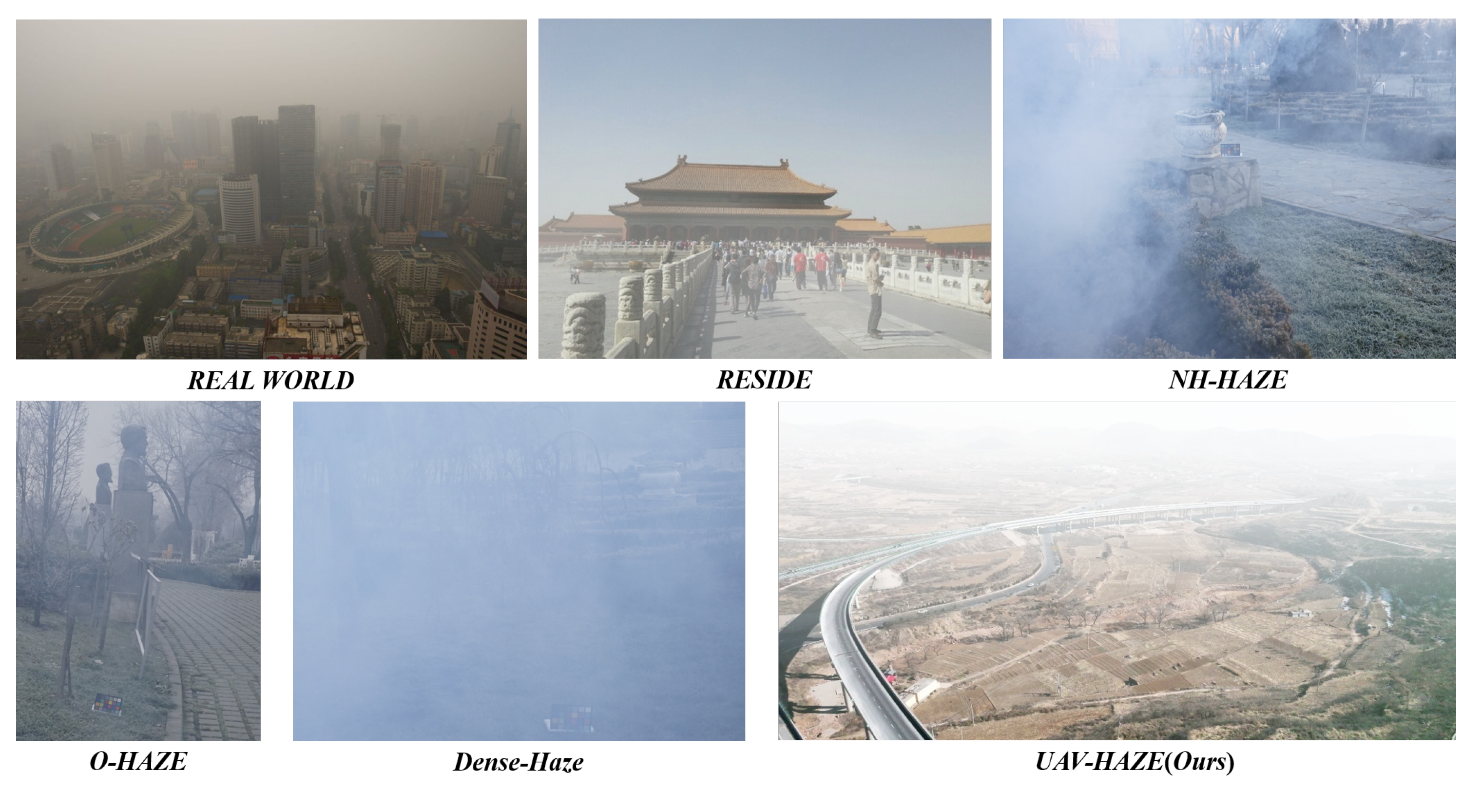
Figure 10 graphically illustrates the attributes of images in several hazy datasets. The RESIDE dataset applies a consistent blur filter to clear pictures, resulting in equally blurred images at both close and long distances. This introduces a notable disparity with real-world images. O-HAZE, NH-HAZE, and Dense-haze use a smoke generator to create real haze, indicating that these images are not artificially created but obtained from real photography. It is undeniable that the results do not entirely conform to the depth distribution observed in the real world but instead display a certain degree of randomness in their distribution. Conversely, our proposed UAV-HAZE dataset closely approximates the distribution of actual hazy photos, unlike other datasets. These pictures demonstrate that details and contours are not severely muted in close areas, while distant places are noticeably blurred because of the haze that has accumulated. This observation provides clear evidence that our dataset has a strong resemblance to real-world hazy photos, confirming the results presented in Table 2.
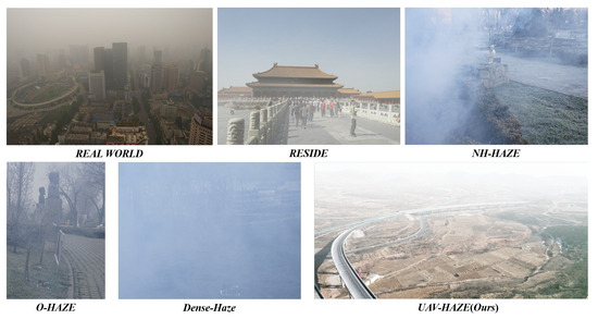
Figure 10.
Comparison of images from different datasets.
5. Experimental Results
This part involved conducting experiments on both synthetic and real images to verify the efficacy of our method in recovering long-range scenes.
5.1. Experimental Setup
- Operation environment: all experiments were based on the PyTorch library and ran on the Ubuntu 20.04 system, with an Intel® Xeon® Gold 6430 CPU and an RTX 4090 (24 GB) GPU;
- Evaluation metrics: This paper employed common metrics, the Peak Signal-to-Noise Ratio (PSNR) and Structural Similarity (SSIM) index, to quantitatively evaluate the dehazing performance of various methods [55]. Although the parameter results are not perfectly equal to the dehazing effectiveness, larger PSNR and SSIM values generally indicate better performance. The definitions of PSNR and SSIM are as follows:where represents the maximum possible value of the pixels in the image, typically 255, and stands for Mean Squared Error.where x and y are sliding windows of the two images, and are the means, while and are the standard deviation, is the covariance between x and y, and and are constants used for stabilizing the computation.Additionally, to further analyze the quality of the dehazed images obtained by our method, we employed the NIQE (Natural Image Quality Evaluator) [56] to quantify it from the data perspective. The NIQE, which incorporates statistical features of natural images, can provide evaluation results that are more consistent with human visual perception compared to the PSNR and SSIM.
- Parameters setting: The controllable factors in the MRDM were defined by setting the number of RDBs to two, while the weight coefficient in the loss function was set to 0.8, as explained in Section 3.1 and Section 3.4. During the training process, we started by randomly assigning initial weights to the network from a Gaussian distribution. Next, we used the Adam optimization algorithm [57], with a first momentum value of 0.9, a second momentum value of 0.999, and a weight decay of zero. The initial learning rate was set to . The policy of “poly” reduced it to a power of 0.9 and stopped it after 100,000 iterations.
5.2. Results on Synthetic Images
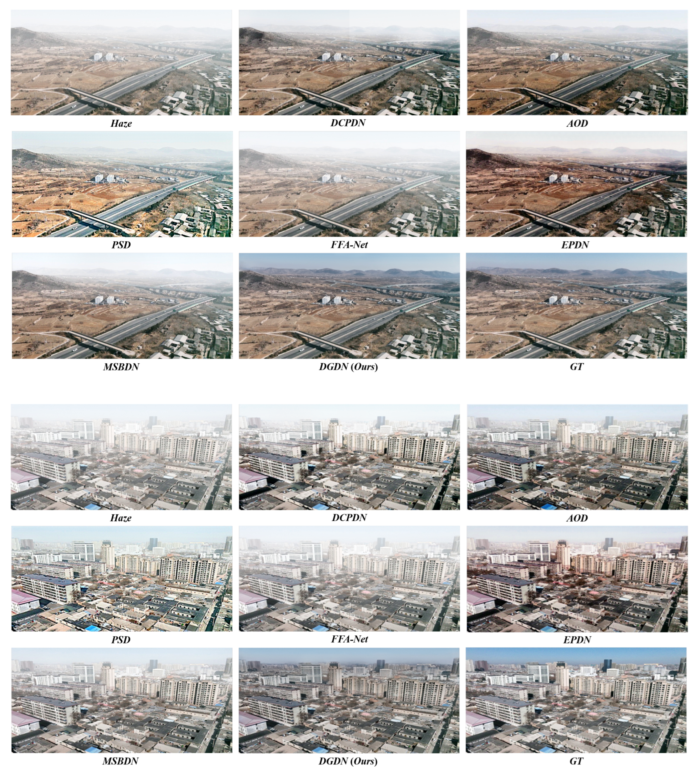
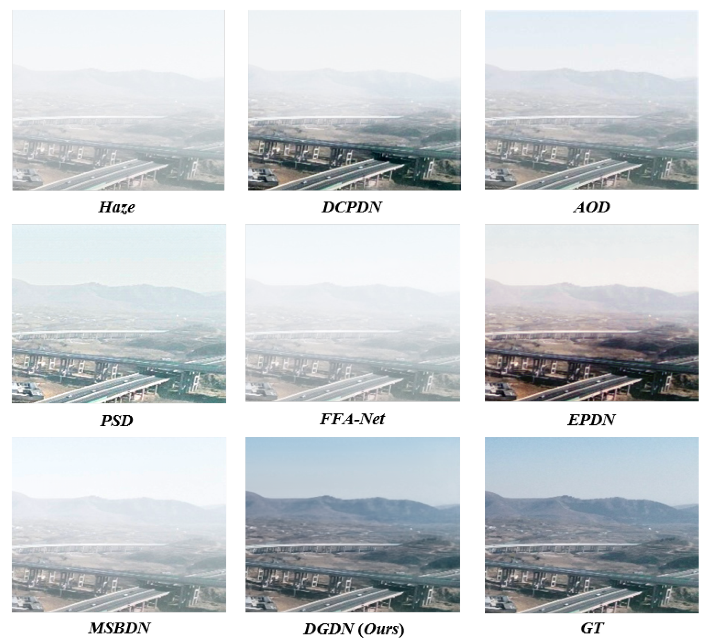
We randomly selected 50 images from the UAV-HAZE dataset for evaluating the dehazing results of SOTA dehazing methods, which included DCPDN [23], AOD [24], PSD [27], FFA-Net [28], EPDN [29], and MSBDN [31]. In order to clearly demonstrate the variation in the effects of long-range dehazing, we present a comparison of the results obtained by different dehazing methods on two images, as seen in Figure 11. These two images displayed a low-altitude oblique top perspective, which aligned with the long-range image described in Section 2.3. As the depth increased, the concentration of haze grew as well, resulting in clear visibility in nearby areas and decreased visibility in distant areas, which was exactly the scenario we wanted to deal with. For the first image, our method successfully restored the distant mountain area without chromatic aberration. In contrast, the SOTA methods were unsuccessful at effectively restoring the distant mountain area, resulting in persistent haziness. Moreover, EPDN [29] also produced very serious chromatic aberration. In conclusion, our method effectively achieved a more accurate restoration effect compared to the ground truth (GT). In the case of the second picture, our approach likewise attained the most optimal restoration result for distant buildings, effectively enhancing their delineation, a task that other SOTA methods were unable to achieve. Hence, the empirical findings unequivocally demonstrated that our method attained the best dehazing performance while handling long-range images.
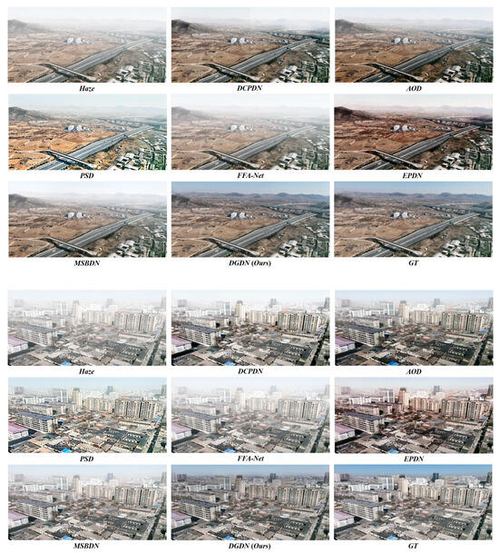
Figure 11.
The results on synthetic images in UAV-HAZE through different methods.
Additionally, we have precise data that substantiate our conclusions. Specifically, we calculated the average PSNR, SSIM, and NIQE for each method, as shown in Table 3. Compared to other SOTA dehazing approaches, it is evident that our approach obtained the highest values in PSNR and SSIM while the lowest one in NIQE, suggesting that it performed the best on long-range images and produced more pleasing results that aligned with human visual perception.
Table 3.
Comparison with SOTA methods using PSNR, SSIM, and NIQE on synthetic hazy images.
5.3. Results on Real-World Images
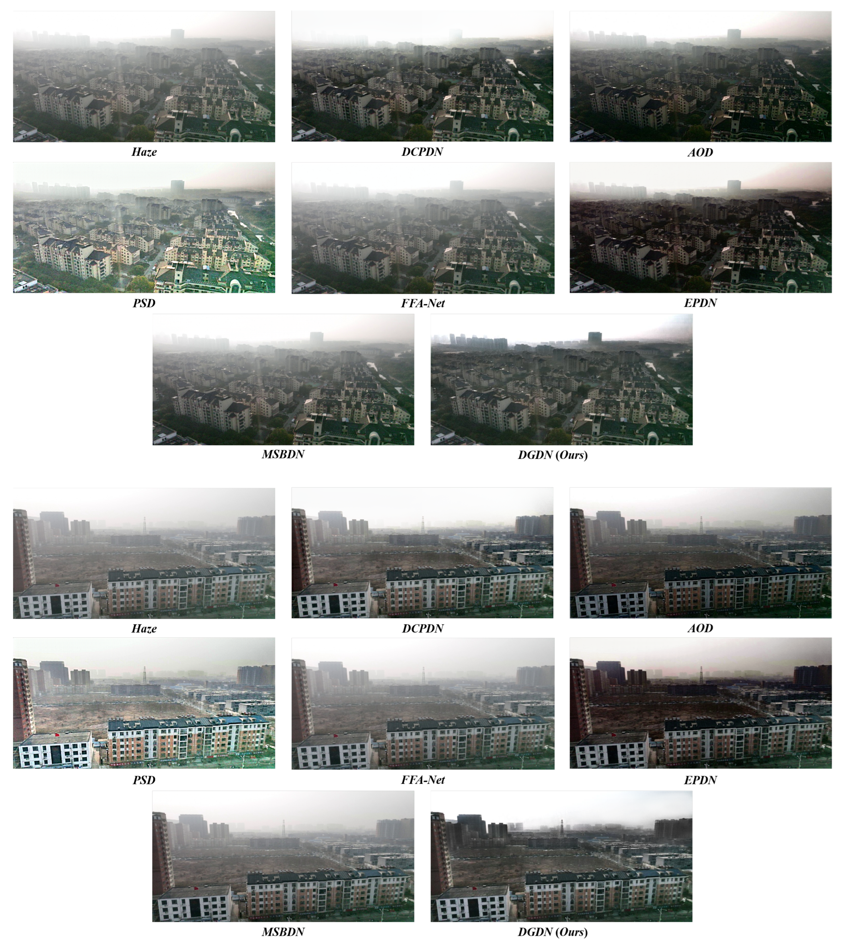
In order to assess the effectiveness of our method on real-world photos, we performed experiments using the real part of UAV-HAZE and compared its performance with other SOTA dehazing methods. Our method demonstrated exceptional performance on real images, as seen in Figure 12. The first picture reveals clear and distinct features of the structures nearby, but the distant buildings seem blurry, making it difficult to discern their exact outlines and intricate characteristics. Hence, in order to enhance the appearance, dehazing methods should be specifically focused on the remote areas. Other SOTA methods were unable to adequately restore the outlines of distant buildings, particularly in the group of buildings situated in the upper left corner. On the other hand, our method successfully brought back the remote areas, enabling a distinct representation of the outlines of distant buildings while maintaining the precise characteristics of buildings at medium and close distances. The second picture showcases a similar phenomenon, in which our methodology effectively reinstated the outlines and intricacies of some distant structures, an achievement that other SOTA methods were unable to accomplish. In summary, our approach was capable of achieving outstanding results in dehazing on real-world images, showcasing its ability to perform well on realistic datasets.
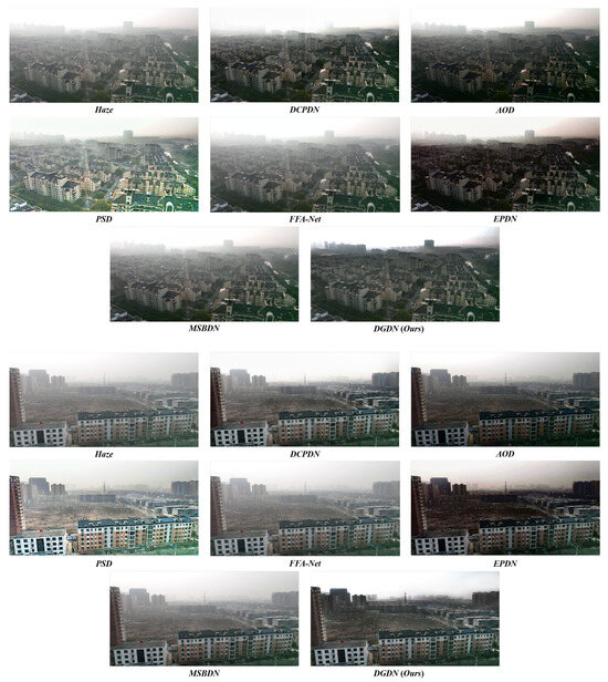
Figure 12.
The results on real-world images in UAV-HAZE through different methods.
6. Discussion
This section provides a three-fold analysis of our proposed method: first, we discuss the depth map obtained using various methods; second, we discuss the ablation experiment to emphasize the importance of the depth-guided attention module; and third, we discuss the comparative experiment to demonstrate the benefits of our method over other SOTA methods.
6.1. Discussion of the Depth Map
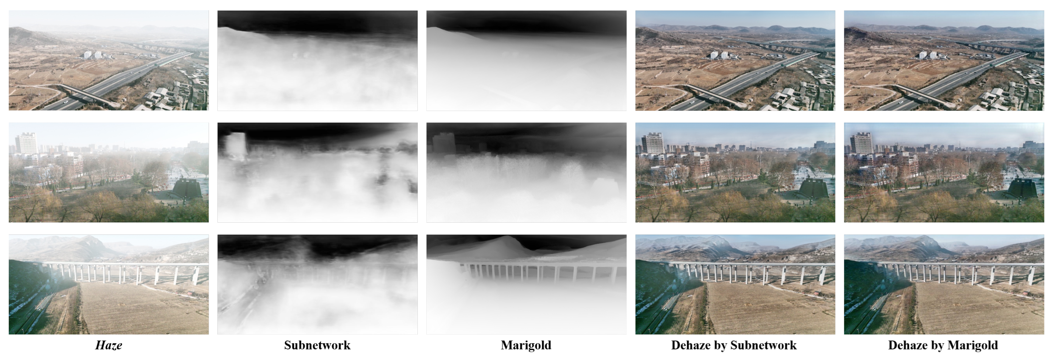
This section primarily focuses on contrasting the depth estimation subnetwork used in this article with the results achieved by Marigold [53] utilized in the UAV-HAZE dataset. Simultaneously, it elucidates the correlation between the distribution of haze concentration in the hazy image and the depth map, in order to substantiate the rationale supporting using depth information to direct the dehazing procedure, especially for long-range images.
Figure 13 displays the depth maps acquired by the depth estimation subnetwork presented in this article and Marigold [53]. Within our depth prediction subnetwork, each MRDM consisted of two RDBs, and each RDB had five individual dense layers. In Marigold [53], we assigned a value of 10 to both the “denoise steps” and “ensemble size” parameters for every single image. This means that we conducted 10 denoising inference steps for each prediction and then calculated the average result of these 10 predictions as the final output. Figure 13 clearly demonstrates that Marigold [53] outperformed in depth estimation, providing more distinct outlines and features. However, our depth estimation subnetwork also predicted similar depth distribution results, although it missed certain specific details. Nevertheless, the dehazing impact was not dependent on this factor, as seen in Figure 13, which shows that the use of these two depth maps produced almost identical dehazing performance. However, when considering the aspect of time, our approach had a significant benefit. Table 4 displays the duration required for the three pictures in Figure 13 on the device mentioned in Section 5.1. The depth prediction subnetwork had a processing time of just 0.035 s, whereas Marigold [53] took 6.23 s, which amounted to a difference factor of approximately 180. The proposed approach effectively decreased the time required while maintaining the dehazing effect, making it well suited for platforms with low processing capabilities, such as UAV.

Figure 13.
The depth maps and dehazing results by the proposed depth prediction subnetwork and Marigold [53].
Table 4.
The time cost of different methods for depth prediction.
Figure 13 shows the link between the distribution of haze concentration and the depth map on the long-range images. The hazy image exhibits an uneven distribution of haze densities. The bottom portion exhibits a less dense fog, allowing for clearer visibility of the image’s features. In contrast, the top portion is characterized by a denser fog, resulting in a whitish, hazy region. The depth information corresponds to the distance to things, with light-colored regions in the depth map indicating nearby objects and dark-colored portions indicating distant ones. The dark regions in the depth map accurately correspond to the places with the highest density of fog in the foggy picture, namely the hazy regions. This illustrates the strong association between depth information and the process of removing haze from long-range images. Moreover, our dehazing results confirm the accuracy of this correlation.
6.2. Discussion of the Ablation Experiment
In order to assess the efficacy of the DGAM, we performed ablation experiments as shown in Table 5. The first row in Table 5 signifies the results obtained solely using the haze removal subnetwork without incorporating depth information as baseline, thereby validating the efficacy of depth information in long-range dehazing. The second row in Table 5 introduces depth information but does not utilize the DGAM when dehazing, thus verifying the effectiveness of the DGAM. The results achieved by the proposed DGDN approach are shown in the third row of Table 5.
Table 5.
The results of the ablation experiment.
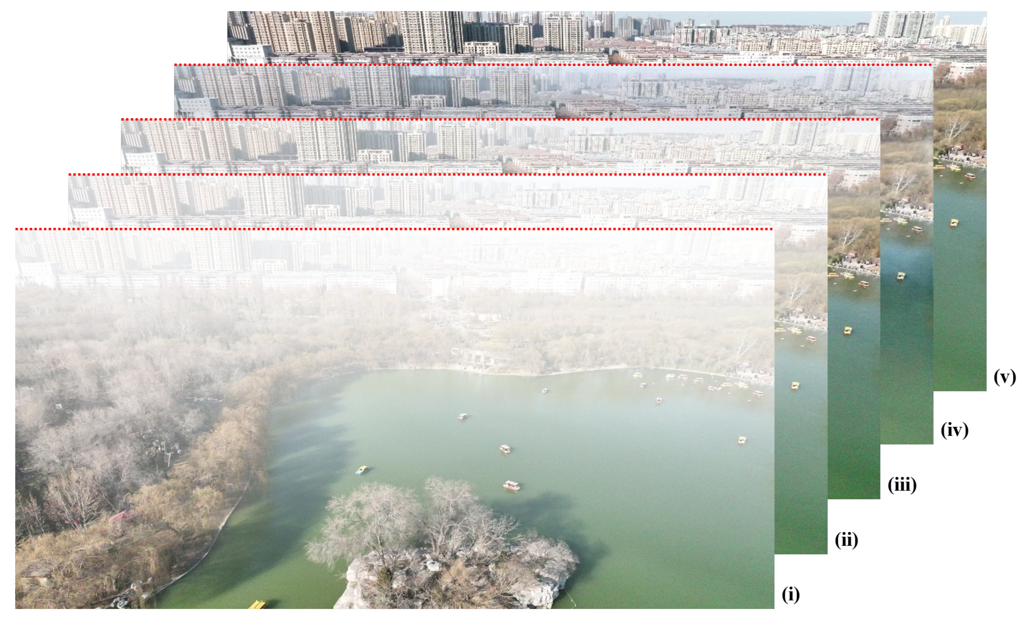
Table 5 demonstrates that our DGDN outperformed other methods in the ablation studies, emphasizing the beneficial impact of the DGAM’s depth-guided attention methodology. To visually demonstrate the differences between these baselines, we plotted them in Figure 14. It shows the results obtained by the baseline and variants and the hazy images and ground truth: (i) original hazy image, (ii) the haze removal subnetwork only, (iii) haze removal subnetwork with depth information (without DGAM), (iv) our proposed DGAM method, (v) ground truth. Furthermore, the focus of this ablation experiment was on the dehazing effect in the long-range part. Therefore, we stacked these images to highlight more prominently the dehazing effect achieved by different methods in the long-range area, resulting in a clearer and more pronounced contrast.
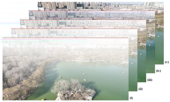
Figure 14.
The visualization of the ablation experiment for depth information and the DGAM. Since this experiment focused more on the comparison of long-range dehazing performance, we stacked the images and used red dashed lines to distinguish key areas for an obvious contrast by different methods. From front to back: (i) original hazy image, (ii) haze removal subnetwork only, (iii) haze removal subnetwork with depth information (without DGAM), (iv) our proposed DGAM method, (v) ground truth. Our method achieves the best dehazing performance in the long-range area.
From Figure 14, it can be observed that the results obtained when only using the haze removal subnetwork had a poor dehazing effect in the long-range area (compared with (i) and (ii) in Figure 14). After introducing depth information, there was a slight improvement in the dehazing effect, but the area still appeared blurry, indicating a noticeable impact from the haze (compared with (ii) and (iii) in Figure 14). By applying the DGAM, there was a significant improvement in the dehazing effect, with clear texture structures visible in the long-range area. The image representation also appeared more natural. This indicated the excellent performance of our proposed method in long-range dehazing (compared with (ii), (iii), and (iv) in Figure 14). However, it is regrettable that the long-range area typically has a denser haze density, which means that the degradation caused by hazy environments is more severe. Consequently, there was still a little difference between the dehazed images produced by our approach and the actual reference pictures. This discrepancy is an area that requires further improvement in future iterations, as seen in (iv) and (v) in Figure 14.
6.3. Discussion of the Comparative Experiment
This section discusses the experimental results obtained in Section 5.2 and Section 5.3, demonstrating the benefits of our suggested approach in long-range dehazing.
6.3.1. Discussion on Synthetic Images
In order to effectively showcase the dehazing performance of our suggested methodology in long-range regions, we extracted and enlarged relevant portions of those pictures, as shown in Figure 15. It displays the experiment’s visualization on synthetic images using the SOTA methods mentioned in Section 5.2. It is clear that our approach produced the most effective dehazing impact.

Figure 15.
The dehazed long-range areas of synthetic images. Pictures are from Figure 11.
Specifically, in Figure 15, our method demonstrated excellent dehazing results for the mid-to-long-range highway and the distant mountains. The contour lines and specific details are clearly visible, and the restored image is closer to the ground truth in terms of color. Additionally, the color rendition of the sky is also more accurate. In contrast, other SOTA approaches such as AOD [24], PSD [27], FFA-Net [28], and MSBDN [31] exhibited poor dehazing performance in that area. They failed to thoroughly dehaze the highway area, let alone the distant mountains. As for DCPDN [23] and EPDN [29], they indeed showcased impressive dehazing performance in the highway area. However, their performance notably suffered when handling distant mountains. Additionally, both of them fell short of delivering satisfactory restoration in the sky area. Furthermore, the image obtained by EPDN [29] exhibited severe color cast issues in the overall image, with several overly dark regions, resulting in the loss of crucial details such as texture information. On the other hand, our approach successfully overcame these issues.
6.3.2. Discussion on Real-World Images
We applied the methodology illustrated in Figure 15 to analyze the dehazing results obtained on real-world images in Figure 16. To more effectively analyze the discrepancies in outcomes produced by different methods, we magnified our focus on the distant regions, where the distinction between nearby and distant buildings becomes apparent.
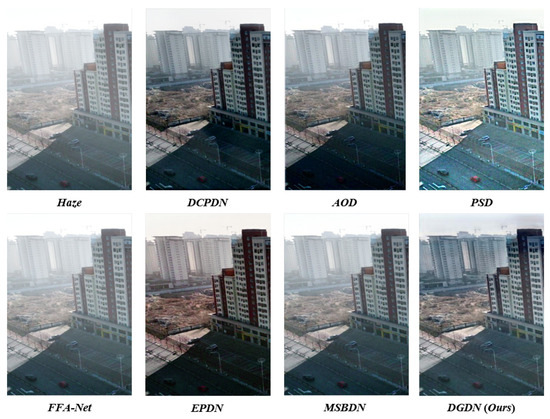
Figure 16.
The dehazed long-range areas of real-world images.
When applied to real-world circumstances, the SOTA approaches, namely, DCPDN [23], AOD [24], EPDN [29], FFA-Net [28], and MSBDN [31], demonstrated the same issues noted earlier. For instance, while these methods achieved acceptable results when processing nearby buildings, with EPDN [29] displaying sharper performance, they still failed to produce satisfactory outcomes when dealing with distant buildings, leaving them in the hazy state. PSD [27] performed well on real-world images, with brighter visuals, due to the particular transfer from synthetic to real world. However, it also failed to completely dehaze distant buildings, and there was obvious noise in the image. In contrast, our method effectively restored the distant buildings, revealing clear contours and details. It is also evident that both AOD [24] and EPDN [29] created large areas of excessive darkness in the shadows of the buildings, resulting in a significant loss of detail. This phenomenon is particularly prominent in Figure 12, where both methods displayed a severe color bias. In contrast, our method achieved better color reproduction. However, our method may produce slight artifacts along the edges when processing some images, such as the sky area in Figure 16, which is an aspect that requires further optimization in our future work.
6.4. Discussion of the Training Sets
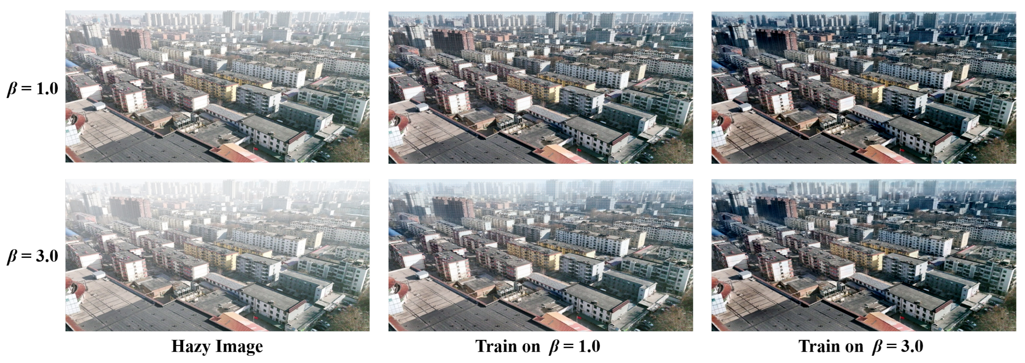
As mentioned earlier, the UAV-HAZE dataset contains synthetic hazy images of various densities, which can cover diverse application scenarios. This subsection aims to study the impact of different haze densities in the training sets on the model’s dehazing results, thus investigating the model’s generalization performance. To this end, we selected two different training sets: synthetic images with in UAV-HAZE, representing a light haze, and synthetic images with representing a thick haze. Subsequently, we trained the model on the two training sets until convergence and tested their dehazing performance under both densities. The results are shown in Figure 17, where the first row represents images with a light haze (), and the second row represents images with a thick haze (). From left to right, Figure 17 displays the synthetic hazy images in the UAV-HAZE dataset, the dehazing results of the model trained on the dataset, and dehazing results of the model trained on the one. The obtained results were consistent with human intuition. It can be seen that both models achieved good dehazing results in their respective fields. But obviously, the model trained on the light-haze dataset () struggled to thoroughly dehaze the thick-haze images (), with distant regions still remaining blurred. In contrast, the model trained on the thick-haze dataset () could easily restore clear images when dealing with light-haze images (). However, it should be noted that although the distant regions seemed to have clearer details, their brightness also decreased significantly, which is a phenomenon of excessive dehazing according to CAP [19].
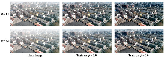
Figure 17.
The dehazing performance from different training sets. The first row is the synthetic image with in the UAV-HAZE dataset, which has a relatively light haze, while the second row is its counterpart with , which has a relatively thicker haze. From left to right are: the synthetic hazy image, the dehazing results of the model trained on the training set with , and the dehazing results of the model trained on the training set with .
Therefore, it can be concluded that the model trained on the thick-haze training set had good downward compatibility and could handle scenes with relatively lighter haze densities, while the model trained on the light-haze training set could not handle thicker-haze scenes well. However, the model trained on the thick-haze training set may suffer from excessive dehazing and lead to a brightness reduction when processing different scenes, indicating its limitations. In a more ideal condition, training models with different levels of haze densities to distinguish them can achieve optimal results in their respective fields.
6.5. Discussion of the Time Cost
Time cost is also an important aspect of evaluating the algorithms. In this section, we compared the time cost between the proposed method and other SOTA dehazing algorithms, and the specific results are shown in Table 6. It can be seen that our proposed method was not the fastest. With its simple network structure, AOD [24] outperformed other methods in terms of time cost and took the lead. However, our method was still on the same order of magnitude compared with other methods, and there was no significant lag. As our proposed method was designed for long-range scenes, we expected to obtain faster results to adapt to platforms with limited computing sources. Therefore, we attempted to reduce the dense layers in the depth prediction subnetwork from five to three, and the network speed was improved by nearly 30%, but this came at the cost of sacrificing some defogging results. It must be acknowledged that our method does not have an advantage in speed at present, which is also one of the directions for optimization in the future.
Table 6.
Time cost for different dehazing methods.
7. Conclusions
In this article, we proposed the depth-guided dehazing network, specifically designed for long-range scenes. At first, we introduced the atmospheric scattering model of the haze environment and further analyzed the impact of different camera perspectives on the imaging characteristics of hazy scenes. As a result, we defined long-range scenes as those in which significant depth variations within a single image lead to corresponding changes in haze density. To address the dehazing challenges posed by such scenes, we introduced our method, which comprised three main components: (i) a depth prediction subnetwork, (ii) a haze removal subnetwork, and (iii) a depth-guided attention module. This network leveraged depth information to guide the dehazing process, enabling excellent dehazing performance in long-range scenarios.
Then, addressing the scarcity and dispersal of long-range images in existing dehazing datasets, we introduced the UAV-HAZE dataset. This dataset comprised exclusively long-range photos captured by UAVs, encompassing diverse scenarios. It included 34,334 synthetic hazy images with varying concentrations and brightness levels, as well as nearly 400 real-world hazy images, serving as a valuable resource for training and evaluating long-range scene’s dehazing tasks. On the UAV-HAZE dataset, we carried out ablation experiments and comparison experiments using several SOTA approaches, comprehensively showcasing the effectiveness of our suggested method for dehazing long-range scenes. Looking ahead, we will continue to focus on addressing the degradation of depth prediction in hazy images, aiming to achieve better dehazing results in long-range scenes.
Author Contributions
Conceptualization, Y.W. and C.F.; methodology, Y.W. and J.Z.; formal analysis, Y.W. and J.Z.; investigation, Y.W. and J.Z.; resources, C.F.; data curation, Y.W.; writing—original draft preparation, Y.W.; writing—review and editing, J.Z., L.Y. and C.F.; visualization, Y.W.; supervision, C.F.; project administration, Y.W.; funding acquisition, C.F. All authors have read and agreed to the published version of the manuscript.
Funding
This work was funded by the Natural Science Foundation of Shanghai under grant no. 20ZR1460100.
Data Availability Statement
The code and UAV-HAZE datasets are available at https://github.com/wangyihu1215/DGDN (accessed on 3 June 2024).
Conflicts of Interest
The authors declare no conflicts of interest.
Abbreviations
| UAV | Unmanned aerial vehicle |
| DGDN | Depth-guided dehazing network |
| RDB | Residual dense block |
| MRDM | Multiple residual dense module |
| DGAM | Depth-guided attention module |
| DCP | Dark Channel Prior |
| CAP | Color Attenuation Prior |
| RGB | Red, green, blue |
| HSV | Hue, saturation, value |
| DCPDN | Densely Connected Pyramid Dehazing Network |
| AOD-Net | All-In-One Network |
| GAN | Generative Adversarial Network |
| FFA-Net | Feature Fusion Attention Network |
| EPDN | Enhanced Pix2pix Dehazing Network |
| CycleGAN | Cycle Generative Adversarial Network |
| MSBDN | Multiscale boosted dehazing network |
| MSE | Mean Squared Error |
| PSD | Principled Synthetic-to-real Dehazing |
| DDRB | Depth-wise Dilated Residual Block |
| SELU | Scaled Exponential Linear Unit |
| CNN | Convolutional neural network |
| PSNR | Peak Signal-to-Noise Ratio |
| SSIM | Structural Similarity |
| SOTA | State of the art |
| GT | Ground truth |
| FPS | Frames per second |
References
- Fan, B.; Li, Y.; Zhang, R.; Fu, Q. Review on the technological development and application of UAV systems. Chin. J. Electron. 2020, 29, 199–207. [Google Scholar] [CrossRef]
- Hardin, P.J.; Jensen, R.R. Small-scale unmanned aerial vehicles in environmental remote sensing: Challenges and opportunities. GISci. Remote Sens. 2011, 48, 99–111. [Google Scholar] [CrossRef]
- Sahu, G.; Seal, A.; Bhattacharjee, D.; Nasipuri, M.; Brida, P.; Krejcar, O. Trends and prospects of techniques for haze removal from degraded images: A survey. IEEE Trans. Emerg. Top. Comput. Intell. 2022, 6, 762–782. [Google Scholar] [CrossRef]
- Liu, J.; Wang, S.; Wang, X.; Ju, M.; Zhang, D. A review of remote sensing image dehazing. Sensors 2021, 21, 3926. [Google Scholar] [CrossRef]
- Agrawal, S.C.; Jalal, A.S. A comprehensive review on analysis and implementation of recent image dehazing methods. Arch. Comput. Methods Eng. 2022, 29, 4799–4850. [Google Scholar] [CrossRef]
- Ancuti, C.O.; Ancuti, C.; Vasluianu, F.A.; Timofte, R. NTIRE 2021 nonhomogeneous dehazing challenge report. In Proceedings of the IEEE/CVF Conference on Computer Vision and Pattern Recognition, Nashville, TN, USA, 19–25 June 2021; pp. 627–646. [Google Scholar]
- Khan, H.; Xiao, B.; Li, W.; Muhammad, N. Recent advancement in haze removal approaches. Multimed. Syst. 2022, 28, 687–710. [Google Scholar] [CrossRef]
- Sharma, T.; Shah, T.; Verma, N.K.; Vasikarla, S. A Review on Image Dehazing Algorithms for Vision based Applications in Outdoor Environment. In Proceedings of the 2020 IEEE Applied Imagery Pattern Recognition Workshop (AIPR), Washington, DC, USA, 13–15 October 2020; pp. 1–13. [Google Scholar]
- Juneja, A.; Kumar, V.; Singla, S.K. A systematic review on foggy datasets: Applications and challenges. Arch. Comput. Methods Eng. 2022, 29, 1727–1752. [Google Scholar] [CrossRef]
- Vaswani, A.; Shazeer, N.; Parmar, N.; Uszkoreit, J.; Jones, L.; Gomez, A.N.; Kaiser, Ł.; Polosukhin, I. Attention is all you need. Adv. Neural Inf. Process. Syst. 2017, 30, 5998–6008. [Google Scholar]
- Nayar, S.K.; Narasimhan, S.G. Vision in bad weather. In Proceedings of the Seventh IEEE International Conference on Computer Vision, Kerkyra, Greece, 20–27 September 1999; Volume 2, pp. 820–827. [Google Scholar]
- Narasimhan, S.G.; Nayar, S.K. Chromatic framework for vision in bad weather. In Proceedings of the IEEE Conference on Computer Vision and Pattern Recognition. CVPR 2000 (Cat. No. PR00662), Hilton Head, SA, USA, 12–15 June 2000; Volume 1, pp. 598–605. [Google Scholar]
- McCartney, E.J. Optics of the Atmosphere: Scattering by Molecules and Particles; Wiley: New York, NY, USA, 1976. [Google Scholar]
- Wang, W.; Chang, F.; Ji, T.; Wu, X. A fast single-image dehazing method based on a physical model and gray projection. IEEE Access 2018, 6, 5641–5653. [Google Scholar] [CrossRef]
- Vazquez-Corral, J.; Finlayson, G.D.; Bertalmío, M. Physical-based optimization for non-physical image dehazing methods. Opt. Express 2020, 28, 9327–9339. [Google Scholar] [CrossRef]
- Wang, J.; Lu, K.; Xue, J.; He, N.; Shao, L. Single image dehazing based on the physical model and MSRCR algorithm. IEEE Trans. Circuits Syst. Video Technol. 2017, 28, 2190–2199. [Google Scholar] [CrossRef]
- He, K.; Sun, J.; Tang, X. Single image haze removal using dark channel prior. IEEE Trans. Pattern Anal. Mach. Intell. 2010, 33, 2341–2353. [Google Scholar]
- Wang, J.B.; He, N.; Zhang, L.L.; Lu, K. Single image dehazing with a physical model and dark channel prior. Neurocomputing 2015, 149, 718–728. [Google Scholar] [CrossRef]
- Zhu, Q.; Mai, J.; Shao, L. A fast single image haze removal algorithm using color attenuation prior. IEEE Trans. Image Process. 2015, 24, 3522–3533. [Google Scholar]
- Berman, D.; treibitz, T.; Avidan, S. Non-Local Image Dehazing. In Proceedings of the IEEE Conference on Computer Vision and Pattern Recognition (CVPR), Las Vegas, NV, USA, 26 June–1 July 2016. [Google Scholar]
- Cai, B.; Xu, X.; Jia, K.; Qing, C.; Tao, D. Dehazenet: An end-to-end system for single image haze removal. IEEE Trans. Image Process. 2016, 25, 5187–5198. [Google Scholar] [CrossRef]
- Ren, W.; Liu, S.; Zhang, H.; Pan, J.; Cao, X.; Yang, M.H. Single image dehazing via multi-scale convolutional neural networks. In Proceedings of the Computer Vision–ECCV 2016: 14th European Conference, Amsterdam, The Netherlands, 11–14 October 2016; Springer: Berlin/Heidelberg, Germany, 2016. Proceedings, Part II 14. pp. 154–169. [Google Scholar]
- Zhang, H.; Patel, V.M. Densely connected pyramid dehazing network. In Proceedings of the IEEE Conference on Computer Vision and Pattern Recognition, Salt Lake City, UT, USA, 18–23 June 2018; pp. 3194–3203. [Google Scholar]
- Li, B.; Peng, X.; Wang, Z.; Xu, J.; Feng, D. Aod-net: All-in-one dehazing network. In Proceedings of the IEEE International Conference on Computer Vision, Venice, Italy, 22–29 October 2017; pp. 4770–4778. [Google Scholar]
- Zhu, H.; Cheng, Y.; Peng, X.; Zhou, J.T.; Kang, Z.; Lu, S.; Fang, Z.; Li, L.; Lim, J.H. Single-image dehazing via compositional adversarial network. IEEE Trans. Cybern. 2019, 51, 829–838. [Google Scholar] [CrossRef]
- Yang, Y.; Wang, C.; Liu, R.; Zhang, L.; Guo, X.; Tao, D. Self-augmented unpaired image dehazing via density and depth decomposition. In Proceedings of the IEEE/CVF Conference on Computer Vision and Pattern Recognition, New Orleans, LA, USA, 18–24 June 2022; pp. 2037–2046. [Google Scholar]
- Chen, Z.; Wang, Y.; Yang, Y.; Liu, D. PSD: Principled synthetic-to-real dehazing guided by physical priors. In Proceedings of the IEEE/CVF Conference on Computer Vision and Pattern Recognition, Nashville, TN, USA, 19–25 June 2021; pp. 7180–7189. [Google Scholar]
- Qin, X.; Wang, Z.; Bai, Y.; Xie, X.; Jia, H. FFA-Net: Feature fusion attention network for single image dehazing. In Proceedings of the AAAI Conference on Artificial Intelligence, New York, NY, USA, 7–12 February 2020; Volume 34, pp. 11908–11915. [Google Scholar]
- Qu, Y.; Chen, Y.; Huang, J.; Xie, Y. Enhanced pix2pix dehazing network. In Proceedings of the IEEE/CVF Conference on Computer Vision and Pattern Recognition, Long Beach, CA, USA, 16–17 June 2019; pp. 8160–8168. [Google Scholar]
- Engin, D.; Genç, A.; Kemal Ekenel, H. Cycle-dehaze: Enhanced cyclegan for single image dehazing. In Proceedings of the IEEE Conference on Computer Vision and Pattern Recognition Workshops, Salt Lake City, UT, USA, 18–22 June 2018; pp. 825–833. [Google Scholar]
- Dong, H.; Pan, J.; Xiang, L.; Hu, Z.; Zhang, X.; Wang, F.; Yang, M.H. Multi-scale boosted dehazing network with dense feature fusion. In Proceedings of the IEEE/CVF Conference on Computer Vision and Pattern Recognition, Seattle, WA, USA, 13–19 June 2020; pp. 2157–2167. [Google Scholar]
- Li, L.; Dong, Y.; Ren, W.; Pan, J.; Gao, C.; Sang, N.; Yang, M.H. Semi-supervised image dehazing. IEEE Trans. Image Process. 2019, 29, 2766–2779. [Google Scholar] [CrossRef]
- Shao, Y.; Li, L.; Ren, W.; Gao, C.; Sang, N. Domain adaptation for image dehazing. In Proceedings of the IEEE/CVF Conference on Computer Vision and Pattern Recognition, Seattle, WA, USA, 13–19 June 2020; pp. 2808–2817. [Google Scholar]
- Han, W.; Zhu, H.; Qi, C.; Li, J.; Zhang, D. High-resolution representations network for single image dehazing. Sensors 2022, 22, 2257. [Google Scholar] [CrossRef]
- Yu, J.; Liang, D.; Hang, B.; Gao, H. Aerial image dehazing using reinforcement learning. Remote Sens. 2022, 14, 5998. [Google Scholar] [CrossRef]
- Kulkarni, A.; Murala, S. Aerial Image Dehazing With Attentive Deformable Transformers. In Proceedings of the IEEE/CVF Winter Conference on Applications of Computer Vision (WACV), Waikoloa, HI, USA, 2–7 January 2023; pp. 6305–6314. [Google Scholar]
- Mehta, A.; Sinha, H.; Mandal, M.; Narang, P. Domain-aware unsupervised hyperspectral reconstruction for aerial image dehazing. In Proceedings of the IEEE/CVF Winter Conference on Applications of Computer Vision, Virtual, 5–9 January 2021; pp. 413–422. [Google Scholar]
- Li, B.; Ren, W.; Fu, D.; Tao, D.; Feng, D.; Zeng, W.; Wang, Z. Benchmarking Single-Image Dehazing and Beyond. IEEE Trans. Image Process. 2019, 28, 492–505. [Google Scholar] [CrossRef]
- Huang, B.; Zhi, L.; Yang, C.; Sun, F.; Song, Y. Single Satellite Optical Imagery Dehazing using SAR Image Prior Based on conditional Generative Adversarial Networks. In Proceedings of the IEEE/CVF Winter Conference on Applications of Computer Vision (WACV), Snowmass Village, CO, USA, 1–5 March 2020. [Google Scholar]
- Zhang, Y.; Tian, Y.; Kong, Y.; Zhong, B.; Fu, Y. Residual dense network for image super-resolution. In Proceedings of the IEEE Conference on Computer Vision and Pattern Recognition, Salt Lake City, UT, USA, 18–23 June 2018; pp. 2472–2481. [Google Scholar]
- Huang, G.; Liu, Z.; Van Der Maaten, L.; Weinberger, K.Q. Densely connected convolutional networks. In Proceedings of the IEEE Conference on Computer Vision and Pattern Recognition, Honolulu, HI, USA, 21–26 July 2017; pp. 4700–4708. [Google Scholar]
- He, K.; Zhang, X.; Ren, S.; Sun, J. Deep residual learning for image recognition. In Proceedings of the IEEE Conference on Computer Vision and Pattern Recognition, Las Vegas, NV, USA, 27–30 June 2016; pp. 770–778. [Google Scholar]
- Hu, X.; Zhu, L.; Wang, T.; Fu, C.W.; Heng, P.A. Single-image real-time rain removal based on depth-guided non-local features. IEEE Trans. Image Process. 2021, 30, 1759–1770. [Google Scholar] [CrossRef]
- Howard, A.G.; Zhu, M.; Chen, B.; Kalenichenko, D.; Wang, W.; Weyand, T.; Andreetto, M.; Adam, H. Mobilenets: Efficient convolutional neural networks for mobile vision applications. arXiv 2017, arXiv:1704.04861. [Google Scholar]
- Klambauer, G.; Unterthiner, T.; Mayr, A.; Hochreiter, S. Self-normalizing neural networks. Adv. Neural Inf. Process. Syst. 2017, 30, 972–981. [Google Scholar]
- Huang, S.C.; Chen, B.H.; Wang, W.J. Visibility restoration of single hazy images captured in real-world weather conditions. IEEE Trans. Circuits Syst. Video Technol. 2014, 24, 1814–1824. [Google Scholar] [CrossRef]
- Barron, J.T. A general and adaptive robust loss function. In Proceedings of the IEEE/CVF Conference on Computer Vision and Pattern Recognition, Long Beach, CA, USA, 16–17 June 2019; pp. 4331–4339. [Google Scholar]
- Zeiler, M.D.; Fergus, R. Visualizing and understanding convolutional networks. In Proceedings of the Computer Vision–ECCV 2014: 13th European Conference, Zurich, Switzerland, 6–12 September 2014; Springer: Berlin/Heidelberg, Germany, 2014. Proceedings, Part I 13. pp. 818–833. [Google Scholar]
- Simonyan, K.; Zisserman, A. Very deep convolutional networks for large-scale image recognition. arXiv 2014, arXiv:1409.1556. [Google Scholar]
- Ancuti, C.O.; Ancuti, C.; Timofte, R.; De Vleeschouwer, C. O-haze: A dehazing benchmark with real hazy and haze-free outdoor images. In Proceedings of the IEEE Conference on Computer Vision and Pattern Recognition Workshops, Salt Lake City, UT, USA, 18–23 June 2018; pp. 754–762. [Google Scholar]
- Ancuti, C.O.; Ancuti, C.; Timofte, R. NH-HAZE: An image dehazing benchmark with non-homogeneous hazy and haze-free images. In Proceedings of the IEEE/CVF Conference on Computer Vision and Pattern Recognition Workshops, Seattle, WA, USA, 13–19 June 2020; pp. 444–445. [Google Scholar]
- Ancuti, C.O.; Ancuti, C.; Sbert, M.; Timofte, R. Dense-haze: A benchmark for image dehazing with dense-haze and haze-free images. In Proceedings of the 2019 IEEE International Conference on Image Processing (ICIP), Taipei, Taiwan, 22–25 September 2019; pp. 1014–1018. [Google Scholar]
- Ke, B.; Obukhov, A.; Huang, S.; Metzger, N.; Daudt, R.C.; Schindler, K. Repurposing diffusion-based image generators for monocular depth estimation. arXiv 2023, arXiv:2312.02145. [Google Scholar]
- Ancuti, C.; Ancuti, C.O.; Timofte, R. Ntire 2018 challenge on image dehazing: Methods and results. In Proceedings of the IEEE Conference on Computer Vision and Pattern Recognition Workshops, Salt Lake City, UT, USA, 18–23 June 2018; pp. 891–901. [Google Scholar]
- Wang, Z.; Bovik, A.C.; Sheikh, H.R.; Simoncelli, E.P. Image quality assessment: From error visibility to structural similarity. IEEE Trans. Image Process. 2004, 13, 600–612. [Google Scholar] [CrossRef]
- Mittal, A.; Soundararajan, R.; Bovik, A.C. Making a “completely blind” image quality analyzer. IEEE Signal Process. Lett. 2012, 20, 209–212. [Google Scholar] [CrossRef]
- Kingma, D.P.; Ba, J. Adam: A method for stochastic optimization. arXiv 2014, arXiv:1412.6980. [Google Scholar]


Disclaimer/Publisher’s Note: The statements, opinions and data contained in all publications are solely those of the individual author(s) and contributor(s) and not of MDPI and/or the editor(s). MDPI and/or the editor(s) disclaim responsibility for any injury to people or property resulting from any ideas, methods, instructions or products referred to in the content. |
© 2024 by the authors. Licensee MDPI, Basel, Switzerland. This article is an open access article distributed under the terms and conditions of the Creative Commons Attribution (CC BY) license (https://creativecommons.org/licenses/by/4.0/).