Wind Wave Effects on the Doppler Spectrum of the Ka-Band Spaceborne Doppler Measurement

Abstract

Sea surface wind, waves, and currents are the three basic parameters that describe the dynamic process of sea surface, and they are coupled with each other. To more accurately describe large-scale ocean motion and extract the ocean dynamic parameters, we adopt the spaceborne Doppler measurement to estimate the radial Doppler velocity generated by the sea surface motion. Due to the presence of wind and waves, the Doppler spectrum will be formed, shifted and broadened. Pulse-pair phase interference is used to obtain the Doppler spectrum from the sea surface echo. We simulate the Doppler spectrum with different look geometry and ocean states in a spaceborne condition. In this paper, the Doppler centroid variations are estimated after reducing the platform Doppler velocity under different observation conditions. With the increase in wind speed, the measured Doppler shift increases, and the simulated Doppler centroid accuracy is estimated. In addition, the measurement error along the trace direction is at the maximum, and the error in the cross-track is the smallest. At moderate wind-wave conditions, the Doppler velocity offset can be less than 0.1 m/s.

1. Introduction

The ocean has abundant resources and significantly impacts human production and life. The global ocean surface wind, wave and currents are essential ocean dynamic variables and major issues in the air–sea heat and energy exchange [1,2], global climate change [3], ocean pollution detection [4,5], and other factors on scientific research and human development. The three dynamic elements of wind, wave, and current are coupled with one another [6]. Although high-frequency radar can obtain high-accuracy ocean current measurements, it is only suitable for coastal areas and cannot detect the global sea surface currents fields [7]. Given that in situ observation is still incomplete or difficult to obtain in many places of the world [8], direct observation of ocean surface wind, wave, and currents using spaceborne instruments is of great importance. Spaceborne instruments have the advantages of a wide swath, high precision, and the ability to explore the characteristics of the kinematics of the sea surface on a large scale such as the currents, wave and wind fields from the echo of the sea surface. Altimeters only observe nadir regions with narrow swaths, which is suitable for oceanic circulation measurements to obtain large-scale components. Synthetic aperture radar (SAR) has been used to investigate the sea surface currents, particularly in coastal and shelf seas. The mechanism with which SAR detects the upper ocean surface currents through modulations of the backscattering and its effects on the Doppler velocity are now relatively well understood [9,10,11].

Along-track interferometry synthetic aperture radar (ATI-SAR) can obtain the radial Doppler velocity through interferometric phase information, which can effectively reflect the ocean current vector fields. However, ATI-SAR is limited to obtaining the velocities of fixed orientations [12,13,14,15,16,17]. The near-surface ocean currents span multiple spatio-temporal scales, from ocean circulation, mesoscale eddy to sub-mesoscale process and small-scale process [18]. At present, the main problem in the research of ocean surface wind, wave and currents is the lack of global scale observation of sub-mesoscale (1–10 km) surface currents. Several satellite missions have been proposed to obtain ocean surface current vectors, such as the Surface Water and Ocean Topography (SWOT), the Ocean Surface Current multiscale Observation Mission (OSCOM), the Winds and Currents Mission (WaCM), Sea surface Kinematics Multiscale Monitoring (SKIM), SEASTAR and Harmony [19,20,21,22,23,24,25].

For the wind and current information, the measurement at a medium incidence angle is more accurate [26,27]. The OSCOM mission proposed the measurement at a medium incidence angle to directly evaluate the influence of winds on the current fields [28]. The Ocean Dynamics and Sea Exchanges with the Atmosphere (ODYSEA) wind and current mission concept has estimated the current measurement errors varying with wind speeds and look geometry [29]. The SWOT as a new-generation altimeter mission with wide-swath will offer higher spatial resolution to observe water surface topography [30]. Unlike the Bragg scattering theory at a medium incidence angle, the backscattering coefficient of the ocean surface at a low incidence angle is based on the quasi-specular scattering theory. In this case, the backscattering coefficient is more sensitive to the inclination of the ocean surface, so it can provide high-precision ocean wave information, and the measurement results from the SWIM on CFOSAT have confirmed the validation. SKIM allows for this measurement method of the directional wave spectrum, which yields accurate corrections of the wave-induced bias in the current measurements [31,32]. For the demand of joint observation of wind, wave, and currents, obtaining higher-precision wave information can also improve the inversion accuracy of these three dynamic parameters.

Remote sensing of the sub-mesoscale ocean surface currents (including geostrophic currents and non-geostrophic currents) is of great significance for the study of ocean multi-scale structure, dynamic and thermal processes. The Doppler scatterometer aims to improve the spatio-temporal resolution and simultaneously observe the wind wave and ocean surface currents. In this paper, we mainly focus on the sub-mesoscale ocean surface currents in open ocean areas. The Doppler measurement adopts pulse-pair interference phases to obtain the Doppler spectrum and estimates the information on the ocean surface kinetic parameters. The Doppler from spaceborne radar measurements includes the contributions from the satellite movement, wind-wave, and ocean currents. The satellite motion leads to a large geometrical Doppler shift when the satellite approximately operates at 7 km/s in space, whereas most ocean current velocity magnitudes are in the order of several to hundreds of cm/s. The ocean radial velocity is associated with the Doppler centroid (DC) of the Doppler spectrum. Therefore, to accurately retrieve the ocean currents, Doppler shift induced by the satellite movement and wind wave must be accurately removed from the total Doppler shift. In other words, the accuracy of Doppler estimations of the satellite motion and wind-wave have great impacts on the accuracy of the ocean current retrieval. Many studies show that the wind-wave-induced contribution highly depends on the ocean states [33,34,35,36].

Current inversion can be derived from an empirical geophysical model function (GMF) similar to wind retrieval, which is guided by theoretical models that relate the observed DC with oceans states and look geometry. More attention is paid to the Doppler scatterometer, and there are various numerical simulations of Doppler spectra and their moments. Hansen et al. proposed a model called DopRIM to quantitatively study radar observations of the wave–current interaction [35]. The model includes the contributions of the Bragg waves and breaking waves. Yurovsky et al. developed a semi-empirical DC model called KaDop, taking into account polarization and the modulation transfer function (MTF) [37,38]. Anis Elyouncha et al. proposed differential InSAR to correct the phase offset and its variation. The residual bias depends on the Doppler model and wind source used for the wave correction [33]. Based on the linear superposition model of the sea surface and the principle of Doppler interferometry, this paper analyzes the influence of different look geometries and wind-wave conditions on the Doppler spectrum and DC estimation. To provide a more precise measurement result, we have established the model at a small incidence angle in this paper to analyze the impact of waves on the Doppler spectrum, in this case, to provide a theoretical basis for the joint inversion of ocean dynamic parameters such as wind, wave, and currents from space.

The rest of this paper is organized as follows. Section 1 introduces the importance of obtaining the sub-mesoscale ocean surface motion and existing methods to measure ocean currents. Section 2 states the basic principles of interferometric measurement in spaceborne conditions. Section 3 analyzes the DC offset with various environmental conditions and the DC accuracy estimation. Section 4 presents the discussion.

2. Materials and Methods

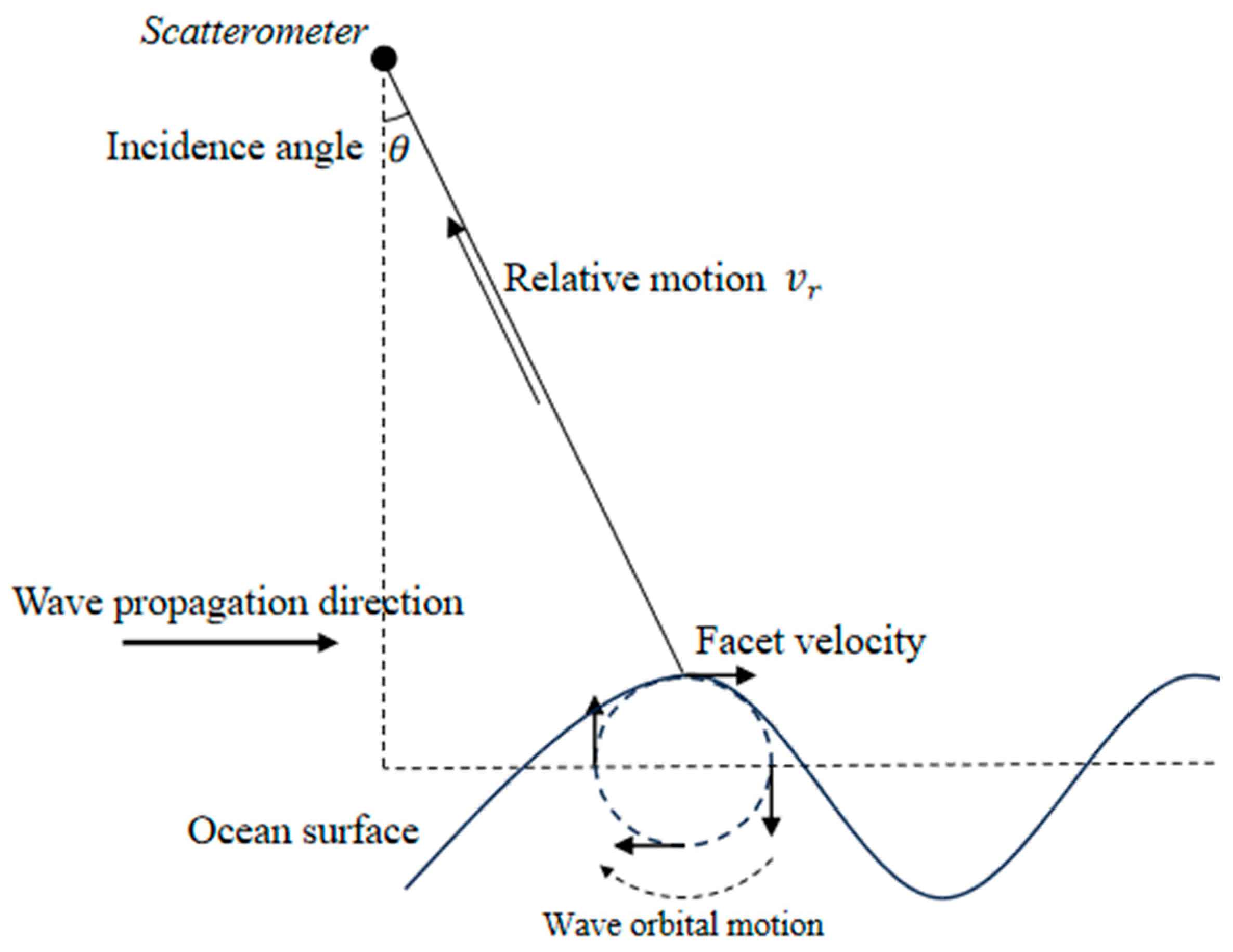
2.1. Measurement Principle

When there is a relative movement between the radar and observation target, the Doppler effect occurs, and the relationship between radial velocity of the moving target and Doppler frequency is [12]

$${\mathrm{f}}_{\mathrm{d}}=-\frac{2\mathrm{v}}{\mathsf{\lambda }}\mathrm{s}\mathrm{i}\mathrm{n}\mathsf{\theta }\mathrm{c}\mathrm{o}\mathrm{s}\mathsf{\phi }$$

(1)

where $v$ is the relative radial velocity between the moving target and radar, $\theta$ is the incidence angle, $\phi$ is the relative azimuth angle, and Doppler frequency is negative when the target is moving away from the radar and positive when the target approaches the radar. So, the Doppler of radar echoes backscattered is proportional to the line-of-sight velocity of the moving target. Figure 1 shows the diagram of the look geometry of the Doppler scatterometer to measure sea surface motion similar to Figure 6a in [11].

In the principle of interferometry, the radar echoes of successive pulses at short intervals are correlated, and the interferometric phase obtained can be used for direct frequency measurements. The two continuous echoed signals are given by

$$\begin{gathered} S_1=A_{1}exp\left[j\right(2\pi f_c{t}_i+{\phi }_1\left)\right] \\ {S}_2=A_{2}exp\left[j\right(2\pi f_c{t}_i+{\phi }_2\left)\right] \end{gathered}$$

(2)

Here, $A_1$ and $A_2$ are the amplitude determined by the radar equation

$$A_i=\sqrt{\frac{P_t{\lambda }^2{G}^2}{{\left(4\pi \right)}^3{R}_{Look}^4}\ast {\sigma }_0}$$

(3)

$P_t$, $\lambda$ and $G$ are instrument parameters, and $R_{look}$ is the distance from the scatter to the scatterometer. ${\sigma }_0$ is the target backscatter and is directly related to wind speeds and wind directions of the sea surface (here, the Ka-band of GPM data is used as a reference) [39,40]. $f_c$ is the carrier frequency of transmitted signals, $t_i$ is the time delay, and ${\phi }_1$ and ${\phi }_2$ are the echoed phases. The delay time of each scatter $t_i$ is given by

$$t_i=t-\frac{2R_{look}\left(i\right)}{c},$$

(4)

where i represents the sampling point in every signal footprint. Then, the phase difference is written as a

$$\Delta \phi ={\phi }_2-{\phi }_1=2\pi f_d\Delta \tau ,$$

(5)

where $\Delta \tau$ is the time interval. So, the Doppler frequency is embodied in the interferometric phase, and the relationship between the Doppler frequency and radial velocity (projected on the line of sight) of the sea surface is established based on Equations (1) and (5). The Doppler obtained by phase difference includes the satellite movement and the ocean surface motion. Then, the measured Doppler spectrum is considered as the distribution of Doppler frequencies associated with the moving ocean scatter after removing the Doppler resulting from satellite velocity. In Formula (5), we assume that the look geometry of antenna does not change and neglect the effect of the spatial translation and range resolution of the footprint.

In the return signal processing, the interfered form is expressed as [41]

$$\gamma =\frac{E\left\{S_1{S}_2^{*}\right\}}{\sqrt{E\left\{{\left|S_1\right|}^2\right\}E\left\{{\left|S_2\right|}^2\right\}}}$$

(6)

where E is the expectation operator. The interferometric phase is defined as

$${\varnothing }_{int}=arg\left(\gamma \right)$$

(7)

And then the radial velocity is

$$v_r=-\frac{{\varnothing }_{int}\lambda }{4\pi \Delta \tau }$$

(8)

In principle, the instrument obtains the total radial Doppler velocity due to the relative motion of the surface roughness, which includes all types of currents (sea-level-driven, wind-driven, density-driven and tides), and all types of waves (surface wind-waves, swell, and internal waves). The main contributions to the surface motion are expected to wind-induced drift (Ekman current + Stokes drift), wind-waves, geostrophic and non-geostrophic currents. Thompson has shown that the motion of long gravity waves shifts and broadens the peak of the Doppler spectrum [37]. Wind wave effects on Doppler measurement are needed to analyze.

The measured ocean surface motion includes the orbital velocity of the long waves, wind drift velocity, and ocean surface currents [42]. These contributions can be expressed as

$$U_r=U_C+U_{WV}+U_S$$

(9)

where $U_r$ is the total ocean velocity and $U_C$ is the motion (it is also sometimes called background current) independent of the local wind and waves. The Stokes drift $U_S$ due to the orbital motion of water is highly correlated with the local wind stress. $U_{WV}$ is the wind-wave-induced Doppler velocity, and the orbital velocity of the long gravity wave $U_{Orbital}$ plays a major role. Thus, this calculation requires a linear superposition model of sea surface and a suitable wave spectrum. Therefore, the parameters of DS depend on the parameters of large-scale waves, and the DC obtained from the first-order moment of the Doppler spectrum is closely related to the Doppler generated by the total motion of the sea surface. To accurately obtain the ocean surface current information, the contribution of the wind wave must be estimated.

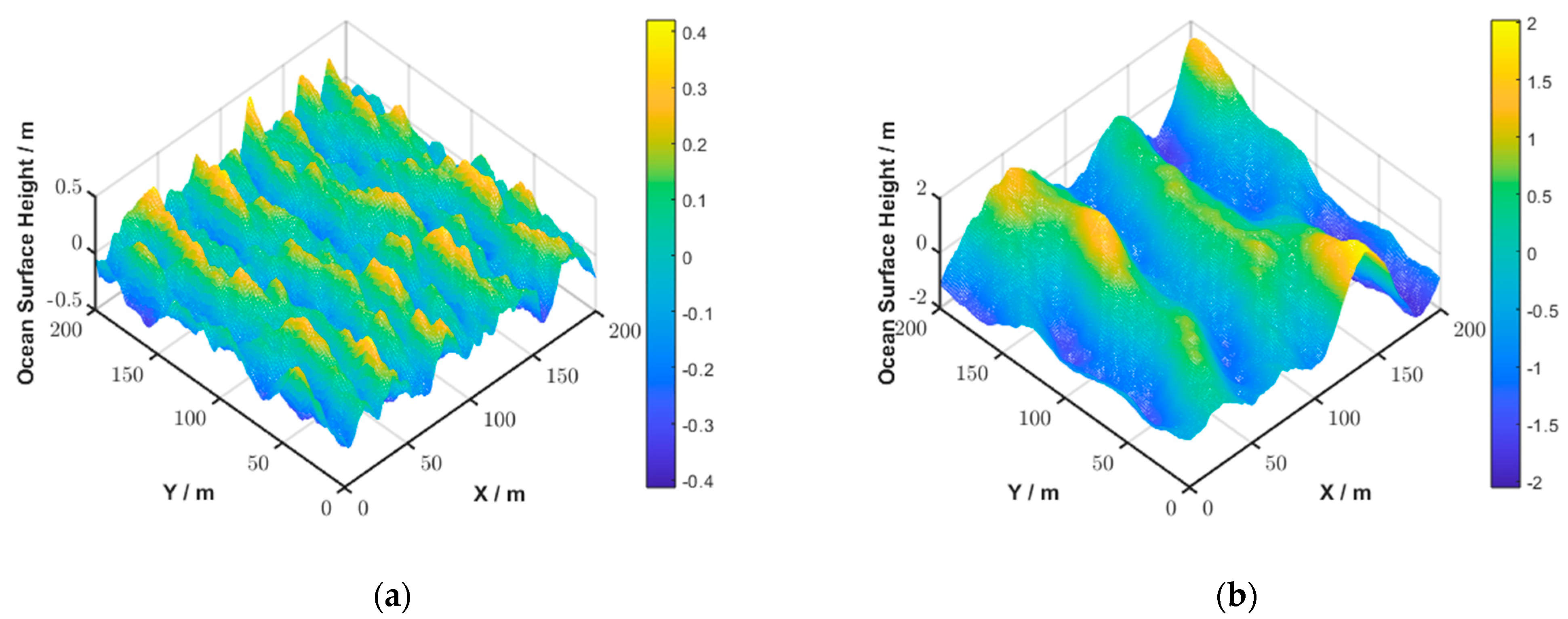
2.2. Dynamic Ocean Surface Generation

Fluctuation in the ocean surface is a complex random movement. For convenience of the study, an ocean surface can be considered as a superposition of many sine waves with different frequencies, amplitudes, phases, and propagation directions according to Fourier theory. When the ocean surface is fully developed, saturated and stable, it is generally considered that the ocean surface fluctuation during the detection cycle is a smooth random process. An ocean surface profile can be expressed as [43]

$$s\left(x,y,t\right)=\sum _{n=0}^N{A}_{n}sin[k_{nx}\left(x+v_{x}t\right)+k_{ny}\left(y+v_{y}t\right)-{\omega }_{n}t+{\phi }_n]$$

(10)

where $A_n$ is the amplitude of the ocean surface; $k_{nx}$ and $k_{ny}$ are the wavenumber components; $v_x$ and $v_y$ are the surface velocity in the x and y directions, respectively; ${\omega }_n$ is the angular frequency related to the acceleration of gravity and wavenumber; and ${\phi }_n$ is a random phase. The surface velocity contains the wave orbital velocity (dependent on the wavenumber) and background current in the $v_x$ and $v_y$. Generally, the sub-mesoscale current magnitude is small (usually less than 0.5 m/s). Meanwhile, we do not consider the wave–current interaction in the simulation.

The $A_n$ in (10) is given by

$$A_n(k,\phi )={\left[2\left(W_E\left(k,\phi \right)\Delta k\right)\right]}^{0.5}$$

(11)

where $W_E\left(k,\phi \right)$ is the 2-D directional wave number spectrum. In this work, we use the Elfouhaily spectrum to generate random ocean surfaces. It is widely used in radar probing of the ocean surface. The full wavenumber wave spectrum is expressed as the sum of low- and high-frequency regimes and Elfouhaily’s directional expression is as follows [36]:

$$S_E\left(k\right)=(B_l+B_h)/k^3,$$

(12)

$$W_E\left(k,\phi \right)=k^{-1}{S}_E\left(k\right)\Phi \left(k,\beta \right),$$

(13)

where $S_E\left(k\right)$ is the sum of two capillary and gravity components; $B_l\left(k\right)$ is the low-frequency part defined as Equation (31) in [44], and $B_h\left(k\right)$ is the high-frequency part defined as Equation (40) in [44]. $S_E\left(k\right)$ is the isotropic part of the spectrum, and $\Phi \left(k,\beta \right)$ is the angular function. $k$ and $\beta$ are the spatial wave number and the wind direction, respectively. We assume that the ocean moves towards the x-axis positive direction in the following simulation. Then, we can obtain the ocean surface height by the ocean surface model. Figure 2 represents a typical dynamic fully developed ocean surface about 200 m × 200 m with a 10 m/s wind speed at a time.

Within the framework of the linear superposition model, the ocean surface is represented as a superposition of different wave components, assuming that the heights of large-scale waves and ripples are not correlated. At small incidence angles (<10°), backscattering is quasi-specular, and the presence of large-scale wave components contributes to surface curvature. Large-scale waves affect the scatterers by varying the local incidence angle (tilt modulation) and changing the spectral density of the resonant ripple with the wave profile (hydrodynamic modulation) [45]. Using the ocean surface model, we can obtain the echoed signals of two moments, $S_1$ and $S_2$. Using Equations (5)–(7), we can calculate the total radial velocity $v_r$

$$v_r=U_{r}sin\theta +v_{p}sin\theta .$$

(14)

And the Doppler shift in Equation (1) is given by

$$f_d=-\frac{2v_r}{\lambda }=-\frac{2(U_r\mathrm{s}\mathrm{i}\mathrm{n}\theta +v_p\mathrm{s}\mathrm{i}\mathrm{n}\theta )}{\lambda }.$$

(15)

2.3. Simulations

To analyze the Doppler spectrum centroid induced by the ocean states in a spaceborne condition, information on the scatterometer incidence angle θ, radar electro-magnitude wavelength λ, and time interval τ, is necessary. Based on the previous study, the Ka-band is more sensitive to surface conditions [46], and we adopt the parameters as follows to investigate the variations in ocean current offset induced by wind waves.

In this work, the irradiated ocean surface is approximately 1.4 km × 1.4 km when the antenna beamwidth is 0.15°, and the surface grid sampling points are 1 m × 1 m. The wave number resolution dk = 2 pi/length ocean = 0.004 rad m⁻¹.

We can obtain the Doppler spectrum from the interferometric phase of the received signal. Before the Fourier transform, we removed the carried frequency by

$$S_D=S\cdot e^{-j2\pi f_{c}t}=\sum A_i\exp \left\{j2\pi f_d\left(i\right)t_i\right\},$$

(16)

where $A_i$ is determined by the radar equation and modulated by the backscattering coefficient. The expression of the Doppler spectrum $F_D$ is the Fourier transform of $S_D$:

$$F_D\left(f\right)={\int }_{-\infty }^{+\infty }{S}_D{e}^{-j2\pi ft}dt.$$

(17)

The sea state determines the measured Doppler shift and width. In [24], this idea was presented graphically. The Doppler spectrum shift $f_{sh0}$ is determined as follows [47]:

$$f_{sh0}=\frac{\int \omega S\left(\omega \right)d\omega }{\int S\left(\omega \right)d\omega }$$

(18)

and the broadening of the Doppler spectrum $\Delta f_{10}$ is

$$\Delta f_{10}=2\sqrt{(\frac{\int {\omega }^{2}S\left(\omega \right)d\omega }{\int S\left(\omega \right)d\omega }-{f_{sh0}}^2)}$$

(19)

assuming that the shape of the Doppler spectrum is Gaussian.

However, under spaceborne conditions, the satellite moves fast and illuminates several square kilometers per footprint. To accurately study the motion characteristics of the ocean surface, the influence of the platform Doppler must be removed, and the remaining Doppler velocity or Doppler shift is related to ocean surface dynamics. The platform velocity contribution is eliminated by

$$f_{sh}=f_{sh0}-\frac{2v_p\mathrm{s}\mathrm{i}\mathrm{n}\theta }{\lambda }$$

(20)

When the instrument antenna rotates around a vertical axis, the Doppler velocity sinusoidally changes due to positive or negative line of sight velocity and the azimuth direction of the antenna. The typical velocity of a spaceborne instrument is approximately 7000 m/s; then, the platform Doppler velocity is approximately ±732 m/s when the incidence angle is 6°, i.e., the platform Doppler frequency is 0.174 MHz.

Moreover, the presence of waves broadens the Doppler spectrum. And the antenna beamwidth greatly impacts the Doppler spectrum, especially broadening. Raney et al. [48] showed the Doppler broadening by the antenna beam (neglecting the Earth’s rotation effect):

$$\Delta f_{Dop}\approx \frac{2v_p}{\lambda }\mathrm{s}\mathrm{i}\mathrm{n}\mathsf{\Delta }\xi$$

(21)

where $\mathsf{\Delta }\xi$ is the antenna beamwidth. Therefore, for a rotating spaceborne Doppler measurement, the variation in the signal Doppler spectrum comes from the difference in the ocean surface velocity in the footprint and the beamwidth.

To understand this modulation on the Doppler spectrum, we analyze the effects of different ocean motion and the platform velocity as shown in Figure 3. We generate the dynamic ocean surface to obtain the Doppler spectrum with different broadening sources and set the Doppler measurement system parameters as presented in

Table 1. Platform parameters in this study.

Parameters	Value
Carrier Frequency	35.75 GHz
Carrier Wavelength	0.84 cm
Incidence Angle	6°
PRF	20 kHz
Antenna 3 dB beamwidth	0.15°
Satellite Orbital Height	520 km
Platform Velocity	7000 m/s

. We obtain the Doppler spectrum produced by ocean surface motion under the illumination of antenna beamwidth 0.15° at a 10 m/s wind speed, 0°azimuth angle with background current of 0.5 m/s when platform velocity is zero. We then set the platform velocity to 7000 m/s and obtain the Doppler spectrum considering ocean motion and platform velocity. Figure 3a shows the Doppler without platform velocity. Figure 3b shows the Doppler spectrum after theoretically adding the motion of platform. If the platform velocity is considered, the platform’s Doppler frequency generated must be added to the frequency shift over the Doppler spectrum. In fact, with the short-term interference under spaceborne conditions, the spectrum has been broadened within the antenna beamwidth. Figure 3c shows the Doppler spectrum considering the ocean motion and satellite platform velocity modulated. In the resulting Doppler spectrum of the signals, we can only subtract the Doppler shift caused by the known platform motion, and the rest of the spectrum is the focus of our analysis. Figure 3d shows the Doppler spectrum after removing the platform Doppler. Figure 3 shows that the platform velocity produces a widening that is more evident than ocean surface motion.

After removing the platform Doppler component, the residual Doppler shift or Doppler velocity anomaly is related to the kinematics of the ocean surface, which is of interest here. From the signal echo perspective, the Doppler spectrum varies with the look geometry and ocean states. In this section, we present simulation analysis for different cases of the ocean state, and the radial velocity of measurement accuracy is evaluated as follows:

$$\Delta v_r=-\pi \Delta f/k_e$$

(22)

3. Results

Aimed at observing the wind wave and current simultaneously, we describe the dynamic ocean as wind speeds. The simulation process is similar to the process described above in Figure 3. The figure below shows the spectrum with different ocean states and look geometry after removing platform velocity.

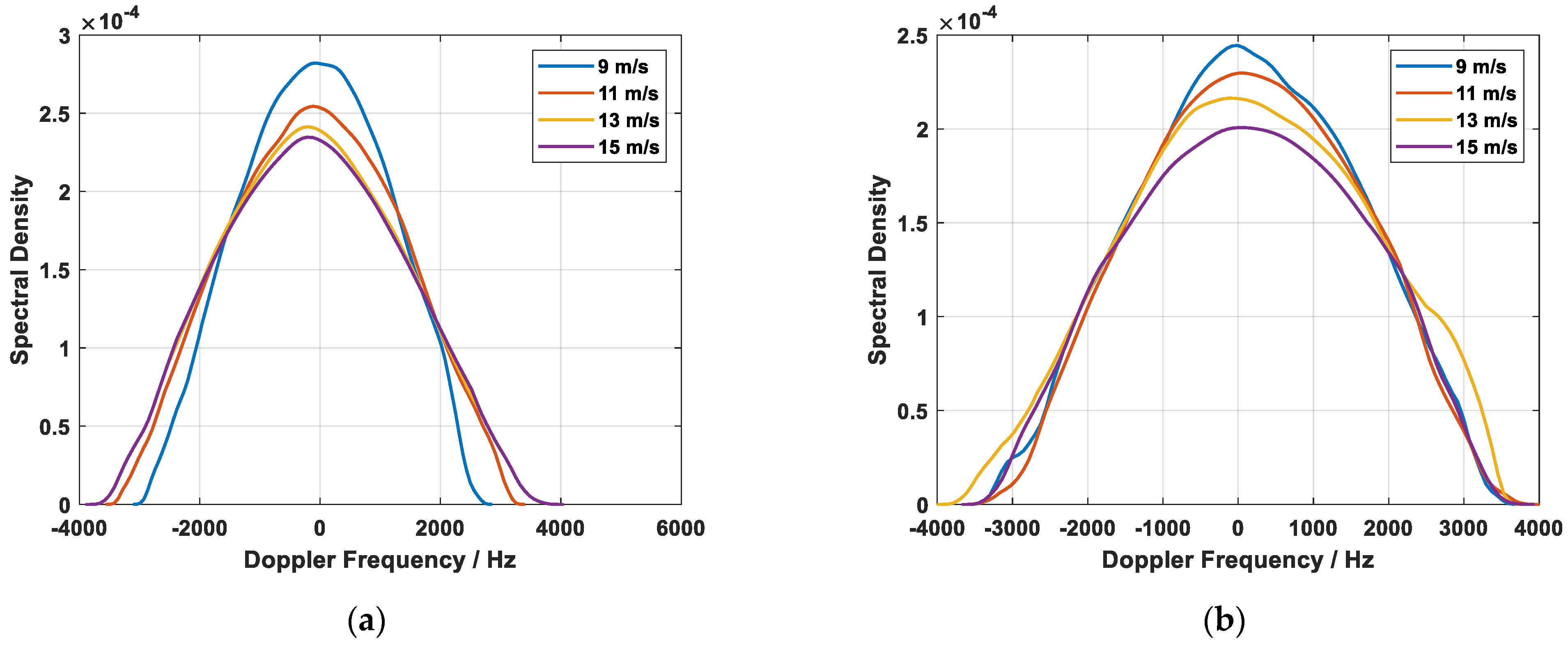
3.1. Doppler Spectrum Variation with Wind Speeds

The wind speed mainly affects the slope of the ocean surface, which is reflected in the Doppler shift and broadening. When the direction of satellite movement is consistent with the sea surface, and the antenna is along the track, that is, the observation azimuth angle is 180 degrees, the Doppler shift and the broadening increase with the increasing ocean surface height. When the look direction is perpendicular to the direction of the ocean movement, the Doppler centroid should be zero with some broadening. Figure 4 shows the Doppler spectra of the ocean itself without platform velocity. And

Table 2. Simulated Doppler parameters varying with wind speeds when at a 180-degree azimuth angle.

Ux	9 m/s	11 m/s	13 m/s	15 m/s
$f_{sh}$ $\Delta f_{10}$	44.4 609	46.4 721	52.4 813	57.4 1289

and

Table 3. Simulated Doppler parameters varying with wind speeds when at 90-degree azimuth angle.

Ux	9 m/s	11 m/s	13 m/s	15 m/s
$f_{sh}$ $\Delta f_{10}$	−1.3 553	−1.0 632	3.8 780	3.3 1226

show the specific values of the simulated Doppler parameters varying with wind speeds when at 180-and 90-degree azimuth angles, respectively.

Figure 5a shows the Doppler spectrum with the wind wave at a zero-degree azimuth angle after removing the platform Doppler as in Figure 3d. Likewise, Figure 5b shows the Doppler spectrum with a 90-degree azimuth angle.

Table 4. Simulated Doppler shift with wind speeds along the track.

Ux	7 m/s	9 m/s	11 m/s	13 m/s	15 m/s
$\mathrm{measured} f_{sh}$	−46.3	−57.5	−65.1	−70.7	−76.6
wind wave	−28	−32	−34	−40	−45
$f_{current}$	−12.4	−12.4	−12.4	−12.4	−12.4

shows the specific values of Doppler shift and broadening with the wind wave, and they are closely related to the antenna parameters, look geometries and ocean states. In Table 4, the simulated DC indicates the Doppler centroid calculated under the spaceborne condition after removing Doppler via platform motion, and the ‘true’ Doppler shift is determined based on the second-moment wave spectrum and antenna pattern [49].

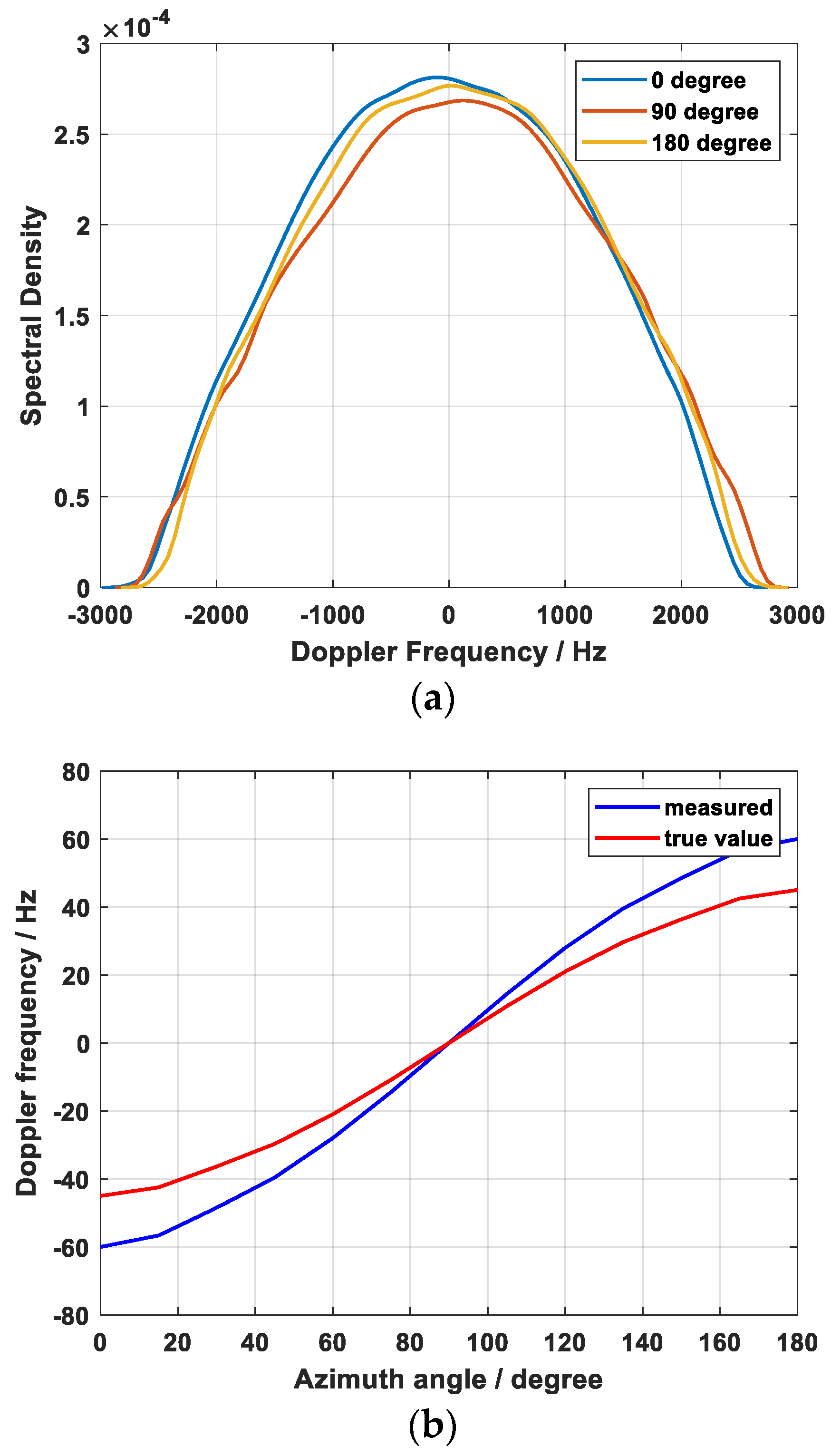
3.2. Doppler Spectrum Variation with Different Azimuth Angles

We assume that the ocean moves towards the x-axis positive direction in the following simulation. At the same time, the direction of the satellite movement is also positive on the x-axis. The azimuth angle in the figures is the angle between the antenna and the direction of motion. The simulated Doppler centroid is different from the ‘true’. Figure 6a shows the observed Doppler spectrum at different azimuth angles of 0, 90, and 180 degrees under a certain ocean state condition. Figure 6b shows the DC trend with different azimuth angles compared with the ‘true’ Doppler. According to Equation (22), the measured deviation is less than 0.1 m/s. The platform’s rapid movement and the short observation duration of the same area lead to fewer echo signal sampling points and lower frequency resolution, and there is a certain random error in the statistical estimation of the Doppler spectrum. By comparison, the measured deviations are considered acceptable.

4. Discussion

Doppler scatterometry can obtain surface backscattering coefficients to retrieve wind and wave information and can also obtain surface kinetic components to current. In this paper, a two-scale scattering model was adopted (without considering long-short wave interactions), and the measured Doppler spectrum of ocean surface was explicitly affected by wind waves. Based on the linear superposition model, backscattering at small incidence angles is quasi-specula and is sensitive to the long-wave inclination of the surface. The dependences of the backscattering coefficients on the wind speed and wave intensity have already been skillfully acquired. The microwave radar scatterometer generally measures processes at tens of kilometers, while sub-mesoscale oceanic dynamic features are not resolved. So, the Doppler spectrum contains more information about the ocean surface and is a more promising information parameter to retrieve information about ocean dynamics.

The Doppler spectrum shape and moments were analyzed. Simulations of the Doppler spectrum under different conditions could lead to relative differences in Doppler shifts. The different wind and wave motions were the dominant contribution to the Doppler spectrum in the studies. The current retrieval accuracy also depended on the accuracy of wind and wave vectors via wind-wave bias removal in actual measurements. This sensitivity varied with the look of geometries and ocean states, but we limited our assessment to the incidence angle and along the track for simplicity. The measurement deviation along the trace direction is at the maximum and is at its smallest in the cross-track. At moderate wind-wave conditions, the Doppler velocity offset can be less than 0.1 m/s, which is beneficial for detecting the open ocean surface motion.

Based on the background of the joint observation of wind, waves, and current, we focus on the contribution of wind and waves to the Doppler centroid in the simulation and do not consider the influence of breaking waves for the time being. Due to the limitations of linear superposition, adding nonlinear components to the dynamic model is difficult. The study of Yurovsky et al. based on actual measurements is very meaningful. It also analyzes the Doppler centroid in the composite scattering mechanism that exists at a 20-degree incidence angle [38]. The breaking wave that exists affects the asymmetry of backscattering, resulting in anomalies in the upwind and downwind of the Doppler centroid. However, the impact between the upwind and downwind is not particularly significant at small incidence angles, especially on instantaneous Doppler shift under spaceborne conditions. It provides a reliable benchmark for our future simulations. Certainly, we are supposed to pay more attention to the breaking waves, especially in high ocean states. As a larger fraction of the ocean is covered by whitecaps and waves are generally steeper, the linear wave theory for the surface velocities may require extensions to take into account the nonlinear kinematics of steep or breaking waves.

References

1. Chen, R.; Flierl, G.R.; Wunsch, C. A Description of Local and Nonlocal Eddy–Mean Flow Interaction in a Global Eddy-Permitting State Estimate. J. Phys. Oceanogr. 2014, 44, 2336–2352. [Google Scholar] [CrossRef]
2. Centurioni, L.R.; Turton, J.; Lumpkin, R.; Braasch, L.; Brassington, G.; Chao, Y.; Charpentier, E.; Chen, Z.; Corlett, G.; Dohan, K.; et al. Global in situ Observations of Essential Climate and Ocean Variables at the Air–Sea Interface. Front. Mar. Sci. 2019, 6, 419. [Google Scholar] [CrossRef]
3. Lumpkin, R.; Johnson, G.C. Global ocean surface velocities from drifters: Mean, variance, El Niño–Southern Oscillation response, and seasonal cycle. J. Geophys. Res. Oceans 2013, 118, 2992–3006. [Google Scholar] [CrossRef]
4. Wang, S.D.; Shen, Y.M.; Zheng, Y.H. Two-dimensional numerical simulation for transport and fate of oil spills in seas. Ocean Eng. 2005, 32, 1556–1571. [Google Scholar] [CrossRef]
5. Klemas, V. Tracking Oil Slicks and Predicting their Trajectories Using Remote Sensors and Models: Case Studies of the Sea Princess and Deepwater Horizon Oil Spills. J. Coast. Res. 2010, 26, 789–797. [Google Scholar] [CrossRef]
6. McIntosh, R.E.; Swift, C.T.; Raghavan, R.S.; Baldwin, A.W. Measurement of Ocean Surface Currents from Space with Multifrequency Microwave Radars—A System Analysis. IEEE Trans. Geosci. Remote Sens. 1985, GE-23, 2–12. [Google Scholar] [CrossRef]
7. Laws, K.E.; Vesecky, J.F.; Paduan, J.D. Error assessment of HF radar-based ocean current measurements: An error model based on sub-period measurement variance. In Proceedings of the 2011 IEEE/OES 10th Current, Waves and Turbulence Measurements (CWTM), Monterey, CA, USA, 20–23 March 2011; pp. 70–76. [Google Scholar]
8. Gould, J.; Sloyan, B.; Visbeck, M. Chapter 3—In Situ Ocean Observations: A Brief History, Present Status, and Future Directions. In International Geophysics; Siedler, G., Griffies, S.M., Gould, J., Church, J.A., Eds.; Academic Press: Cambridge, MA, USA, 2013; Volume 103, pp. 59–81. [Google Scholar]
9. Kudryavtsev, V.; Akimov, D.; Johannessen, J.; Chapron, B. On radar imaging of current features: 1. Model and comparison with observations. J. Geophys. Res. Oceans 2005, 110, C07016. [Google Scholar] [CrossRef]
10. Johannessen, J.A.; Kudryavtsev, V.; Akimov, D.; Eldevik, T.; Winther, N.; Chapron, B. On radar imaging of current features: 2. Mesoscale eddy and current front detection. J. Geophys. Res. Oceans 2005, 110, C07017. [Google Scholar] [CrossRef]
11. Chapron, B.; Collard, F.; Ardhuin, F. Direct measurements of ocean surface velocity from space: Interpretation and validation. J. Geophys. Res. Oceans 2005, 110, C07008. [Google Scholar] [CrossRef]
12. Romeiser, R.; Thompson, D.R. Numerical study on the along-track interferometric radar imaging mechanism of oceanic surface currents. IEEE Trans. Geosci. Remote Sens. 2000, 38, 446–458. [Google Scholar] [CrossRef]
13. Martin, A.C.H.; Gommenginger, C.; Marquez, J.; Doody, S.; Navarro, V.; Buck, C. Wind-wave-induced velocity in ATI SAR ocean surface currents: First experimental evidence from an airborne campaign. J. Geophys. Res. Oceans 2016, 121, 1640–1653. [Google Scholar] [CrossRef]
14. Martin, A.C.H.; Gommenginger, C. Towards wide-swath high-resolution mapping of total ocean surface current vectors from space: Airborne proof-of-concept and validation. Remote Sens. Environ. 2017, 197, 58–71. [Google Scholar] [CrossRef]
15. Martin, A.C.H.; Gommenginger, C.P.; Quilfen, Y. Simultaneous ocean surface current and wind vectors retrieval with squinted SAR interferometry: Geophysical inversion and performance assessment. Remote Sens. Environ. 2018, 216, 798–808. [Google Scholar] [CrossRef]
16. Trampuz, C.; Gebert, N.; Placidi, S.; Hendriks, I.; Speziali, F.; Navarro, V.; Martin, A.; Gommenginger, C.; Suess, M.; Meta, A. The Airborne Interferometric and Scatterometric radar instrument for Accurate Sea Current and Wind Retrievals. In Proceedings of the EUSAR 2018, 12th European Conference on Synthetic Aperture Radar, Aachen, Germany, 4–7 June 2018; pp. 1–6. [Google Scholar]
17. Martin, A.; Macedo, K.; Portabella, M.; Marié, L.; Marquez, J.; McCann, D.; Carrasco, R.; Duarte, R.; Meta, A.; Gommenginger, C.; et al. OSCAR: A new airborne instrument to image ocean-atmosphere dynamics at the sub-mesoscale: Instrument capabilities and the SEASTARex airborne campaign. In Proceedings of the EGU23, the 25th EGU General Assembly, Vienna, Austria, 23–28 April 2023; p. EGU-9940. [Google Scholar]
18. Le Traon, P.Y.; Morrow, R. Chapter 3 Ocean Currents and Eddies. In International Geophysics; Fu, L.-L., Cazenave, A., Eds.; Academic Press: Cambridge, MA, USA, 2001; Volume 69, pp. 171–215. [Google Scholar]
19. Du, Y.; Dong, X.; Jiang, X.; Zhang, Y.; Zhu, D.; Sun, Q.; Wang, Z.; Niu, X.; Chen, W.; Zhu, C.; et al. Ocean surface current multiscale observation mission (OSCOM): Simultaneous measurement of ocean surface current, vector wind, and temperature. Prog. Oceanogr. 2021, 193, 102531. [Google Scholar] [CrossRef]
20. Rodríguez, E.; Bourassa, M.A.; Chelton, D.; Farrar, J.T.; Long, D.G.; Perkovic-Martin, D.; Samelson, R. The Winds and Currents Mission Concept. Front. Mar. Sci. 2019, 6, 438. [Google Scholar] [CrossRef]
21. Rodríguez, E.; Wineteer, A.; Perkovic-Martin, D.; Gál, T.; Stiles, B.W.; Niamsuwan, N.; Monje, R.R. Estimating Ocean Vector Winds and Currents Using a Ka-Band Pencil-Beam Doppler Scatterometer. Remote Sens. 2018, 10, 576. [Google Scholar] [CrossRef]
22. Ardhuin, F.; Brandt, P.; Gaultier, L.; Donlon, C.; Battaglia, A.; Boy, F.; Casal, T.; Chapron, B.; Collard, F.; Cravatte, S.; et al. SKIM, a Candidate Satellite Mission Exploring Global Ocean Currents and Waves. Front. Mar. Sci. 2019, 6, 209. [Google Scholar] [CrossRef]
23. Nouguier, F.; Chapron, B.; Collard, F.; Mouche, A.A.; Rascle, N.; Ardhuin, F.; Wu, X. Sea Surface Kinematics from Near-Nadir Radar Measurements. IEEE Trans. Geosci. Remote Sens. 2018, 56, 6169–6179. [Google Scholar] [CrossRef]
24. Gommenginger, C.; Chapron, B.; Hogg, A.; Buckingham, C.; Fox-Kemper, B.; Eriksson, L.; Soulat, F.; Ubelmann, C.; Ocampo-Torres, F.; Nardelli, B.B.; et al. SEASTAR: A Mission to Study Ocean Submesoscale Dynamics and Small-Scale Atmosphere-Ocean Processes in Coastal, Shelf and Polar Seas. Front. Mar. Sci. 2019, 6, 457. [Google Scholar] [CrossRef]
25. López-Dekker, P.; Biggs, J.; Chapron, B.; Hooper, A.; Kääb, A.; Masina, S.; Mouginot, J.; Nardelli, B.B.; Pasquero, C.; Prats-Iraola, P.; et al. The Harmony Mission: End of Phase-0 Science Overview. In Proceedings of the 2021 IEEE International Geoscience and Remote Sensing Symposium IGARSS, Brussels, Belgium, 11–16 July 2021; pp. 7752–7755. [Google Scholar]
26. Chelton, D.; Schlax, M.G.; Freilich, M.H.; Milliff, R.F. Satellite Measurements Reveal Persistent Small-Scale Features in Ocean Winds. Science 2004, 303, 978–983. [Google Scholar] [CrossRef]
27. Fabry, P.; Recchia, A.; de Kloe, J.; Stoffelen, A.; Husson, R.; Collard, F.; Chapron, B.; Mouche, A.; Enjolras, V.; Johannessen, J.; et al. Feasibility Study of Sea Surface Currents Measurements with Doppler Scatterometers. In Proceedings of the ESA Living Planet Programme, 12th European Conference on Synthetic Aperture Radar, Edinburgh, UK, 9–13 September 2013. ESA Living Planet Programme. [Google Scholar]
28. Miao, Y.; Dong, X.; Bao, Q.; Zhu, D. Perspective of a Ku-Ka Dual-Frequency Scatterometer for Simultaneous Wide-Swath Ocean Surface Wind and Current Measurement. Remote Sens. 2018, 10, 1042. [Google Scholar] [CrossRef]
29. Torres, H.; Wineteer, A.; Klein, P.; Lee, T.; Wang, J.; Rodriguez, E.; Menemenlis, D.; Zhang, H. Anticipated Capabilities of the ODYSEA Wind and Current Mission Concept to Estimate Wind Work at the Air–Sea Interface. Remote Sens. 2023, 15, 3337. [Google Scholar] [CrossRef]
30. Fayne, J.V.; Smith, L.C.; Liao, T.H.; Pitcher, L.H.; Denbina, M.; Chen, A.C.; Simard, M.; Chen, C.W.; Williams, B.A. Characterizing Near-Nadir and Low Incidence Ka-Band SAR Backscatter from Wet Surfaces and Diverse Land Covers. IEEE J. Sel. Top. Appl. Earth Obs. Remote Sens. 2024, 17, 985–1006. [Google Scholar] [CrossRef]
31. Nouguier, F.; Chapron, B.; Collard, F.; Ardhuin, F. Synergy of Experimental, Theoretical and Numerical Approaches for a Better Understanding of Skim Near Nadir Ka-Band Doppler Measurements. In Proceedings of the IGARSS 2019—2019 IEEE International Geoscience and Remote Sensing Symposium, Yokohama, Japan, 28 July–2 August 2019; pp. 8027–8030. [Google Scholar]
32. Ardhuin, F.; Aksenov, Y.; Benetazzo, A.; Bertino, L.; Brandt, P.; Caubet, E.; Chapron, B.; Collard, F.; Cravatte, S.; Delouis, J.M.; et al. Measuring currents, ice drift, and waves from space: The Sea surface KInematics Multiscale monitoring (SKIM) concept. Ocean Sci. 2018, 14, 337–354. [Google Scholar] [CrossRef]
33. Elyouncha, A.; Eriksson, L.E.B.; Romeiser, R.; Ulander, L.M.H. Measurements of Sea Surface Currents in the Baltic Sea Region Using Spaceborne Along-Track InSAR. IEEE Trans. Geosci. Remote Sens. 2019, 57, 8584–8599. [Google Scholar] [CrossRef]
34. Wang, Y.; Zhang, Y.; He, M.; Zhao, C. Doppler Spectra of Microwave Scattering Fields from Nonlinear Oceanic Surface at Moderate- and Low-Grazing Angles. IEEE Trans. Geosci. Remote Sens. 2012, 50, 1104–1116. [Google Scholar] [CrossRef]
35. Hansen, M.W.; Kudryavtsev, V.; Chapron, B.; Johannessen, J.A.; Collard, F.; Dagestad, K.F.; Mouche, A.A. Simulation of radar backscatter and Doppler shifts of wave–current interaction in the presence of strong tidal current. Remote Sens. Environ. 2012, 120, 113–122. [Google Scholar] [CrossRef]
36. Ryabkova, M.; Karaev, V.; Guo, J.; Titchenko, Y. A Review of Wave Spectrum Models as Applied to the Problem of Radar Probing of the Sea Surface. J. Geophys. Res. Ocean. 2019, 124, 7104–7134. [Google Scholar] [CrossRef]
37. Yurovsky, Y.Y.; Kudryavtsev, V.N.; Chapron, B.; Grodsky, S.A. Modulation of Ka-Band Doppler Radar Signals Backscattered from the Sea Surface. IEEE Trans. Geosci. Remote Sens. 2018, 56, 2931–2948. [Google Scholar] [CrossRef]
38. Yurovsky, Y.Y.; Kudryavtsev, V.N.; Grodsky, S.A.; Chapron, B.J. Sea Surface Ka-Band Doppler Measurements: Analysis and Model Development. Remote Sens. 2019, 11, 839. [Google Scholar] [CrossRef]
39. Chu, X.; He, Y.; Karaev, V.Y. Relationships Between Ku-Band Radar Backscatter and Integrated Wind and Wave Parameters at Low Incidence Angles. IEEE Trans. Geosci. Remote Sens. 2012, 50, 4599–4609. [Google Scholar] [CrossRef]
40. Hossan, A.; Jones, W.L. Ku- and Ka-Band Ocean Surface Radar Backscatter Model Functions at Low-Incidence Angles Using Full-Swath GPM DPR Data. Remote Sens. 2021, 13, 1569. [Google Scholar] [CrossRef]
41. Abeysekera, S.S. Performance of pulse-pair method of Doppler estimation. IEEE Trans. Aerosp. Electron. Syst. 1998, 34, 520–531. [Google Scholar] [CrossRef]
42. Miao, Y.; Dong, X.; Bourassa, M.A.; Zhu, D. Effects of Different Wave Spectra on Wind-Wave Induced Doppler Shift Estimates. In Proceedings of the IGARSS 2020—2020 IEEE International Geoscience and Remote Sensing Symposium, Waikoloa, HI, USA, 26 September–2 October 2020; pp. 5705–5708. [Google Scholar]
43. Thompson, D.R. Calculation of Microwave Doppler Spectra from the Ocean Surface with a Time-Dependent Composite Model. In Radar Scattering from Modulated Wind Waves: Proceedings of the Workshop on Modulation of Short Wind Waves in the Gravity-Capillary Range by Non-Uniform Currents, Bergen aan Zee, The Netherlands, 24–26 May 1988; Komen, G.J., Oost, W.A., Eds.; Springer: Dordrecht, The Netherlands, 1989; pp. 27–40. [Google Scholar]
44. Elfouhaily, T.; Chapron, B.; Katsaros, K.; Vandemark, D. A unified directional spectrum for long and short wind-driven waves. J. Geophys. Res. 1997, 102, 15781–15796. [Google Scholar] [CrossRef]
45. Thompson, D.R.; Gotwols, B.L.; Keller, W.C. A comparison of Ku -band Doppler measurements at 20° incidence with predictions from a time-dependent scattering model. J. Geophys. Res. 1991, 96, 4947–4955. [Google Scholar] [CrossRef]
46. Yan, Q.; Zhang, J.; Fan, C.; Meng, J. Analysis of Ku- and Ka-Band Sea Surface Backscattering Characteristics at Low-Incidence Angles Based on the GPM Dual-Frequency Precipitation Radar Measurements. Remote Sens. 2019, 11, 754. [Google Scholar] [CrossRef]
47. Barrick, D. First-order theory and analysis of MF/HF/VHF scatter from the sea. IEEE Trans. Antennas Propag. 1972, 20, 2–10. [Google Scholar] [CrossRef]
48. Raney, R.K. Doppler properties of radars in circular orbits. Int. J. Remote Sens. 1986, 7, 1153–1162. [Google Scholar] [CrossRef]
49. Panfilova, M.; Ryabkova, M.; Karaev, V.; Skiba, E. Retrieval of the Statistical Characteristics of Wind Waves from the Width and Shift of the Doppler Spectrum of the Backscattered Microwave Signal at Low Incidence Angles. IEEE Trans. Geosci. Remote Sens. 2020, 58, 2225–2231. [Google Scholar] [CrossRef]
Figure 1. Schematic diagram of the look geometry of the Doppler scatterometer to measure the sea surface motion. The arrows represent the motion direction, and the curve represents the ocean surface.
Remotesensing 16 02083 g001
Figure 2. A typical dynamic ocean surface with (a) 6 m/s and (b) 10 m/s wind speed along the x-axis at a time.
Remotesensing 16 02083 g002
Figure 3. The Doppler spectrum of the along-track direction, 10 m/s wind speed: (a) ocean surface motion when platform velocity is zero; (b) ocean surface motion after theoretically adding the motion of the platform; (c) ocean motion and platform velocity modulated; (d) after removing the platform Doppler.
Remotesensing 16 02083 g003
Figure 4. Change in Doppler spectra with wind speeds without platform velocity when (a) at 180-degree azimuth angles and (b) at 90-degree azimuth angles.
Remotesensing 16 02083 g004
Figure 5. Change in Doppler spectrum with wind speeds when (a) at 0-degree azimuth angle and (b) 90-degree azimuth angle.
Remotesensing 16 02083 g005
Figure 6. (a) Doppler spectrum with a 10 m/s wind speed with 0-/90-/180-degree azimuth angles and (b) its DC with azimuth angles between 0 and 180° compared with the ‘true’ Doppler.
Remotesensing 16 02083 g006