Article

Characterizing Canopy Structure Variability in Amazonian Secondary Successions with Full-Waveform Airborne LiDAR

by
Aline D. Jacon
1,
Lênio Soares Galvão
1,
Rorai Pereira Martins-Neto
2,
Pablo Crespo-Peremarch
3,4,
Luiz E. O. C. Aragão
1,
Jean P. Ometto
5,
Liana O. Anderson
6,
Laura Barbosa Vedovato
7,
Celso H. L. Silva-Junior
8,
Aline Pontes Lopes
1,
Vinícius Peripato
1,
Mauro Assis
1,
Francisca R. S. Pereira
1,
Isadora Haddad
1,
Catherine Torres de Almeida
9,
Henrique L. G. Cassol
1,10 and
Ricardo Dalagnol
11,12,*
1
Earth Observation and Geoinformatics Division, National Institute for Space Research (INPE), São José dos Campos 12227-010, SP, Brazil
2
Faculty of Forestry and Wood Sciences, Czech University of Life Sciences Prague (CULS), Kamýcká 129, 165 00 Prague, Czech Republic
3
Geo-Environmental Cartography and Remote Sensing Group (CGAT), Department of Cartographic Engineering, Geodesy and Photogrammetry, Universitat Politècnica de València, Camí de Vera s/n, 46022 València, Spain
4
Escuela Superior de Ingeniería, Ciencia y Tecnología, Valencian International University—VIU, Calle Pintor Sorolla 21, 46002 València, Spain
5
General Coordination of Earth Science, National Institute for Space Research (INPE), São José dos Campos 12227-010, SP, Brazil
6
National Center for Monitoring and Early Warning of Natural Disasters (CEMADEN), São José dos Campos 12247-016, SP, Brazil
7
Institute for Technological Research (IPT), Av. Prof. Almeida Prado, Butantã, São Paulo 05508-901, SP, Brazil
8
Instituto de Pesquisa Ambiental da Amazônia (IPAM), SCN 211, Bloco B, Sala 201, Brasília 70836-520, GO, Brazil
9
Faculty of Agricultural Sciences of Vale do Ribeira-Câmpus de Registro, São Paulo State University (UNESP) Júlio de Mesquita Filho, Registro 11900-000, SP, Brazil
10
Bluebell Index, R. do Rocio, 291-Vila Olímpia, São Paulo 04552-000, SP, Brazil
11
Center for Tropical Research, Institute of the Environment and Sustainability, University of California, Los Angeles, CA 90095, USA
12
NASA-Jet Propulsion Laboratory, California Institute of Technology, Pasadena, CA 91109, USA
*
Author to whom correspondence should be addressed.
Remote Sens. 2024, 16(12), 2085; https://doi.org/10.3390/rs16122085
Submission received: 6 May 2024 / Revised: 30 May 2024 / Accepted: 6 June 2024 / Published: 9 June 2024
(This article belongs to the Special Issue Retrieving Leaf Area Index Using Remote Sensing)

Abstract

:
Full-waveform LiDAR (FWF) offers a promising advantage over other technologies to represent the vertical canopy structure of secondary successions in the Amazon region, as the waveform encapsulates the properties of all elements intercepting the emitted beam. In this study, we investigated modifications in the vertical structure of the Amazonian secondary successions across the vegetation gradient from early to advanced stages of vegetation regrowth. The analysis was performed over two distinct climatic regions (Drier and Wetter), designated using the Maximum Cumulative Water Deficit (MCWD). The study area was covered by 309 sample plots distributed along 25 LiDAR transects. The plots were grouped into three successional stages (early—SS1; intermediate—SS2; advanced—SS3). Mature Forest (MF) was used as a reference of comparison. A total of 14 FWF LiDAR metrics from four categories of analysis (Height, Peaks, Understory and Gaussian Decomposition) were extracted using the Waveform LiDAR for Forestry eXtraction (WoLFeX) software (v1.1.1). In addition to examining the variation in these metrics across different successional stages, we calculated their Relative Recovery (RR) with vegetation regrowth, and evaluated their ability to discriminate successional stages using Random Forest (RF). The results showed significant differences in FWF metrics across the successional stages, and within and between sample plots and regions. The Drier region generally exhibited more pronounced differences between successional stages and lower FWF metric values compared to the Wetter region, mainly in the category of height, peaks, and Gaussian decomposition. Furthermore, the Drier region displayed a lower relative recovery of metrics in the early years of succession, compared to the areas of MF, eventually reaching rates akin to those of the Wetter region as succession progressed. Canopy height metrics such as Waveform distance (WD), and Gaussian Decomposition metrics such as Bottom of canopy (BC), Bottom of canopy distance (BCD) and Canopy distance (CD), related to the height of the lower forest stratum, were the most important attributes in discriminating successional stages in both analyzed regions. However, the Drier region exhibited superior discrimination between successional stages, achieving a weighted F1-score of 0.80 compared to 0.73 in the Wetter region. When comparing the metrics from SS in different stages to MF, our findings underscore that secondary forests achieve substantial relative recovery of FWF metrics within the initial 10 years after land abandonment. Regions with potentially slower relative recovery (e.g., Drier regions) may require longer-term planning to ensure success in providing full potential ecosystem services in the Amazon.

Graphical Abstract

1. Introduction

Secondary successions are increasingly important components of landscapes modified by humans [1]. They consist of vegetation that grows naturally and transforms into secondary forests after the complete (or close to complete) removal of existing forest cover for anthropogenic use, agriculture, or pasture [2]. These regenerating secondary forests comprise up to a third of the Neotropical Forest area [3]. In Brazil, a total of 262,791 km2 of secondary forests, in the process of regeneration between 1986 and 2018, were mapped throughout the country, with the largest proportion (56%) identified in the Amazon biome [4].
The regeneration of secondary forests is essential in providing habitat for biodiversity and sustainable livelihoods for people [5,6], having great potential to mitigate climate change, among other ecosystem services [3]. These forests actively store carbon in aboveground biomass, partially offsetting carbon emissions from deforestation, forest degradation, fossil fuel burning, and other anthropogenic sources [3,7,8]. According to a study for the Neotropics region, secondary forests are highly productive, with an average net carbon uptake rate of 3.05 Mg·C·ha−1·year−1, after 20 years. This is equivalent to 11 times the rates of mature forests [7]. However, in the Brazilian Amazon, these carbon sequestration rates vary and are approximately 60% higher in the west (3.0 ± 1.0 Mg·C·ha−1·year−1) than in the east (1.3 ± 0.3 Mg·C·ha−1·year−1) due to several factors such as the difference in precipitation patterns or water deficit between both regions [8]. Thus, the difference in precipitation across regions is an important factor in the vegetation regeneration process. Comprehending the dynamics of vegetation growth with precipitation patterns is crucial for mitigating carbon and biodiversity loss resulting from potential disturbances, while also advocating for the adoption of public policies aimed at safeguarding secondary forests [4,8]. Other important factors that may be coupled together with the influence of precipitation on vegetation regrowth can include differences in soil composition and related fertility, radiation, land-use history, fire occurrence, and forest fragmentation [9,10,11].
As forest regeneration is influenced by processes operating at different spatial and temporal scales, remote sensing data can be used to study secondary successions in various ways. In the remote-sensing literature, discriminating stages of secondary succession remains challenging when using passive optical data [12], particularly when compared to airborne Light Detection and Ranging (LiDAR) data [13,14]. This challenge arises from the inherent difficulties in accurately measuring the vertical canopy structure using satellite images from Landsat instruments. As secondary succession progresses, notable changes in canopy structure typically occur, involving modifications in biophysical characteristics such as canopy height, leaf density, and understory vegetation. Given that vegetation regrowth is influenced by precipitation, it is important to understand the magnitude of such modifications in regions of the Amazon experiencing different water stress conditions. Thus, by fixing the precipitation in the experimental design, the analysis of LiDAR data obtained in distinct regions of the Amazon can contribute to improving this knowledge.
Due to the high heterogeneity and complexity of both primary and secondary forests, airborne LiDAR technology enables more accurate quantification of important structural attributes such as canopy height, leaf area density, basal area, and aboveground biomass [15,16,17,18,19,20]. In the scope of LiDAR technology, a type of data that has been little explored as a potential source of information is the Full Waveform (FWF). Some studies report the high potential of FWF airborne LiDAR metrics in describing and predicting structural parameters over forests with dense canopies and multiple strata [21,22,23,24,25,26]. However, as far as we know, there are no investigations in the literature addressing the use of this type of data, acquired by small-footprint aerial surveys, to characterize secondary forests of different successional stages in the Brazilian Amazon. The FWF technology captures backscattered energy by objects (e.g., canopy and ground) as a near-continuous signal at regular time intervals (approximately 1 ns) in a full-waveform indexed bin [27]. The signal is depicted as a waveform, with its associated amplitude values varying depending on the physical properties of the intercepted objects. Hence, FWF LiDAR records and stores significantly more information than the discrete-return LiDAR. Compared to discrete airborne LiDAR data, FWF data potentially have the advantage of improving the representation of forest structure, as the waveform contains the properties of all elements that intercept the path of the emitted beam [27]. With more information from different vertical layers, there is a greater chance of representing understory vegetation in forests with multiple strata [23].
In contrast, the use of FWF requires more elaborate procedures for data processing, a reason that may have hindered the widespread use of this type of data. This problem has been recently overcome with the development of new algorithms dedicated to FWF data analysis. An example is the Waveform LiDAR for Forestry eXtraction (WoLFeX) (v1.1.1), a software developed to process FWF airborne LiDAR data [28]. It allows for clipping, radiometric calibration, and extraction of metrics based on voxelization from FWF airborne LiDAR data. This software allows the calculation of several categories of metrics such as those related to vegetation height, peaks, understory information, and Gaussian decomposition.
In the Brazilian Amazon region, FWF airborne LiDAR data have been acquired over distinct sites of secondary successions in regions with different climatic conditions in terms of water deficit. This type of data has not been explored to inspect for eventual differences between climatic regions and successional stages as well as to understand the behavior of the different metrics with vegetation regrowth over time. Using machine learning techniques, we can identify the most appropriate FWF metrics for discriminating stages of secondary successions and those with more sensitivity to vegetation regrowth. All these possibilities require further studies.
In this context, we investigate for the first time the dynamics of changes in canopy structure and vegetation recovery along the vegetation gradient from early to advanced secondary successions with FWF airborne LiDAR data acquired in two Amazonian regions with distinct climatic conditions. Performing these analyses, we aim to address the following scientific questions: (i) Are there variations in FWF airborne LiDAR metrics (height, peaks, understory, and Gaussian decomposition) among successional stages within the same region and across regions? (ii) Does the relative vegetation recovery rate differ between regions for a given secondary succession and LiDAR metric? And (iii) does the classification of successional stages with Random Forest (RF) perform equally well and utilize the same FWF metrics when analyzed in climatically distinct scenarios?

2. Materials and Methods

2.1. Site Selection and Age Assignment of Secondary Successions

The study was conducted in the Brazilian Amazon Forest, where 309 circular sample plots, each one with a diameter of 50 m, were extracted from 25 airborne LiDAR transects. These transects were allocated in two regions characterized by distinct climatic regimes and referred to here as Wetter and Drier regions (Figure 1 and Figure S1—Supplementary Materials). The classification of these regions was based on the Maximum Cumulative Water Deficit—MCWD (mean MCWD value for the period 1986–2018) (Figure 1A), a climatic factor of high influence on vegetation regrowth [8]. The first region (Wetter), located in the south-central portions of the Amazon, presents a low mean MCWD (>−244.84 mm·yr−1), while the second region (Drier) in eastern Amazon shows a moderate to high mean MCWD (<=−244.84 mm·yr−1) (Figure 1B). This threshold represents the MCWD median value. It was selected to ensure minimum representation of sample plots at the different stages of secondary succession between the regions. The average annual precipitation range is approximately 2030 to 2730 mm and 1380 to 2060 mm for the Wetter and Drier regions, respectively.
In the current work, we assumed three stages of secondary succession: early (1 to 10 years—SS1), intermediate (11 to 20 years—SS2), and advanced (21 to 33 years—SS3) vegetation regrowth. The schematic representation of their differences in vegetation structure is shown in Supplementary Figure S2. The average age for SS1 was the same for both regions (6 years), and slightly differed in SS2 (Drier = 15 years and Wetter = 14 years), and SS3 (Drier = 30 years and Wetter = 27 years). The clustering into three stages was based on the availability of samples by age and region, following widely used approaches in secondary succession studies of tropical forests [12,14,26,29,30].
To assign the age of vegetation regrowth to each sample plot, we used the product generated in the study by Silva Junior et al. [4]. Based on the land cover maps from MapBiomas (Collection 6) [31] for the period from 1985 to 2018, they produced a map (using Landsat series images with 30-m spatial resolution) showing the age of secondary successions in Brazil ranging from 1 to 33 years. To reduce uncertainties in the data analysis, we conducted a quality assessment by tracking and confirming whenever possible the temporal trajectory of each land cover in Landsat images. Mature Forest (MF) was also considered as a reference of comparison and MapBiomas data were also used to identify MF areas, that is, stable forests from 1985 to 2018 in the LiDAR transects. Two other datasets were used to filter MF areas with low biomass (ESA-CCI AGB) [32] and with any sign of degradation (JRC-TMF) [33].
To reduce the influence of edges in the sample plots, a negative buffer of 60 m was applied around forest areas, and only areas larger than 1 hectare were included in the analysis [34]. A minimum distance of 300 m between the circular plots was established to avoid autocorrelation or spatial dependence of the FWF data. This value was determined from semivariogram analysis (Supplementary Figure S3). As shown in Figure 1C, the number of sample plots ranged from a minimum value of 7 (SS2) to a maximum value of 66 (Mature Forest—MF), both in the Wetter region.

2.2. Full-Waveform (FWF) Airborne LiDAR Data Acquisition and Derived Metrics

The 25 LiDAR transects used here are part of the Improving Biomass Estimation Methods for Amazon (EBA) project [19]. Full-waveform LiDAR data were acquired by the Trimble HARRIER 68i sensor onboard an airplane, covering transects in the ground with approximately 600 hectares (12 km × 0.5 km). The sensor operates in the near-infrared wavelength, producing a small footprint of 30 cm. The average flying height was 600 m above ground level with a maximum scanning angle of ±22.5 degrees off-nadir. The average pulse density was 4.8 pulses·m−2.
The processing and extraction of FWF metrics were carried out using WoLFeX software (v1.1.1) [28]. The required inputs for this software are files containing point data (.las file) and full-waveform data (.wdp file), respectively. Initially, each LiDAR data strip was clipped to the boundaries of the plots, followed by noise removal. Most FW LiDAR systems continue recording signals after the last return, allowing system noise determination. Therefore, samples with an intensity lower than a defined threshold are considered noise and discarded [35]. According to Martins-Neto [25], low-altitude flights over dense tropical forests may contain more noise. For this reason, after analyzing empirically some waveforms in different plots, we used a threshold for filtering and excluded from the analysis all waveforms with amplitudes below 5. A Gaussian filter was applied to remove the remaining noisy signals from the waveforms [28,36].
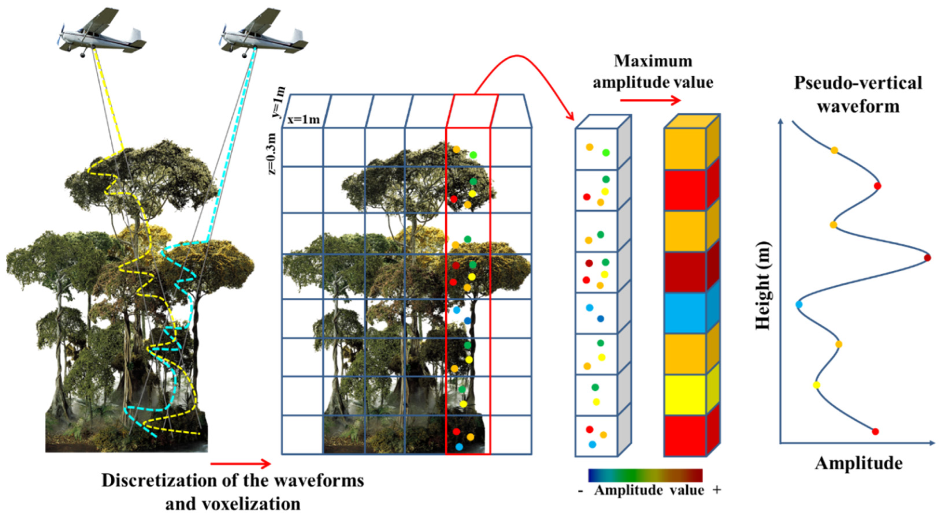
The next step involved voxelization of the data to generate pseudo-vertical waveforms. This procedure, proposed by Hermosilla et al. [36], is essential for data reduction and for handling the pulses emitted at off-nadir angles. This standardizes the acquisition of FWF metrics by generating new waveforms based on statistical amplitude values of each voxel (maximum, mean, or median) along a column from the canopy top to the ground. For this study, a voxel size of 1 × 1 × 0.3 m (dimensions in x, y, z) and maximum amplitude were used to generate pseudo-vertical waveforms (Figure 2).
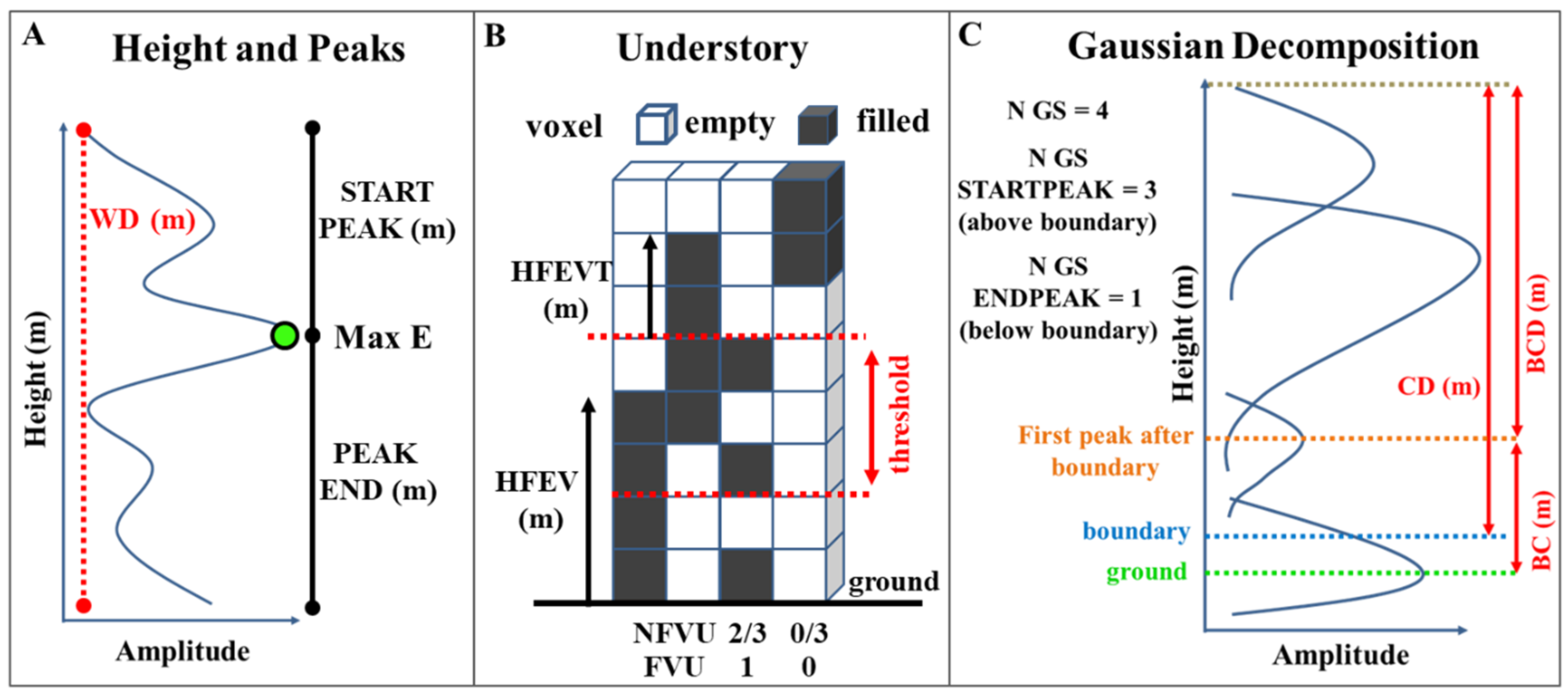
A total of 14 metrics were extracted within four categories related to height, peaks, understory, and Gaussian decomposition [28,37,38]. The metrics are described in Table 1 and graphically represented in Figure 3. Further detailed description can be found in Crespo-Peremarch and Ruiz [28]. For the understory metrics, a minimum threshold of 1 m and a maximum of 5 m were used to represent possible divisions between understory and canopy. As trajectory data were not provided, it was not possible to perform radiometric correction of the waveforms. Therefore, the selected metrics are not dependent on or are minimally influenced by the amplitude values (intensity). A digital terrain model (DTM) was generated for height normalization [39].

2.3. Data Analysis

We first explored how the FWF metrics varied across the gradient of successional stages and up to maturity using descriptive statistics, Pearson’s correlation coefficients, correlograms, and scatterplots. This analysis is important to understand the relationships between FWF metrics from the different categories (Table 1), considering the different successional stages (SS1, SS2, and SS3) and the MF.
To address the first scientific question and evaluate the differences in FWF metrics among successional stages and mature forest (SS1, SS2, SS3, and MF) within each region (Drier and Wetter) and between regions, we used the non-parametric Kruskal–Wallis and Mann–Whitney U tests. These tests are suitable for analyzing non-normally distributed data. Using this approach, we first fixed the region and tested for statistical differences between SS1, SS2, SS3, and MF. Then, we fixed the successional stage (SS1, SS2, or SS3) and tested for statistical differences in FWF metrics between the two climatically distinct regions.
Regarding the second scientific question, we calculated the Relative Recovery (RR) of FWF metrics following the methodology proposed by Poorter et al. [1]. This strategy ensures fair comparison between regions. The RR can be described as the percentage of metric recovery, calculated for each successional stage, compared to the mean values of the same metric calculated for mature forest, under the same growth conditions and without signs of recent human disturbances. Given that the metric values in the successional stages (SS) may be smaller or larger than the values for MF, we could not calculate recovery as M SSx/M MF, where M SSx is the metric value in the specific SS and M MF is the metric value for MF. We then calculated the divergence between the SS values and the MF values as ln (M SSx/M MF). To deal with positive and negative numbers, we took the negative exponential of the absolute value of the divergence: e−|ln (MSSx/MMF)|. This recovery ratio was multiplied by 100, ranging from close to zero (no recovery) to 100 (full recovery). The difference in RR of the FWF metrics between regions was evaluated for each successional stage using the non-parametric Mann–Whitney U test. All statistical analyses were performed in R environment version 4.2.2 [40].
The final stage of data analysis evaluated the discrimination of successional stages (SS1, SS2, and SS3) and MF using FWF LiDAR metrics. Instead of focusing solely on discrimination, the primary goal of this final stage of analysis was to assess the consistency of metric performance in distinguishing successional stages across both Drier and Wetter regions. To achieve this objective, we employed the widely recognized machine learning algorithm, Random Forest (RF). RF stands out among other classifiers due to its ability to generate highly accurate and stable predictions by leveraging multiple decision trees, thus mitigating the risk of overfitting [16,17,40,41,42]. For our analysis, another notable advantage of RF is its efficiency in selecting the most important variables during the discrimination process. In our current investigation, this attribute is particularly pertinent for assessing the predictive stability of LiDAR attributes in distinguishing successional stages across both climatic regions (Drier and Wetter). Therefore, to address the last scientific question, we examined the consistency of RF classification results in both regions and assessed the performance of FWF metrics for discrimination purposes. The basic idea is to identify the best set of FWF metrics to differentiate between the successional stages, while verifying the repeatability of the results in both regions. The RF classifier was applied separately to data from the Drier (164 sample plots) and the Wetter (145 sample plots) regions. For validating the results, a cross-validation approach using 5-fold with 10 times repetition was performed [17]. Different combinations of the RF parameters (number of trees—“Ntree”, and number of variables randomly sampled as candidates at each split—“mtry”) were tested in RF classification for each region. The best selected parameters were the ones that produced the highest overall classification accuracy.
To evaluate classification performance, we calculated the Precision, Recall, F1-score per class, overall or weighted F1-score by the number of samples of each class, and Overall Accuracy (OA). The precision quantifies the number of true positive predictions relative to the total number of positive predictions, while Recall quantifies the number of true positive predictions relative to the total number of actual positive instances in the dataset. Finally, the F1-score combines Precision and Recall through a harmonic mean into a single performance measure for a given class [41]. Although OA is not recommended for models where the number of classes is imbalanced, this measure is widely used in the literature and can be valid for comparison with other studies.
The RF classification was conducted in R [40] using the caret package [42]. We also evaluated the performance of FWF metrics on each region by ranking the importance of each metric for the overall accuracy of the RF classification. This result was provided by the varImp function in the caret package in R [42]. For each tree, the prediction accuracy on the out-of-bag portion of the data is recorded. Then the same procedure is repeated after permuting each predictor variable. The difference between the two accuracies is then averaged over all trees and normalized by the standard error.

3. Results

3.1. Variations in FWF Metrics within and across Circular Sample Plots

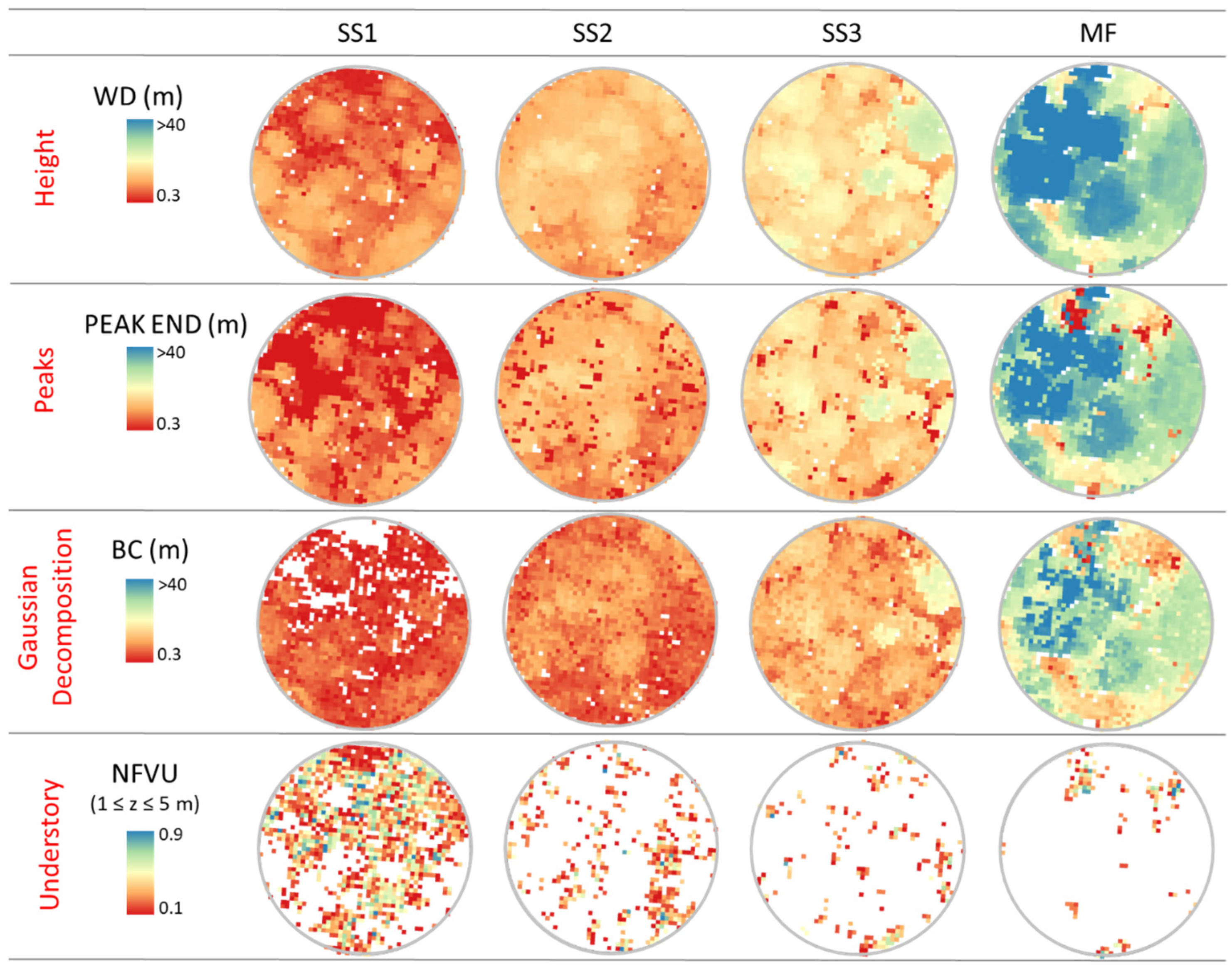
FWF metrics exhibited notable variations both within and across the circular sample plots representing various stages of secondary succession. This variability was observed in both the Drier and Wetter regions under analysis. This variability is exemplified in Figure 4, which depicts results for selected metrics representing the four categories of FWF information (Height, Peaks, Gaussian Decomposition, and Understory in Table 1). We also plotted the variability for neighboring MF sample plots situated in proximity to the secondary succession areas, which served as a local reference for comparison purposes.
From early (SS1) to advanced (SS3) stages of vegetation regrowth in the Wetter region, and extending towards the MF plot, FWF metrics like WD, PEAK END, and BC typically exhibited an upward trend, evident through shifts in color from red to yellow/blue (Figure 4). The WD, representing the waveform height or canopy top height for each voxel column, had more homogeneous values in early (SS1) and intermediate (SS2) successional stages than those observed in advanced vegetation regrowth (SS3) or Mature Forest (MF). As succession progresses, structural canopy changes make the vegetation more heterogeneous in height (SS3) until it reaches the behavior of an MF with emergent trees and clearings. The PEAK END and BC exhibited a pattern of variability akin to the WD. With the canopy structural development, the PEAK END increased towards SS3 and MF, suggesting that most of the wave energy was intercepted by the canopy, with a minimal amount reaching the ground. In relation to BC, which is a metric that relates to the first dense vegetation layer above the ground, there is a tendency for the first peak, from the ground upwards, to approach the layer of highest energy (PEAK END) with the progression of succession.
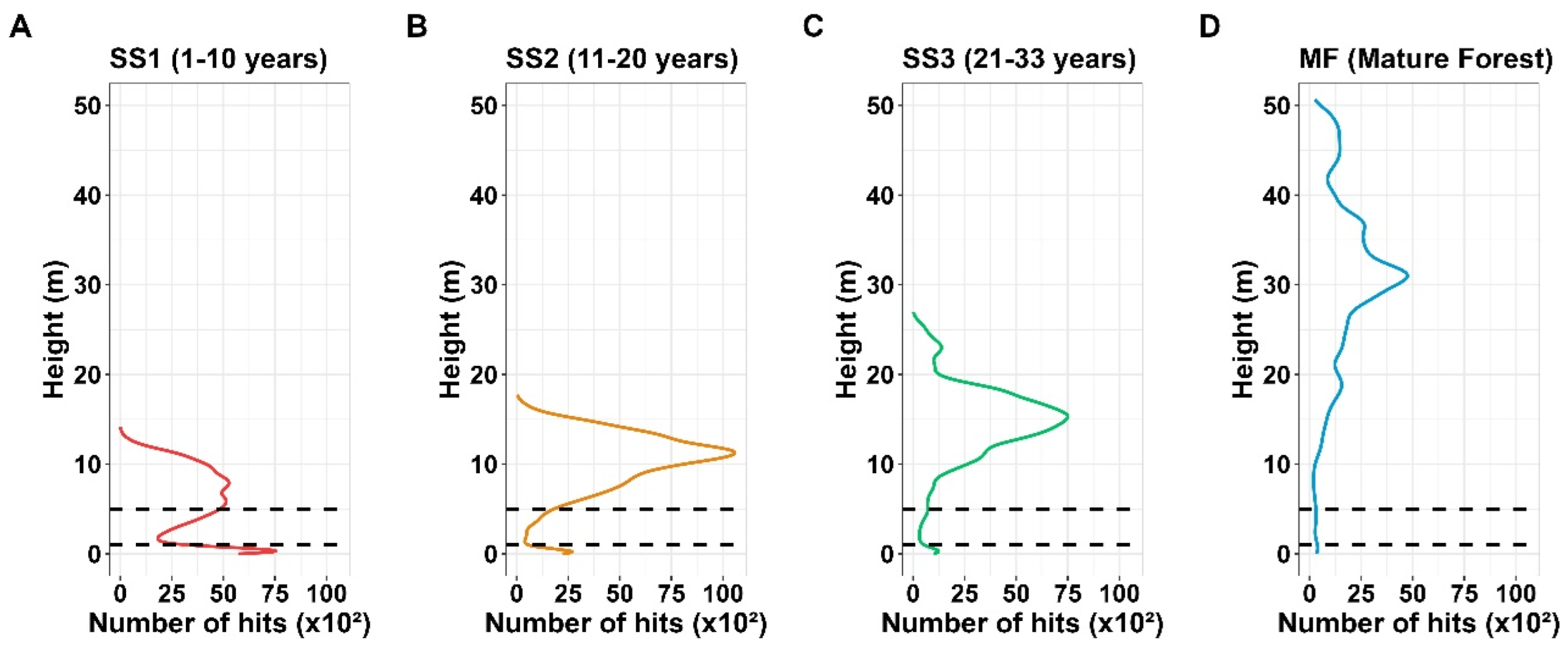
In an opposite pattern to the other metrics shown in Figure 4, the NFVU increased towards the early successional stage, representing the occupation of the understory (1 to 5 m). The NFVU does not consider the peaks but rather the proportion of voxels that contain any information on the understory. As illustrated in Figure 5, the behavior of the NFVU with vegetation regeneration is probably related to the backscatter of energy through the upper layers due to greater vegetation density. Consequently, it causes occlusion of the signal in the lower layers of the forest, which is not necessarily associated with the lack of vegetation in the understory. The number of hits between 1 and 5 m increased with decreasing canopy height from MF (Figure 5D) to SS1 (Figure 5A). Thus, there is little energy reaching the ground (0 to 1 m) and the lower stratum of the forest (1 to 5 m) with increasing height.
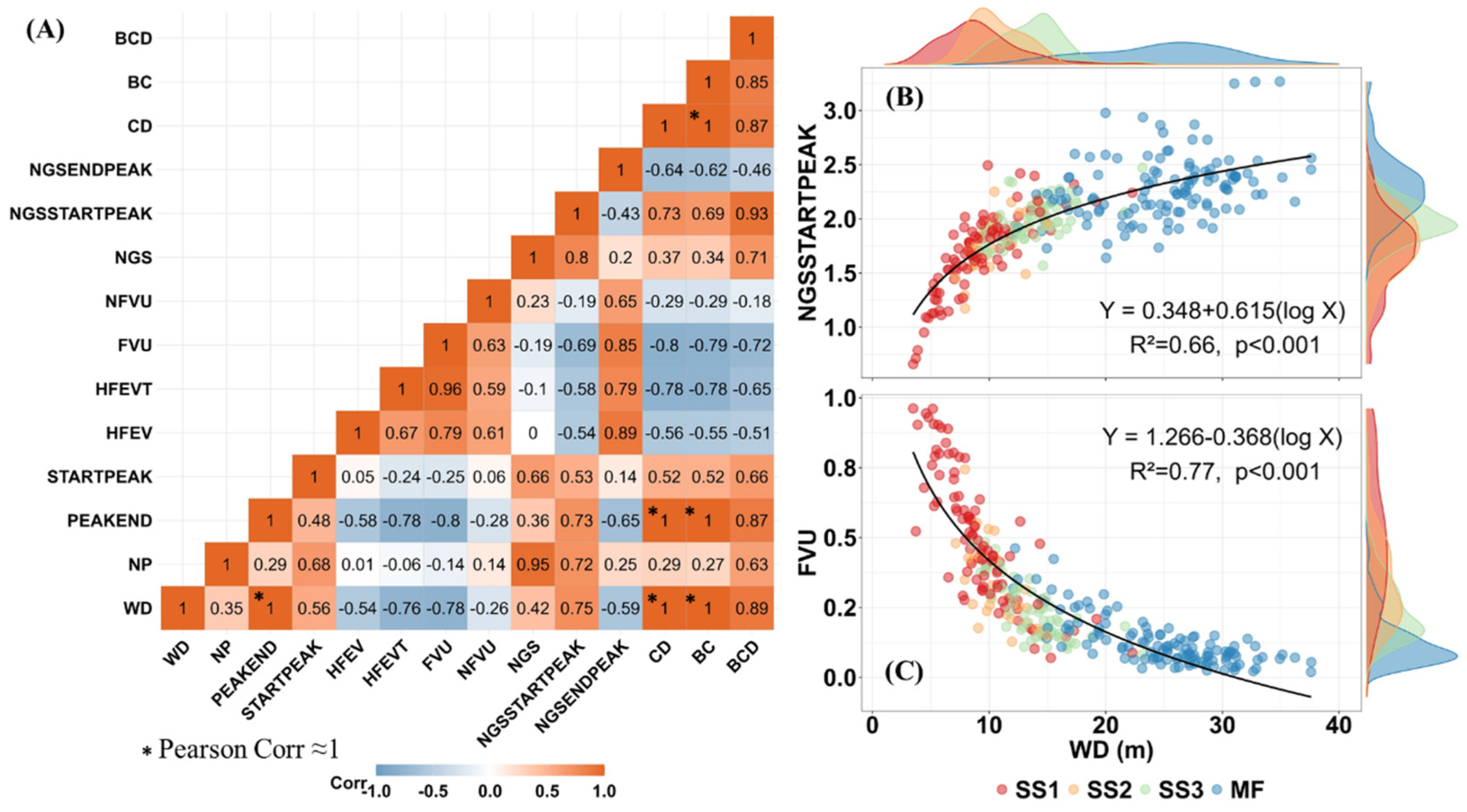
In our exploratory analysis of FWF LiDAR metrics, some of them exhibited strong correlations to each other, either negative (indicated by numbers in blue in Figure 6A) or positive (numbers in orange). For instance, negative Pearson’s correlation coefficients were observed in the relationships of FVU with PEAK END and CD (both with r = −0.80 in the correlation matrix of Figure 6A). This relationship demonstrates the reduction in energy reaching the understory with increased canopy structure. Conversely, BCD showed robust positive correlations with other metrics such as N GS STARTPEAK, BC, CD, PEAK END and WD, with correlation coefficients ranging from 0.85 to 0.89. Increasing the height and structure of the canopy, the distance between the base of the canopy and the top of the canopy tends to increase (BCD).
In Figure 6A, the presence of circular or complementary metrics is signified by correlation values close to or equal to 1. Additionally, the relationships between certain FWF metrics were not strictly linear and followed the vegetation gradient of succession, as demonstrated by the logarithmic relationships of WD with N GS STARTPEAK (Figure 6B) and FVU (Figure 6C).

3.2. Differences in FWF Metrics between Successional Stages and Climatological Regions

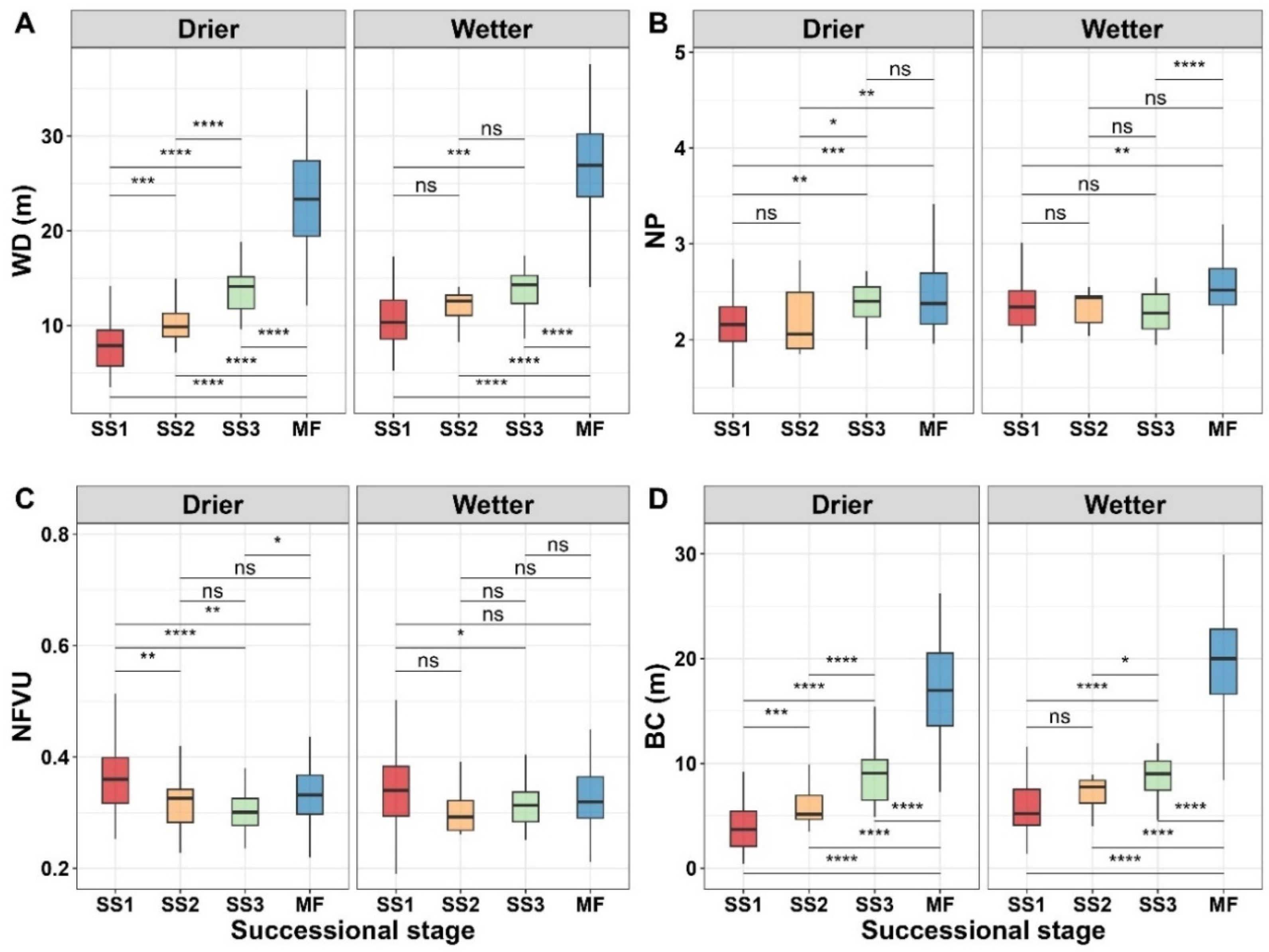
When we fixed the region (Drier or Wetter) (Table S1) and tested the statistical differences between SS1, SS2, SS3 and MF with FWF LiDAR metrics, we observed differences between some of the secondary succession stages in each region (Figure 7 and Supplementary Figure S4). For instance, the significant differences between SS1 and SS2 were observed in the Drier region for WD (Figure 7A) and BC (Figure 7D) (p < 0.001). In contrast, these two stages of vegetation regrowth did not differ statistically in both regions (p > 0.05) when using metrics like NP (Figure 7B). In the Wetter region, unlike in the Drier region, the transition from stage SS2 to SS3 did not show significant differences in the NP. However, significant increases in the NP occurred between SS1 and MF (p < 0.01) and between SS3 and MF (p < 0.0001). In the Drier region, differences between SS1 and other classes were statistically significant at different levels when the NFVU was considered in the data analysis (Figure 7C).
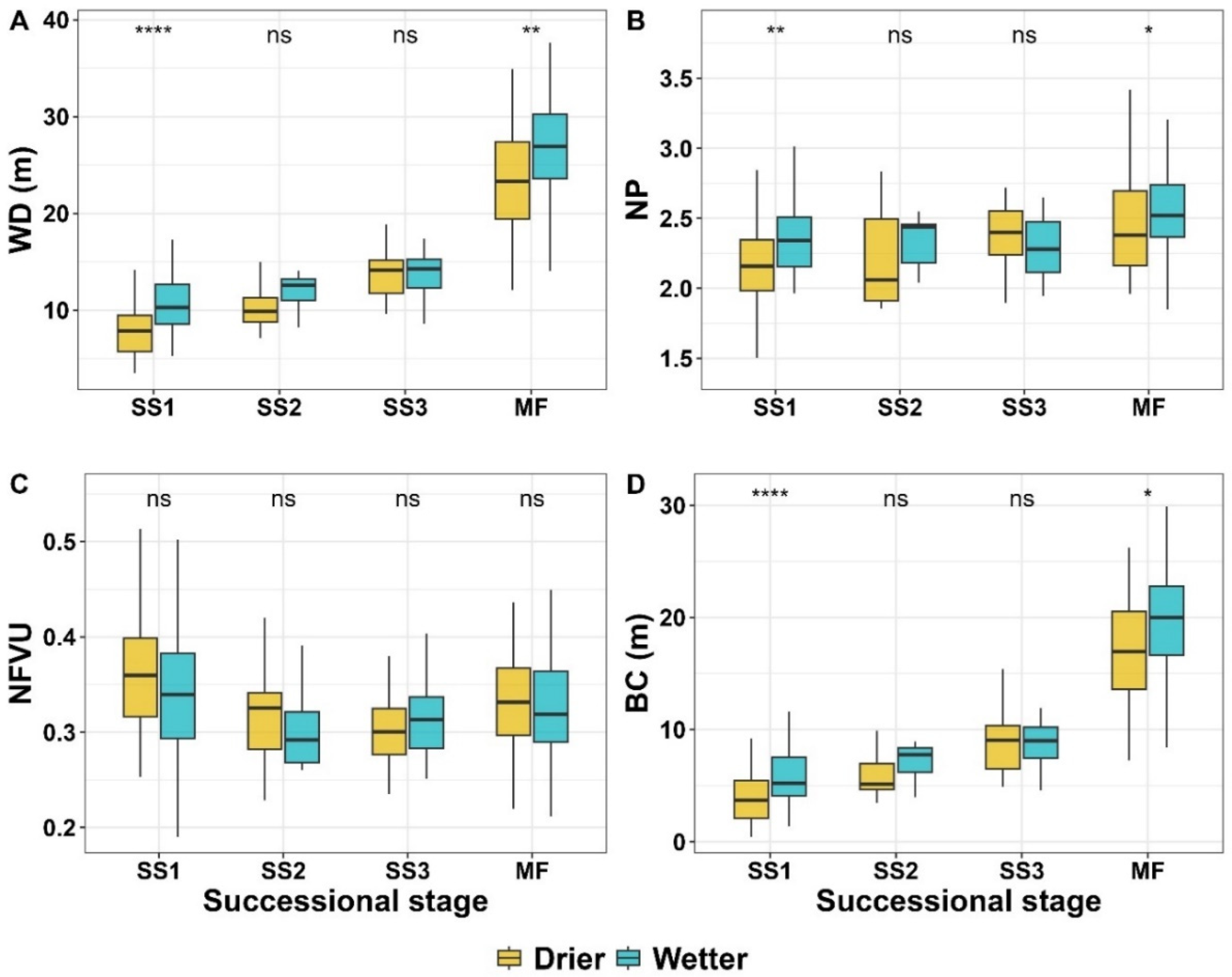
When we controlled the successional stages and examined their statistical differences in mean metrics between the Drier and Wetter regions, it became apparent that, in comparison to the Wetter region, the Drier region consistently displayed lower values of FWF LiDAR metrics like WD (Figure 8A), NP (Figure 8B), and BC (Figure 8D). Differences were more pronounced in early stages of secondary succession (SS1) with p-values ranging from 0.01 to 0.0001 (Figure 8 and Supplementary Figure S5). No significant statistical differences in means between the regions were observed for the NFVU for a given stage of vegetation regrowth (p > 0.05 in Figure 8C).

3.3. Relative Recovery of FWF Metrics with Vegetation Regrowth

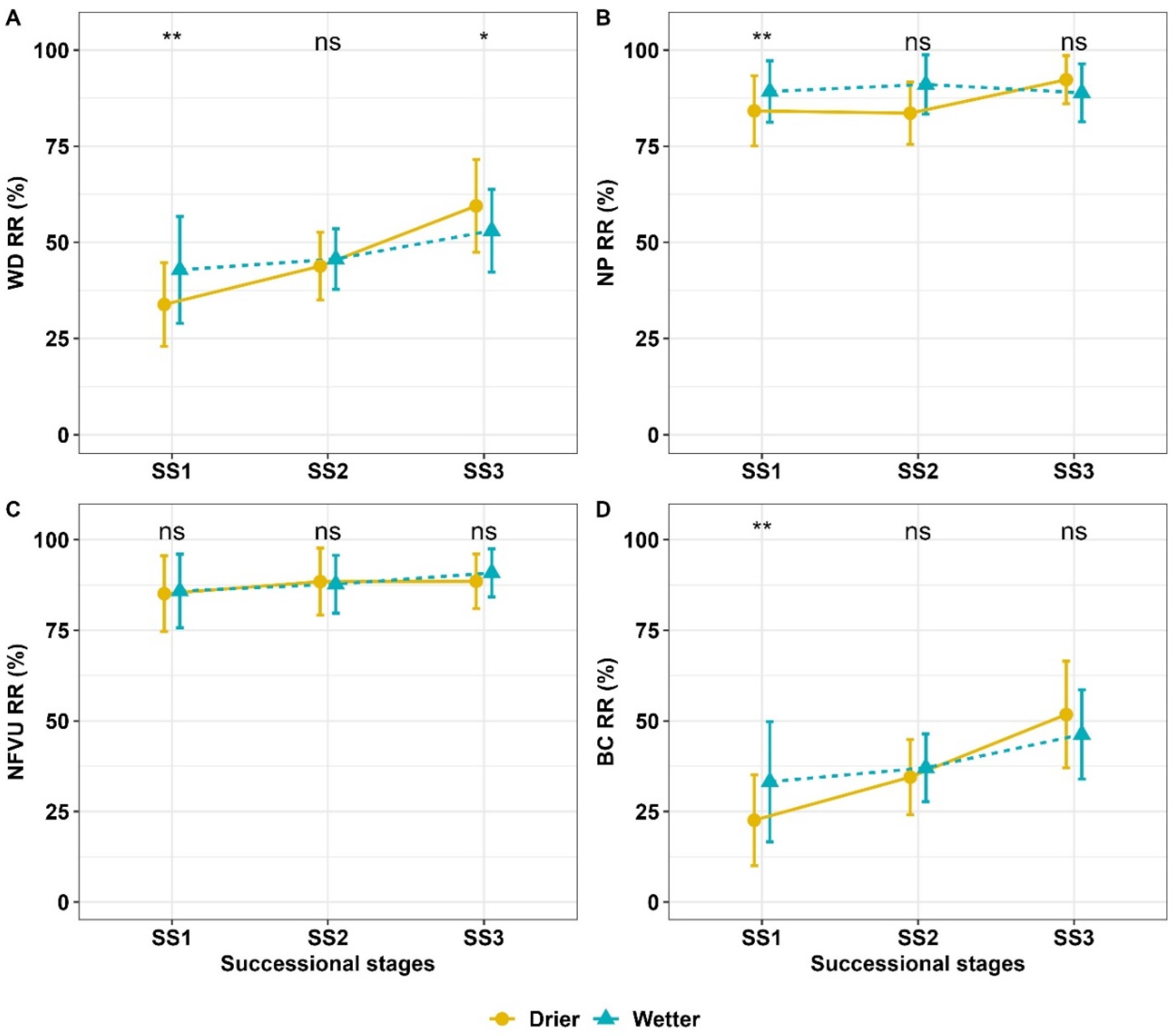
Compared to the mean values of the same metric calculated for mature forest, variable rates of relative recovery of FWF metrics were already observed in the early years of succession (SS1), ranging from 25% to 90%, as noted for BC and NP, respectively (Figure 9B–D). For both Drier and Wetter regions, these forests recovered approximately 34% and 43% of their mean height (WD) already in the SS1 stage, reaching maximum values in the SS3 stage of 53% and 60%, respectively (Figure 9A). Compared to the Drier region, the Wetter region exhibited a higher rate of relative recovery of the WD, NP, and BC metrics (Figure 9A,B,D), as well as for PEAK END, N GS STARTPEAK, CD, and BCD (Figure S5-A,G,I,J) (p < 0.01) in the early successional stage (SS1).
However, the Drier region tended to increase relative recovery (RR) rates from the SS2 stage onwards without significant differences (p > 0.05) compared to the RR of metrics of the Wetter region (Figure 9 and Supplementary Figure S6). In SS3 areas, the metrics WD, FVU, NGS, N GS STARTPEAK, and BCD showed lower RR rates for Wetter compared to Drier. This trend may be related to greater heterogeneity in terms of age and location of SS3 plots in the Wetter region, resulting in greater variability of these metrics when compared to the Drier region (Supplementary Figure S7).
Overall, we observed a trend of increasing RR rates of the metrics with the successional gradient (SS1 to SS3), except for metrics related to peak number (NP, NGS) and understory occupation (NFVU). For these metrics, the absolute mean value of successional stages approached the value found for MF, thus showing high RR or similarity with values found in MF areas and little variation across stages (Figure 9 and Figure S6).

3.4. Potential of FWF Metrics to Discriminate Stages of Secondary Succession Using Random Forest (RF)

Inspection of the RF classification results indicated the potential of FWF metrics to discriminate the stages of secondary succession. Using 14 metrics derived from LiDAR FWF data, the Drier region showed a higher overall classification accuracy (OA = 0.80) than the Wetter region (OA = 0.74) (Figure 10). It showed also higher values of Precision, Recall and F1-score than the Wetter region. For both the Drier and Wetter regions, MF and SS1 exhibited the highest values of Precision (Figure 10A) and Recall (Figure 10B), indicating less commission or false positives for the classes with extreme differences in canopy structural development. The F1-score, representing a balance between Precision and Recall, confirmed this trend in MF and SS1 areas and in the Drier region. For MF, F1-scores ranged from 0.90 to 0.96 in the Wetter and Drier regions, respectively (Figure 10C). In these regions, the lowest F1-scores (0.20 and 0.58, respectively) were recorded over SS2 areas, indicating the difficulties to discriminate this stage of secondary succession.
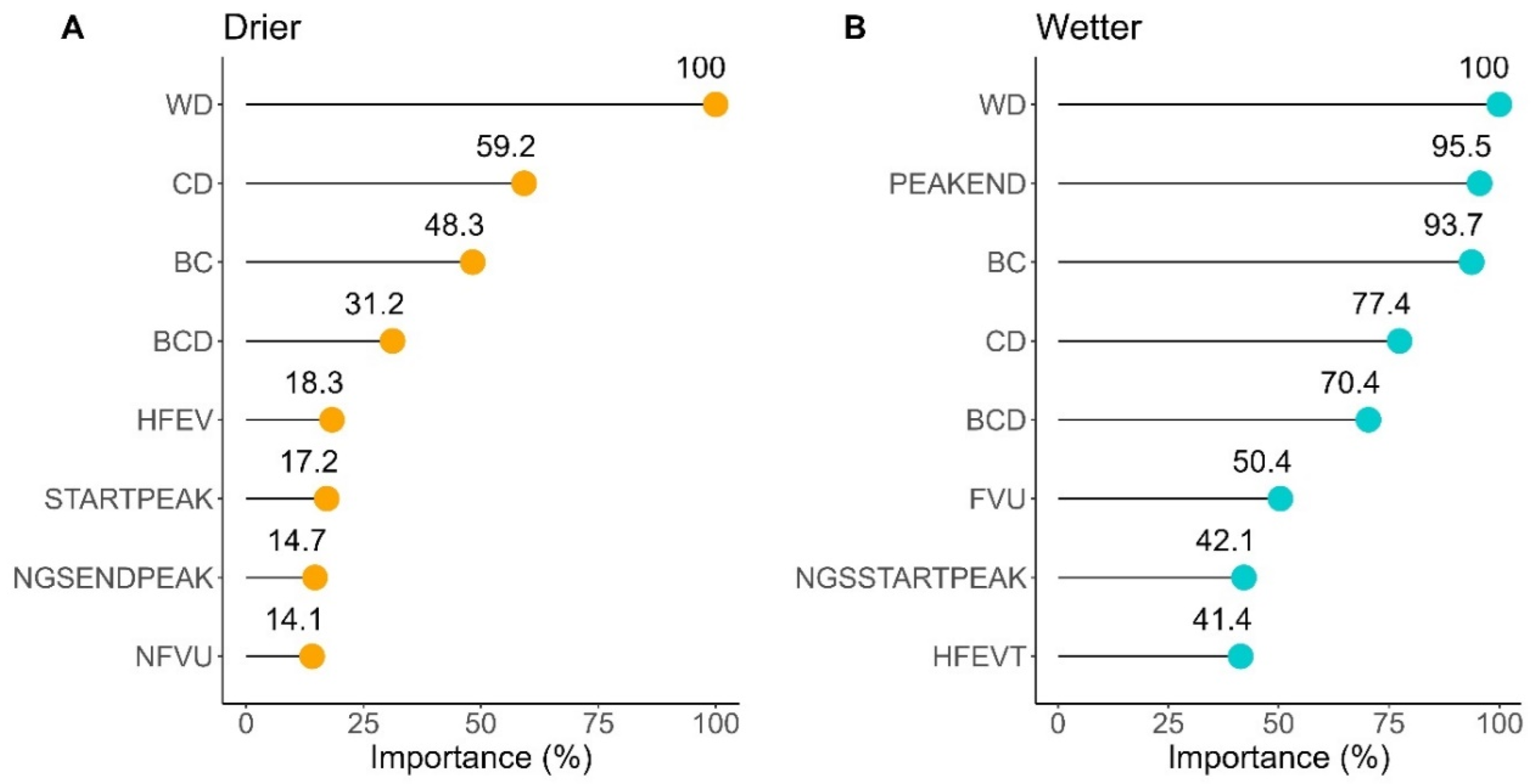
The eight most important metrics per region to discriminate MF, SS1, SS2, and SS3 are illustrated in Figure 11. In general, the WD metric, related to canopy height, was the most important metric in discriminating successional stages in both regions. In addition to WD, Gaussian Decomposition metrics such as CD, BC, and BCD, which relate to the height of the lower forest stratum, were important for both regions in different proportions but with high importance values for model performance. In the Wetter region, the number of metrics ranked with high relative importance was greater compared to the Drier region, highlighting the greater need for metrics to achieve the best classification performance. The fifth-ranked metric for the Wetter region has an importance of 70.4% (BCD) (Figure 11B), while for the Drier region, the metric occupying the same position has an importance of 18.3% (HFEV) (Figure 11A). A comparison between Figure 11A,B unveiled a more consistent set of metrics, adept at delineating differences between successional stages. These metrics, predominantly consisting of WD, CD, BC, and BCD, were consistently ranked as most important for discriminating secondary successions in both Drier and Wetter regions. Conversely, the remaining metrics demonstrated less stability in classification performance, exhibiting varying rankings in each region. The findings depicted in Figure 11 underscore the significance of FWF metrics linked to canopy height and Gaussian Decomposition in separating the stages of secondary succession within the Amazon region.

4. Discussion

Secondary forests can be understood as a continuum that involves gradual replacement or regeneration of species and populations, from an initial stage to later highly complex stages of vegetation regrowth [2]. Our study with FWF airborne data revealed significant differences in the structural modifications of canopies occurring throughout the process of secondary succession in the Brazilian Amazon. These differences, expressed by FWF metrics, depend on water availability and other coupled factors in the region, indicating distinct rates in the regeneration process of vegetation.
Overall, the Drier region showed more pronounced differences between successional stages than the Wetter region, mainly for WD, FVU, HFEVT, NGS START PEAK, CD, and BCD (Figure 7 and Figure S4). The Wetter region presented higher average values for height metrics, peaks, and Gaussian decomposition and lower average values for understory metrics, in relation to the same metrics extracted for the Drier region (Supplementary Table S1). Differences in FWF metrics between the two regions generally occur in the early stage (SS1) and mature forest (MF) (Figure 8 and Figure S4). In SS1, more significant differences were observed for WD (p < 0.0001), NP (p< 0.01), and BC (p < 0.0001) (Figure 8A,B,D). The comparative increase in precipitation results in more water availability to the plants, thereby lengthening the growing season and improving the vegetation regrowth [7,43]. With more favorable conditions for vegetation establishment, the Wetter region presented faster growth in the beginning of succession, and more homogeneous regrowth of vegetation as succession progressed. Consequently, less abrupt changes in metrics were recorded between the stages of secondary succession. As there was great growth in height in SS1, the Wetter region had a tendency of less occupation of the understory by vegetation.
Our results showed that secondary successions reached high values of relative recovery (RR) of FWF metrics in the first years of succession. RR can be a better indicator of forest resilience than analyzing its attributes in absolute values, as it refers to the percentage of the metric in that SS in relation to mature forest values under the same growth conditions [7,43]. In the Wetter region, the secondary successions recovered approximately 43% of their average height in the early stage (SS1), reaching 53% in the advanced stage (SS3). In the Drier region, a recovery of 34% and 60% was observed for SS1 and SS3, respectively. The relative recovery tends to slow down as the regeneration progresses [7]. The Wetter region showed significantly higher RR rates in SS1 for WD, NP, PEAKEND, N GS STARTPEAK, BC, BCD, and CD than in the other stages of vegetation regrowth (Figure 9 and Figure S5). However, the Drier region presented higher RR rates from the SS2 stage onwards without significant differences (p > 0.05) with the Wetter region.
Differences between climatically distinct regions should receive special attention, both with regard to the conservation of established areas and recovery through natural regeneration or active forest restoration [42]. Areas with potentially slower recovery (less water availability in the soil) may require greater interventions or long-term planning than other areas that are more likely to succeed in providing higher quality ecosystem services [7,11]. In our study, the rapid relative recovery in canopy height that reached, for instance, 45% within 20 years of vegetation regeneration in the Wetter region (Figure 9), should be carefully analyzed if associated with aboveground biomass (AGB) estimates. Poorter et al. [1] analyzed the resilience of different parameters of secondary forests in the Neotropics. They pointed out that, within 20 years after land abandonment, these areas recover, on average, about 33% of AGB compared to mature forests. However, there is a substantial gain when recovery is analyzed for another 20 years because AGB increases on average by 22%, driven also by the development of large trees, with diameter growth and not just in height.
In the classification, using RF, we obtained satisfactory results despite the reduced number of samples in some classes. The best performance was achieved for the Drier region dataset with an overall accuracy of 0.80 and a weighted F1-score of 0.80 versus an overall accuracy of 0.74 and an F1-score of 0.73 recorded for the Wetter region. We also identified mean canopy height (WD), and Gaussian decomposition metrics such as CD, BC and BCD, as the most important FWF metrics common to both regions. The analysis of these metrics deserves special attention in future studies using FWF data on secondary forests in the Amazon. The use of airborne LiDAR FWF data is widespread in the characterization of successional stages in Tropical Dry Forests using different machine learning methods [14,26,29,30]. These studies highlighted that the ecological succession process is a combination of transitional forests along a stochastic path rather than a deterministic one in nature, in which the transitions between successional stages are not considered. Duan et al. [26] demonstrated that forest transition structures vary with the main successional stages along the successional gradient. According to them, metrics based on shape (shape of the leaf area density profile) can capture this variability.
We noted that one of the potential advantages highlighted by the use of FWF data, although still underexplored in tropical regions, was a better representation of the vegetation located in the forest understory [21,22,23,44,45,46]. However, in our data, strong signal occlusion may be caused by the high and increasing density of vegetation in the canopy, generating strong backscattering of energy in the upper layers These factors may have compromised the better representation of the understory, mainly evidenced by the reduction in the FVU metric, which refers to the presence or absence of returns in the lower forest stratum (1 to 5 m) in each voxel column.
Some studies using discrete airborne LiDAR data emphasize the importance of understory metrics to differentiate forest typologies, including secondary forests, without, however, distinguishing successional stages [20,47]. However, even though dealing with discrete data, there is a high point density as well as distinct types of canopies that allow for greater beam penetration and increased possibility of intercepting vegetation within this height range (1 to 5 m). In our study, the high occupancy of the understory observed in early successional stages may be related to the presence of vegetation with high floristic diversity and importance for fauna, or by invasive species that can grow quickly over the deforested area. Understory occupancy metrics such as NFVU, FVU, and understory LAI, widely used in the literature of discrete LiDAR [47,48], indicate the occupancy and/or volume of understory vegetation, and may or may not be related to the diversity of the community in the lower forest stratum [9,20].
Our study has some limitations that should be considered in future investigations. In addition to climatological conditions, other factors affect the magnitude and sustainability of the vegetation regeneration process after land abandonment [8]. They may be coupled with the influence of precipitation or water deficit on vegetation regrowth. Here, for instance, we did not consider in our experimental design the influence of other factors such as the land-use history, forest cover and fragmentation, and soil composition and fertility. These factors can affect the vertical structure of the forest canopies and, therefore, the potential of natural regeneration to effectively restore ecosystem functions [11]. Another limitation is the lack of field inventory observations and terrestrial LiDAR surveys to reduce the uncertainties in the data analysis caused, for instance, by signal occlusion from dense vegetation of the upper canopies. The influence of the landscape configuration and intensity of the previous land-use history on vegetation recovery patterns captured by FWF metrics will be a priority in our future studies. Even the MCWD threshold adopted in our work to separate the two regions takes into consideration the number of samples representing each successional stage to ensure fair comparison between both regions. In this context, our LiDAR sampling in the Amazon did not really cover the extremes of water deficit or annual precipitation as observed, for example, in western Amazonian areas with annual precipitation exceeding 2800 mm. Therefore, differences in the behavior of FWF metrics with MCWD in the Drier and Wetter regions should be seen with care due to the coupled influence of other factors not evaluated here.

5. Conclusions

This study investigated the feasibility of employing airborne LiDAR FWF data in the Amazon region to characterize the dynamics of canopy structure modifications along the vegetation gradient from early to advanced stages of secondary successions. We examined 14 LiDAR FWF metrics derived from 309 sample plots across three groups of secondary succession (SS1, SS2, and SS3) as well as mature forest (MF). The data were obtained in two regions with distinct climatic conditions (Drier and Wetter).
Considering the three scientific questions listed before, the following conclusions were obtained:
(i)
The data analysis revealed notable differences in FWF metrics among successional stages, as well as within and between sample plots and regions. Generally, the Drier region displayed more pronounced variations between successional stages and lower FWF metric values than the Wetter region;
(ii)
In the initial stages of succession, the Drier region exhibited a slower rate of relative recovery in FWF metrics compared to the Wetter region. However, as succession progressed, the Drier region showed similar rates of recovery to those observed in the Wetter region;
(iii)
The WD metric, related to average canopy height, alongside the Gaussian Decomposition metrics (CD, BC, and BCD), associated with the lower forest stratum height, proved to be highly influential and stable in distinguishing successional stages in both analyzed regions. However, the Drier region exhibited superior discrimination between classes, achieving a weighted F1-score of 0.80, compared to 0.73 for the Wetter region.

Supplementary Materials

The Supplementary Material can be downloaded at: https://www.mdpi.com/article/10.3390/rs16122085/s1. Table S1. Mean values for each metric derived from LiDAR FWF data separated by region (Drier and Wetter) and early (SS1), intermediate (SS2) and advanced (SS3) successional stages. Values for Mature Forest (MF) are also shown for comparison. Figure S1. Spatial variations in the mean annual precipitation (1986 to 2018) and location of the 25 airborne LiDAR transects in the Brazilian Amazon region. Symbols in yellow and cyan indicate data obtained in the Drier and Wetter regions defined in the Main Text, respectively. Figure S2. Schematic representation of the differences in vegetation structure between early (SS1), intermediate (SS2) and advanced (SS3) stages of secondary succession in the Amazon region. Mature Forest (MF) is also shown as a reference of comparison. Figure S3. Empirical semivariogram and its corresponding fitted parametric model for the WD metric. The vertical dashed line indicates the distance at which the semivariance stabilized (approximately 300 meters). Figure S4. Boxplots depicting FWF metrics across successional stages categorized by climatological regions (Drier and Wetter). Asterisks denote the significance of statistical differences in means between successional stages within each region, as follows: * p < 0.05, ** p < 0.01, *** p < 0.001, **** p < 0.0001; “ns” indicates non-significant relationships. Figure S5. Boxplots depicting FWF metrics between regions (Drier and Wetter) as a function of the secondary succession stages (SS1, SS2 and SS3) and Mature Forest (MF). Asterisks denote the significance of statistical differences in means between successional stages within each region, as follows: * p < 0.05, ** p < 0.01, *** p < 0.001, **** p < 0.0001; “ns” indicates non-significant relationships. Figure S6. Relative Recovery (RR), compared to the mean values of adjacent Mature Forest (MF), for the FWF LiDAR metrics. Results are presented according to successional stages and climatological regions. Symbols and vertical bars represent mean and standard deviation, respectively. Asterisks indicate the statistical significance of metric means between the Drier and Wetter regions for each successional stage, as follows: * p < 0.05, ** p < 0.01, *** p < 0.001, **** p < 0.0001; “ns” indicates non-significant relationships. Figure S7. Density distribution of ages for different classes of early, intermediate and advanced secondary successions (SS1 to SS3), as a function of the Drier and Wetter regions defined in the Main Text.

Author Contributions

Conceptualization, A.D.J., L.S.G. and R.D.; Writing—Original Draft, A.D.J., L.S.G. and R.D.; Review and Editing, A.D.J., L.S.G., R.P.M.-N., P.C.-P., L.E.O.C.A., J.P.O., L.O.A., L.B.V., C.H.L.S.-J., A.P.L., V.P., M.A., F.R.S.P., I.H., C.T.d.A., H.L.G.C. and R.D. Supervision, L.S.G. and R.D. All authors have read and agreed to the published version of the manuscript.

Funding

This research was funded by the Conselho Nacional de Desenvolvimento Científico e Tecnológico (CNPq) (grant numbers 307792/2021-8, 141035/2021-8 and 401741/2023-0) and by the Coordenação de Aperfeiçoamento de Pessoal de Nível Superior—Brasil (CAPES)—Finance Code 001.

Data Availability Statement

The raw data supporting the conclusions of this article will be made available by the first author (Aline D. Jacon) on request.

Acknowledgments

We thank the EBA project team for providing the full-waveform LiDAR data necessary for this investigation and to Fototerra for additional information on the flight campaign. Comments by the anonymous reviewers are highly appreciated.

Conflicts of Interest

Author Henrique L. G. Cassol was employed by the company Bluebell Index. The remaining authors declare that the research was conducted in the absence of any commercial or financial relationships that could be construed as a potential conflict of interest.

References

  1. Poorter, L.; Craven, D.; Jakovac, C.C.; Van Der Sande, M.T.; Amissah, L.; Bongers, F.; Chazdon, R.L.; Farrior, C.E.; Kambach, S.; Meave, J.A.; et al. Multidimensional Tropical Forest Recovery. Science 2021, 374, 1370–1376. [Google Scholar] [CrossRef] [PubMed]
  2. Chazdon, R.L. Second Growth: The Promise of Tropical Forest Regeneration in an Age of Deforestation; University of Chicago Press: Chicago, IL, USA, 2014; ISBN 978-0-226-11807-9. [Google Scholar]
  3. Chazdon, R.L.; Broadbent, E.N.; Rozendaal, D.M.A.; Bongers, F.; Zambrano, A.M.A.; Aide, T.M.; Balvanera, P.; Becknell, J.M.; Boukili, V.; Brancalion, P.H.S.; et al. Carbon Sequestration Potential of Second-Growth Forest Regeneration in the Latin American Tropics. Sci. Adv. 2016, 2, e1501639. [Google Scholar] [CrossRef] [PubMed]
  4. Silva Junior, C.H.L.; Heinrich, V.H.A.; Freire, A.T.G.; Broggio, I.S.; Rosan, T.M.; Doblas, J.; Anderson, L.O.; Rousseau, G.X.; Shimabukuro, Y.E.; Silva, C.A.; et al. Benchmark Maps of 33 Years of Secondary Forest Age for Brazil. Sci. Data 2020, 7, 269. [Google Scholar] [CrossRef] [PubMed]
  5. Brancalion, P.H.S.; Niamir, A.; Broadbent, E.; Crouzeilles, R.; Barros, F.S.M.; Almeyda Zambrano, A.M.; Baccini, A.; Aronson, J.; Goetz, S.; Reid, J.L.; et al. Global Restoration Opportunities in Tropical Rainforest Landscapes. Sci. Adv. 2019, 5, eaav3223. [Google Scholar] [CrossRef] [PubMed]
  6. Rozendaal, D.M.A.; Bongers, F.; Aide, T.M.; Alvarez-Dávila, E.; Ascarrunz, N.; Balvanera, P.; Becknell, J.M.; Bentos, T.V.; Brancalion, P.H.S.; Cabral, G.A.L.; et al. Biodiversity Recovery of Neotropical Secondary Forests. Sci. Adv. 2019, 5, eaau3114. [Google Scholar] [CrossRef] [PubMed]
  7. Poorter, L.; Bongers, F.; Aide, T.M.; Almeyda Zambrano, A.M.; Balvanera, P.; Becknell, J.M.; Boukili, V.; Brancalion, P.H.S.; Broadbent, E.N.; Chazdon, R.L.; et al. Biomass Resilience of Neotropical Secondary Forests. Nature 2016, 530, 211–214. [Google Scholar] [CrossRef] [PubMed]
  8. Heinrich, V.H.A.; Dalagnol, R.; Cassol, H.L.G.; Rosan, T.M.; De Almeida, C.T.; Silva Junior, C.H.L.; Campanharo, W.A.; House, J.I.; Sitch, S.; Hales, T.C.; et al. Large Carbon Sink Potential of Secondary Forests in the Brazilian Amazon to Mitigate Climate Change. Nat. Commun. 2021, 12, 1785. [Google Scholar] [CrossRef]
  9. Chazdon, R.L.; Guariguata, M.R. Natural Regeneration as a Tool for Large-Scale Forest Restoration in the Tropics. Biotropica 2016, 48, 716–730. [Google Scholar] [CrossRef]
  10. Crouzeilles, R.; Beyer, H.L.; Monteiro, L.M.; Feltran-Barbieri, R.; Pessôa, A.C.M.; Barros, F.S.M.; Lindenmayer, D.B.; Lino, E.D.S.M.; Grelle, C.E.V.; Chazdon, R.L.; et al. Achieving Cost-effective Landscape-scale Forest Restoration through Targeted Natural Regeneration. Conserv. Lett. 2020, 13, e12709. [Google Scholar] [CrossRef]
  11. Jakovac, C.C.; Junqueira, A.B.; Crouzeilles, R.; Peña-Claros, M.; Mesquita, R.C.G.; Bongers, F. The Role of Land-use History in Driving Successional Pathways and Its Implications for the Restoration of Tropical Forests. Biol. Rev. 2021, 96, 1114–1134. [Google Scholar] [CrossRef]
  12. Silva, R.D.; Galvão, L.S.; dos Santos, J.R.; de J. Silva, C.V.; de Moura, Y.M. Spectral/Textural Attributes from ALI/EO-1 for Mapping Primary and Secondary Tropical Forests and Studying the Relationships with Biophysical Parameters. GIScience Remote Sens. 2014, 51, 677–694. [Google Scholar] [CrossRef]
  13. Cao, S.; Yu, Q.; Sanchez-Azofeifa, A.; Feng, J.; Rivard, B.; Gu, Z. Mapping Tropical Dry Forest Succession Using Multiple Criteria Spectral Mixture Analysis. ISPRS J. Photogramm. Remote Sens. 2015, 109, 17–29. [Google Scholar] [CrossRef]
  14. Gu, Z.; Cao, S.; Sanchez-Azofeifa, G.A. Using LiDAR Waveform Metrics to Describe and Identify Successional Stages of Tropical Dry Forests. Int. J. Appl. Earth Obs. Geoinf. 2018, 73, 482–492. [Google Scholar] [CrossRef]
  15. Becknell, J.M.; Keller, M.; Piotto, D.; Longo, M.; Nara dos-Santos, M.; Scaranello, M.A.; Bruno de Oliveira Cavalcante, R.; Porder, S. Landscape-scale lidar analysis of aboveground biomass distribution in secondary Brazilian Atlantic Forest. Biotropica 2018, 50, 520–530. [Google Scholar] [CrossRef]
  16. Almeida, C.T.D.; Galvão, L.S.; Aragão, L.E.D.O.C.E.; Ometto, J.P.H.B.; Jacon, A.D.; Pereira, F.R.D.S.; Sato, L.Y.; Lopes, A.P.; Graça, P.M.L.D.A.; Silva, C.V.D.J.; et al. Combining LiDAR and Hyperspectral Data for Aboveground Biomass Modeling in the Brazilian Amazon Using Different Regression Algorithms. Remote Sens. Environ. 2019, 232, 111323. [Google Scholar] [CrossRef]
  17. de Almeida, C.T. Integration of LiDAR and Hyperspectral Data for Forest Disturbance Characterization and Aboveground Biomass Estimation in the Brazilian Amazon; Instituto Nacional de Pesquisas Espaciais: São José dos Campos, Brazil, 2020. [Google Scholar]
  18. Martins-Neto, R.P.; Tommaselli, A.M.G.; Imai, N.N.; David, H.C.; Miltiadou, M.; Honkavaara, E. Identification of Significative LiDAR Metrics and Comparison of Machine Learning Approaches for Estimating Stand and Diversity Variables in Heterogeneous Brazilian Atlantic Forest. Remote Sens. 2021, 13, 2444. [Google Scholar] [CrossRef]
  19. Ometto, J.P.; Gorgens, E.B.; De Souza Pereira, F.R.; Sato, L.; De Assis, M.L.R.; Cantinho, R.; Longo, M.; Jacon, A.D.; Keller, M. A Biomass Map of the Brazilian Amazon from Multisource Remote Sensing. Sci. Data 2023, 10, 668. [Google Scholar] [CrossRef] [PubMed]
  20. Scheeres, J.; De Jong, J.; Brede, B.; Brancalion, P.H.S.; Broadbent, E.N.; Zambrano, A.M.A.; Gorgens, E.B.; Silva, C.A.; Valbuena, R.; Molin, P.; et al. Distinguishing Forest Types in Restored Tropical Landscapes with UAV-Borne LIDAR. Remote Sens. Environ. 2023, 290, 113533. [Google Scholar] [CrossRef]
  21. Torralba, J.; Crespo-Peremarch, P.; Ruiz, L.A. Evaluación Del Uso de LiDAR Discreto, Full-Waveform y TLS En La Clasificación Por Composición de Especies En Bosques Mediterráneos. Rev. Teledetección 2018, 27. [Google Scholar] [CrossRef]
  22. Crespo-Peremarch, P.; Tompalski, P.; Coops, N.C.; Ruiz, L.Á. Characterizing Understory Vegetation in Mediterranean Forests Using Full-Waveform Airborne Laser Scanning Data. Remote Sens. Environ. 2018, 217, 400–413. [Google Scholar] [CrossRef]
  23. Crespo-Peremarch, P.; Fournier, R.A.; Nguyen, V.-T.; Van Lier, O.R.; Ruiz, L.Á. A Comparative Assessment of the Vertical Distribution of Forest Components Using Full-Waveform Airborne, Discrete Airborne and Discrete Terrestrial Laser Scanning Data. For. Ecol. Manag. 2020, 473, 118268. [Google Scholar] [CrossRef]
  24. Marselis, S.M.; Abernethy, K.; Alonso, A.; Armston, J.; Baker, T.R.; Bastin, J.-F.; Bogaert, J.; Boyd, D.S.; Boeckx, P.; Burslem, D.F.R.P.; et al. Evaluating the Potential of Full-Waveform Lidar for Mapping Pan-Tropical Tree Species Richness. Glob. Ecol. Biogeogr. 2020, 29, 1799–1816. [Google Scholar] [CrossRef]
  25. Martins-Neto, R.P. Extraction of Structural Variables Using Lidar Data Combined with Hyperspectral Images for Classification of Upper Canopy Tree Species in Brazilian Atlantic Forest; Universidade Estadual Paulista: Presidente Prudente, Brazil, 2021. [Google Scholar]
  26. Duan, M.; Bax, C.; Laakso, K.; Mashhadi, N.; Mattie, N.; Sanchez-Azofeifa, A. Characterizing Transitions between Successional Stages in a Tropical Dry Forest Using LiDAR Techniques. Remote Sens. 2023, 15, 479. [Google Scholar] [CrossRef]
  27. Pirotti, F. Analysis of Full-Waveform LiDAR Data for Forestry Applications: A Review of Investigations and Methods. iForest 2011, 4, 100–106. [Google Scholar] [CrossRef]
  28. Crespo-Peremarch, P.; Ruiz, L.A. A Full-Waveform Airborne Laser Scanning Metric Extraction Tool for Forest Structure Modelling. Do Scan Angle and Radiometric Correction Matter? Remote Sens. 2020, 12, 292. [Google Scholar] [CrossRef]
  29. Sun, C.; Cao, S.; Sanchez-Azofeifa, G.A. Mapping Tropical Dry Forest Age Using Airborne Waveform LiDAR and Hyperspectral Metrics. Int. J. Appl. Earth Obs. Geoinf. 2019, 83, 101908. [Google Scholar] [CrossRef]
  30. Zhao, G.; Sanchez-Azofeifa, A.; Laakso, K.; Sun, C.; Fei, L. Hyperspectral and Full-Waveform LiDAR Improve Mapping of Tropical Dry Forest’s Successional Stages. Remote Sens. 2021, 13, 3830. [Google Scholar] [CrossRef]
  31. MapBiomas Project Collection 6 of the Annual Land Use Land Cover Maps of Brazil. 2021. Available online: https://mapbiomas.org (accessed on 14 February 2023).
  32. Santoro, M.; Cartus, O. ESA Biomass Climate Change Initiative (Biomass_cci): Global Datasets of Forest above-Ground Biomass for the Years 2010, 2017, 2018, 2019 and 2020, V4 2023, 5183 Files, 302039459020 B. CEDA Archive. Available online: https://catalogue.ceda.ac.uk/ (accessed on 20 April 2023).
  33. Vancutsem, C.; Achard, F.; Pekel, J.-F.; Vieilledent, G.; Carboni, S.; Simonetti, D.; Gallego, J.; Aragão, L.E.O.C.; Nasi, R. Long-Term (1990–2019) Monitoring of Forest Cover Changes in the Humid Tropics. Sci. Adv. 2021, 7, eabe1603. [Google Scholar] [CrossRef] [PubMed]
  34. Vedovato, L.B. From Past to Present: Impacts of Fire on Amazonian Forests; University of Exeter: Exeter, UK, 2022. [Google Scholar]
  35. Miltiadou, M.; Grant, M.G.; Campbell, N.D.F.; Warren, M.; Clewley, D.; Hadjimitsis, D.G. Open Source Software DASOS: Efficient Accumulation, Analysis, and Visualisation of Full-Waveform Lidar. In Proceedings of the Seventh International Conference on Remote Sensing and Geoinformation of the Environment (RSCy2019), Paphos, Cyprus, 18–21 March 2019; SPIE: Bellingham, WA, USA, 2019; Volume 11174, pp. 524–540. [Google Scholar]
  36. Hermosilla, T.; Coops, N.C.; Ruiz, L.A.; Moskal, L.M. Deriving Pseudo-Vertical Waveforms from Small-Footprint Full-Waveform LiDAR Data. Remote Sens. Lett. 2014, 5, 332–341. [Google Scholar] [CrossRef]
  37. Duong, V.H. Processing and Application of ICEsat Large Footprint Full Waveform Laser Range Data. Ph.D. Thesis, University of Technology, Delft, The Netherlands, 8 June 2010. [Google Scholar]
  38. Duncanson, L.I.; Niemann, K.O.; Wulder, M.A. Estimating forest canopy height and terrain relief from GLAS waveform metrics. Remote Sens. Environ. 2010, 114, 138–154. [Google Scholar] [CrossRef]
  39. Dalagnol, R.; Wagner, F.H.; Galvão, L.S.; Streher, A.S.; Phillips, O.L.; Gloor, E.; Pugh, T.A.M.; Ometto, J.P.H.B.; Aragão, L.E.O.C. Large-Scale Variations in the Dynamics of Amazon Forest Canopy Gaps from Airborne Lidar Data and Opportunities for Tree Mortality Estimates. Sci. Rep. 2021, 11, 1388. [Google Scholar] [CrossRef] [PubMed]
  40. R Core Team. R: A Language and Environment for Statistical Computing; R Foundation for Statistical Computing: Vienna, Austria, 2022. [Google Scholar]
  41. Brownlee, J. Imbalanced Classification with Python: Better Metrics, Balance Skewed Classes, Cost-Sensitive Learning; Machine Learning Mastery: New York, NY, USA, 2020. [Google Scholar]
  42. Kuhn, M. Building Predictive Models in R Using the Caret Package. J. Stat. Soft. 2008, 28, 1–26. [Google Scholar] [CrossRef]
  43. Toledo, M.; Poorter, L.; Peña-Claros, M.; Alarcón, A.; Balcázar, J.; Leaño, C.; Licona, J.C.; Llanque, O.; Vroomans, V.; Zuidema, P.; et al. Climate Is a Stronger Driver of Tree and Forest Growth Rates than Soil and Disturbance. J. Ecol. 2011, 99, 254–264. [Google Scholar] [CrossRef]
  44. Crouzeilles, R.; Barros, F.S.M.; Molin, P.G.; Ferreira, M.S.; Junqueira, A.B.; Chazdon, R.L.; Lindenmayer, D.B.; Tymus, J.R.C.; Strassburg, B.B.N.; Brancalion, P.H.S. A New Approach to Map Landscape Variation in Forest Restoration Success in Tropical and Temperate Forest Biomes. J. Appl. Ecol. 2019, 56, 2675–2686. [Google Scholar] [CrossRef]
  45. Ruiz, L.; Crespo-Peremarch, P.; Torralba Pérez, J. Modelling Canopy Fuel Properties and Understory Vegetation with Full-Waveform LiDAR. In Proceedings of the International Conference on Smart Geoinformatics Applications (ICSGA 2021), Prince of Songkla University, Phuket, Thailand, 24 February 2021. [Google Scholar]
  46. Crespo-Peremarch, P.; Ruiz, L.Á.; Balaguer-Beser, Á.; Estornell, J. Analyzing the Role of Pulse Density and Voxelization Parameters on Full-Waveform LiDAR-Derived Metrics. ISPRS J. Photogramm. Remote Sens. 2018, 146, 453–464. [Google Scholar] [CrossRef]
  47. Almeida, D.R.A.D.; Stark, S.C.; Chazdon, R.; Nelson, B.W.; Cesar, R.G.; Meli, P.; Gorgens, E.B.; Duarte, M.M.; Valbuena, R.; Moreno, V.S.; et al. The Effectiveness of Lidar Remote Sensing for Monitoring Forest Cover Attributes and Landscape Restoration. For. Ecol. Manag. 2019, 438, 34–43. [Google Scholar] [CrossRef]
  48. de Almeida, D.R.A.; Almeyda Zambrano, A.M.; Broadbent, E.N.; Wendt, A.L.; Foster, P.; Wilkinson, B.E.; Salk, C.; de Almeida Papa, D.; Stark, S.C.; Valbuena, R.; et al. Detecting Successional Changes in Tropical Forest Structure Using GatorEye Drone-Borne Lidar. Biotropica 2020, 52, 1155–1167. [Google Scholar] [CrossRef]
Figure 1. (A) Location of the 25 airborne LiDAR transects in the Brazilian Amazon region allocated in the Wetter (symbols in blue) and Drier (symbols in yellow) regions with MCWD greater and lower than −244.84 mm·yr−1, respectively. (B) MCWD threshold value used to allocate airborne LiDAR transects and divide counted sample plots into two regions of distinct water deficit (Drier and Wetter). (C) Number of sample plots representing each successional stage (SS1, SS2 and SS3) and Mature Forest (MF) per region (Drier in yellow and Wetter in blue).
Remotesensing 16 02085 g001
Figure 2. Process of waveform discretization, voxelization, and obtaining the pseudo-vertical waveform from maximum amplitude values in a column of voxels according to WoLFeX. Source: Adapted from Crespo-Peremarch and Ruiz [28].
Remotesensing 16 02085 g002
Figure 3. Graphical representation of the FWF LiDAR metrics extracted in WoLFeX software (v1.1.1) associated with the categories: (A) Height and Peaks, (B) Understory, and (C) Gaussian Decomposition. Source: Adapted from Crespo-Peremarch and Ruiz [28].
Remotesensing 16 02085 g003
Figure 4. Variations in selected FWF metrics (WD, PEAK END, BC, and NFVU), representing key categories of vegetation structure information (Height, Peaks, Gaussian Decomposition, and Understory), within and across circular sample plots of early (SS1), intermediate (SS2), and advanced (SS3) stages of secondary succession. The plots are located in the Wetter region. Results for adjacent Mature Forest (MF) to SS plots are also presented for comparison purposes. Metric abbreviations are defined in Table 1.
Remotesensing 16 02085 g004
Figure 5. Examples of vertical profiles depicting the number of hits in the four NFVU sample plots of Figure 4, categorized according to stages of succession: (A) Early (SS1), (B) Intermediate (SS2), (C) Advanced (SS3), and (D) Mature Forest (MF). On each graph, the dashed lines demarcate the boundaries of the understory, predefined as the region between 1 and 5 m in height.
Remotesensing 16 02085 g005
Figure 6. (A) Pearson’s correlation matrix for the relationships between the FWF LiDAR metrics, considering the entire set of successional stages and mature forest plots in the Drier and Wetter regions. Scatterplots for the non-linear log relationships of WD with N GS STARTPEAK and FVU are shown in (B,C), respectively, following the gradient from early (SS1) to advanced (SS3) stages of secondary succession, and Mature Forest (MF). The density graph for each metric is shown on the respective axes. The abbreviations of metrics are defined in Table 1.
Remotesensing 16 02085 g006
Figure 7. Boxplots depicting FWF metrics across successional stages categorized by climatological regions (Drier and Wetter). The metrics include (A) Waveform Distance (WD), (B) Number of Peaks (NP), (C) Number of Filled Voxels in the Understory (NFVU), and (D) Bottom of Canopy (BC). Asterisks denote the significance of statistical differences in means between successional stages within each region as follows: * p < 0.05, ** p < 0.01, *** p < 0.001, **** p < 0.0001; “ns” indicates non-significant relationships.
Remotesensing 16 02085 g007
Figure 8. Box plots depicting FWF metrics between regions (Drier and Wetter) as a function of the secondary succession stages (SS1, SS2 and SS3) and Mature Forest (MF). The metrics include (A) Waveform Distance (WD), (B) Number of Peaks (NP), (C) Number of Filled Voxels in the Understory (NFVU), and (D) Bottom of Canopy (BC). Asterisks denote the significance of statistical differences in means between successional stages within each region as follows: * p < 0.05, ** p < 0.01, **** p < 0.0001; “ns” indicates non-significant relationships.
Remotesensing 16 02085 g008
Figure 9. Relative Recovery (RR), compared to the mean values of adjacent Mature Forest (MF), for the FWF LiDAR metrics (A) Waveform Distance (WD), (B) Number of Peaks (NP), (C) Number of Filled Voxels at the Understory (NFVU), (D) Bottom of Canopy (BC). Results are presented according to successional stages and climatological regions. Symbols and vertical bars represent mean and standard deviation, respectively. Asterisks indicate the statistical significance of metric means between the Drier and Wetter regions for each successional stage, as follows: * p < 0.05, ** p < 0.01; “ns” indicates non-significant relationships.
Remotesensing 16 02085 g009
Figure 10. Variations in (A) Precision, (B) Recall, and (C) F1-score from Random Forest (RF) classification of samples plots located in the Drier (lines in yellow) and Wetter (lines in blue) regions, representing Mature Forest (MF), and early (SS1), intermediate (SS2), and advanced (SS3) stages of secondary succession. The Overall Accuracy (OA) is also shown for both regions. Cross validation was used to obtain the results.
Remotesensing 16 02085 g010
Figure 11. Relative importance of the top eight ranked variables for the Random Forest model classification of Mature Forest (MF) and secondary successions in the (A) Drier and (B) Wetter regions.
Remotesensing 16 02085 g011
Table 1. Description of LiDAR FWF metrics available in WoLFeX grouped by category. In this work, we adopted 1 m and 5 m as the minimum and maximum threshold values to represent possible divisions between understory and canopy, respectively.
CategoryMetric
[Reference]
Description (Units)
HeightWD
[37]
Waveform distance (m)—Distance between the beginning of the waveform and the ground or height of the waveform.
PeaksNP
[37]
Number of peaks in the waveform.
START PEAK
[38]
Distance between the beginning of the waveform and the height of maximum energy—MAX E (m).
PEAK END
[38]
Distance between the height of MAX E and the ground (m).
UnderstoryHFEV
[28]
Height of the first empty voxel from the ground upwards (m).
HFEVT
[28]
Height of the first empty voxel from a max threshold (m).
FVU
[28]
Filled voxels at the understory. Examines if there are any filled voxels between min and max threshold (Yes/No = 1/0).
NFVU
[28]
Number of filled voxels at the understory divided by the total number of voxels between min and max threshold.
Gaussian
Decomposition
N GS
[38]
Number of Gaussian curves in the waveform.
N GS STARTPEAK
[38]
Number of Gaussian curves between the beginning of the waveform and the height of the boundary.
N GS ENDPEAK
[38]
Number of Gaussian curves between the height of the boundary and the ground.
BC
[28]
Bottom of canopy: the height from the ground to the first Gaussian curve above the boundary.
BCD
[28]
Bottom of canopy distance: the distance from BC to the top of the canopy.
CD
[28]
Canopy distance: distance from the beginning of the waveform to the boundary between ground and canopy (m).
Source: Adapted from Crespo-Peremarch and Ruiz [28].
Disclaimer/Publisher’s Note: The statements, opinions and data contained in all publications are solely those of the individual author(s) and contributor(s) and not of MDPI and/or the editor(s). MDPI and/or the editor(s) disclaim responsibility for any injury to people or property resulting from any ideas, methods, instructions or products referred to in the content.