Preliminary Exploration of Coverage for Moon-Based/HEO Spaceborne Bistatic SAR Earth Observation in Polar Regions

Abstract

To address the challenge of achieving both temporal consistency and spatial continuity in Earth observation data of polar regions, this paper proposes an innovative concept of Moon-based/Highly Elliptical Orbit (HEO) Spaceborne Bistatic Synthetic Aperture Radar (MH-BiSAR), with transmitters on the Moon and receivers on HEO satellites. By utilizing ephemeris data and an orbit propagator, this study explores MH-BiSAR’s geometric coverage capabilities in polar regions and conducts a preliminary analysis of its characteristics. The findings reveal that MH-BiSAR could provide continuous multi-day revisit observations of polar regions within each sidereal month, presenting a significant advantage for monitoring high-dynamic and large-scale scientific phenomena, such as polar sea ice observations. This innovative observational method offers a new perspective for polar monitoring and is expected to deepen our understanding of polar phenomena.

1. Introduction

The polar region plays a key role in the climatology, hydrology, and energy cycles of our planet. Due to the harsh natural conditions in polar regions, there are significant obstacles to obtaining data in situ. Satellite remote sensing technology, as a powerful tool, has been widely applied in polar research, particularly with the all-day, all-weather observation capability of spaceborne synthetic aperture radar (SAR). However, spaceborne SAR systems currently operating in low Earth orbit (LEO) are constrained by observation geometry. To fully cover the entire polar region, a substantial number of images acquired at different times must be mosaiced, hindering the assurance of temporal consistency and spatial continuity in Earth observation data [1]. These limitations could impact our comprehensive understanding of large-scale polar scientific phenomena, such as sea-level rise in the context of global climate change. This encompasses events like ice shelf collapses [2], glacier variations [3], and the melting and formation of sea ice [4]. While geosynchronous Earth orbit (GSO) SAR can provide large-scale observation coverage in mid and low latitudes, its spatial coverage is limited in polar regions. Additionally, to achieve complete coverage of the polar regions, a constellation of multiple GEO satellites is required, which introduces challenges related to data temporal consistency.

The HEO is considered highly advantageous for polar observation satellites due to its significantly high apogee and ability to linger in this region for extended periods [5]. These satellites have been widely utilized for communication, optical remote sensing, and scientific research within the polar regions [6]. Simultaneously, scientists have been actively exploring the deployment of SAR on HEO satellites and have made some advancements in imaging algorithms and related areas [7,8].

Nevertheless, the implementation of HEO SAR faces numerous engineering challenges. The higher operational orbit height imposes requirements on a large antenna aperture [9], placing significant strain on satellite attitude control and orbit maintenance. Besides that, its unique orbit leads to integration time requiring hundreds of seconds or even longer, presenting significant challenges for the energy supply and thermal control of the satellite platform [10]. Furthermore, HEO satellites are subject to frequent passages through the Van Allen radiation belts, exposing them to a more complex space radiation environment than that experienced by LEO satellites. This complexity poses significant challenges to the reliability of the satellite platform and its payload [11,12]. This is particularly concerning for sophisticated and expensive systems like SAR, which are expected to have a notably reduced lifespan in HEO compared to their LEO counterparts, potentially compromising the long-term consistency of data collection. Consequently, there are currently no publicly reported HEO SAR satellites in orbit, driven by these formidable engineering hurdles.

As the Earth’s only natural satellite and the only extraterrestrial body that humans have set foot on, the Moon has received extensive attention from scientists over the past few decades. Especially in the early 21st century, with technological advancements, the world has witnessed a second wave of lunar exploration [13,14], marking a new phase in lunar exploration. Due to its tidal locking phenomenon, the Moon would be able to monitor the Earth continuously and comprehensively on a global scale. This capability will contribute to the observation of some macroscopic phenomena of the Earth, making it a promising Earth observation platform [15,16]. Its stable geological structure, vast space, and abundant energy supply provide the conditions for deploying large-aperture, high-power active sensors (such as SAR). Additionally, through effective maintenance by technical personnel stationed at Lunar bases, the Moon-based observation platform is expected to achieve a lifespan far exceeding that of artificial satellite platforms, ensuring the long-term consistency of data. However, the significant transmission loss caused by the long distance between the Earth and the Moon adversely affects the signal-to-noise ratio (SNR) of imaging, especially in scenarios involving observations of high-latitude regions of the Earth with large incident angles [17,18].

In recent years, due to its unique advantages, the bistatic synthetic aperture radar (BiSAR) has gained increased attention. With advancements in both theoretical and engineering aspects of BiSAR, a growing number of BiSAR systems have been deployed [1,19,20]. Furthermore, several concepts of BiSAR based on high-orbit radiation sources have also been proposed [21,22]. Therefore, a bistatic configuration has been proposed that entails deploying the transmitter at a Moon-based observatory and the receiver on satellites orbiting at medium to high altitudes, to facilitate large-scale Earth observations [23]. Through a well-designed orbit for the receiving satellite, this configuration can enhance the observational performance over designated regions and significantly reduce the transmission power required for Moon-based SAR Earth observations. This, in turn, notably decreases the initial construction costs of a Moon-based observatory. Additionally, the obtained bistatic scattering data can also provide additional information for terrain parameter inversion.

By deploying high-power transmitters and large-aperture antennas on a Moon-based observatory to form a BiSAR, the complexity of the payload on HEO satellites can be significantly reduced and its reliability can be improved. Figure 1 shows the conceptual illustration of MH-BiSAR for Earth’s polar regions observation. Compared to costly monostatic HEO SAR, MH-BiSAR substantially reduces the funding requirements for HEO SAR satellites while improving their reliability. In addition, there is potential to further reduce costs by integrating HEO satellites with polar communication services.

In this paper, we conducted an exploratory preliminary analysis of the observation coverage of a special bistatic SAR configuration called MH-BiSAR, based on the observation geometry. In Section 2, we introduced the dynamic characteristics of the Moon and the HEO Satellites (taking Molniya Orbit as an example). The observation geometric model and its constraints were also presented. In Section 3, we calculated the observation coverage of MH-BiSAR for polar regions using the Moon-Based/Spaceborne BiSAR (MS-BiSAR) Earth observation geometric model and discussed its characteristics, with a preliminary discussion on the observation coverage of polar sea ice. Section 4 and Section 5 analyzed some limitations of this study and discussed the challenges and further research plans for MH-BiSAR. Section 6 concludes the paper.

2. Observation Geometry

To evaluate the coverage characteristics of MH-BiSAR in polar regions observation, it is essential to analyze the observational geometry involving the Moon, HEO satellites, and Earth. In this paper, we used the DE430 ephemeris [24] to obtain the position and attitude information of the Moon. The Simplified Deep-Space Perturbations-4 (SDP4) orbit propagator is employed to simulate the satellite orbits. Additionally, Earth orientation parameters (EOP) are used for the reference system transformation [25].

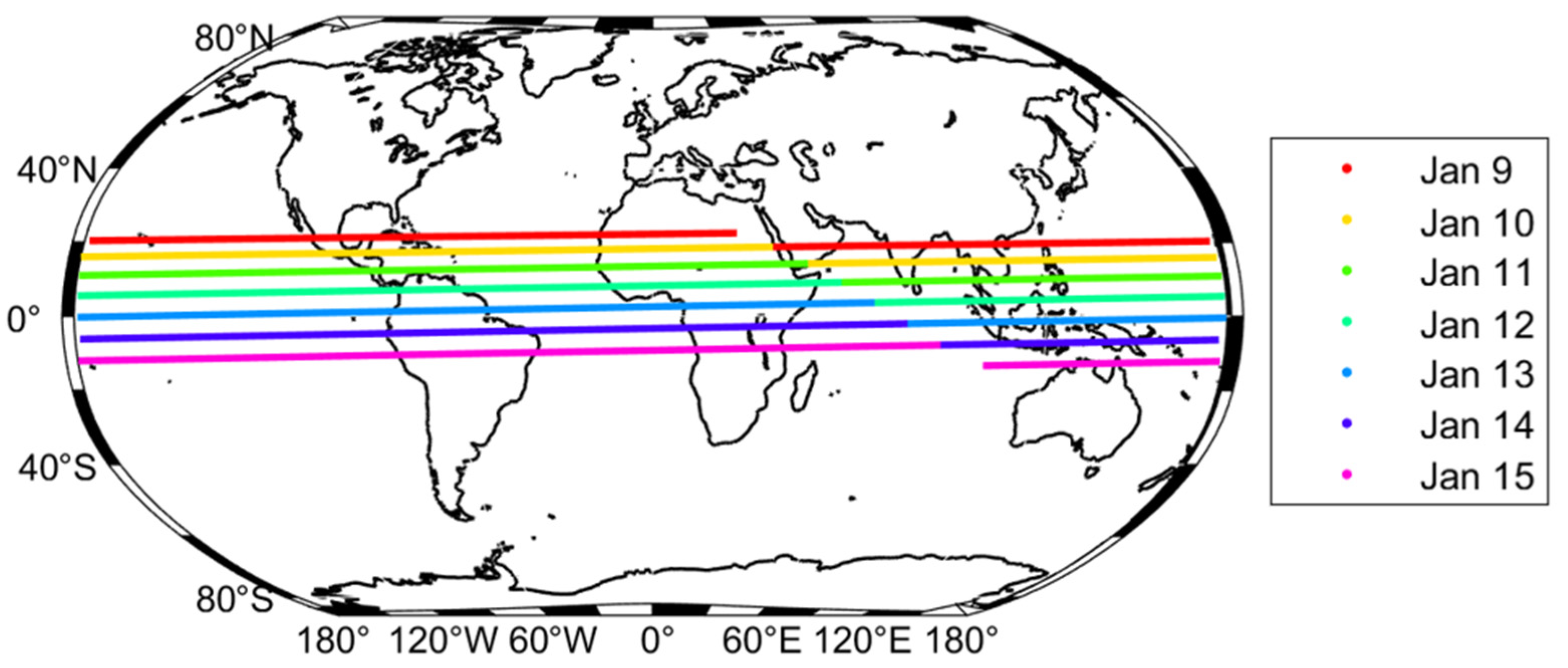
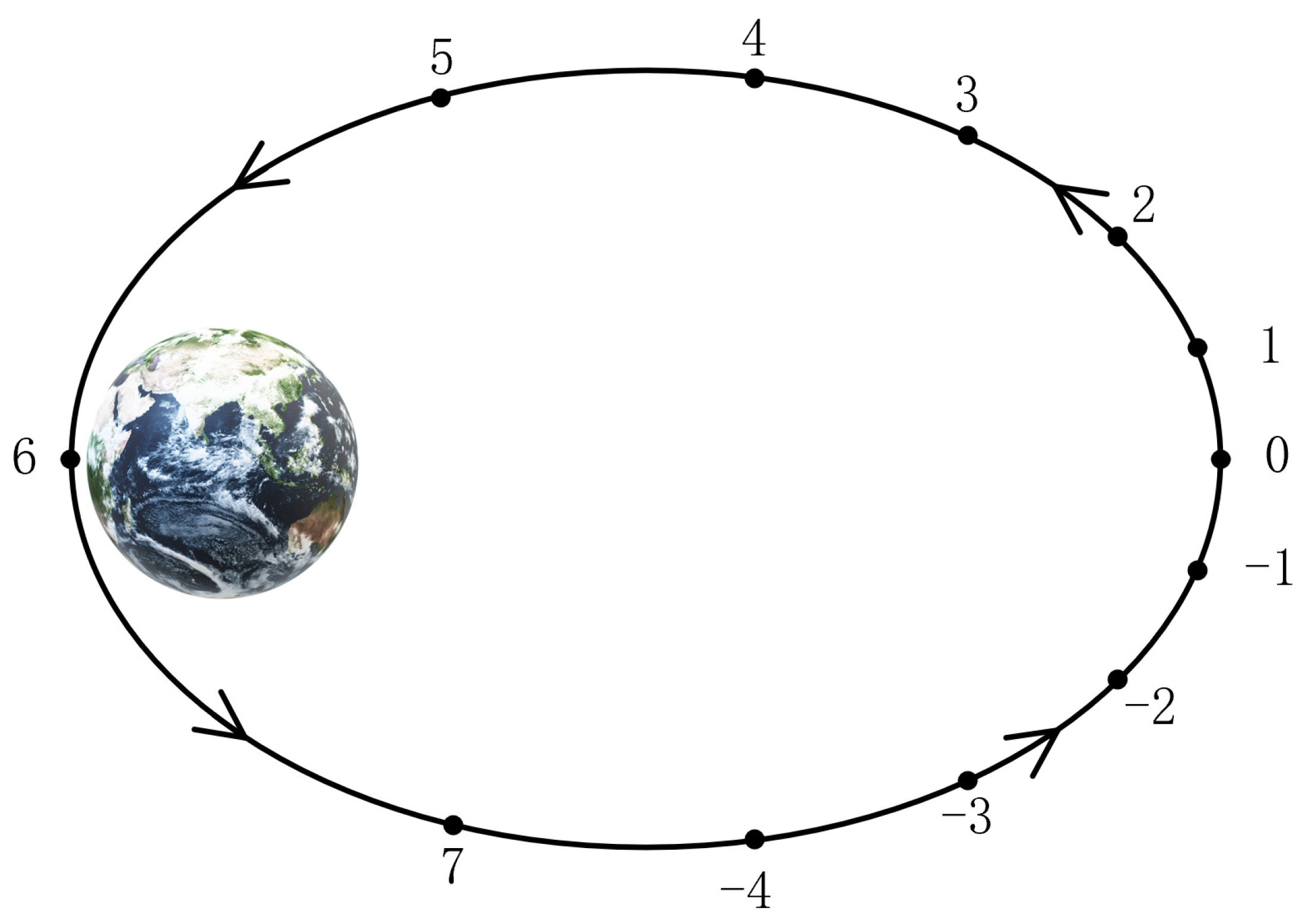
2.1. Dynamics of the Moon and HEO Satellites

To better analyze the geometric observations of MH-BiSAR, a brief overview of the dynamic characteristics of the Moon and HEO satellites is provided. As Earth’s natural satellite, the Moon orbits the Earth along an elliptical path, with an average semi-major axis of 384,748 km, an average eccentricity of 0.0549, and an orbital period of approximately 27.32 days (a sidereal month). Due to tidal locking, the Moon’s rotation period matches its orbital period around the Earth. Consequently, one side of the Moon continuously faces Earth. This unique rotation state enables sensors deployed on the side facing Earth to achieve continuous observation of our planet, making the Moon an ideal remote sensing platform.

Simultaneously, due to the gravitational influence of the Sun and Earth, the Moon’s orbit experiences short-term cycles (27.32 days) and long-term cycles (18.6 years). This also results in corresponding long and short periodic variations in the observation coverage of different regions on Earth by the Moon-based observatory.

As depicted in Figure 2, the tracks of the sublunar point on the Earth’s surface are illustrated over a week (from 9 to 15 January 2023). It is notable that within a single day, the longitudinal variation of the nadir point can exceed 340°. Therefore, for most regions that can be covered, the revisit time of the Moon-based observatory is less than one day. In contrast to the longitudinal variation, the latitude changes minimally within a single day (around 3°) [26]. Figure 3 shows the variation of the sublunar points within one orbital period (sidereal month). On the one hand, it can be observed from the figure that the latitude of the sublunar points follows a sinusoidal wave-like pattern, with the equator as the central line, oscillating between maximum and minimum values. On the other hand, the longitude undergoes a complete cycle of variation within each day.

From Figure 4, it can be observed that the maximum values of latitude fluctuate on an inter-annual basis. In the northern hemisphere, the maximum latitude fluctuates between 18.5° and 28.7°, while in the southern hemisphere, it fluctuates between the same values. These fluctuations exhibit a stable period of approximately 18.6 years, which corresponds to the variation period of the angle between the lunar orbital plane and the Earth’s equatorial plane (lunar nodal period). These long-term cyclic variations in the latitude of the sublunar points lead to the long-period characteristics of coverage for Moon-based observatories on Earth.

Unlike the circular or near-circular orbits used by most current spaceborne SAR systems, HEO has a larger eccentricity, resulting in a high apogee and a low perigee. Among these, a typical HEO is the Molniya orbit, extensively utilized for satellite orbits providing communication and remote sensing services in high-latitude regions. The orbit parameters are outlined in

Table 1. Molniya orbit parameters.

Parameter	Value
Semi-major axis (km)	26,500
Argument of Perigee (deg)	270
Eccentricity	0.741
Inclination (deg)	63.4
Perigee altitude (km)	~600
Apogee altitude (km)	~39,750
Orbital period (day)	~0.5
Orbital revisit period (day)	~1

, and the definition of the orbital parameters can be found in Figure 5 [27].

The orbital parameters of the Molniya Orbit reveal it has substantial inclination and eccentricity. This allows its nadir point to reach high-latitude regions on Earth. Additionally, with an apogee altitude close to 40,000 km (comparable to a GSO), it enables large-scale instantaneous coverage of the Arctic. Figure 6 shows the Molniya orbit as viewed perpendicular to the orbital plane. According to Kepler’s laws, the satellite moves very slowly near apogee and rapidly near perigee, enabling continuous monitoring possibilities for the polar regions.

Meanwhile, for comparable coverage over the Antarctic region, the apogee can be positioned in the high latitudes of the Southern Hemisphere. This configuration is known as an inverted Molniya orbit, which features an Argument of Periapsis of 90° [28], as depicted by the red track in Figure 7. The utilization of these two satellites enables enhanced daily coverage of both the Arctic and Antarctic regions. In order to further analyze the observation coverage of MH-BiSAR, in this paper, we select a Molniya orbit satellite and an inverted Molniya orbit satellite for receiver deployment. Both satellites, when paired with a Moon-based transmitter, form an MH-BiSAR to achieve coverage over the Arctic and Antarctic regions, respectively.

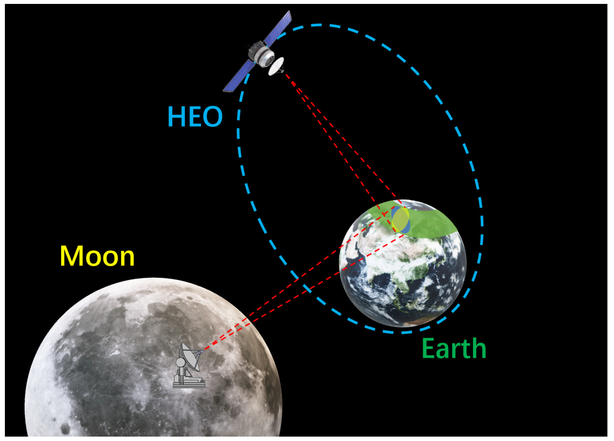
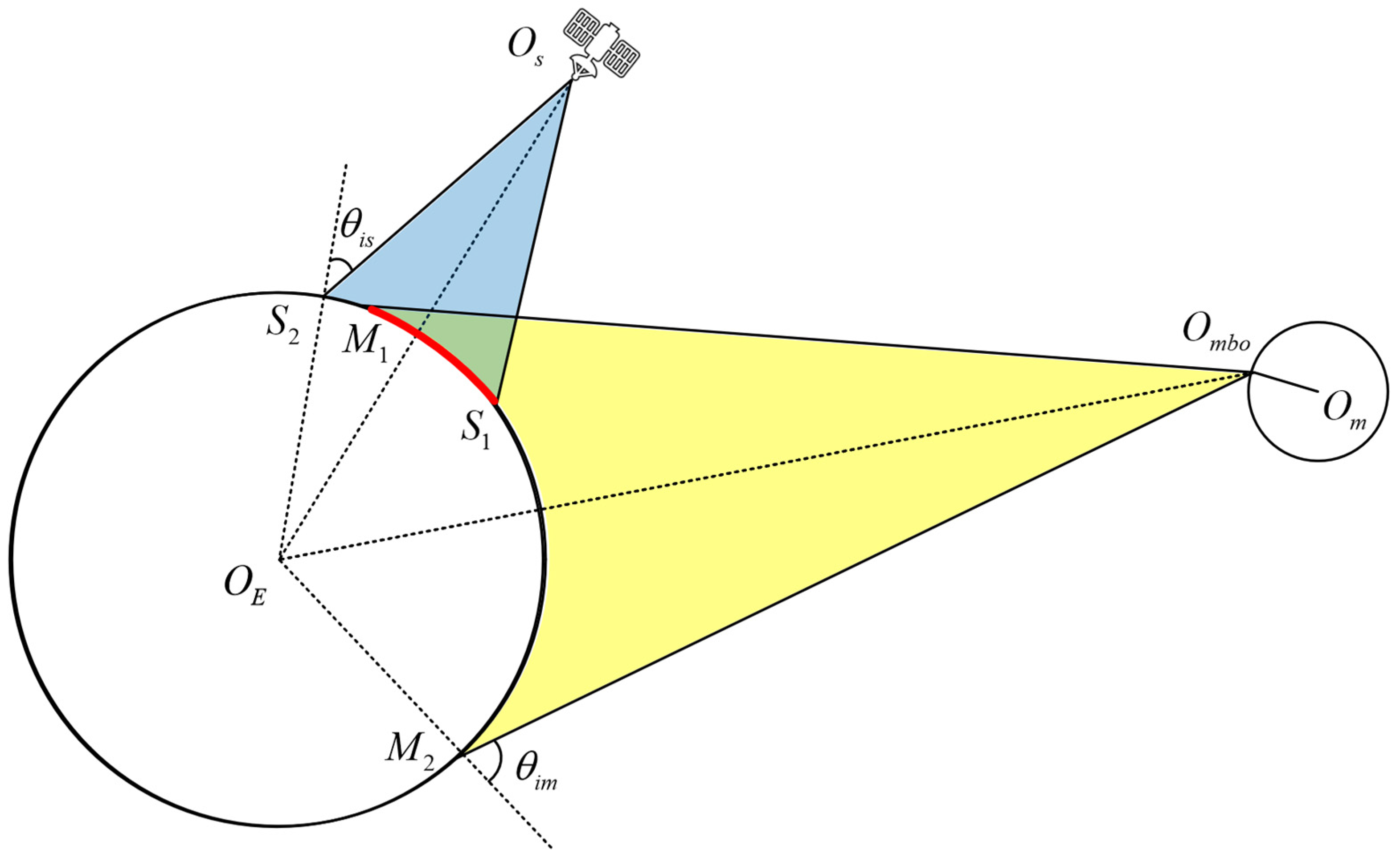
2.2. Observation Geometric Model

This paper employs the simplified MS-BiSAR Earth observation geometrical model to determine the Earth observation coverage of MH-BiSAR, as depicted in Figure 8 [23]. By utilizing ephemeris, EOP data, and satellite orbit propagator, and unifying the reference systems, the precise geometric relationships among the Moon, satellite, and Earth are established.

The incidence angle is a constraint parameter determined in this study for Earth observation coverage, aimed at avoiding situations where the SNR of the echo becomes too low under high incidence angle conditions, making imaging unfeasible. Unlike monostatic SAR, for MH-BiSAR, the SNR of the bistatic scattering echoes is related to the positions of both the Moon-based observatory and satellite.

We defined the coordinates of the Moon-based observatory $O_M\left(X_M,Y_M,Z_M\right)$, the satellite $O_s\left(X_s,Y_s,Z_s\right)$, the target on the Earth $T\left(X_T,Y_T,Z_T\right)$, and the barycenter of the Earth $O_s\left(0,0,0\right)$.

The incidence angle of the transmitter ${\theta }_m$ and the receiver ${\theta }_s$ are as follows:

$${\theta }_m=\mathit{arccos}\left(\frac{\left(X_M-X_T\right)X_T+\left(Y_M-Y_T\right)Y_T+\left(Z_M-Z_T\right)Z_T}{\sqrt{\left({\left(X_M-X_T\right)}^2+{\left(Y_M-Y_T\right)}^2+{\left(Z_M-Z_T\right)}^2\right)\left(X_T^2+Y_T^2+Z_T^2\right)}}\right)$$

(1)

$${\theta }_s=\mathit{arccos}\left(\frac{\left(X_S-X_T\right)X_T+\left(Y_S-Y_T\right)Y_T+\left(Z_S-Z_T\right)Z_T}{\sqrt{\left({\left(X_S-X_T\right)}^2+{\left(Y_S-Y_T\right)}^2+{\left(Z_S-Z_T\right)}^2\right)\left(X_T^2+Y_T^2+Z_T^2\right)}}\right)$$

(2)

In previous studies on Moon-based monostatic SAR, the maximum threshold for the incidence angle is typically set at 60° to satisfy the SNR requirements [26,29]. Due to the geometry of Moon-based SAR observations, observations of polar targets often face challenges with larger incidence angles. In this paper, to enhance the SNR of the received echoes, we set the maximum threshold for the incidence angle of the satellite receiver at 40°. Considering the characteristic that electromagnetic waves attenuate with the square of the distance, and that the apogee of the Molniya orbit is only about one-tenth of the Earth–Moon distance, deploying the receiver on the satellite significantly reduces transmission losses (by approximately two orders of magnitude). We set the maximum threshold for the Moon-based transmitter’s incidence angle at 70° for better coverage of polar regions. Therefore, when $0<{\theta }_m<70°$ and $0<{\theta }_s<40°$ the target on the Earth is observable.

3. Coverage Characteristics of Polar Regions

Once the precise geometric relationship between the Moon, satellite, and Earth is established, the observation geometric model can be employed to determine Earth observation coverage of MH-BiSAR and discuss the characteristics of the coverage. As the Earth observation coverage of a bistatic SAR is determined by both the transmitter and receiver platforms, this section begins with an overview of the Earth observation capabilities of Moon-based and HEO satellite platforms. Then, we use the Simplified MS-BiSAR Earth observation geometric model to calculate and analyze its coverage of BH-BiSAR.

3.1. Coverage Characteristics of Moon-Based and HEO Platforms

To further evaluate the platform’s coverage across various locations within the polar regions, sample points were selected to calculate the platform’s coverage time. Previous studies have shown that the Moon-based platform’s coverage characteristics of various latitude regions in the northern and southern hemispheres within one sidereal month are symmetric about the equator, while the Molniya orbit and inverted Molniya orbit are symmetric about the equatorial plane. Therefore, in this section, we mainly analyze the platform’s coverage of sample points in the Arctic region. The locations of these sample points are as follows: (90°N), (85°N, 0°), (85°N, 90°E), (85°N, 180°), (85°N, 90°W), (75°N, 0°), (75°N, 90°E), (75°N, 180°), (75°N, 90°W), (65°N, 0°), (65°N, 90°E), (65°N, 180°), (65°N, 90°W).

Under the constraint of a 70° incidence angle threshold, the Moon-based observatory’s coverage of these sample points within one sidereal month (1 to 28 January 2023) is shown in Figure 9. In this figure, different colors represent the longitudes of the sampling points, while the vertical axis is divided into four regions representing the latitudes (90°N, 85°N, 75°N, 65°N) of the sampling points. The horizontal lines indicate the time span during which the point can be observed by the platform.

It can be observed that over the course of a sidereal month, the Moon-based platform is able to conduct daily observations of various sampling points across the Arctic for several consecutive days. However, its observational capabilities vary for sample points at different latitudes. Specifically, sampling points at the North Pole and 85°N experience extended continuous coverage, while lower latitude regions within the Arctic experience more frequent revisits within a month (13 revisits for the 75°N sampling point, and 16 revisits for the 65°N sampling point). This implies the ability to achieve more consecutive daily revisits over more days, and the coverage duration for each sampling point is relatively uniform on most days, with only slight decreases at the beginning and end. Compared to the impact of latitude, the sampling points’ longitude variations have a minimal effect on coverage duration and frequency.

Figure 10 illustrates the observable spans of the Arctic by the HEO platform, with an incidence angle threshold set to 40°. It is evident that due to its orbital revisit period of 24 h, meaning its nadir track is repeatable over a 24-h period, there are no differences in daily observation duration and frequency for the sampling points. Additionally, the Molniya orbit can achieve daily observation coverage for all sampling points in the Arctic, with twice-daily observations possible for the 90°N and 85°N sampling points. However, since the nadir points for the HEO platform do not uniformly change like the Moon-based platform, there are differences in observation duration for sampling points at different longitudes. To enhance the continuous observation coverage time for specific longitude sampling points, it is necessary to adjust the ascending node longitude of the satellite orbit to achieve a suitable longitude of the nadir point at the apogee, it should be noted that although there are differences in observation duration, at least daily revisits are achievable for different sampling points.

To achieve more consistent observation coverage across different longitudes in the polar regions, a two-satellite system on the Molniya Orbit has been proposed [30]. The nadir track of this system is illustrated in Figure 11. This configuration employs two satellites in the same orbital plane, staggered by half an orbit in their perigee passages. As illustrated in Figure 12, this approach enhances the coverage uniformity across the Arctic region’s longitudes.

3.2. Coverage Characteristics of MH-BiSAR

For MH-BiSAR, we employed the Molniya orbit as the receiving satellite’s operational orbit and evaluated its coverage of sampling points using a bistatic incidence angle threshold, as depicted in Figure 13.

It can be observed that due to the daily revisit characteristics of the Molniya orbit, the number of days that sampling points can be observed is primarily determined by the Moon-based platforms. Simultaneously, it is evident that there are significant differences in the daily continuous observation time for different longitude targets at 65°N and 75°N, mainly influenced by the visibility of the targets by the HEO satellites. As mentioned earlier, adjusting the longitude of the satellite’s ascending node on the ground can enhance the observation duration for specific longitude targets. Furthermore, in terms of observation frequency, MH-BiSAR achieves a minimum daily revisit of 7 days, 9 days, 12 days, and 11 days for sampling points at 90°N, 85°N, 75°N, and 65°N, respectively. Moreover, for certain longitude targets at 65°N, observation coverage of over 14 days can be achieved.

Figure 14a,b provide a visual representation of the daily cumulative observable time achieved by MH-BiSAR for the Arctic and Antarctic regions, respectively, within one sidereal month.

Within a single sidereal month, it can be observed that MH-BiSAR exhibits variations in the cumulative daily observation duration for high-latitude regions in the Northern Hemisphere. For the majority of the Arctic, there are extensive continuous observation windows of approximately 8 days, with at least 6 days offering more than 8 h of observation time daily. In the 70°N to 80°N latitude range, even longer cumulative daily observation durations are achieved. As previously mentioned, it can also be noted that there are differences in cumulative observation time across different longitudes in the polar regions. Similar patterns can be observed in the Antarctic region.

It should be noted that the analysis provided here only qualitatively reflects the observation characteristics of MH-BiSAR for polar regions, as the orbital design of the receiving satellite in the Molniya orbit was not optimized based on specific observation mission requirements. For different observation missions, the observation capabilities for specific regions can be further enhanced through appropriate satellite orbit design.

To analyze the coverage variations over long periods, calculations are conducted on the annual accumulated observable time for the MH-BiSAR in a lunar nodal cycle, presented in

Table 2. Annual accumulated observable time of MH-BiSAR for different sample points in one Lunar Precession Period.

Sample Points	Annual Accumulated Observable Time (Hours)																			CV
	2005	2006	2007	2008	2009	2010	2011	2012	2013	2014	2015	2016	2017	2018	2019	2020	2021	2022	2023
(90°N)	6039	6178	6331	6389	5348	4945	4499	3735	2862	290	0	0	0	0	0	1673	3292	4756	5419	0.781
(85°N, 0°E)	5696	5925	6075	6090	5101	4641	3944	3101	2766	2081	1596	1255	1075	1227	1679	2121	2817	4102	5010	0.518
(85°N, 90°E)	5334	5559	5706	5734	4828	4360	3710	2961	2655	1959	1418	1238	941	1100	1623	1956	2640	3854	4688	0.521
(85°N, 180°)	5599	5790	5980	6026	5042	4539	3832	3049	2756	2041	1556	1221	1069	1218	1671	2088	2717	4058	4910	0.518
(85°N, 90°W)	5428	5622	5778	5847	4895	4381	3754	3022	2671	2039	1462	1267	960	1093	1654	2014	2704	3923	4732	0.518
(75°N, 0°)	4104	4145	4231	4233	3618	3490	3288	3061	3256	2997	2848	2860	2593	2510	2725	2693	3000	3563	3748	0.174
(75°N, 90°E)	3968	3845	3936	4094	3409	3327	3208	2883	3082	2847	2548	2750	2308	2245	2667	2486	2790	3485	3494	0.185
(75°N, 180°)	4122	4115	4231	4241	3620	3488	3298	3089	3263	3006	2850	2872	2591	2504	2722	2691	2972	3574	3730	0.173
(75°N, 90°W)	3939	3874	3929	4110	3396	3270	3238	2891	3063	2871	2552	2731	2336	2252	2668	2476	2755	3499	3481	0.184
(65°N, 0°)	2064	2001	2143	2040	1824	1878	1708	1671	1904	1716	1767	1831	1645	1655	1661	1577	1740	1840	1901	0.088
(65°N, 90°E)	4974	4773	4838	5029	4297	4286	4290	3993	4377	4277	3983	4322	3851	3694	4067	3722	3965	4597	4481	0.093
(65°N, 180°)	2088	1995	2116	2063	1837	1866	1717	1676	1896	1717	1749	1846	1633	1650	1660	1573	1732	1833	1898	0.089
(65°N, 90°W)	4968	4789	4810	5044	4317	4259	4305	4011	4332	4300	3988	4297	3866	3686	4061	3732	3931	4628	4493	0.093

. The results indicate significant differences in accumulated observable time for various sampling points across different years. By calculating the coefficient of variation (CV) of the annual accumulated observable time, it is found that interannual variability is more pronounced in high-latitude polar regions compared to lower-latitude polar areas. The situation at the North Pole is particularly notable, with CV values reaching up to 80%, and in some years during the period from 2015 to 2019, the accumulated observable time is zero. This finding indicates that when designing satellite orbits for polar observation missions, comprehensive consideration must be given to the coverage capacity over high-latitude polar regions throughout the entire operational period to ensure the effectiveness of the observation mission.

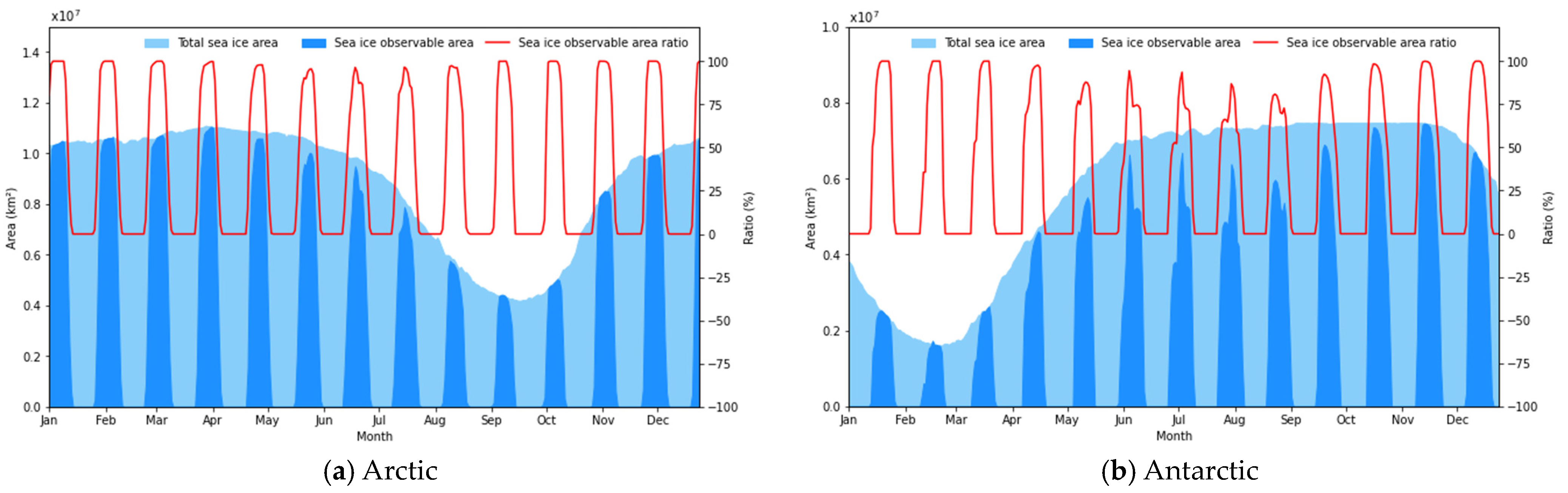
3.3. Potential Applications in Sea Ice Monitoring

As an important component of the polar cryosphere, sea ice significantly responds to polar weather and global climate change. This section conducts simulated calculations and analysis of the coverage and characteristics of MH-BiSAR on sea ice to evaluate its observational potential. The daily polar sea ice data for the entire year of 2023 released by the National Snow and Ice Data Center (NSIDC) are considered as the actual sea ice area values [31], and the daily coverage of sea ice at the North and South Poles by MH-BiSAR for that year was simulated and calculated. The results are shown in Figure 15.

It can be observed that for most months of the year, MH-BiSAR achieves a daily revisit coverage of over 95% for several days to about half a month with respect to Arctic sea ice. However, for Antarctic sea ice, there is a noticeable decrease during the winter months (May to September). This is primarily due to the presence of the Antarctic continent, resulting in an increased proportion of sea ice area in the low-latitude regions of Antarctica, which is more pronounced due to the longitude selection characteristics of MH-BiSAR in this region. Nonetheless, even under these conditions, it still achieves a daily revisit coverage of over 80% for multiple days each month, demonstrating good coverage performance. Furthermore, during the summer melting period of sea ice in the Arctic (March to September) and in the Antarctic (September to March of the following year), there is very good daily revisit coverage within each month. This characteristic provides MH-BiSAR with a significant advantage in observing the summer sea ice melting processes in both the Arctic and Antarctic. Therefore, making use of the large-scale, multi-day continuous observation capabilities of MH-BiSAR for polar sea ice will enable a better capture of its dynamic change information, providing richer data support for a deeper understanding of the freeze-thaw cycle and influencing factors of sea ice.

4. Limitations of Coverage Analysis Based on Observation Geometry

In this paper, the MS-BiSAR observation geometry model is utilized. By integrating the SNR requirements and using the incidence angle as a constraint, the geometric coverage capability of MH-BiSAR for ground observation is calculated and analyzed. This study facilitates a preliminary exploration of the MH-BiSAR’s potential applications for Earth observation in polar regions. However, it should be noted that given the complexity of the SAR imaging mechanism, the accurate effective observation coverage that the MH-BiSAR can achieve still requires further comprehensive consideration of the following factors.

4.1. Spatial Resolution

Spatial resolution is one of the most important performance indicators for SAR. Unlike monostatic SAR, the transmitting and receiving antennas of BiSAR are separately mounted on platforms that are in different positions and states of motion. In such configurations, the gradient angle of iso-range and iso-Doppler are typically non-orthogonal. Under these circumstances, the spatial resolution of the BiSAR can be quantitatively described by three parameters: the range resolution ${\rho }_{gr}$, the azimuth resolution ${\rho }_{ga}$, and the resolution direction angle ${\alpha }_D$. Figure 16 illustrates the ground resolution cell of BiSAR.

The area of the resolution cell for BiSAR can be expressed as:

$$\Delta S=\frac{{\rho }_{gr}{\rho }_{ga}}{\left|\sin {\alpha }_D\right|}$$

(3)

As indicated by the equation, unlike monostatic SAR, the area of the resolution cell for BiSAR is related not only to the values of ${\rho }_{gr}$ and ${\rho }_{ga}$, but also to the ${\alpha }_D$. As ${\alpha }_D$ approaches 90°, the resolution cell area is minimized, enabling high-resolution two-dimensional ground imaging. However, any deviation of ${\alpha }_D$ from 90° increases the resolution of the cell area, thus reducing imaging resolution. Meanwhile, since the resolution cell is no longer rectangular, it causes significant geometric distortion in the remote sensing imagery, which complicates the interpretation of these images.

The two-dimensional resolution of SAR images is determined from the resolution capabilities in range and Doppler frequency. Figure 17 shows the iso-range and iso-Doppler contours of the L-band MH-BiSAR in the Arctic region at different times.

To achieve better range resolution, denser iso-range lines are required. The ground range resolution is determined by the transmitted bandwidth $B_r$, the bistatic angle $\beta$, and the equivalent bistatic incidence angle $\Phi$, with the expression as follows:

$${\rho }_{gr}=\frac{k_{1}c}{2B_r\cos \frac{\beta }{2}\sin \Phi }$$

(4)

where $c$ is the constant speed of light, and $k_1$ is a constant related to the transmitted signal waveform. When the transmitted signal is a rectangular pulse, $k_1=0.886$.

To achieve a 7.5-m slant range resolution, a signal bandwidth of 20 MHz is required, which is feasible for a Moon-based radar with a fixed station. When the $\Phi$ is 60°, a ground range resolution on the order of ten meters can be achieved under small bistatic angles, allowing for the observation of targets such as sea ice. However, as the bistatic angle increases, the range resolution will significantly decrease, posing challenges for effective target observation coverage.

Simultaneously, achieving better azimuth resolution requires a larger Doppler bandwidth within the synthetic aperture time ($T_a$). The ground azimuth resolution can be determined based on radar parameters and platform motion parameters, as given by:

$${\rho }_{ga}=\frac{k_2\lambda }{T_a{\omega }_E}$$

(5)

where $k_2$ is a constant depending on the azimuth profile, λ is the wavelength of the transmitted signal, and ${\omega }_E$ is the equivalent bistatic angular speed. Given that the orbital altitude of the Moon and the apogee of HEO satellites are significantly higher than that of LEO satellites, in this case, their angular speed around Earth is considerably lower during the imaging process in ECEF.

Considering that HEO satellites have very low speeds near apogee (as low as 20 m/s), at this time, the Doppler shift of the target’s echo is primarily due to the relative velocity between the Moon and the target. In order to achieve sufficient azimuth resolution to meet observational requirements, MH-BiSAR requires longer synthetic aperture times. In the L-band, to achieve azimuth resolutions on the order of 10 m, synthetic aperture times of several hundred seconds are needed. This poses challenges in imaging time-varying scatterers such as vegetation and sea surfaces. These factors should also be comprehensively considered in assessing the effective coverage of MH-BiSAR.

Figure 18 illustrates the angles between the gradients of iso-range and iso-Doppler (${\alpha }_D$) at the corresponding times presented in Figure 17, with various colors indicating distinct angle values.

It can be seen that at different times, the angles between the iso-range and iso-Doppler gradient of the same area on the Earth’s surface varies greatly. In this context, gray denotes areas where, despite being geometrically observable, the gradient angles are either less than 60 degrees or greater than 120 degrees. As previously mentioned, conditions like these are likely to result in significant geometric distortions within the targeted area. Therefore, it is necessary to determine the threshold for deviation from 90 degrees for this value based on the specific requirements of the application.

Due to the variation in the distribution of iso-range and iso-Doppler contours on the ground at different bistatic configurations and times, it is necessary to set appropriate receiving satellite orbits and observation times for different areas in order to determine and improve the spatial resolution of MH-BiSAR, thus obtaining better coverage characteristics.

4.2. Radiometric Resolution

Radiometric resolution is a parameter closely related to image quality. With the same number of looks, its performance is primarily determined by the imaging SNR. For BiSAR, the imaging SNR after range compression and azimuthal coherent integration can be expressed as:

$$\mathrm{S}\mathrm{N}\mathrm{R}=\frac{P_{ave}{G}_T{G}_R{\sigma }_0{\rho }_{ga}{\rho }_{gr}{\lambda }^2{T}_a}{{\left(4\pi \right)}^3{R}_T^2{R}_R^2{L}_{T}k{T}_R{F}_n}$$

(6)

where $P_{ave}$ represents the average transmit power of the transmitter, $G_T$ and $G_R$ are the antenna gain of the transmitter and the receiver, respectively, ${\sigma }_0$ is the normalized bistatic scattering coefficient of the target, $R_t$ and $R_R$ are the slant ranges from the transmitter and receiver to the observation target, respectively, $L_T$ represents the propagation loss, and $k$, $T_R$, $F_n$ are the Boltzmann constant, the receiver noise temperature, and the receiver noise factor, respectively.

For MH-BiSAR, given the vast expanse of the lunar surface and the ample energy supply from lunar bases, it is feasible to achieve high transmission power and a large antenna aperture for the transmitter. This significantly reduces the requirements for the antenna aperture of the receiver on the satellite platform. Benefiting from the low gravity and vacuum environment on the lunar surface, deploying lightweight large-aperture antennas becomes possible. With an antenna efficiency of 0.8, by deploying parabolic antennas with apertures of 80 m and 160 m, the required transmission power of the Moon-based transmitter to achieve the same ground power density as a typical satellite-based illuminator [32] is shown in

Table 3. Required transmit power for a Moon-based transmitter to achieve ground power density comparable to typical spaceborne illuminators.

Illuminator	Band	Power Density (dbW·m−2)	Required Transmit Power (kW)
			160 m	80 m
LEO-SAR	C	−50.3	256.3	1044.2
MEO-SAR	C	−64.5	9.7	39.7
GEO-SAR	L	−74.3	19.0	77.4

.

The table shows that to achieve comparable ground power density with spaceborne illuminators at different orbital altitudes and in different operational bands, the required transmission power for a Moon-based transmitter varies significantly in magnitude. Meanwhile, increasing the antenna aperture of the Moon-based transmitter significantly reduces the required transmission power. To achieve ground power density equivalent to that of GEO and MEO SAR, the required transmission power for a Moon-based transmitter is only in the range of tens to several tens of kilowatts. This is feasible for Moon-based radars with fixed stations and ample energy supply. However, it is also noted that to achieve ground power density equivalent to that of LEO SAR, the required transmission power increases significantly in magnitude. Therefore, when forming a BiSAR with the aforementioned platforms, suitable imaging modes need to be considered to extend the synthetic aperture time and thereby improve the imaging SNR.

In addition to the parameters of the radar system, the SNR is also closely linked to the bistatic scattering characteristics of ground targets. The normalized bistatic scattering coefficients of a random rough surface are calculated at the L-band using the advanced integral equation model (AIEM) [33]. The model’s input includes correlation length ($l$), surface-root-mean square height ($s$), dielectric constant ($\epsilon$), polarization mode, wave number ($k$) and observation geometric angles. The simulation results are presented in Figure 19.

Figure 19 depicts the variation of the normalized bistatic scattering coefficient of Gaussian random rough surfaces with changes in the observation geometry configuration under a set of electromagnetic scattering parameters. It can be observed that with the change of observation geometry, the normalized bistatic scattering coefficients of the target vary significantly. Furthermore, the target’s electromagnetic scattering characteristics will vary across different polarization modes. This will provide more information for ground parameter inversion. However, it may also result in the SNR being unable to meet imaging requirements under certain observation geometries.

Due to the reasons mentioned above, when designing radar parameters and receiving satellite orbits, it is necessary to integrate observation geometry and comprehensively consider the system parameters of the observing radar as well as the bistatic scattering characteristics of the target. This ensures that the radiometric resolution meets application requirements, thereby achieving effective coverage of the observed area.

Meanwhile under certain scattering azimuth angles ($\varphi$), such as forward-scattering imaging, the normalized bistatic scattering coefficient of the target is much higher than that during backward scattering. At this point, MH-BiSAR has the potential for Earth observation with low transmit power.

In addition to the factors previously mentioned, the imaging modes of the radar and the spatiotemporal variations of the ionosphere, among other factors, also affect the effective imaging coverage area of MH-BiSAR. This implies that the coverage characteristics obtained solely from observation geometry have their limitations. Therefore, based on the preliminary research presented in this paper, a comprehensive evaluation of the ground observation coverage by MH-BiSAR still requires further consideration of multiple factors.

5. Discussion

In this paper, a preliminary study was conducted through observation geometry simulation to investigate the coverage characteristics of MH-BiSAR in polar regions. The simulation results indicate that MH-BiSAR can achieve large-scale, high revisit rate observation capabilities of the Earth’s polar regions within each sidereal month. This capability allows for the provision of temporally consistent and spatially continuous polar observation data, presenting significant advantages in observing large-scale polar scientific phenomena compared to current LEO SAR systems.

Through simulation calculations, it was found that MH-BiSAR exhibits variations in coverage for different latitudes and longitudes within polar regions. In higher latitude regions, such as those near the poles, daily revisit can be achieved twice a day with longer cumulative daily coverage time, but there are fewer observable days compared to lower latitudes. Conversely, in relatively lower latitude regions, more days (at least 8 days) of daily revisit observations can be achieved, albeit with shorter daily cumulative observation times.

Additionally, MH-BiSAR’s daily observable time varies with longitude, particularly noticeably in low-latitude polar regions. Therefore, designing satellite orbital parameters based on observational requirements is crucial for improving observation coverage in low-latitude polar regions.

Furthermore, it was noted that MH-BiSAR’s observational performance exhibits periodic variations over an 18.6-year lunar nodal period, with the greatest impact occurring near the poles. Lastly, MH-BiSAR demonstrates significant observational coverage advantages for polar sea ice monitoring tasks, potentially enhancing our understanding of phenomena such as summer sea ice melting processes.

It should be noted that, as mentioned earlier, this study is a preliminary exploration based on observational geometry simulation, and there are some issues that need further investigation in future studies.

Firstly, although previous studies have widely applied simulation of observation coverage based on incidence angle constraints, such methods are limited to qualitative analysis, and the setting of the incidence angle threshold has a considerable impact on the results. Therefore, in future evaluations of observation coverage performance, it is necessary to comprehensively consider important imaging performance indicators for BiSAR, such as spatial and radiometric resolution.

Secondly, this study selected one of the most used HEOs, the Molniya orbit, and discussed the MH-BiSAR configuration based on this orbit. Although the Molniya orbit is widely representative, in recent years, many HEOs have been proposed, potentially enhancing the overall or local coverage capabilities of MH-BiSAR for observations in polar regions.

At the same time, optimization methods for HEO specific to MH-BiSAR should also be further explored. To achieve more comprehensive polar coverage, a possible solution is to deploy a two-satellite system on the Molniya orbit to achieve better coverage. At the same time, a BiSAR imaging scheme based on terrain forward scattering, although it results in a reduction in imaging resolution, can significantly enhance the SNR of the echoes. This approach provides a potential method for expanding coverage regions.

Finally, despite the ephemeris, EOP, and orbit propagators used in this study being widely recognized in the relevant field, there may still be some approximation errors introduced during the simulation process, which need to be further discussed.

6. Conclusions

To address the challenge of achieving both temporal consistency and spatial continuity in Earth observation data of polar regions, this paper proposes an innovative concept of MH-BiSAR, with transmitters on the Moon and receivers on HEO satellites. Compared to the existing LEO SAR, it offers a significantly improved observation scale and a shorter continuous revisit period. At the same time, it also overcomes various engineering challenges associated with HEO SAR, achieving lower costs and longer lifespans.

Although there are currently technical challenges in deploying SAR observation stations on the Moon, these challenges are expected to be overcome as lunar infrastructure continues to improve. MH-BiSAR will provide new perspectives for the study of large-scale scientific phenomena and make significant contributions to the advancement of polar research.

References

1. Torres, R.; Snoeij, P.; Geudtner, D.; Bibby, D.; Davidson, M.; Attema, E.; Potin, P.; Rommen, B.; Floury, N.; Brown, M.; et al. GMES Sentinel-1 mission. Remote Sens. Environ. 2012, 120, 9–24. [Google Scholar] [CrossRef]
2. Pan, L.; Powell, E.M.; Latychev, K.; Mitrovica, J.X.; Creveling, J.R.; Gomez, N.; Hoggard, M.J.; Clark, P.U. Rapid postglacial rebound amplifies global sea level rise following West Antarctic Ice Sheet collapse. Sci. Adv. 2021, 7, eabf7787. [Google Scholar] [CrossRef] [PubMed]
3. Rounce, D.R.; Hock, R.; Maussion, F.; Hugonnet, R.; Kochtitzky, W.; Huss, M.; Berthier, E.; Brinkerhoff, D.; Compagno, L.; Copland, L.; et al. Global glacier change in the 21st century: Every increase in temperature matters. Science 2023, 379, 78–83. [Google Scholar] [CrossRef]
4. Hwang, B.; Aksenov, Y.; Blockley, E.; Tsamados, M.; Brown, T.; Landy, J.; Stevens, D.; Wilkinson, J. Impacts of climate change on Arctic sea ice. MCCIP Sci. Rev. 2020, 2020, 208–227. [Google Scholar]
5. Trishchenko, A.P.; Garand, L. Observing polar regions from space: Advantages of a satellite system on a highly elliptical orbit versus a constellation of low Earth polar orbiters. Can. J. Remote Sens. 2012, 38, 12–24. [Google Scholar] [CrossRef]
6. Asmus, V.V.; Milekhin, O.E.; Kramareva, L.S.; Khailov, M.N.; Shirshakov, A.E.; Shumakov, I.A. Arktika-M: The World’s First Highly Elliptical Orbit Hydrometeorological Space System. Russ. Meteorol. Hydrol. 2021, 46, 805–816. [Google Scholar] [CrossRef]
7. Li, C.; Liu, J.; Duan, C. Imaging characteristic for large elliptical orbit SAR. In Proceedings of the 2019 6th Asia-Pacific Conference on Synthetic Aperture Radar (APSAR), Xiamen, China, 26–29 November 2019; pp. 1–5. [Google Scholar]
8. Hu, X.; Wang, P.; Zeng, H.; Guo, Y. An Improved Equivalent Squint Range Model and Imaging Approach for Sliding Spotlight SAR Based on Highly Elliptical Orbit. Remote Sens. 2021, 13, 4883. [Google Scholar] [CrossRef]
9. Hobbs, S.; Mitchell, C.; Forte, B.; Holley, R.; Snapir, B.; Whittaker, P. System Design for Geosynchronous Synthetic Aperture Radar Missions. IEEE Trans. Geosci. Remote Sens. 2014, 52, 7750–7763. [Google Scholar] [CrossRef]
10. Moussessian, A.; Chen, C.; Edelstein, W.; Madsen, S.; Rosen, P. System concepts and technologies for high orbit SAR. In Proceedings of the IEEE MTT-S International Microwave Symposium Digest, 2005, Long Beach, CA, USA, 17 June; 2005; pp. 1623–1626. [Google Scholar]
11. Lu, Y.F.; Shao, Q.; Yue, H.H.; Yang, F. A Review of the Space Environment Effects on Spacecraft in Different Orbits. IEEE Access 2019, 7, 93473–93488. [Google Scholar] [CrossRef]
12. Trichtchenko, L.D.; Nikitina, L.V.; Trishchenko, A.P.; Garand, L. Highly Elliptical Orbits for Arctic observations: Assessment of ionizing radiation. Adv. Space Res. 2014, 54, 2398–2414. [Google Scholar] [CrossRef]
13. Xu, L.; Li, H.; Pei, Z.; Zou, Y.; Wang, C. A Brief Introduction to the International Lunar Research Station Program and the Interstellar Express Mission. Chin. J. Space Sci. 2022, 42, 511–513. [Google Scholar] [CrossRef]
14. Weiren, W. International Lunar Research Station. Aerosp. China 2023, 24, 10–14. [Google Scholar]
15. Guo, H.D.; Ding, Y.X.; Liu, G. Moon-based Earth observation. Sci. Bull. 2022, 67, 2036–2039. [Google Scholar] [CrossRef]
16. Guo, H.D.; Liu, G.; Ding, Y.X. Moon-based Earth observation: Scientific concept and potential applications. Int. J. Digit. Earth 2018, 11, 546–557. [Google Scholar] [CrossRef]
17. Fornaro, G.; Franceschetti, G.; Lombardini, F.; Mori, A.; Calamia, M. Potentials and Limitations of Moon-Borne SAR Imaging. IEEE Trans. Geosci. Remote Sens. 2010, 48, 3009–3019. [Google Scholar] [CrossRef]
18. Liu, H.Y.; Guo, H.D.; Liu, G.; Ding, Y.X. An exploratory study on moon-based observation coverage of sea ice from the geometry. Int. J. Remote Sens. 2020, 41, 6089–6098. [Google Scholar] [CrossRef]
19. Behner, F.; Reuter, S.; Nies, H.; Loffeld, O. Synchronization and Processing in the HITCHHIKER Bistatic SAR Experiment. IEEE J. Sel. Top. Appl. Earth Obs. Remote Sens. 2016, 9, 1028–1035. [Google Scholar] [CrossRef]
20. Cai, Y.H.; Li, J.F.; Yang, Q.Y.; Liang, D.; Liu, K.Y.; Zhang, H.; Lu, P.P.; Wang, R. First Demonstration of RFI Mitigation in the Phase Synchronization of LT-1 Bistatic SAR. IEEE Trans. Geosci. Remote Sens. 2023, 61, 5217319. [Google Scholar] [CrossRef]
21. Sun, Z.C.; Wu, J.J.; Huang, Y.L.; Yang, J.Y.; Yang, H.G.; Yang, X.B. Performance Analysis and Mission Design for Inclined Geosynchronous Spaceborne-Airborne Bistatic SAR. In Proceedings of the 2015 IEEE Radar Conference (RadarCon), Arlington, VA, USA, 10–15 May 2015; pp. 1177–1181. [Google Scholar]
22. Sun, Z.C.; Wu, J.J.; Pei, J.F.; Li, Z.Y.; Huang, Y.L.; Yang, J.Y. Inclined Geosynchronous Spaceborne-Airborne Bistatic SAR: Performance Analysis and Mission Design. IEEE Trans. Geosci. Remote Sens. 2016, 54, 343–357. [Google Scholar] [CrossRef]
23. Zhang, K.; Guo, H.; Jiang, D.; Han, C. Analysis of Geometric Characteristics and Coverage for Moon-Based/Spaceborne Bistatic SAR Earth Observation. Remote Sens. 2023, 15, 2151. [Google Scholar] [CrossRef]
24. Folkner, W.M.; Williams, J.G.; Boggs, D.H.; Park, R.S.; Kuchynka, P. The planetary and lunar ephemerides DE430 and DE431. Interplanet. Netw. Prog. Rep. 2014, 196, 42–196. [Google Scholar]
25. Bizouard, C.; Lambert, S.; Gattano, C.; Becker, O.; Richard, J.-Y. The IERS EOP 14C04 solution for Earth orientation parameters consistent with ITRF 2014. J. Geod. 2019, 93, 621–633. [Google Scholar] [CrossRef]
26. Xu, Z.; Chen, K.S.; Liu, G.; Guo, H.D. Spatiotemporal Coverage of a Moon-Based Synthetic Aperture Radar: Theoretical Analyses and Numerical Simulations. IEEE Trans. Geosci. Remote Sens. 2020, 58, 8735–8750. [Google Scholar] [CrossRef]
27. Kidder, S.Q.; Vonderhaar, T.H. On the Use of Satellites in Molniya Orbits for Meteorological Observation of Middle and High-Latitudes. J. Atmos. Ocean. Technol. 1990, 7, 517–522. [Google Scholar] [CrossRef]
28. Bonin, G.; King, J.; Brett, M.; Wilson, S. Antarctic Broadband: Ka-Band Communications for the Bottom of the Earth. In Proceedings of the 30th AIAA International Communications Satellite System Conference (ICSSC), Ottawa, ON, Canada, 24–27 September 2012; p. 15191. [Google Scholar]
29. Moccia, A.; Renga, A. Synthetic Aperture Radar for Earth Observation from a Lunar Base: Performance and Potential Applications. IEEE Trans. Aerosp. Electron. Syst. 2010, 46, 1034–1051. [Google Scholar] [CrossRef]
30. Trishchenko, A.P.; Garand, L. Spatial and Temporal Sampling of Polar Regions from Two-Satellite System on Molniya Orbit. J. Atmos. Ocean. Technol. 2011, 28, 977–992. [Google Scholar] [CrossRef]
31. Fetterer, F.; Knowles, K.; Meier, W.N.; Savoie, M.; Windnagel, A.K. Sea Ice Index; Version 3; Data Set; National Snow and Ice Data Center: Boulder, CO, USA, 2017. [Google Scholar] [CrossRef]
32. Wu, J.; Sun, Z.; Yang, J.; Lyu, Z.; Li, D.; Miao, Y.; Chen, T.; Zuo, W.; Li, C.; Hai, Y.; et al. Spaceborne Airborne Bistatic SAR Using GF-3 Illumination—Technology and Experiment. Radar Science and Technology. Radar Sci. Technol. 2021, 19, 241–247. [Google Scholar]
33. Wu, T.D.; Chen, K.S.; Shi, J.C.; Lee, H.W.; Fung, A.K. A study of an AIEM model for bistatic scattering from randomly rough surfaces. IEEE Trans. Geosci. Remote Sens. 2008, 46, 2584–2598. [Google Scholar] [CrossRef]
Figure 1. A conceptual illustration of MH-BiSAR for Earth’s polar regions observation.
Remotesensing 16 02086 g001
Figure 2. Tracks of sublunar points over a week.
Remotesensing 16 02086 g002
Figure 3. Latitudes and Longitudes of sublunar points over one orbital period.
Remotesensing 16 02086 g003
Figure 4. Latitudes of annual northernmost and southernmost sublunar points from 1983–2023.
Remotesensing 16 02086 g004
Figure 5. Graphic layout for elliptical orbit and definition of Keplerian orbital elements.
Remotesensing 16 02086 g005
Figure 6. A Molniya orbit is viewed perpendicular to the plane of the orbit. Dots are placed each hour. The labels are hours from apogee.
Remotesensing 16 02086 g006
Figure 7. Nadir track of satellites in Molniya orbit (blue) and inverted Molniya orbit (red). Dots are placed each 10 min.
Remotesensing 16 02086 g007
Figure 8. Simplified MS-BiSAR Earth observation geometric model. O m b o is the Moon-based observatory, O m is the selenocenter, O E is the geocenter, and O s is the satellite. θ i m and θ i s are the threshold for the incidence angle of the transmitter and receiver, respectively. S 1 and S 2 are the boundaries of the observable region of the satellite receiver. Meanwhile, M 1 and M 2 are the boundaries of the observable region of the Moon-based observatory. The red region is defined as the observable region of MS-BiSAR (not to scale for the sake of clarity).
Remotesensing 16 02086 g008
Figure 9. Observable spans of the Moon-based platform for Arctic sampling points over one orbital period.
Remotesensing 16 02086 g009
Figure 10. Observable spans of the Molniya orbit platform for Arctic sampling points over one lunar orbital period.
Remotesensing 16 02086 g010
Figure 11. Nadir track of satellites in the two-satellite system on Molniya Orbit. Different colors represent the individual tracks of the two satellites. Dots are placed each 10 min.
Remotesensing 16 02086 g011
Figure 12. Observable spans of the satellites in the two-satellite system on Molniya Orbit for Arctic sampling points over one lunar orbital period.
Remotesensing 16 02086 g012
Figure 13. Observable spans of MH-BiSAR for Arctic sampling points over one orbital period.
Remotesensing 16 02086 g013
Figure 14. Daily cumulative observable time of MH-BiSAR for the polar regions from 1 to 28 January 2023.
Remotesensing 16 02086 g014aRemotesensing 16 02086 g014b
Figure 15. Coverage of sea ice in polar regions by MH-BiSAR over 2023. The deep blue area represents the daily total sea ice area within the polar circle, while the light blue area depicts the daily observable sea ice area values by MH-BiSAR. The red line indicates the ratio of the observable sea ice area to the total sea ice area, representing the extent of sea ice coverage.
Remotesensing 16 02086 g015
Figure 16. The ground resolution cell of BiSAR.
Remotesensing 16 02086 g016
Figure 17. Iso-range and iso-Doppler contours at different times.
Remotesensing 16 02086 g017
Figure 18. Gradient angles of iso-range and iso-Doppler at different times.
Remotesensing 16 02086 g018
Figure 19. The normalized bistatic scattering coefficients with respect to observation geometry ( k l = 6.3 , k s = 0.63 , ε = 5 , θ m = 65 ° ).
Remotesensing 16 02086 g019