X-Band Radar Detection of Small Garbage Islands in Different Sea State Conditions

Abstract

This paper presents an assessment of X-band radar’s detection capability to monitor Small Garbage Islands (SGIs), i.e., floating aggregations of marine litter consisting chiefly of plastic, under changing sea states. For this purpose, two radar measurement campaigns were carried out with controlled releases at sea of SGI modules assembled in the laboratory. One campaign was carried out with a calm sea and almost no wind in order to determine the X-band radar system’s detection capabilities in an ideal scenario, while the other campaign took place with rough seas and wind. An analysis of the data acquired during the campaigns confirmed that X-band radar can detect small aggregations of litter floating on the sea surface. To demonstrate the radar’s ability to detect SGIs, a statistical analysis was carried out to calculate the probability of false alarm and the probability of detection for two releases at two different distances from the radar. For greater readability of this work, all of the results obtained are presented both in terms of radar intensity and in terms of the radar cross-section relating to both the targets and the clutter. Another interesting study that is presented in this article concerns the measurement of the speed of movement (drift) of the SGIs compared with the measurement of the speed of the surface currents provided at the same time by the radar. The study also identified the radar detection limits depending on the sea state and the target distance from the antenna.

1. Introduction

Though undoubtedly useful in many ways, plastic has become one of today’s major environmental problems due to poor management of its life cycle [1]. Of the annual global production of plastic, estimated at around 320 million metric tons, a significant amount has an ephemeral use and quickly turns into waste. A small portion is recycled or incinerated, while the majority ends its life cycle in landfills or natural environments, including the oceans [2].

Due to its abundance, plastic accounts for about 75% of marine litter [3,4,5]. Moreover, since it is transported much more quickly than it degrades, plastic can travel very far after it is discarded [5,6,7,8]. As a result, every ocean on the globe has been contaminated by plastic. The problem has reached the point where marine plastic pollution can be considered irreversible and globally ubiquitous [9].

Plastic’s steady accumulation in the oceans is a source of great concern due to its persistence over time and harmful effects on ocean health, which directly impact marine habitats, wildlife, food safety, human health, coastal tourism and climate regulation [10,11,12].

The seriousness of the situation has prompted the world scientific community to pursue a twofold goal: investigating the impact of plastic on marine habitats and organisms and monitoring the presence and movement of plastic litter in the oceans and along their coasts. For a review of different types of marine litter and plastic monitoring, readers are referred to [13,14,15,16,17,18,19].

Identifying and tracking plastic litter is essential in order to optimize pollution containment measures and monitor their effectiveness over time and space. In situ monitoring techniques can yield very valuable information on the presence of plastic in the oceans. However, such techniques are not always cost-effective or practically feasible because of the vastness of the oceans and coastal regions, the temporal dynamics of plastic inflows and plastic waste containment and management policies [20].

In order to overcome the intrinsic limitations of in situ techniques, a growing number of researchers are exploring the potential of remote sensing to monitor plastics in the oceans.

In recent years, the number of studies based on remote sensing techniques for monitoring beaches [21,22] and floating litter on the sea surface [23,24] has steadily increased. Although remote sensing techniques have considerable potential for long-term global-scale monitoring of marine plastic pollution, studies investigating the remote sensing of marine plastic litter are still under development [25,26,27,28,29,30,31]. From a methodological standpoint, Ref. [31] discusses the following remote sensing platforms for monitoring marine plastic litter:

• Airborne platforms for the remote detection of plastic litter in coastal and marine environments. For further information, see [30,31,32,33,34,35,36,37].
• Spaceborne platforms for the remote detection of marine plastic litter. For further information, see [28,34,38,39,40,41,42,43].
• Underwater platforms for monitoring subsurface and submerged marine plastic debris. For further information, see [44,45,46,47,48].
• LiDAR, radar and sonar remote sensing for marine debris monitoring. For further information, see [23,28,45,49,50,51,52,53,54,55].

This paper builds on the findings illustrated in [51], where analyzing the intensity of the radar signal backscattered by targets floating on the sea surface enabled us to demonstrate that, in calm sea conditions with almost no wind, X-band radars can identify and characterize accumulations of plastic debris. Though X-band radars were initially conceived as navigation support tools, their ability to detect targets at sea has given them an important role in remote sea state monitoring, the reconstruction of surface current fields and bathymetry [56,57,58,59].

Specifically, the investigation presented here analyzed backscatter intensity from floating targets released in two measurement campaigns in order to identify the limits of X-band radar detection capability with a rising sea state, in windy conditions and as a function of the distance between the target and radar antenna.

It is important to underline that X-band radar systems have a particular acquisition geometry, called the grazing angle [60], where the transmitted pulse is almost parallel to the sea surface. Under this condition, the backscattered signal from the targets is very low, and this makes the analysis very challenging, particularly for low-intensity objects like those analyzed in this work.

The second campaign also employed a technique for processing radar data over time, exploiting the time correlation of the targets to maximize the radar detection capability in the presence of clutter. The results demonstrate that the radar can be used to detect and track small floating plastic islands in the presence of clutter up to a distance of 0.27 NM from the radar and up to sea state 4 on the Beaufort scale.

2. Materials and Methods

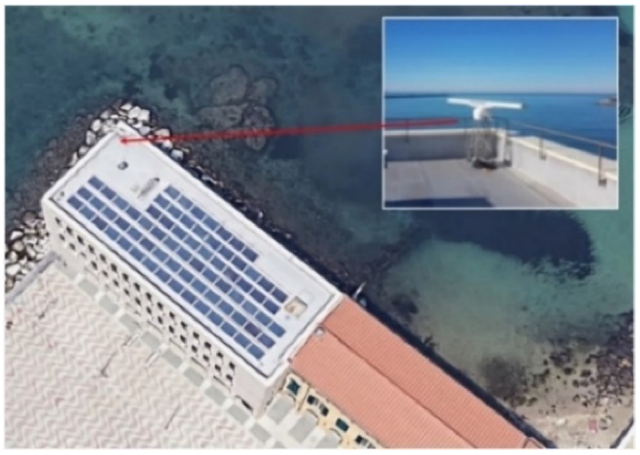
2.1. X-Band Radar Specification

A 25 kW Consilium/Selesmar SRT X-band (9.3 Ghz) radar system with an antenna length of 9 feet was used for the measurement campaigns. The radar, owned by the National Research Council (CNR) and purchased with funds from the RITMARE project, is installed on the roof of the Scoglio della Regina building in Livorno at the coordinates Lat: 43_32021.1000N and Lon: 10_17058.9000E (Figure 1).

Table 1. The operating parameters of the radar system.

Radar Parameter	Value
Peak power	25 kW
Antenna length	2.7 m
Radar scale	0.98 NM
Antenna rotation period (Δt)	2.4 s
Spatial image spacing (Δx and Δy)	3.5 m
Cross-range resolution	~9 m
Azimuth resolution	~1°
Antenna height	~10 m
View angular sector	360°N
Radar’s per-frame coherent integration time	48 s

summarizes the operating parameters of the radar system used for the measurement campaigns.

2.2. Description of the Survey Area

The measurement campaigns were carried out in the stretch of sea located immediately south of the main entrance to the Livorno harbor. This stretch of sea has a radius of approximately 0.86 nautical miles and features persistently intense maritime traffic and numerous signals (beacons, lighthouses, buoys, etc.) warning of navigation hazards. Figure 2 shows an aerial view of the survey area overlaid with the corresponding radar image on a color scale (from blue to red) as a function of the intensity of the radar signal received from the targets normalized with respect to the maximum value. In particular, blue is associated with low intensity, and red with high intensity.

2.3. Small Garbage Island (SGI) Module Construction

Before starting the radar measurement campaigns, four SGI modules were constructed in the laboratory in order to ensure that measurements would be repeatable and standardizable. The module characteristics are summarized below:

• T0: a target measuring 1 m × 1 m made up of litter of various kinds (plastic, wood, metal, fishing nets, etc.), which approximates small aggregations of floating litter.
• T1: a 1 m × 1 m target consisting mainly of plastic litter.
• T2: a module consisting of three plastic bottles bundled together with a zip tie.
• T3: a module consisting of a single plastic bottle.

Figure 3 shows the T0 and T1 targets used during the measurement campaigns. For further information on the construction of the targets, readers are referred to [51].

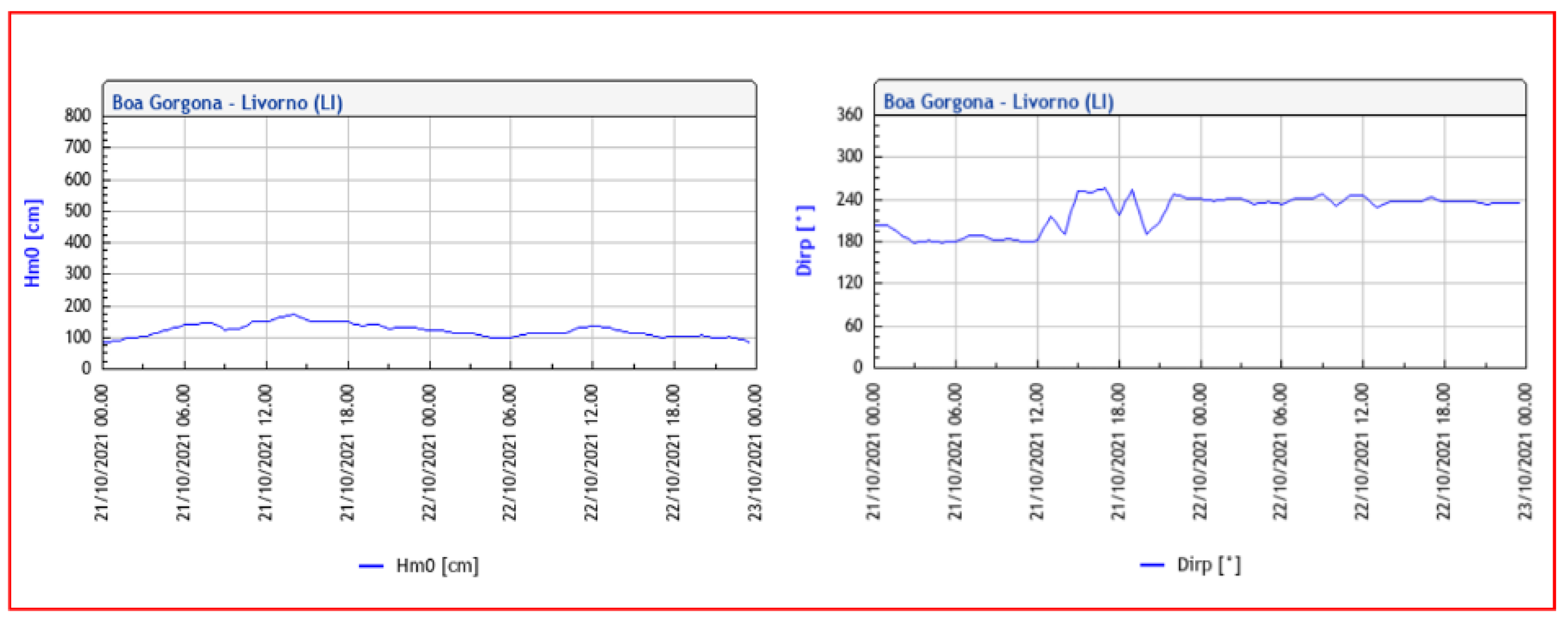
2.4. Measurement Campaigns

Two separate measurement campaigns were conducted: the first (31 July 2020), with a calm sea and almost no wind, gauged the radar’s sensitivity under ideal conditions; the second (21 October 2021), with wind and rough seas, identified the upper clutter limit at which X-band nautical radar can detect SGIs.

Figure 4 shows the characteristic sea state parameters measured by the wave radar during the second campaign (13:13 UTC) on the left and the associated directional spectrum on the right.

Figure 5 shows plots of the average wave height and direction of the waves recorded by the Tuscany regional meteorological center’s Gorgona wave buoy from midnight on 21 October 2021 (the date of the second survey campaign) to midnight on 23 October 2021, which substantially confirm the wave radar measurements. The wave buoy is located about 17 nautical miles from the survey area at the coordinates LAT: 43°34′11.99″N and LON: 9°57′25.21″E.

Figure 6 shows the wind directions and speeds recorded at a height of 10 m during the measurement campaigns by the anemometer installed at the ISPRA (Institute for Environmental Protection and Research) tidal weather station. As the anemometer is located about one kilometer from the test area (at coordinates LAT: 43°32′46″N and LON: 10°17′58″E), the readings can be considered representative of the conditions on the sea during data collection.

To evaluate radar detection capabilities and identify the range limits in which targets can be identified, SGIs were released at three different distances from the antenna during the first measurement campaign:

• First release: 0.12 nautical miles.
• Second release: 0.24 nautical miles.
• Third release: 0.39 nautical miles.

In the second measurement campaign, only two separate releases of the T0 and T1 targets were carried out because of the higher sea state. Distances from the antenna were as follows:

• First release: 0.12 nautical miles.
• Second release: 0.27 nautical miles.

2.5. Radar Data Processing

To assess the radar’s ability to identify targets released into the sea during the measurement campaigns, the intensity of the radar signal backscattered by the modules was analyzed. The radar remained in operation for the entire duration of the measurement, collecting raw data that were then analyzed in the laboratory.

In the first measurement campaign, targets were identified through the following step-by-step radar data analysis procedure:

(a)

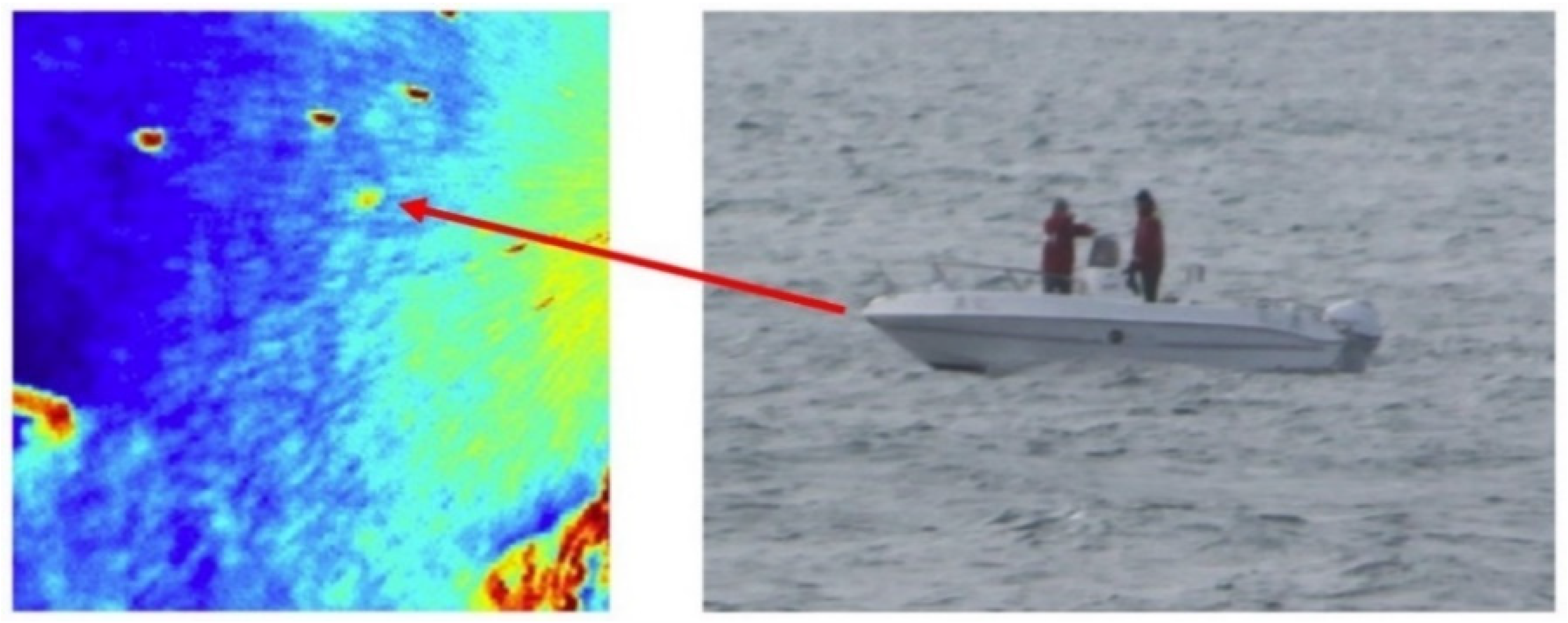
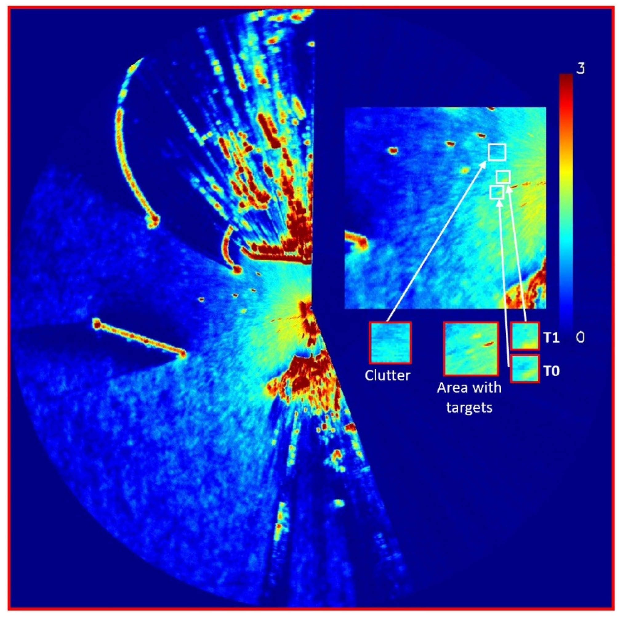
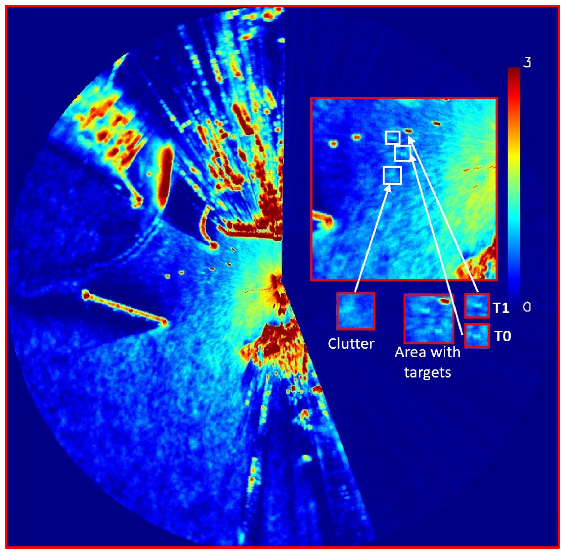
The positions of the SGIs in the radar image were identified from photographs of the survey area. This step is essential, as it provides spatial and temporal references that guarantee that the targets can be precisely identified and co-located.

(b)

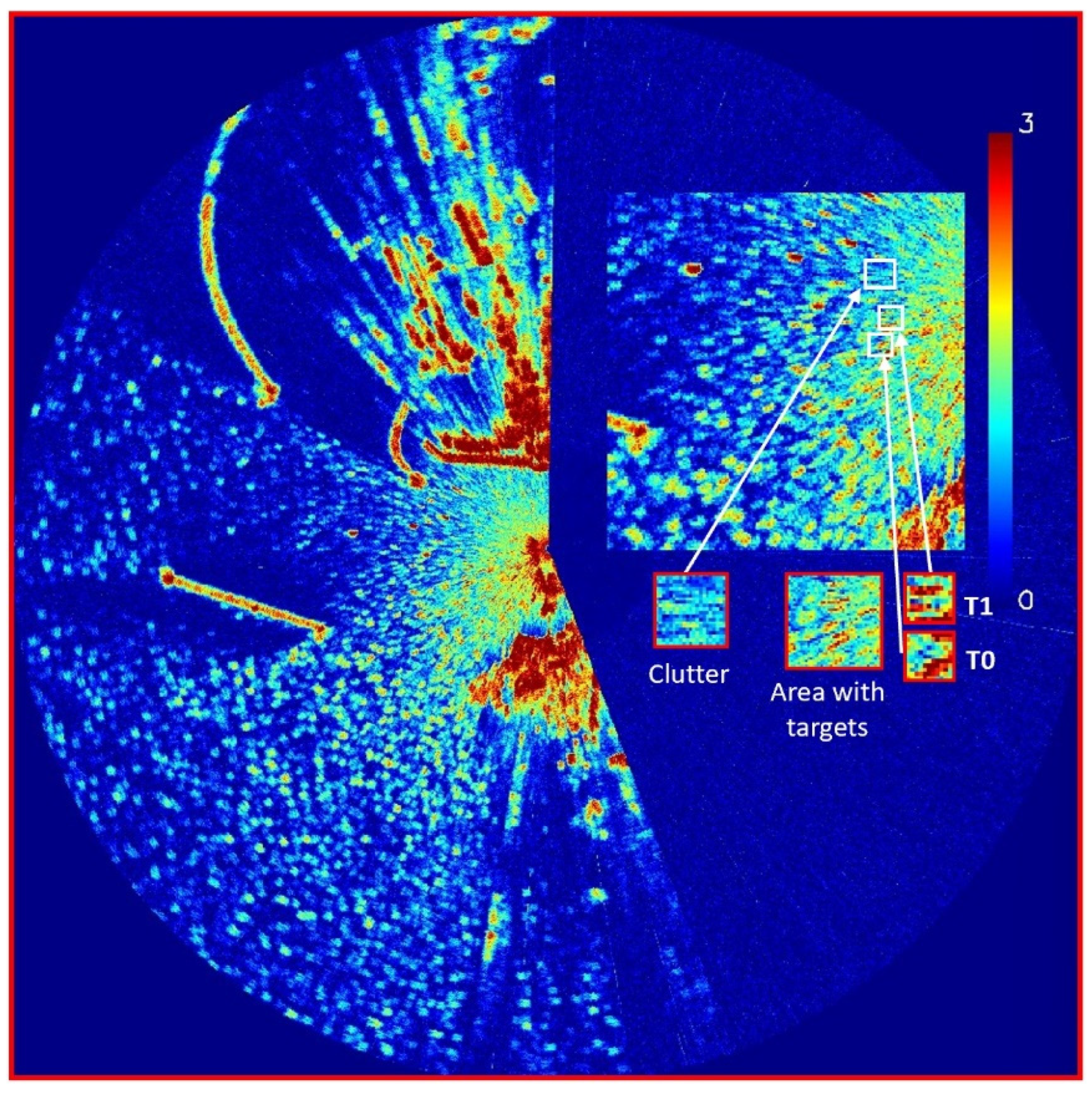
Mobile subareas containing targets T0, T1, T2 and T3 were extracted. As the SGIs tended to drift because of surface currents and wind, these subareas were needed in order to “follow” the targets, taking their speed into account. In the second measurement campaign, the dynamic extraction of the subareas, based on the target’s velocity, was introduced to compensate for the drift of the targets and to have the areolas always perfectly centered on the SGI. This important innovation allowed for overcoming the manual tracing procedure of the subareas used in [51].

(c)

The maximum backscatter intensity detected at each instant of time for each subarea containing targets T0, T1, T2 and T3 was measured.

Further information on radar data analysis is provided in [51].

In the second measurement campaign, the radar signals backscattered by the SGIs were hard to distinguish from the mean sea clutter, as their intensities are comparable in rough seas. This made module identification very difficult. Consequently, in order to overcome the detectability limits of the procedure based on analyzing the intensity of individual radar images, a decluttering procedure was introduced to reduce the clutter. By contrast with the procedure used to process the radar images in the first measurement campaign, step “b” was followed by a further radar image time-averaging step to reduce the fluctuations (the standard deviation) of the instantaneous clutter intensity. The results are detailed in Section 3.

2.6. Representation of Results

In order to facilitate the understanding and application of the results by the scientific community interested in target detection activities, it was decided, for this new paper, to present the results of the second measurement campaign in terms of the Normalized Radar Cross-Section (NRCS) rather than in terms of radar intensity, as was used in the previous work [51]. The use of the NRCS, employing the radar equation and considering specific key parameters of the radar system, aims to make the results comparable among different studies, radar systems, and operational conditions. Below is the procedure used to transform the radar images from intensity to the NRCS representation.

The signal received by a radar decays with a law proportional to the fourth power of the distance, as described by the radar equation:

$$P_r=\frac{P_t{G}^2{\lambda }^{2}RCS}{{\left(4\pi \right)}^3{R}^4}$$

(1)

with the variables defined as follows:

• P_r is the received power.
• P_t is the transmitted power.
• G is the antenna gain.
• λ is the wavelength of the radar signal.
• RCS is the equivalent radar cross-section of the target.
• R is the distance between the radar and the target.

The rapid decay of the signal prevents a clear representation of the image acquired by the radar. To overcome this limitation, all marine radars apply a signal compensation technique aimed at standardizing the radar signal and making it readable and usable for operators. This function is called PRE-STC (Pulse Repetition Interval—Sensitivity Time Control).

The PRE-STC function is typically a non-linear function that increases the amplification of the received signal as a function of time (and thus distance). The goal is to make the intensity of the received radar signal uniform across different distances, improving the ability to detect distant targets.

The specific function used for STC may vary depending on the design of the radar system and the expected operating conditions but often follows an exponential function to effectively compensate for the signal decay with distance. A typical example of an STC function could be an exponential function of the form:

$$A\left(t\right)={A_{0 }e}^{kt}$$

(2)

with the variables defined as follows:

• A(t) represents the amplification applied to the signal at time t.
• A₀ denotes the baseline amplification.
• K is a constant that determines how rapidly the amplification increases over time and varies depending on the radar and operational conditions.
• t represents the time elapsed since the radar pulse emission.

Often, the PRE-STC function alone is not sufficient to properly standardize the radar image. For this reason, many radars apply a second operation known as EXTRA PRE-STC (E-STC). The E-STC function is an additional measure of signal compensation specifically implemented in the radar system to further refine signal management after the application of standard PRE-STC. While PRE-STC is commonly used to compensate for signal decay with distance, E-STC is designed to address specific operational challenges, such as preventing signal saturation or managing an extremely wide dynamic range, which may not be fully addressed by PRE-STC alone.

Without specific details on the E-STC function, it is difficult to provide an accurate description or a general formula, as it may vary significantly depending on the radar system design and specific objectives. E-STC could be a dynamically adjusted function or an algorithm that applies variable compensation based on distance, received signal power, or other signal characteristics to optimize radar image quality.

In our case, lacking access to the specifics of the E-STC function and still wanting to represent the results in terms of the NRCS, we implemented an empirical procedure to simulate the combined use of PRE-STC and E-STC functions. Below is a step-by-step description of the procedure for deriving the NRCS measurement from the radar intensity measurement.

• A target (Tc) with a known RCS is selected from the radar intensity image. As a known target, the vessel used by the authors for the deployment of the SGI is chosen, located 402 m from the radar antenna (see Figure 7). For a target of this type, the literature reports an RCS value approximately equal to 2 m² [61].
• The received power (theoretical) from the radar Equation (1) is estimated for the target Tc:

  $$P_{rTc}=\frac{P_t{G}^2{\lambda }^2{RCS}_{Tc}}{{\left(4\pi \right)}^3{R_{Tc}}^4}$$

  (3)
• The PRE-STC and E-STC functions are empirically constructed to compensate for range decay. For the construction of the function, we tested various solutions and selected the one that best approximates the desired result. In the present case, the choice fell on the following function (P_rpost):

  $$P_{rpost}=k_0{P}_r{R}^4$$

  (4)

  where $k_0$ is a constant depending on the specific radar configuration and has been determined empirically.
• Considering that the radar image we have is a representation in grayscale levels (Im) of the power P_rpost, we determine the factor γ for the known target Tc, which will subsequently be used throughout the radar image:

  $$\gamma =\frac{I_{mTc}}{P_{rpost\_Tc}}$$

  (5)

  with the variables defined as follows:
  • I_mTc is the radar signal intensity of the target Tc expressed in grayscale levels.
  • P_{rpost_Tc} is the post-compensation power of the target Tc.
• At this point, we can obtain the power P_r for the entire radar image by reversing Equation (4):

  $$P_r=\frac{P_{rpost}}{k_0{R}^4}=\frac{I_m}{{\gamma k}_0{R}^4}$$

  (6)
• Given P_r, we can calculate the NRCS for the entire image by reversing the radar Equation (1).

  $$NRCS=\frac{P_r{\left(4\pi \right)}^3{R}^4}{P_t{G}^2{\lambda }^2}$$

  (7)

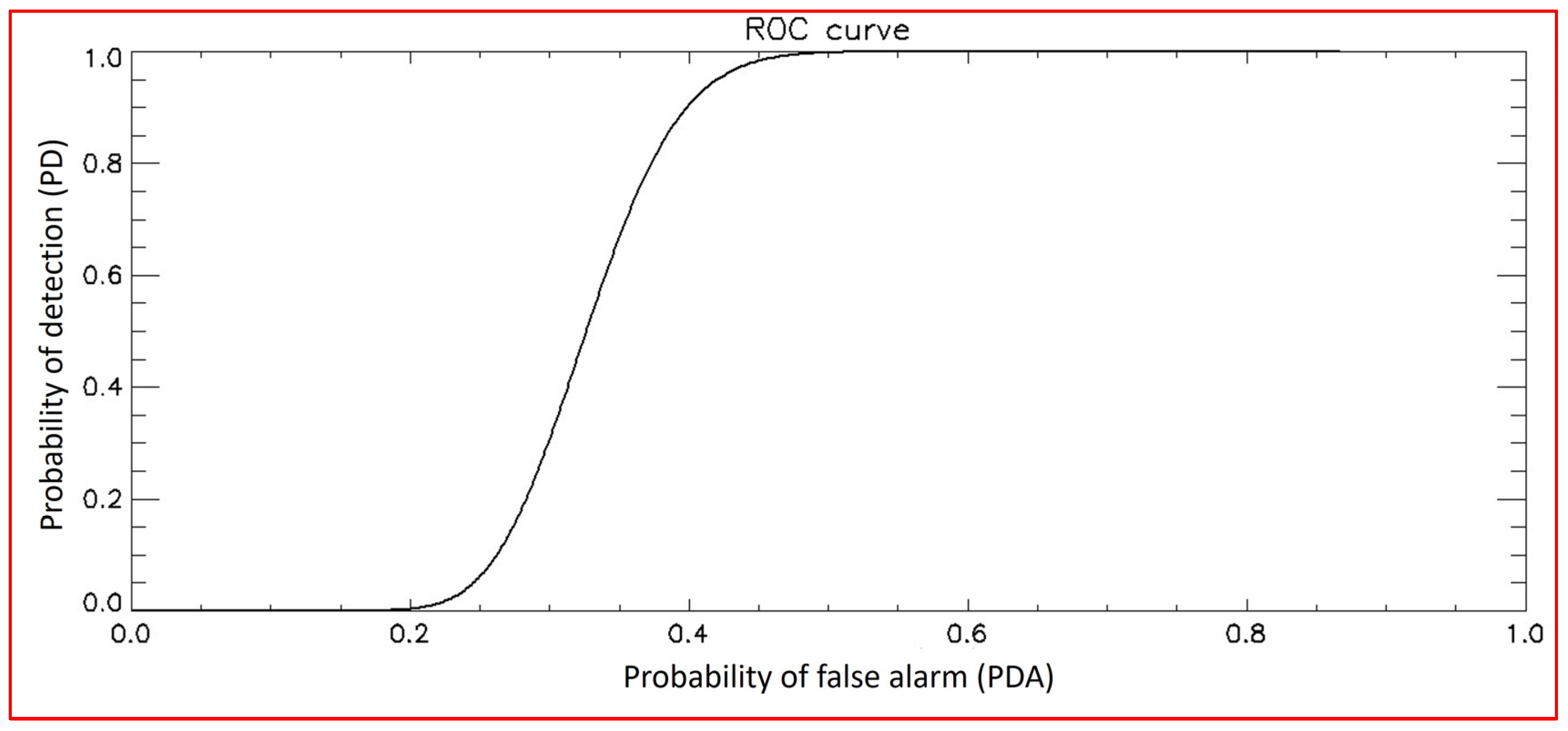
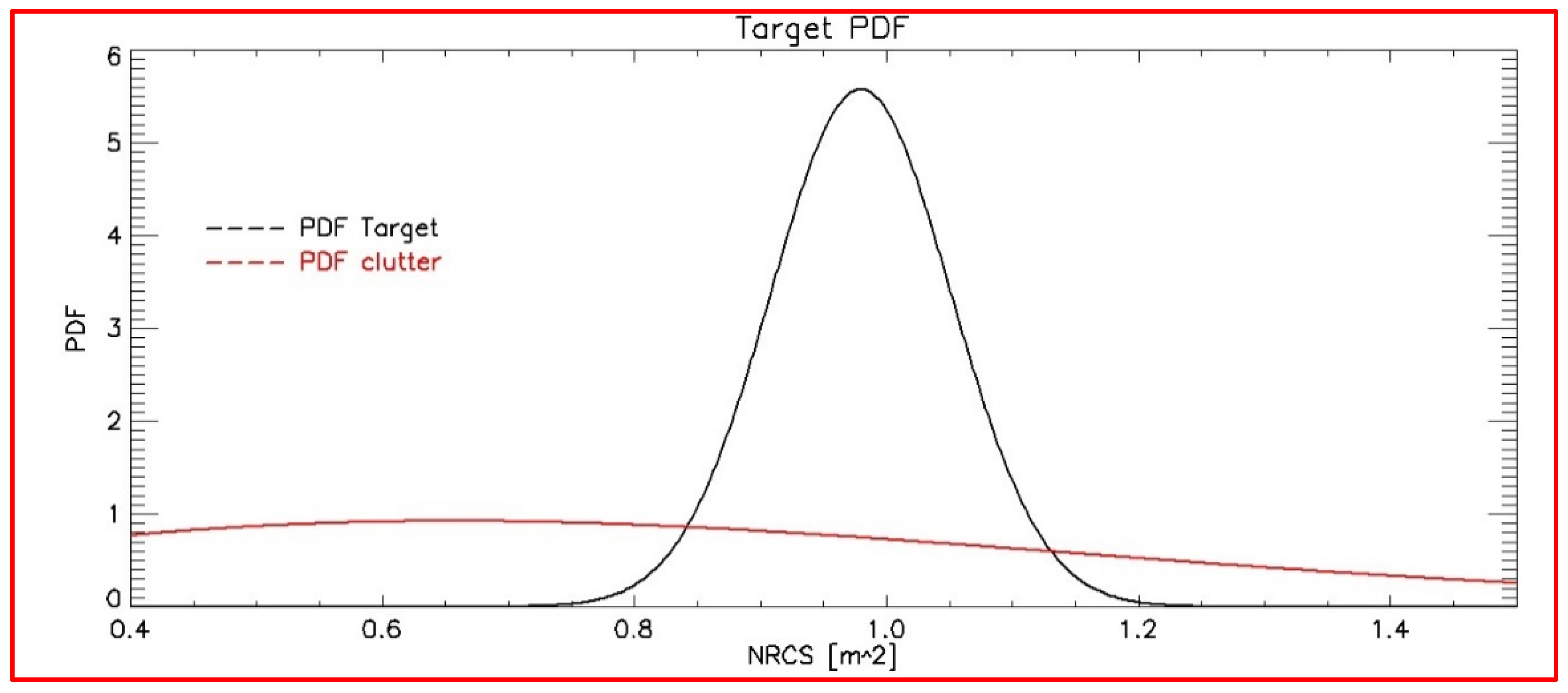
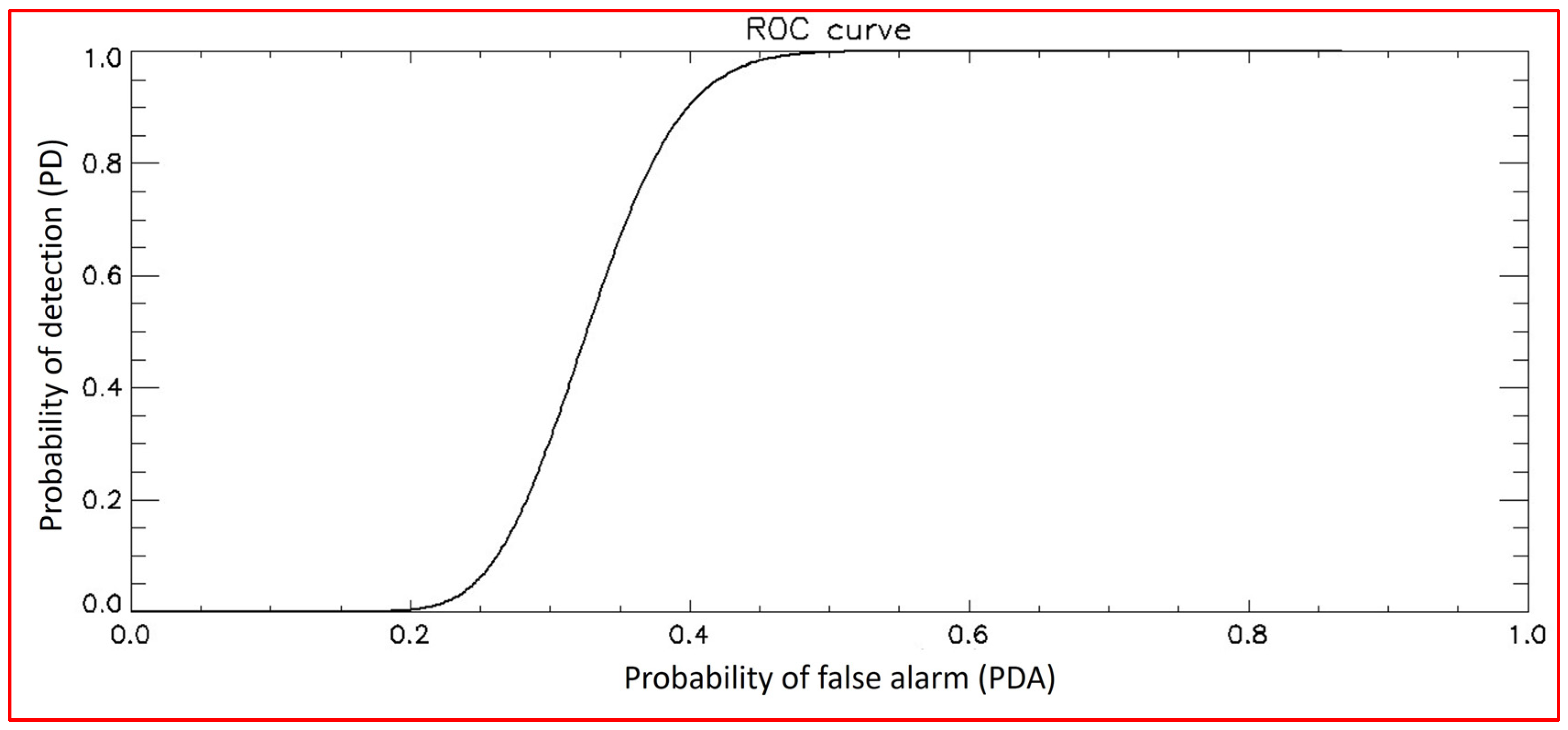
2.7. Probability of Detection of SGI in Rough Sea Conditions

In this section, we describe the detailed procedure aimed at calculating the probability of detection (PD) and the probability of false alarm (PFA) related to two SGI releases at two different ranges.

The aim is to estimate the PD and PFA for a single radar range cell based on the statistical properties of target signals and sea clutter.

Data preparation: Radar data for a specific range cell consist of signal amplitude readings, which include both SGI signals and sea clutter.

Step 1: PDF Estimation

Clutter PDF: Calculate the clutter PDF by first determining the standard deviation of the clutter data within the selected area. Assume a Rayleigh distribution (commonly used for sea clutter), and generate the PDF using these parameters.

Target PDF: Similarly, calculate the target PDF by analyzing the signal data from the cells where the target is present. Assume a Gaussian distribution for the target data and generate the PDF using the mean and standard deviation of these data.

Step 2: ROC Analysis for Threshold Determination

Implementing a Receiver Operating Characteristic (ROC) analysis to determine the optimal threshold that balances detection capabilities against false alarms: This involves plotting the PD against the PFA at various threshold levels and selecting the threshold that maximizes the detection rate while minimizing false alarms.

Step 3: PD and PFA Calculation

Integrating the target PDF from the optimal threshold to infinity to calculate the PD: This represents the probability that the target amplitude exceeds the threshold given the target is present.

PFA calculation: Similarly, integrate the clutter PDF from the optimal threshold to infinity to estimate the PFA. This represents the probability that the clutter amplitude exceeds the threshold when no target is present.

The results of this procedure are detailed in Section 3.

3. Results

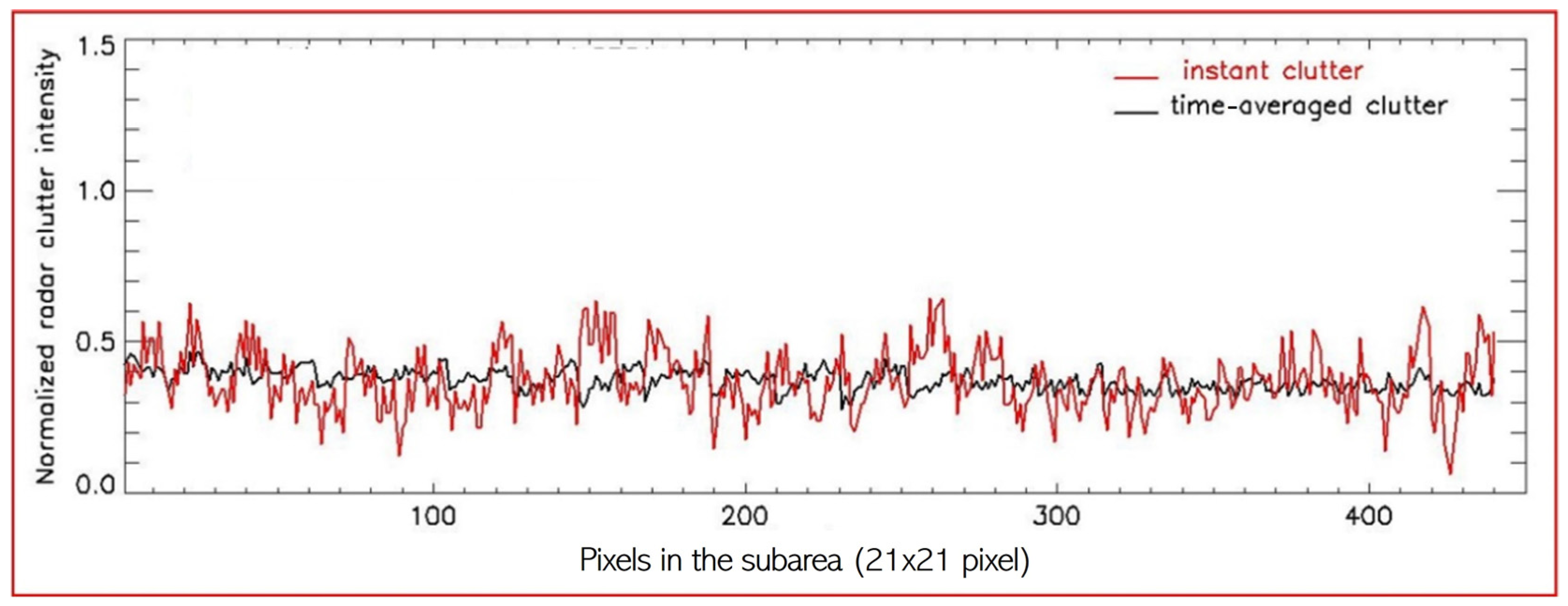
3.1. Radar Signal Intensity Analysis and Time-Based Data Processing

Figure 8 shows the radar intensities for targets T0, T1, T2 and T3 versus time, normalized with respect to the maximum radar intensity recorded during the first release (0.12 nautical miles) in the first measurement campaign.

The intensity spikes relating to targets T1 (red line), T2 (green line) and T3 (yellow line) correspond to the entry into the subarea of the inflatable dinghy from which the SGIs were released and are thus associated with the backscatter from the dinghy rather than from the targets. Given the craft’s high radar reflectivity, the radar recorded these events as a spike in the radar intensity of the area containing the targets until the craft exited the subarea.

As the second measurement campaign was carried out in the presence of rough seas and windy conditions, the mean clutter level was higher than in the calm sea conditions encountered in the first campaign, making it more difficult to distinguish between the target backscatter and the instantaneous clutter signal intensity.

As indicated above, this problem was overcome by the introduction of two innovations with respect to the procedure illustrated in [51]. The first consists of the introduction of a procedure for the dynamic extraction of the subareas containing the targets, aimed at automatically compensating for the targets’ drift. This procedure ensures that the subareas are always perfectly centered on the SGIs in order to maximize the signal backscattered by the targets. The dynamic extraction of the subarea is carried out by measuring the targets’ speed, which is calculated from the sequence of radar images and used to “follow” the targets over time. This procedure maximized the target time correlation. In Section 3.3, the speed of the targets will be compared with the speed of the surface current, highlighting that the SGIs have the same speed as the field of surface currents. The following steps describe the detailed procedure:

Step 1: The target is first observed in a certain period of time (20 consecutive images), and the displacement (Δs) covered in this period (Δt) is calculated.

Step 2: The movement speed is calculated using v = Δs/Δt.

Step 3: The determined speed is used to move the subarea containing the target so that it is always at the center of it.

The second innovation consists of the introduction of a decluttering procedure based on the temporal averaging of radar images, which exploits the targets’ time correlation and the lack of time correlation of the clutter. In this specific case, the time average was applied to n = 20 consecutive radar images. The results are illustrated in Figure 9, Figure 10, Figure 11, Figure 12 and Figure 13.

Figure 9 and Figure 10 depict two images acquired by the radar and represented in terms of the NRCS using the procedure outlined in Section 2.6. Figure 9 depicts the instantaneous radar image of the antenna coverage area on the left, while the right side of the figure shows zoomed views of the survey area, the area containing targets T0 and T1, and the individual targets T0 and T1. As can be seen from the instantaneous radar image, the clutter level makes it very difficult to distinguish the targets.

Figure 10 shows the same representation of the antenna coverage area and zoomed views after time averaging. In particular, the left image refers to the time average of 20 consecutive images. Thanks to the averaging procedure, the time-correlated targets are clearly visible and thus distinguishable from the time-uncorrelated clutter.

To make the target and clutter subareas comparable, the area including average clutter has been extracted at the same range as the subareas including the targets in order to account for the radiometric attenuation along the range (see the white boxes in Figure 9 and Figure 10).

In Figure 11, the red line represents the instantaneous NRCS clutter, while the black line represents the NRCS clutter after averaging. The X-axis shows the pixel index belonging to the subarea (21 × 21 pixels) selected for the clutter measurement. The figure also shows the means and standard deviations of the two curves.

For the completeness of exposition, the results presented in Figure 11 in terms of the NRCS have also been depicted in terms of the normalized radar signal intensity (see Figure 12), enabling a comparison with the radar signal intensities backscattered by targets during the first measurement campaign (see Figure 8). A comparison of the average clutter intensity with the backscatter intensity from targets T0 and T1 in Figure 8 shows that the system is able to detect the presence of the two targets whose intensity exceeds the time-averaged clutter level in the weather and sea conditions encountered in the second measurement campaign. It is also clear that if the methodology employed in the first campaign had been used in these weather and sea conditions, the system would not have been able to distinguish between the backscatter from the two targets and the higher-intensity instantaneous clutter.

Lastly, although the fact that the targets are time-correlated and the clutter is not time-correlated means that the mean time-averaged clutter NRCS is comparable to that of the mean instantaneous clutter NRCS (see Figure 11), the standard deviation of the time-averaged clutter NRCS (0.10) is significantly lower than that of instantaneous clutter (0.30).

Starting from these results, we can say that the time-averaging operation introduced here makes it possible to distinguish between the targets’ NRCSs and the time-averaged clutter NRCS under the weather conditions obtained in the second campaign. This is well illustrated in Figure 13, which compares the NRCSs of targets T0 and T1 with the time-averaged clutter NRCS and the instantaneous clutter NRCS.

3.2. The PD and PFA for the Two SGI Releases

Regarding the calculation of the PD (probability of detection) and PFA (probability of false alarm), the procedure outlined in Section 2.7 was applied to the cells containing the SGIs during the two releases, with respective ranges of 0.12 and 0.27 nautical miles. For the computation of the PDFs (Probability Density Functions) of the SGIs and clutter relative to the release at the shorter range (0.12 NM), the areas indicated in Figure 11 by “clutter”, “T0” and “T1” were selected. Figure 14 displays the plots of the two PDFs.

The following image (Figure 15) displays the ROC curve obtained by varying the threshold between 0 and 2.

From the ROC curve, the optimal threshold was extracted as a trade-off between the PD and PFA, resulting in a value of 1.33 m² (the value 1.33 was determined using step 2 of the procedure described in Section 2.7 for choosing the optimal threshold). Using this threshold, the optimal PD and PFA were calculated as follows: PD = 0.90 and PFA = 0.23, respectively (these values were obtained by integrating the PDF curves of the target and the clutter from the value of 1.33 up to infinity). The same procedure was subsequently applied to target T0 corresponding to the second release, which, at the time of measurement, was located at a range of 0.27 NM. The following image (Figure 16) displays the area containing targets T0 and T1 and the clutter area for PDF calculations.

Once again, the PDFs of the target and clutter were calculated in this case as well, and they are displayed in Figure 17.

From the PDFs, the ROC curve was calculated (see Figure 18), and the optimal threshold was estimated at 0.84 m².

Subsequently, PD = 0.97 and PFA = 0.44 were computed. As anticipated, with the increase in range, the probability of false alarm increases.

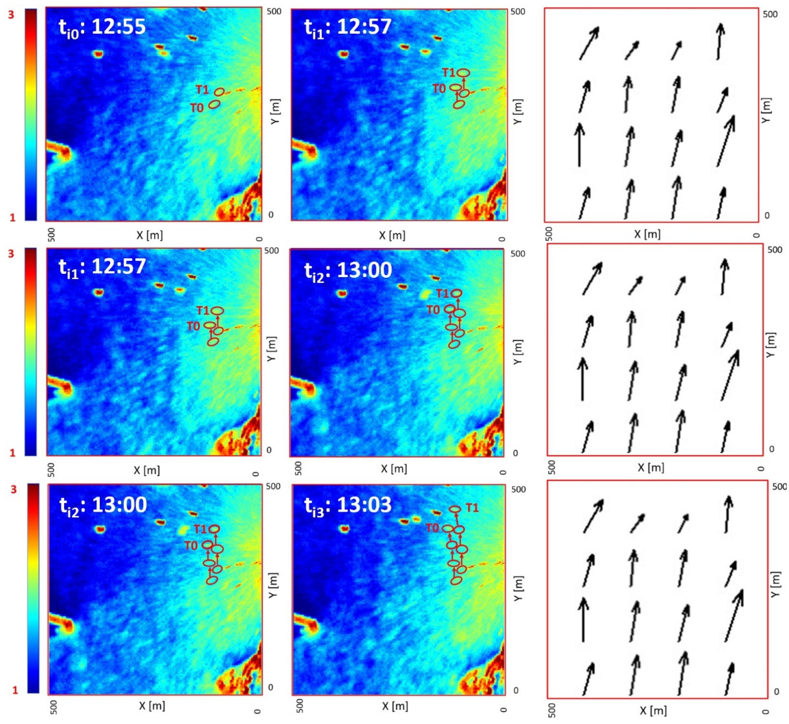
3.3. Target Movement Analysis

T0 and T1 target movements during the second measurement campaign were also analyzed. Similar to the first measurement campaign [51], the analysis of the target movement was also compared with the field of surface currents measured by the radar system (for the method used to estimate surface currents from X-band radar data, see [58]). The movements of targets T0 and T1 were measured from radar images for different instants of time. Figure 19 shows target movements between time instants ti₀–ti₁, ti₁–ti₂ and ti₂–ti₃ (the first two columns on the left). The red arrows in the figures indicate target movements from one instant to the next. The third column from the left shows the current field in the survey area provided by the wave radar system for the time interval in question (for the method used to estimate surface currents from X-band radar data, see [58]). This current measurement was generated by averaging the module of the current intensity in the survey area, eliminating the spikes above double the average and below half the average. The calculated average speed and direction of the current in the survey area were 0.17 m/s and 0.18°N, respectively. As can be inferred from the figure, target movements tend to follow those of the surface currents very closely in the rough sea conditions found in the second measurement campaign.

Table 2. The target speed and direction of movement during the first release (0.12 NM) of the second measurement campaign.

	Speed ti0–ti1 (m/s)	Direction ti0–ti1 (°N)	Speed ti1–ti2 (m/s)	Direction ti1–ti2 (°N)	Speed ti2–ti3 (m/s)	Direction ti2–ti3 (°N)
T0	0.16	7.6	0.18	−6,7	0.18	−6.7
T1	0.18	0°	0.2	−8.9	0.2	−8.9

shows target speeds and the associated directions of movement with respect to the north between the time instants ti₀–ti₁, ti₁–ti₂ and ti₂–ti₃, calculated from the observed target positions at each instant (the time between one time index and the next is known from the radar antenna rotation period).

Measurements between time instants were used to calculate the average speed and the average direction of the two targets T0 and T1, which were, respectively, ST0_Ave = 0.17 m/sec and DT0_Ave = −2° for target T0, and ST1_Ave = 0.19 m/sec DT0_Ave = −6° for target T1. The target speeds and directions of movement were compared with the speed and direction of the surface current in the survey area (see

Table 3. Comparison between average target speed and direction of movement and average current speed and direction of movement.

	T0	T1	Current
Speed	0.17	0.19	0.18
Direction	−2°N	−6°N	0.2°N

), confirming what can be seen graphically in Figure 19, i.e., that target movements follow the surface currents very closely.

4. Discussion

As regards X-band radar’s ability to identify and recognize SGI modules, this study found that with the calm seas and almost no wind in the first measurement campaign, targets T0, T1, T2 and T3 were all clearly visible from the radar data and were easily distinguished from average sea clutter (Figure 8).

In the second campaign, the time-based radar data analysis procedure illustrated in Section 3.1 made it possible to overcome the limits of the method proposed in [51] so that the targets could be correctly identified even with heavy seas and winds. As can be seen in Figure 10 and Figure 11, the NRCS of the targets averaged over time are greater than NRCS of the clutter averaged over time, thus making the targets detectable by the radar.

This is confirmed by Figure 9, where the clutter level in the instantaneous radar image obtained with the procedure used in the first campaign (and represented in this case in terms of the NRCS) is so high that it does not allow the targets to be distinguished (the instantaneous target NRCS falls within the range of variation of the instantaneous clutter NRCS). By contrast, the targets are clearly visible in Figure 10 for the first release (0.12 NM) and Figure 16 for the second release (0.27 NM), which depicts the time-averaged radar image, as their NRCSs are higher than the time-averaged NRCS clutter.

Accordingly, the conditions characterizing the second campaign can be regarded as a good approximation of the limit sea state threshold beyond which the target backscatter intensity is masked by the mean clutter, thus making it very difficult to use radar for monitoring SIGs. In addition, as the proposed method has been successfully tested for targets moving within a distance of 0.27 nautical miles from the antenna (beyond this limit, the method is ineffective, since the backscattered target signal decreases with the distance from the radar antenna until it is indistinguishable from the time-averaged clutter intensity), 0.27 nautical miles can be regarded as the limit distance threshold under which wave radar can effectively identify targets floating on the sea surface in the weather conditions of the second campaign.

The calculation of the probability of detection and probability of false alarm, as illustrated in Section 3.2, as we would logically expect, has highlighted that the PFA increases with the range.

Moving to an analysis of target movements in the second campaign, which, for the sake of clarity, has been limited to just the first release (0.12 NM), Figure 19 suggests that wave radar can effectively track targets even under the sea conditions encountered in this campaign. As the figure shows, targets T0 and T1 are clearly visible both in space and in time and move in the same direction as the current. This is confirmed analytically by the data reported in Table 2 and Table 3, which demonstrate that the targets move following the same direction as the surface current and assume speeds entirely similar to those recorded for the current during the campaign.

Conversely, it was not possible to determine whether the wind influences target movement, as the wind direction was roughly comparable to that of the surface current.

5. Conclusions

The study presented here was carried out to (1) assess the capability of an X-band radar system to detect and monitor small aggregations of litter consisting mostly or entirely of plastic floating in the sea; (2) determine X-band radar systems’ limits of use in terms of target distance from the antenna, especially as sea conditions worsen; and (3) identify the sea state limit threshold beyond which the target backscatter intensity is comparable to that of the average sea clutter and can thus be confused with it, making targets impossible to detect.

The analysis of the data acquired during the measurement campaign with calm seas and little or no wind showed that the characteristics of the target backscatter are distinct, and therefore discriminable, from backscatter from other sources. In these weather and sea conditions, empirical data demonstrated that X-band radar was capable of distinguishing the experimental SGIs within a maximum distance of 0.39 nautical miles from the receiving antenna. If the targets are beyond this distance, backscatter signal strength is attenuated to the point where it can no longer be distinguished from mean sea clutter.

With rough seas and wind, this study found that wave radar can distinguish the signal from the targets in the second measurement campaign within a maximum of 0.27 nautical miles (beyond this distance, the proposed method is ineffective for the specific targets used under these conditions, as the target backscatter intensity is too low to be distinguished from clutter intensity).

The sea and weather conditions encountered in the second campaign were found to be the threshold beyond which X-band radar is of little use for detecting and monitoring aggregations of floating litter.

This paper includes five innovations with respect to [51]. First, an automated target tracking procedure (for target drifting compensation), which ensures that the subarea is always centered on the SGIS, maximizes the target time correlation. Second, a data time-averaging step (decluttering) was introduced to better detect targets inside the clutter. Third, the results of the second measurement campaign have been represented in terms of the NRCS instead of the normalized radar signal intensity. Fourth, the PD and PFA were calculated as a function of range, demonstrating that the false alarm probability increases with increasing range. Fifth, the analysis of the target movements has been compared with the surface current field estimated by the X-band radar system.

The possibility of measuring the speed and direction of small islands of floating litter, even with rough seas and wind, can open up an interesting line of research for future activities.

References

1. Beaumont, N.J.; Aanesen, M.; Austen, M.C.; Börger, T.; Clark, J.R.; Cole, M.; Hooper, T.; Lindeque, P.K.; Pascoe, C.; Wyles, K.J. Global Ecological, Social and Economic Impacts of Marine Plastic. Mar. Pollut. Bull. 2019, 142, 189–195. [Google Scholar] [CrossRef] [PubMed]
2. Lebreton, L.; Slat, B.; Ferrari, F.; Sainte-Rose, B.; Aitken, J.; Marthouse, R.; Hajbane, S.; Cunsolo, S.; Schwarz, A.; Levivier, A.; et al. Evidence that the Great Pacific Garbage Patch is Rapidly Accumulating Plastic. Sci. Rep. 2018, 8, 4666. [Google Scholar] [CrossRef] [PubMed]
3. Derraik, J.G.B. The Pollution of the Marine Environment by Plastic Debris: A Review. Mar. Pollut. Bull. 2002, 44, 842–852. [Google Scholar] [CrossRef] [PubMed]
4. Sheavly, S.B.; Register, K.M. Marine Debris & Plastics: Environmental Concerns, Sources, Impacts and Solutions. J. Polym. Environ. 2007, 15, 301–305. [Google Scholar]
5. Barnes, D.K.A.; Galgani, F.; Thompson, R.C.; Barlaz, M. Accumulation and Fragmentation of Plastic Debris in Global Environments. Philos. Trans. R. Soc. Lond. B Biol. Sci. 2009, 364, 1985–1998. [Google Scholar] [CrossRef] [PubMed]
6. Andrady, A.L. Microplastics in the Marine Environment. Mar. Pollut. Bull. 2011, 62, 1596–1605. [Google Scholar] [CrossRef] [PubMed]
7. Obbard, R.W.; Sadri, S.; Wong, Y.Q.; Khitun, A.A.; Baker, I.; Thompson, R.C. Global Warming Releases Microplastic Legacy Frozen in Arctic Sea Ice. Earth’s Future 2014, 2, 315–320. [Google Scholar] [CrossRef]
8. Suaria, G.; Berta, M.; Griffa, A.; Molcard, A.; Özgökmen, T.M.; Zambianchi, E.; Aliani, S. Dynamics of Transport, Accumulation, and Export of Plastics at Oceanic Fronts. In Chemical Oceanography of Frontal Zones. The Handbook of Environmental Chemistry; Belkin, I.M., Ed.; Springer: Berlin/Heidelberg, Germany, 2021; Volume 116. [Google Scholar]
9. Villarrubia-Gómez, P.; Cornell, S.E.; Fabres, J. Marine Plastic Pollution as a Planetary Boundary Threat—The Drifting Piece in the Sustainability Puzzle. Mar. Pol. 2018, 96, 213–220. [Google Scholar] [CrossRef]
10. Thompson, R.C.; Moore, C.J.; vom Saal, F.S.; Swan, S.H. Plastics, the Environment and Human Health: Current Consensus and Future Trends. Phil. Trans. R. Soc. B 2009, 364, 2153–2166. [Google Scholar] [CrossRef]
11. Thevenon, F.; Carroll, C.; Sousa, J. (Eds.) Plastic Debris in the Ocean: The Characterization of Marine Plastics and Their Environmental Impacts, Situation Analysis Report; IUCN: Gland, Switzerland, 2014. [Google Scholar]
12. Boucher, J.; Friot, D. Primary Microplastics in the Oceans: A Global Evaluation of Sources; IUCN: Gland, Switzerland, 2017. [Google Scholar]
13. Bertrand, J.; Souplet, A.; Gil De Sola, L.; Relini, G.; Politou, C.Y. International Bottom Trawl Survey in the Mediterranean (Medits). Instruction Manual, Version 5. 2007. Available online: https://www.sibm.it/SITO%20MEDITS/file.doc/Medits-Handbook_V5-2007.pdf (accessed on 14 January 2024).
14. Cheshire, A.C.; Adler, E. UNEP/IOC Guidelines on Survey and Monitoring of Marine Litter; United Nations Environment Programme: Nairobi, Kenya, 2009; Available online: https://www.researchgate.net/publication/256186638_UNEPIOC_Guidelines_on_Survey_and_Monitoring_of_Marine_Litter (accessed on 14 January 2024).
15. Van Franeker, J.A.; Blaize, C.; Danielsen, J.; Fairclough, K.; Gollan, J.; Guse, N.; Hansen, P.L.; Heubeck, M.; Jensen, J.K.; Le Guillou, G.; et al. Monitoring Plastic Ingestion by the Northern Fulmar Fulmarus glacialis in the North Sea. Environ. Poll. 2011, 159, 2609–2615. [Google Scholar] [CrossRef]
16. Hidalgo-Ruz, V.; Gutow, L.; Thompson, R.C.; Thiel, M. Microplastics in the Marine Environment: A Review of the Methods used for Identification and Quantification. Environ. Sci. Technol. 2012, 46, 3060–3075. [Google Scholar] [CrossRef] [PubMed]
17. Claessens, M.; Van Cauwenberghe, L.; Vandegehuchte, M.B.; Janssen, C.R. New Techniques for the Detection of Microplastics in Sediments and Field Collected Organisms. Mar. Pollut. Bull. 2013, 70, 227–233. [Google Scholar] [CrossRef] [PubMed]
18. Hanke, G.; Galgani, F.; Werner, S.; Oosterbaan, L.; Nilsson, P.; Fleet, D.; Kinsey, S.; Thompson, R.; Van Franeker, J.A.; Vlachogianni, T.; et al. Guidance on Monitoring of Marine Litter in European Seas; EUR–Scientific and Technical Research Series; Publications Office of the European Union: Luxembourg, 2013. [Google Scholar]
19. Galgani, F.; Hanke, G.; Werner, S.; De Vrees, L. Marine Litter within the European Marine Strategy Framework Directive. ICES J. Mar. Sci. 2013, 70, 1055–1064. [Google Scholar] [CrossRef]
20. Hoornweg, D.; Bhada-Tata, P. What a Waste: A Global Review of Solid Waste Management; Urban Development Series; Knowledge Papers No. 15; World Bank: Washington, DC, USA, 2012. [Google Scholar]
21. Kikaki, A.; Karantzalos, K.; Power, C.A.; Raitsos, D.E. Remotely Sensing the Source and Transport of Marine Plastic Debris in Bay Islands of Honduras (Caribbean Sea). Remote Sens. 2020, 12, 1727. [Google Scholar] [CrossRef]
22. Nihei, Y.; Yoshida, T.; Kataoka, T.; Ogata, R. High-Resolution Mapping of Japanese Microplastic and Macroplastic Emissions from the Land into the Sea. Water 2020, 12, 951. [Google Scholar] [CrossRef]
23. Martinez-Vicente, V.; Clark, J.; Corradi, P.; Aliani, S.; Arias, M.; Bochow, M.; Bonnery, G.; Cole, M.; Cozar, A.; Donnelly, R.; et al. Measuring Marine Plastic Debris from Space: Initial Assessment of Observation Requirements. Remote Sens. 2019, 11, 2443. [Google Scholar] [CrossRef]
24. Topouzelis, K.; Papageorgiou, D.; Karagaitanakis, A.; Papakonstantinou, A.; Ballesteros, M. Remote Sensing of Sea Surface Artificial Floating Plastic Targets with Sentinel-2 and Unmanned Aerial Systems (Plastic Litter Project 2019). Remote Sens. 2020, 12, 2013. [Google Scholar] [CrossRef]
25. Goddijn-Murphy, L.; Dufaur, J. Proof of Concept for a Model of Light Reflectance of Plastics Floating on Natural Waters. Mar. Pollut. Bull. 2018, 135, 1145–1157. [Google Scholar] [CrossRef] [PubMed]
26. Goddijn-Murphy, L.; Peters, S.; van Sebille, E.; James, N.A.; Gibb, S. Concept for a Hyperspectral Remote Sensing Algorithm for Floating Marine Macro Plastics. Mar. Pollut. Bull. 2018, 126, 255–262. [Google Scholar] [CrossRef]
27. Goddijn-Murphy, L.; Williamson, B. On Thermal Infrared Remote Sensing of Plastic Pollution in Natural Waters. Remote Sens. 2019, 11, 2159. [Google Scholar] [CrossRef]
28. Maximenko, N.; Corradi, P.; Law, K.L.; van Sebille, E.; Garaba, S.P.; Lampitt, R.S.; Galgani, F.; Martinez-Vicente, V.; Goddijn-Murphy, L.; Veiga, J.M.; et al. Toward the Integrated Marine Debris Observing System. Front. Mar. Sci. 2019, 6, 447. [Google Scholar] [CrossRef]
29. Garcia-Garin, O.; Aguilar, A.; Borrell, A.; Gozalbes, P.; Lobo, A.; Penadés-Suay, J.; Raga, J.A.; Revuelta, O.; Serrano, M.; Vighi, M. Who’s better at spotting? A Comparison Between Aerial Photography and Observer-Based Methods to Monitor Floating Marine Litter and Marine Mega-Fauna. Environ. Pollut. 2020, 258, 1136. [Google Scholar] [CrossRef] [PubMed]
30. Garcia-Garin, O.; Getino, T.M.; Brosa, P.L.; Borrel, A.; Aguilar, A.; Robalino, R.B.; Cardona, L.; Vighi, M. Automatic Detection and Quantification of Floating Marine Macro-Litter in Aerial Images: Introducing a Novel Deep Learning Approach Connected to a Web Application. R. Environ. Pollut. 2021, 273, 116490. [Google Scholar] [CrossRef] [PubMed]
31. Felício, J.M.; Costa, T.S.; Vala, M.; Leonor, N.; Costa, J.R.; Marques, P.; Moreira, A.A.; Caldeirinha, R.F.S.; Matos, S.A.; Fernandes, C.A.; et al. Feasibility of Radar-based Detection of Floating Macroplastics at Microwave Frequencies. IEEE Trans. Ant. Prop. 2024, 1, 99. [Google Scholar] [CrossRef]
32. Veettil, B.K.; Quan, N.H.; Hauser, L.T.; Van, D.D.; Quang, N.X. Coastal and Marine Plastic Litter Monitoring Using Remote Sensing: A Review. Estuar. Coast. Shelf Sci. 2022, 279, 108160. [Google Scholar] [CrossRef]
33. Kako, S.; Morita, S.; Taneda, T. Estimation of Plastic Marine Debris Volumes on Beaches Using Unmanned Aerial Vehicles and Image Processing Based on Deep Learning. Mar. Pollut. Bull. 2020, 155, 111127. [Google Scholar] [CrossRef] [PubMed]
34. Garaba, S.P.; Dierssen, H.M. An Airborne Remote Sensing Case Study of Synthetic Hydrocarbon Detection Using Short Wave infrared Absorption Features Identified From Marine-Harvested Macro-and Microplastics. Remote Sens. Environ. 2018, 205, 224–235. [Google Scholar] [CrossRef]
35. Martin, C.; Parkes, S.; Zhang, Q.; Zhang, X.; McCabe, M.F.; Duarte, C.M. Use of Unmanned Aerial Vehicles for Efficient Beach Litter Monitoring. Mar. Pollut. Bull. 2018, 131, 662–673. [Google Scholar] [CrossRef]
36. Moy, K.; Neilson, B.; Chung, A.; Meadows, A.; Castrence, M.; Ambagis, S.; Davidson, K. Mapping Coastal Marine Debris Using Aerial Imagery and Spatial Analysis. Mar. Pollut. Bull. 2018, 132, 52–59. [Google Scholar] [CrossRef]
37. Fallati, L.; Polidori, A.; Salvatore, C.; Saponari, L.; Savini, A.; Galli, P. Anthropogenic Marine Debris Assessment with Unmanned Aerial Vehicle Imagery and Deep Learning: A Case Study Along the Beaches of the Republic of Maldives. Sci. Total Environ. 2019, 693, 133581. [Google Scholar] [CrossRef]
38. Evans, M.C.; Ruf, C.S. Toward the Detection and Imaging of Ocean Microplastics With a Spaceborne Radar. IEEE Trans. Geosci. Remote Sens. 2022, 60, 4202709. [Google Scholar] [CrossRef]
39. Themistocleous, K.; Papousta, C.; Michaelides, S.; Hadjimitsis, D. Investigating Detection of Floating Plastic Litter from Space Using Sentinel-2 Imagery. Remote Sens. 2020, 12, 2648. [Google Scholar] [CrossRef]
40. Basu, B.; Sannigrahi, S.; Basu, A.S.; Pilla, F. Development of Novel Classification Algorithms for Detection of Floating Plastic Debris in Coastal Waterbodies Using Multispectral Sentinel-2 Remote Sensing Imagery. Remote Sens. 2021, 13, 1598. [Google Scholar] [CrossRef]
41. Biermann, L.; Clewley, D.; Martinez-Vicente, V.; Topouzelis, K. Finding Plastic Patches in Coastal Waters Using Optical Satellite Data. Sci. Rep. 2020, 10, 5364. [Google Scholar] [CrossRef] [PubMed]
42. Kremezi, M.; Kristollari, V.; Karathanassi, V.; Topouzelis, K.; Kolokoussis, P.; Taggio, N.; Aiello, A.; Ceriola, G.; Barbone, E.; Corradi, P. Increasing the Sentinel-2 Potential for Marine Plastic Litter Monitoring Through Image Fusion Techniques. Mar. Pollut. Bull. 2022, 182, 113974. [Google Scholar] [CrossRef] [PubMed]
43. Guffogg, J.A.; Blades, S.M.; Soto-Berelov, M.; Bellman, C.J.; Skidmore, A.K.; Jones, S.D. Quantifying Marine Plastic Debris in a Beach Environment Using Spectral Analysis. Remote Sens. 2021, 13, 4548. [Google Scholar] [CrossRef]
44. Valdenegro-Toro, M. Submerged Marine Debris Detection with Autonomous Underwater Vehicles. In Proceedings of the International Conference on Robotics and Automation for Humanitarian Applications (RAHA 2016), Amritapuri, India, 18–20 December 2016; pp. 1–7. [Google Scholar]
45. Fulton, M.; Hong, J.; Islam, M.J.; Sattar, J. Robotic Detection of Marine Litter Using Deep Visual Detection Models. In Proceedings of the International Conference on Robotics and Automation (ICRA 2019), Montreal, QC, Canada, 20–24 May 2019; pp. 5752–5758. [Google Scholar]
46. Watanabe, J.; Shao, Y.; Miura, N. Underwater and Airborne Monitoring of Marine Ecosystems and Debris. J. Appl. Remote Sens. 2019, 13, 044509. [Google Scholar] [CrossRef]
47. Hurtos, N.; Palomeras, N.; Nagappa, S.; Salvi, J. Automatic Detection of Underwater Chain Links Using a Forward-Looking Sonar. In Proceedings of the 2013 MTS/IEEE OCEANS—BERGEN, Bergen, Norway, 14–19 June 2013; pp. 1–7. [Google Scholar]
48. Ge, Z.; Shi, H.; Mei, X.; Dai, Z.; Li, D. Semi-Automatic Recognition of Marine Debris on Beaches. Sci. Rep. 2016, 6, 25759. [Google Scholar] [CrossRef] [PubMed]
49. 49 Yuying, H.; Zhenpeng, G.; Daoji, L. LiDAR-based Quickly Recognition of Beach Debris. Haiyang Xuebao 2019, 41, 156–162. [Google Scholar]
50. Kataoka, T.; Murray, C.C.; Isobe, A. Quantification of Marine Macro-Debris Abundance Around Vancouver Island, Canada, Based on Archived Aerial Photographs Processed by Projective Transformation. Mar. Pollut. Bull. 2018, 132, 44–51. [Google Scholar] [CrossRef]
51. Serafino, F.; Bianco, A. Use of X-Band Radars to Monitor Small Garbage Islands. Remote Sens. 2021, 13, 3558. [Google Scholar] [CrossRef]
52. Savastano, S.; Cester, I.; Perpinya, M.; Romero, L. A First Approach to the Automatic Detection of Marine Litter in SAR Images Using Artificial Intelligence. In Proceedings of the IEEE International Geoscience and Remote Sensing Symposium (IGARSS 2022), Brussels, Belgium, 11–16 July 2022; pp. 8704–8707. [Google Scholar]
53. Broere, S.; van Emmerik, T.V.; González-Fernández, D.; Luxemburg, W.; Schipper, M.; Cozar, A.; Giesen, N. Towards Underwater Macroplastic Monitoring Using Echo Sounding. Front. Earth Sci. 2021, 9, 628704. [Google Scholar] [CrossRef]
54. Madricardo, F.; Ghezzo, M.; Nesto, N.; Kiver, W.J.M.; Faussone, G.C.; Fiorin, R.; Riccato, F.; Mackelworth, P.C.; Basta, J.; Pascalis, F.D.; et al. How to Deal with Seafloor Marine Litter: An Overview of the State-of-the-Art and Future Perspectives. Front. Mar. Sci. 2020, 9, 505134. [Google Scholar] [CrossRef]
55. Simpson, M.D.; Marino, A.; de Maagt, P.; Gandini, E.; de Fockert, A.; Hunter, P.; Spyrakos, E.; Telfer, T.; Tyler, A. Investigating the Backscatter of Marine Plastic Litter Using a Cand X-Band Ground Radar, during a Measurement Campaign in Deltares. Remote Sens. 2023, 15, 1654. [Google Scholar] [CrossRef]
56. Nieto Borge, J.C.; Guedes Soares, C. Analysis of Directional Wave Fields Using X-band Navigation Radar. Coast. Eng. 2000, 40, 375–391. [Google Scholar] [CrossRef]
57. Serafino, F.; Lugni, C.; Soldovieri, F. A Novel Strategy for the Surface Current Determination From Marine X-band Radar Data. IEEE Geosci. Remote Sens. Lett. 2010, 7, 231–235. [Google Scholar] [CrossRef]
58. Serafino, F.; Lugni, C.; Borge, J.C.N.; Zamparelli, V.; Soldovieri, F. Bathymetry Determination via X-Band Radar Data: A New Strategy and Numerical Results. Sensors 2010, 10, 6522–6534. [Google Scholar] [CrossRef] [PubMed]
59. Serafino, F.; Lugni, C.; Ludeno, G.; Arturi, D.; Uttieri, M.; Buonocore, B.; Zambianchi, E.; Budillon, G.; Soldovieri, F. REMOCEAN: A Flexible X-Band Radar System for Sea-State Monitoring and Surface Current Estimation. IEEE Geosci. Remote Sens. Lett. 2012, 9, 822–826. [Google Scholar] [CrossRef]
60. Yang, X.; Zhiyong, S.; Zaiqi, L.; Hao, W.; Qiang, F. Target Detection in Low Grazing Angle with Adaptive OFDM Radar. Intern. J. Antennas Propag. 2015, 2015, 147368. [Google Scholar]
61. Herselman, P.L.; Baker, C.J.; de Wind, H.J. An Analysis of X-Band Calibrated Sea Clutter and Small Boat Reflectivity at Medium-to-Low Grazing Angles. Modell. Proc. Radar Sign. Earth Obser. Spec. Issue 2008, 2008, 463741. [Google Scholar] [CrossRef]
Figure 1. X-band radar used for the measurement campaign (Google, Images ©2019 CNES).
Remotesensing 16 02101 g001
Figure 2. An aerial view of the survey area with the corresponding radar image overlaid (Google, Images ©2019 CNES).
Remotesensing 16 02101 g002
Figure 3. Details of the T0 and T1 targets used during the two measurement campaigns.
Remotesensing 16 02101 g003
Figure 4. The wave parameters and directional spectrum recorded by wave radar during the second measurement campaign.
Remotesensing 16 02101 g004
Figure 5. The wave height and direction recorded by the Gorgona wave buoy during the second measurement campaign.
Remotesensing 16 02101 g005
Figure 6. The wind direction and speed measured at the ISPRA tidal weather station in the port of Livorno.
Remotesensing 16 02101 g006
Figure 7. Details of the radar image that includes the presence of the vessel with a known RCS (Tc).
Remotesensing 16 02101 g007
Figure 8. Radar intensities of the targets during the first measurement campaign.
Remotesensing 16 02101 g008
Figure 9. An instantaneous radar image of the antenna coverage area, presented in terms of the NRCS.
Remotesensing 16 02101 g009
Figure 10. The time-averaged radar image of the coverage area, expressed in terms of the NRCS, calculated as the average of 20 consecutive images.
Remotesensing 16 02101 g010
Figure 11. A plot (red line) of the NRCS for the “Clutter” box in Figure 10 and a plot (black line) of the clutter intensity for the “Clutter” box in Figure 11.
Remotesensing 16 02101 g011
Figure 12. A plot (red line) of the (normalized) clutter intensity for the “Clutter” and a plot (black line) of the clutter intensity for the “Clutter”.
Remotesensing 16 02101 g012
Figure 13. A comparison between the NRCSs of targets T0 and T1, NRCS time-averaged clutter (black line) and NRCS instantaneous clutter (green line).
Remotesensing 16 02101 g013
Figure 14. The figure illustrates the Probability Density Functions (PDFs) of the target and clutter for the first release (0.12 NM).
Remotesensing 16 02101 g014
Figure 15. The figure depicts the ROC curve corresponding to the PDFs from Figure 15.
Remotesensing 16 02101 g015
Figure 16. The time-averaged radar image of the coverage area during the second release, expressed in terms of the NRCS.
Remotesensing 16 02101 g016
Figure 17. The image displays the PDFs of the target and clutter, respectively, pertaining to the second release (0.27 NM).
Remotesensing 16 02101 g017
Figure 18. The figure depicts the ROC curve corresponding to the PDFs from Figure 18.
Remotesensing 16 02101 g018
Figure 19. Movements of targets T0 and T1 close to the radar and their comparison with the surface current field.
Remotesensing 16 02101 g019