Semi-Tightly Coupled Robust Model for GNSS/UWB/INS Integrated Positioning in Challenging Environments

Abstract

Currently, the integration of the Global Navigation Satellite System (GNSS), Ultra-Wideband (UWB), and Inertial Navigation System (INS) has become a reliable positioning method for outdoor dynamic vehicular and airborne applications, enabling high-precision and continuous positioning in complex environments. However, environmental interference and limitations of single positioning sources pose challenges. Especially in areas with limited access to satellites and UWB base stations, loosely coupled frameworks for GNSS/INS and UWB/INS are insufficient to support robust estimation. Furthermore, within a tightly coupled framework, parameter estimations from different sources can interfere with each other, and errors in computation can easily contaminate the entire positioning estimator. To balance robustness and stability in integrated positioning, this paper proposes a comprehensive quality control method. This method is based on the semi-tightly coupled concept, utilizing the INS position information and considering the dilution of precision (DOP) skillfully to achieve complementary advantages in GNSS/UWB/INS integrated positioning. In this research, reliable position and variance information obtained by INS are utilized to provide a priori references for a robust estimation of the original data from GNSS and UWB, achieving finer robustness without increasing system coupling, which fully demonstrates the advantages of semi-tight integration. Based on self-collected data, the effectiveness and superiority of the proposed quality control strategy are validated under severely occluded environments. The experimental results demonstrate that the semi-tightly coupled robust estimation method proposed in this paper is capable of accurately identifying gross errors in GNSS and UWB observation data, and it has a significant effect on improving positioning accuracy and smoothing trajectories. Additionally, based on the judgment of the DOP, this method can ensure the output of continuous and reliable positioning results in complex and variable environments. Verified by actual data, under the conditions of severe sky occlusion and NLOS (Non-Line-of-Sight), compared with the loosely coupled GNSS/INS, the positioning accuracy in the E, N, U directions of the semi-tight coupled GNSS/INS proposed in this paper has improved by 37%, 46%, and 28%. Compared with the loosely coupled UWB/INS, the accuracy in the E and N directions of the semi-tight coupled UWB/INS has improved by 60% and 34%. In such environments, GNSS employs the RTD (Real-Time Differential) algorithm, UWB utilizes the two-dimensional plane-positioning algorithm, and the positioning accuracy of the semi-tight coupled robust model of GNSS/UWB/INS in the E, N, U directions is 0.42 m, 0.55 m, and 3.20 m respectively.

1. Introduction

As the field of unmanned systems expands its demand for environmental perception, target tracking, and cluster coordination, the provision of location services has rapidly shifted from relying on a single method to a multi-source fusion approach for positioning, navigation, and timing (PNT) [1,2]. This transition has given rise to a greater need for reliability, continuity, and availability in multi-source fusion navigation and positioning. Researching efficient robust estimation models is the key to achieving these requirements.

Currently, GNSS positioning technology is the primary means of outdoor high-precision positioning [3], boasting advantages such as ease of operation, all-weather capability, and continuous real-time monitoring [4]. However, in challenging environments such as urban canyons and dense forests, satellite signal propagation is prone to obstruction and multipath errors [5]. Particularly when the number of available satellites is limited, these conditions can lead to the formation of pseudorange gross errors, which are difficult to identify and robustly estimate within the GNSS single positioning source through statistical consistency principles.

To address the aforementioned issues, a classic solution is to integrate the GNSS with an INS to form a combined navigation system known as GNSS/INS. Under the effective constraints of the INS, more reliable gross error detection can be achieved, exhibiting a good complementarity between the two systems. Among the combinations of the two, there are common configurations such as loosely coupled (LC), tightly coupled (TC), deeply coupled (DC) [6], and the recently proposed semi-tightly coupled (STC) [7]. In all these configurations, the INS serves to constrain the positioning results of the GNSS. However, the utilization of measurement data differs in different combination methods, leading to varying impacts on the performance of the combined navigation system.

However, in denied environments where long stretches of road are obstructed by trees or buildings, the GNSS positioning system is unable to perform measurement updates due to obstruction, while the INS accumulates errors without assistance from other positioning technologies for correction [8]. Consequently, in such scenarios, the GNSS/INS system fails to achieve stable and reliable positioning for long durations.

Addressing the aforementioned issues, UWB positioning technology is considered as an effective complementary means in GNSS-denied environments, due to its ability to provide high-precision indoor/outdoor positioning, strong anti-interference, excellent penetration power, low power consumption, and insensitivity to obstruction by overhead obstacles [9,10]. The currently developed GNSS/UWB/INS integrated system has emerged as a reliable positioning solution for complex outdoor environments [11,12,13]. While research on quality control for this integrated system is relatively mature, there is still a lack of a simple and efficient unified robust estimation method, and the fusion model for this integrated navigation system remains to be further refined.

In summary, considering the diversity, complexity, and variability of navigation and positioning scenarios, as well as the limitations of single positioning sources, this paper is structured as follows: Section 2 provides an overview of existing GNSS/UWB/INS integrated positioning models and robust estimation theories. Section 3 explains in detail the semi-tightly coupled robust model proposed in this paper and derives corresponding formulas. Section 4 introduces the experimental methods and results of this paper to further validate the effectiveness of the proposed method. Section 5 summarizes the research of this paper and discusses future work in response to the limitations of this study.

2. Related Work

This section will review research progress in the field of GNSS/UWB/INS integrated navigation and introduce theories and methods that provide inspiration for the research in this paper.

To address the limitations of single positioning sources in complex environments, exploring the complementary characteristics of different sensors to enhance the robustness and continuity of positioning systems has increasingly become the focus of research in the field of navigation and positioning. Regarding the research on GNSS/UWB/INS integrated navigation, the challenges and existing solutions can be summarized in the following two points:

The first challenge is research on multi-sensor fusion frameworks. Depending on the measurement information used, multi-sensor navigation fusion methods can be summarized into loosely coupled and tightly coupled approaches [14]. (1) In the loosely coupled model, taking the GNSS/INS loosely coupled model as an example, the data processing flows of the GNSS and INS are independent, with the measurement vector being the difference in position or velocity between the GNSS and INS [15]. The structure is relatively simple. However, its premise is that all positioning sources must be able to provide positioning, making it vulnerable to failure when the number of available satellites is less than four [16]. Furthermore, the INS only corrects and constrains the GNSS positioning results in the result domain through variance, which relies on the confidence in the variance. However, in most cases, the variance of any positioning source cannot accurately reflect the actual error size [17], so even with rigorous robust methods, it cannot continuously output optimal results of integrated navigation. (2) In the tightly coupled model, the measurement vector includes the differences between the GNSS pseudorange, carrier phase, and Doppler data, and the corresponding INS calculations [18,19]. Compared to the loosely coupled approach, it has a higher information utilization rate and a correspondingly higher parameter estimation accuracy, and it can still complete integrated positioning with a smaller number of satellites [20]. However, due to the tight coupling between sources, any gross error from either side will affect the entire positioning estimator. Based on the above comparison, some scholars have proposed a semi-tightly coupled method that falls between loosely coupled and tightly coupled [21], where the INS provides positional prior information for assisted calculation. However, there is limited research on multi-source fusion systems with more than three sources, such as GNSS/UWB/INS, based on this semi-tightly coupled structure, and there is no comprehensive robust solution based on this structure. In addition, this paper examines how to utilize the precision factors of satellites and UWB base stations to achieve multi-source fusion quality control in challenging environments, which remains to be further studied.

The second challenge lies in the research on robust algorithms for observational data in complex environments. For GNSS/INS and UWB/INS, Kalman filtering is the most widely used parameter estimation method in the data-processing process [22]. However, due to the impact of complex sky and ground environments, the pseudorange gross errors of GNSS and NLOS (Non-Line-of-Sight) errors of UWB often affect the model accuracy, leading to unidentifiable biases in the filtering process [23,24]. To improve the robustness of navigation systems in dynamic environments, many scholars have conducted research on robust estimation for the GNSS. Commonly used equivalent weight functions include the Hampel weight function [25], Tukey weight function [26], Huber weight function [27], and IGG III scheme [28]. However, there is limited research on the threshold selection and elastic robust methods for the aforementioned robust methods. Additionally, in scenarios with a small number of UWB base stations, it is difficult to utilize the aforementioned statistical robust principles, and other gross error detection methods still need to be considered. Also, in challenging environments, the configurations of GNSS satellites and UWB base stations will largely reflect the reliability of the positioning results. A multi-source fusion quality control method that considers DOP values remains to be further studied.

3. The Proposed Model and Robust Method

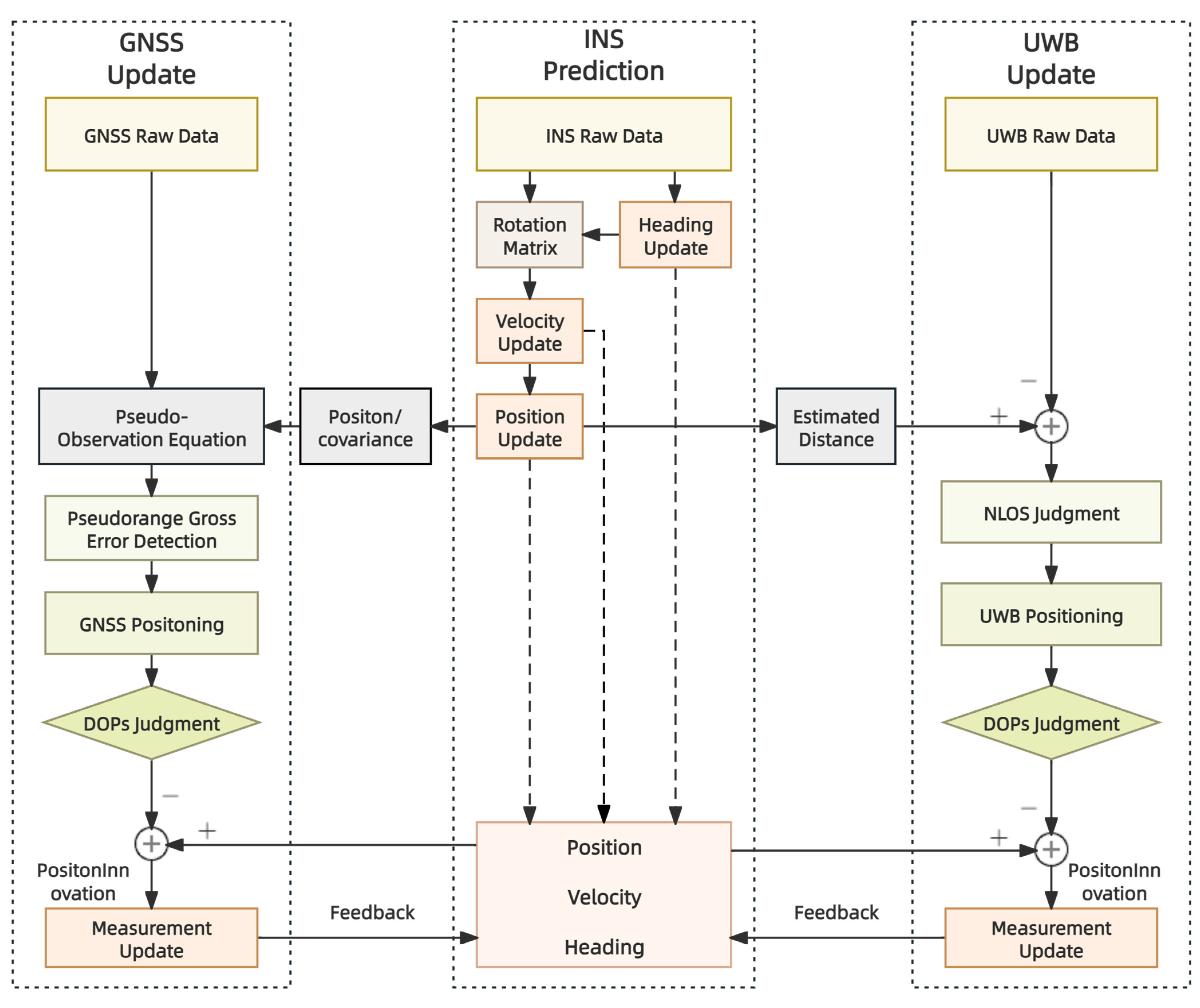
In this section, the proposed GNSS/UWB/INS semi-tightly coupled robust model will be explained. First, the system model of GNSS/UWB/INS integrated navigation will be introduced. Then, the robust methods for GNSS/INS and UWB/INS based on the semi-tightly coupled model will be discussed separately. The contribution of INS to robust estimation in the semi-tightly coupled model will be elaborated.

3.1. System Model

The semi-tightly coupled robust model proposed in this paper is illustrated in Figure 1. Based on the traditional loosely coupled framework, while borrowing the method of the close integration of information between different systems in tightly coupled configurations to enhance parameter estimation accuracy, the GNSS/UWB/INS semi-tightly coupled model introduces INS position information into the measurement update domains of both the GNSS and UWB, providing a priori references for gross error detection in the raw observation data of the GNSS and UWB. However, due to system differences, the robust methods for the GNSS and UWB, assisted by INS, are slightly different: (1) For the GNSS, the number of available satellites in each epoch is often more than 10; thus, the consistency principle and statistical testing methods between observations can be utilized for gross error identification. Here, the three-dimensional position and variance recursively obtained from the INS are introduced to construct pseudo-observation equations with other satellites, using standardized residuals as the basis for robustness. (2) For UWB, the number of base stations deployed on the test section is often less than 10. Furthermore, due to NLOS interference, there are fewer available observations in each epoch, rendering it unsuitable for statistical testing methods between data. In this case, the difference between the INS position and the distances calculated from each base station is compared with the original ranging values, using the absolute ranging difference as the basis for robustness.

Similar to the traditional centralized filtering model under the loosely coupled framework, in this GNSS/UWB/INS integrated navigation system, the dead reckoning of the INS serves as the main thread for state prediction, while the positioning results of the GNSS and UWB provide measurement updates. Both the GNSS and UWB perform error-based filtering with the INS in the positioning result domain. In this centralized filtering model, when either the GNSS or UWB measurement fails and leads to positioning interruption, the integrated navigation system can still rely on the other measurement system to achieve reliable positioning. The two systems complement each other, enabling the system to achieve complementary advantages in different testing environments.

In addition, the aforementioned model, in order to achieve reliable measurement updates in complex environments, takes into account the precision factor and determines whether the current DOP value meets the requirements before updating the GNSS and UWB measurements. This represents a more refined multi-source fusion quality control strategy.

3.2. State Prediction by INS

In the GNSS/UWB/INS integrated navigation system studied in this paper, considering the carrier’s motion state and the INS’s own drift, we select the three-dimensional position, velocity, attitude, gyroscope bias, accelerometer bias, gyroscope specific force, and accelerometer specific force as the state variables $\mathit{X}$ to be estimated, totaling 21 dimensional elements.

$$\mathit{X}={\left[\begin{array}{ccc}{\mathit{p}}_{3\times 1}& {\mathit{v}}_{3\times 1}& {\mathit{\psi }}_{3\times 1}\end{array}\begin{array}{ccc}\mathit{g}{\mathit{b}}_{3\times 1}& \mathit{a}{\mathit{b}}_{3\times 1}& \mathit{g}{\mathit{s}}_{3\times 1}\end{array}\mathit{a}{\mathit{s}}_{3\times 1}\right]}^T$$

(1)

In the Kalman filtering, the state and covariance prediction equations are:

$$\left\{\begin{array}{c}{\mathit{X}}_{k|k-1}={\Phi }_{k|k-1}·{\mathit{X}}_{k-1} \\ {\mathit{P}}_{k|k-1}={\Phi }_{k|k-1}·{\mathit{P}}_{k-1}·{\Phi }_{k|k-1}^T+{\mathit{Q}}_k \end{array}\right.$$

(2)

where ${\Phi }_{k|k-1}$ represents the state transition matrix from time $k-1$–to time $k$, and ${\mathit{X}}_{k-1}$ and ${\mathit{X}}_{k|k-1}$ represent the state estimate at time $k-1$ and the state prediction at time $k$, respectively. ${\mathit{P}}_{k-1}$ and ${\mathit{P}}_{k|k-1}$ represent the covariance estimate at time $k-1$ and the covariance prediction at time $k$, respectively. ${\mathit{Q}}_k$ represents theprocess noise at time $k$.

In this context, the partitioning of the state transition matrix $\Phi$ is as follows [29]:

$$\Phi =\left[\begin{array}{ccccccc}{\Phi }_{rr}& {\mathit{I}}_{3\times 3}& \mathbf{0}& \mathbf{0}& \mathbf{0}& \mathbf{0}& \mathbf{0}\\ {\Phi }_{vr}& {\Phi }_{vv}& \left[({\mathit{C}}_b^n{\mathit{f}}^b\right)\times ]& \mathbf{0}& {\mathit{C}}_b^n& \mathbf{0}& {\mathit{C}}_b^{n}diag\left({\mathit{f}}^b\right)\\ {\Phi }_{\varphi r}& {\Phi }_{\varphi v}& -\left({\mathit{\omega }}_{in}^n\right)& -{\mathit{C}}_b^n& \mathbf{0}& -{\mathit{C}}_b^n\left({\mathit{\omega }}_{ib}^n\right)& \mathbf{0}\\ \mathbf{0}& \mathbf{0}& \mathbf{0}& -\frac{1}{T_{gb}}{\mathit{I}}_{3\times 3}& \mathbf{0}& \mathbf{0}& \mathbf{0}\\ \mathbf{0}& \mathbf{0}& \mathbf{0}& \mathbf{0}& -\frac{1}{T_{ab}}{\mathit{I}}_{3\times 3}& \mathbf{0}& \mathbf{0}\\ \mathbf{0}& \mathbf{0}& \mathbf{0}& \mathbf{0}& \mathbf{0}& -\frac{1}{T_{gs}}{\mathit{I}}_{3\times 3}& \mathbf{0}\\ \mathbf{0}& \mathbf{0}& \mathbf{0}& \mathbf{0}& \mathbf{0}& \mathbf{0}& -\frac{1}{T_{as}}{\mathit{I}}_{3\times 3}\end{array}\right]$$

(3)

Among them, ${\mathit{C}}_b^n$ is the rotation matrix from the b-system to the n-system, ${\mathit{\omega }}_{ib}^n$ is the projection of the gyroscope’s original measurement vector in the n-system, ${\mathit{\omega }}_{in}^n$ represents the projection of the rotation angular velocity vector of the n-system relative to the i-system in the n-system, ${\mathit{f}}^b$ is the theoretical specific force perceived by the accelerometer in the b-system, $\left(·\right)\times$ represents the antisymmetric matrix of the corresponding vector, and $T_{gb}$, $T_{ab}$, $T_{gs}$, and $T_{as}$ are the relevant times of the first-order Gaussian Markov process.

Based on the mechanical arrangement principles of the INS, the predicted states such as position, velocity, and attitude for the current epoch can be obtained, serving as the benchmark for subsequent robust estimation and measurement updates. It should be noted that, due to the lever arm issue that may arise during the installation of testing equipment, the three-dimensional position of the INS should be converted to the antenna centers of the GNSS and UWB after the state prediction process to facilitate subsequent fusion.

3.3. STC Robust Method for GNSS/INS

In complex urban environments with limited satellite visibility due to obstructions from trees and buildings, the number of available GNSS satellites is often limited [30]. Although, in most cases, it can still meet the minimum requirement for the number of satellites required for pseudorange single-point positioning [31], relying solely on the statistical characteristics of observations from a single GNSS positioning source is prone to issues such as missing the detection of small gross errors and mistakenly rejecting normal observations. As a fully autonomous positioning source, the INS does not experience significant jumps or failures in a short period of time. It can utilize its relatively reliable position information to assist in improving the robustness of the GNSS positioning. This assisted robustness is mainly reflected in the construction of the GNSS observation equations. The following will explain this semi-tightly coupled robust method step by step.

3.3.1. GNSS Pseudorange Observation Equation

In the single-point positioning of the GNSS pseudorange, taking into account various error terms, the observation equation is:

$$P_r^s={\rho }_r^s+c·\left(\delta t_r-\delta t^s\right)+T_r^s+I_r^s+{\epsilon }_{P,r}^s$$

(4)

where $P_r^s$ represents the pseudorange observation value measured by receiver $r$ and satellite $s$, ${\rho }_r^s$ is the geometric distance between the receiver and the satellite, $c$ is the speed of light, $\delta t_r$ and $\delta t^s$ are the clock errors of the receiver and satellite, respectively, $T_r^s$ and $I_r^s$ are the tropospheric and ionospheric delay errors, and ${\epsilon }_{P,r}^s$ includes measurement noise and other errors. In Equation (4) above, the geometric distance ${\rho }_r^s$ can be expressed as:

$${\rho }_r^s=\sqrt{{\left(x^s-x_r\right)}^2+{\left(y^s-y_r\right)}^2+{\left(z^s-z_r\right)}^2}$$

(5)

In the equation, ${\mathit{X}}^s=\left[x^s,y^s,z^s\right]$ and ${\mathit{X}}_r=\left[x_r,y_r,z_r\right]$ represent the three-dimensional coordinates of the satellite and receiver, respectively. Generally, ${\mathit{X}}^s$ can be calculated by reading the ephemeris file, while ${\mathit{X}}_r$ represents the coordinates of the carrier to be estimated. According to the linearization principle of the Extended Kalman Filter (EKF), Equation (5) can be linearized. Typically, the approximate coordinates of the receiver are chosen as the expansion point, but in this case, the INS position at the same moment, after coordinate system conversion and lever arm compensation, ${\mathit{X}}_{ins}=\left[x_{ins},y_{ins},z_{ins}\right]$, can be used as the expansion point:

$${\rho }_r^s={\rho }_{r0}^s+l_r^s·\delta x_{ins}+m_r^s·\delta y_{ins}+n_r^s·\delta z_{ins}$$

(6)

$${\rho }_{r0}^s=\sqrt{{\left(x^s-x_{ins}\right)}^2+{\left(y^s-y_{ins}\right)}^2+{\left(z^s-z_{ins}\right)}^2}$$

(7)

The expansion coefficients are, respectively:

$$\left\{\begin{array}{c}{l}_r^s={\left.\frac{\partial {\rho }_r^s}{\partial x_{ins}}\right|}_{X_{ins}}=\frac{x_{ins}-x^s}{{\rho }_{r0}^s} \\ m_r^s={\left.\frac{\partial {\rho }_r^s}{\partial y_{ins}}\right|}_{X_{ins}}=\frac{y_{ins}-y^s}{{\rho }_{r0}^s}\\ n_r^s={\left.\frac{\partial {\rho }_r^s}{\partial z_{ins}}\right|}_{X_{ins}}=\frac{z_{ins}-z^s}{{\rho }_{r0}^s}\end{array}\right.$$

(8)

From this, we can derive that if there are N available satellites in the current epoch, the pseudorange observation equation in error form is given by Equation (9), which can be simplified as Equation (10):

$$\left[\begin{array}{c}{P}_r^1-{\rho }_{r0}^1+c·\delta t^1-T_r^1-I_r^1\\ P_r^2-{\rho }_{r0}^2+c·\delta t^2-T_r^2-I_r^2\\ ⋮\\ P_r^N-{\rho }_{r0}^N+c·\delta t^N-T_r^N-I_r^N\end{array}\right]=\left[\begin{array}{cccc}{l}_r^1& m_r^1& n_r^1& 1\\ l_r^2& m_r^2& n_r^2& 1\\ ⋮& ⋮& ⋮& ⋮\\ l_r^N& m_r^N& n_r^N& 1\end{array}\right]·\left[\begin{array}{c}\delta x_{ins}\\ \delta y_{ins}\\ \delta z_{ins}\\ c\delta t_r\end{array}\right]+{\mathit{\epsilon }}_{P,r}$$

(9)

$${\mathrm{L}}_{\mathrm{gnss}}={\mathrm{H}}_{\mathrm{gnss}}·\mathsf{\delta }\mathrm{X}$$

(10)

Using information such as the elevation angle-based weighting and signal-to-noise ratio, the observation noise matrix ${\mathit{R}}_{gnss}$ can be defined as:

$${\mathit{R}}_{gnss}={\left[\begin{array}{cccc}{\epsilon }_r^1& 0& 0& 0\\ 0& {\epsilon }_r^2& 0& 0\\ 0& 0& \ddots & 0\\ 0& 0& 0& {\epsilon }_r^n\end{array}\right]}_{N\times N}$$

(11)

3.3.2. INS Pseudo-Observation Equation

To incorporate the INS three-dimensional position coordinates into the aforementioned observation vector with a certain degree of confidence, while increasing the redundancy of the observation equation and preventing unidentifiable overall shifts in the observation system, thereby enhancing the accuracy of the subsequent robust estimation, a three-dimensional pseudo-observation equation is constructed, as shown in Equation (12). This pseudo-observation equation is then unified into the forms expressed in Equations (13) and (14):

$$\left\{\begin{array}{c}\delta x_{ins}=0\\ \delta y_{ins}=0\\ \delta z_{ins}=0\end{array}\right.$$

(12)

$$\left[\begin{array}{c}0\\ 0\\ 0\end{array}\right]=\left[\begin{array}{cccc}1& 0& 0& 0\\ 0& 1& 0& 0\\ 0& 0& 1& 0\end{array}\right]·\left[\begin{array}{c}\delta x_{ins}\\ \delta y_{ins}\\ \delta z_{ins}\\ c\delta t_r\end{array}\right]$$

(13)

$${\mathit{L}}_{ins}={\mathit{H}}_{ins}·\delta \mathit{X}$$

(14)

The noise ${\mathit{R}}_{ins}$ of this pseudo-observation equation corresponds precisely to the diagonal elements of the covariance matrix of the INS’s three-dimensional position after mechanical alignment, namely $co{v}_x$, $co{v}_y$, and $co{v}_z$:

$${\mathit{R}}_{ins}={\left[\begin{array}{ccc}co{v}_x& 0& 0\\ 0& co{v}_y& 0\\ 0& 0& co{v}_z\end{array}\right]}_{3\times 3}$$

(15)

3.3.3. (N + 3) Pseudo-Observation Equation

Furthermore, by combining the GNSS observation equation with the INS pseudo-observation equation, we obtain an (N + 3)-dimensional pseudo-observation equation incorporating INS position information, as shown in Equation (16), which is simplified and denoted as Equation (17):

$${\left[\begin{array}{c}{\mathit{L}}_{gnss}\\ {\mathit{L}}_{ins}\end{array}\right]}_{\left(N+3\right)\times 1}={\left[\begin{array}{c}{\mathit{H}}_{gnss}\\ {\mathit{H}}_{ins}\end{array}\right]}_{\left(N+3\right)\times 4}·\delta \mathit{X}$$

(16)

$$\mathit{L}=\mathit{H}·\mathit{\delta }\mathit{X}$$

(17)

The noise matrix $\mathit{R}$ of this (N + 3)-dimensional pseudo-observation equation can be expressed as:

$$\mathit{R}={\left[\begin{array}{cc}{\mathit{R}}_{gnss}& \\ & {\mathit{R}}_{ins}\end{array}\right]}_{\left(N+3\right)\times \left(N+3\right)}$$

(18)

3.3.4. Robust EKF with INS Constraints

Finally, when the number of available satellites satisfies $N>4$, the correction term $\delta \mathit{X}$ for the aforementioned state parameters can be solved. Influenced by the INS pseudo-observation equation and its weight, the $\delta \mathit{X}$ here will differ from that obtained solely from the N-dimensional observation equation of the GNSS. Instead, it will incorporate the correction term constrained by the INS, and the tightness of the constraint will be adjusted automatically based on the variance size: if the values in ${\mathit{R}}_{ins}$ are small, indicating a high confidence in the INS recursive position, then the INS coordinates will impose a tighter constraint on the correction term; conversely, if the values in ${\mathit{R}}_{ins}$ are large, the INS coordinates will impose a looser constraint on the correction term. Substituting $\delta \mathit{X}$ back into observation Equation (10) yields the N-dimensional posterior residual ${\mathit{V}}_{gnss}$:

$${\mathit{V}}_{gnss}={\mathit{L}}_{gnss}-{\mathit{H}}_{gnss}·\delta \mathit{X}$$

(19)

where the covariance ${\mathit{Q}}_{gnss}$ corresponding to the residual ${\mathit{V}}_{gnss}$ is:

$${\mathit{Q}}_{gnss}={\mathit{R}}_{gnss}+{\mathit{H}}_{gnss}·\mathit{P}·{\mathit{H}}_{gnss}^T$$

(20)

In the above equation, $\mathit{P}$ represents the covariance matrix of the state variables. Therefore, the normalized residual ${\check{\mathit{V}}}_{gnss}$ can be obtained as:

$${\check{\mathit{V}}}_{gnss}=\frac{{\mathit{V}}_{gnss}}{\sqrt{{\mathit{Q}}_{gnss}}}$$

(21)

To identify and adjust the weights of pseudorange outliers and their observation noises, according to the principle of equivalent weights, the noise matrix $\mathit{R}$ is replaced by the equivalent weight matrix $\overline{\mathit{R}}$, as shown in Equation (22):

$$\overline{\mathit{R}}=\left[\begin{array}{ccc}{\gamma }_{11}{R}_{11}& \dots & {\gamma }_{1N}{R}_{1N}\\ ⋮& \ddots & ⋮\\ {\gamma }_{N1}{R}_{N1}& \dots & {\gamma }_{NN}{R}_{NN}\end{array}\right]$$

(22)

where $R_{ij}$ represents the element in the i-th row and j-th column of the noise matrix $\mathit{R}$, and ${\gamma }_{ij}$ represents the robust factor for the element in the i-th row and j-th column. The robust factor is determined by the IGG III weight function [32,33], as shown in Equation (23):

$${\gamma }_{ii}=\left\{\begin{array}{c}1,\left|{\check{v}}_{gnss,i}\right|\le k_0\\ \frac{k_0}{\left|{\check{v}}_{gnss,i}\right|}{\left(\frac{k_1-\left|{\check{v}}_{gnss,i}\right|}{k_1-k_0}\right)}^2,\\ 0,\left|{\check{v}}_{gnss,i}\right|\ge k_1 \end{array}\right.k_0\le \left|{\check{v}}_{gnss,i}\right|\le k_1$$

(23)

where ${\check{v}}_{gnss,i} \left(i=1,2,\dots ,N\right)$ represents the i-th element in ${\check{\mathit{V}}}_{gnss}$, which corresponds to the normalized residual of the i-th satellite. $k_0$ and $k_1$ are the two key thresholds for the three-segment weight, and their selection should be based on the distribution of normalized residuals. In this paper, $k_0$ is chosen as 1.5 and $k_1$ as 5.0.

However, this robust method of adjusting observation weights based on posterior residuals poses a significant risk of misdetection, especially when the INS corresponding variance differs significantly from the actual error, leading to the possibility of normal measurements being erroneously assigned lower weights. Therefore, it is necessary to control the degree of robustness by introducing a robust elastic factor [33], which is primarily used to control the number of satellites rejected in this epoch. Specifically, as shown in Equation (24), two scaling factors $s_1$ and $s_2$ between 0 and 1 are introduced to control the maximum number of iterations $C_{max}$ for the IGG III robust loop [33], and the maximum number of satellites $N_{max}$ that can be classified into the IGG III rejection region.

$$\left\{\begin{array}{c}{C}_{max}=s_1·n_{obs} \\ N_{max}=s_2·n_{obs} \end{array}\right.$$

(24)

where $n_{obs}$ represents the number of satellites observed in that epoch, $s_1$ is typically set between 0.3 and 0.4, and $s_2$ is typically set between 0.1 and 0.2. By introducing the limits of $C_{max}$ and $N_{max}$, this can effectively prevent the IGG III from mistakenly excluding normal observations in the presence of some significant outliers, as shown in Figure 2. The upper part of the figure depicts the proportion of satellites in the three segments without the control of the elastic factor, showing that in some epochs, nearly half of the satellites are rejected. This is obviously due to the shift in the center of the residuals caused by a large number of small outliers. In such cases, it is difficult to distinguish between normal and faulty observations. Without control measures, it may lead to track drift or even positioning failure to converge. The lower part of the figure shows the proportion of satellites in the three segments after adding the control of the elastic factor. With the limits of $C_{max}$ and $N_{max}$, the proportion of satellites in the rejection domain of each epoch is below 15%, improving the robustness of the robustness estimation.

Under the control of the elastic factor, the equivalent weight matrix $\overline{\mathit{R}}$ obtained from Equation (22) is substituted for the noise matrix in the EKF to complete the measurement update of the GNSS. This realizes the detection of gross errors based on INS position domain information assistance. The subsequent experimental section will verify the effectiveness of this semi-tightly integrated robust method.

3.4. STC Robust Method for UWB/INS

In narrow road sections with dense human flow and piles of debris, the accuracy and stability of UWB positioning are significantly influenced by factors such as the configuration of base stations, NLOS errors, and the motion state of the carrier. It is difficult to overcome these obstacles with a single UWB positioning source, and therefore, the introduction of other continuous and reliable positioning methods is necessary. Similar to the principle of GNSS/INS integrated navigation, the INS can provide relatively reliable position constraints within a short period of time. However, unlike the GNSS, UWB has a smaller number of base stations, which is not suitable for statistical consistency checks between data. Therefore, its position information can be converted into distance information and compared with the original ranging measurements to achieve a more accurate NLOS error detection [34]. Below, we will sequentially introduce the semi-tightly integrated error identification process.

3.4.1. Two-Dimensional Distance Calculated by INS

Since the aforementioned UWB is only used for two-dimensional plane positioning, we only consider the two-dimensional plane coordinates obtained by the INS at time $k$, denoted as $x_{ins}\left(k\right)$ and $y_{ins}\left(k\right)$. It is worth noting that distances are calculated based on coordinate differences, so all position coordinates related to distance should be converted to the ECEF coordinate system. The geometric distances between the INS-estimated position and each UWB base station are calculated as follows:

$$d_i^{ins}\left(k\right)=\sqrt{{\left(x_{ins}\left(k\right)-x_{base}\left(i\right)\right)}^2+{\left(y_{ins}\left(k\right)-y_{base}\left(i\right)\right)}^2}$$

(25)

where $x_{base}\left(i\right)$ and $y_{base}\left(i\right)$ are the three-dimensional coordinates of the i-th base station, and $d_i^{ins}\left(k\right)$ represents the geometric distance between the INS-estimated position at time $k$ and the i-th base station.

3.4.2. Two-Dimensional Distance Measured by UWB

If there is a difference between the heights of the vehicle-mounted antenna and the base station antenna, the actual UWB ranging value should be corrected to obtain the ranging value $d_i^{uwb}\left(k\right)$ within the two-dimensional plane:

$$d_i^{uwb}\left(k\right)=\sqrt{d_i^2\left(k\right)-{\left(h_0-z_{base}\left(i\right)\right)}^2}$$

(26)

where $d_i\left(k\right)$ is the actual ranging value of the i-th base station, and $\left(h_0-z_{base}\left(i\right)\right)$ represents the difference in height between the vehicle-mounted antenna and the base station antenna.

3.4.3. NLOS Judgment Statistics

Based on this, an NLOS discrimination statistic is constructed, and a discrimination threshold is set:

$$\Delta d_i\left(k\right)=d_i^{ins}\left(k\right)-d_i^{uwb}\left(k\right)$$

(27)

$$\left\{\begin{array}{c}\mathit{N}\mathit{L}\mathit{O}\mathit{S},\left|\Delta d_i\left(k\right)\right|>T_d\\ \mathit{L}\mathit{O}\mathit{S},\left|\Delta d_i\left(k\right)\right|\le T_d\end{array}\right.$$

(28)

Here, relying on the INS state prediction, the NLOS discrimination threshold $T_d$ can be set to 0.2m. If the threshold is exceeded, the ranging data from that base station will be discarded. The UWB frequency used in this paper is 50 Hz, and based on the stability of the INS autonomous estimation, even with drift errors, within the 0.02 s interval between epochs, it is sufficient to maintain a state prediction accuracy within 0.2 m. As shown in Figure 3, the ranging sequences of each base station before and after INS-assisted NLOS gross error detection show that most NLOS jumps can be identified under the above threshold limitation. Moreover, the ranging curve after excluding NLOS errors is smoother and more in line with the motion pattern of the carrier. $\left|\Delta d_i\left(k\right)\right|$ represents the comparison between the measurement and state in the distance domain, and the introduction of INS assistance helps to accurately identify small errors caused by overall system offsets.

3.4.4. UWB Distance-Ranging Observation Equation

The ranging that satisfies the threshold is considered a reasonable measurement and can be further passed to the estimator for measurement updates. According to the UWB planar geometric ranging formula:

$$d_i^{uwb}\left(k\right)=\sqrt{{\left(x\left(k\right)-x_{base}\left(i\right)\right)}^2+\left(y\left(k\right)-y_{base}\left(i\right)\right)}$$

(29)

where $x\left(k\right)$ and $y\left(k\right)$ are the coordinates to be solved. Based on the reliability of $x_{ins}\left(k\right)$ and $y_{ins}\left(k\right)$, we use these INS coordinates as the initial point to linearize Equation (29) as follows:

$$d_i^{uwb}\left(k\right)=d_i^0\left(k\right)+{\left.\frac{\partial d_i^{uwb}\left(k\right)}{\partial x\left(k\right)}\right|}_{x_{ins}\left(k\right)}·\delta x\left(k\right)+{\left.\frac{\partial d_i^{uwb}\left(k\right)}{\partial \mathrm{y}\left(k\right)}\right|}_{y_{ins}\left(k\right)}· \delta y\left(k\right)$$

(30)

where $\delta x\left(k\right)$ and $\delta y\left(k\right)$ are the corrections for $x_{ins}\left(k\right)$ and $y_{ins}\left(k\right)$, respectively, and $d_i^0\left(k\right)$ is the geometric distance between the INS and the base station. The linearization coefficients in the above equation are:

$$\left\{\begin{array}{c}{m}_i\left(k\right)={\left.\frac{\partial d_i^{uwb}\left(k\right)}{\partial x\left(k\right)}\right|}_{x_{ins}\left(k\right)}=\frac{x_{ins}\left(k\right)-x_{base}\left(i\right)}{d_i^0\left(k\right)}\\ n_i\left(k\right)={\left.\frac{\partial d_i^{uwb}\left(k\right)}{\partial \mathrm{y}\left(k\right)}\right|}_{y_{ins}\left(k\right)}=\frac{y_{ins}\left(k\right)-y_{base}\left(i\right)}{d_i^0\left(k\right)}\end{array}\right.$$

(31)

If at time $k$, after eliminating NLOS errors, there are $N$ available base stations remaining, then the following measurement equation applies:

$$\left[\begin{array}{c}{d}_1^{uwb}\left(k\right)\\ ⋮\\ d_N^{uwb}\left(k\right)\end{array}\right]=\left[\begin{array}{cc}{m}_1\left(k\right)& n_1\left(k\right)\\ ⋮& ⋮\\ m_N\left(k\right)& n_N\left(k\right)\end{array}\right]·\left[\begin{array}{c}\delta x\left(k\right)\\ \delta y\left(k\right)\end{array}\right]+v\left(k\right)$$

(32)

$${\mathrm{L}}_{\mathrm{uwb}}={\mathrm{H}}_{\mathrm{uwb}}·\mathsf{\delta }\mathrm{X}$$

(33)

Finally, through the measurement update of the Extended Kalman Filter (EKF), the state correction can be solved, realizing UWB positioning with INS-assisted NLOS error identification.

3.5. Judgment with DOPs

This study focuses on challenging environments where, for the GNSS, the presence of trees and buildings can result in a limited number of satellites or undesirable satellite configurations at each epoch. For UWB, due to the constraints of base station deployment costs and actual site space, the configuration of base stations in narrow and long spatial environments poses significant challenges. Both the GNSS satellite configuration and the UWB base station configuration can affect positioning accuracy. To accurately assess these configuration issues, this paper introduces the dilution of precision (DOP) factor, which characterizes the correlation between ranging errors and positioning errors [35]. A smaller DOP value indicates a lower amplification of ranging errors under the observation model, resulting in higher system fault tolerance [36]. The following sections will separately introduce how to evaluate DOP values and select appropriate thresholds before GNSS and UWB multi-source fusion.

3.5.1. DOPs of GNSS

From the GNSS observation equation in Equations (9) and (10), we can obtain the covariance matrix ${\mathit{Q}}_{gnss}$ of the least-squares normal matrix. This matrix is a four-dimensional symmetric matrix, where each element represents the accuracy of the positioning solution and its related information [37]:

$${\mathit{Q}}_{gnss}={\left({{\mathit{H}}_{gnss}}^T{\mathit{H}}_{gnss}\right)}^{-1}$$

(34)

$${\mathit{Q}}_{gnss}=\left[\begin{array}{cccc}{\sigma }_x^2& {\sigma }_{xy}& {\sigma }_{xz}& {\sigma }_{xt}\\ {\sigma }_{xy}& {\sigma }_y^2& {\sigma }_{yz}& {\sigma }_{yt}\\ {\sigma }_{xz}& {\sigma }_{yz}& {\sigma }_z^2& {\sigma }_{zt}\\ {\sigma }_{xt}& {\sigma }_{yt}& {\sigma }_{zt}& {\sigma }_t^2\end{array}\right]$$

(35)

Based on comprehensive information, four common types of DOP values can be obtained [38]:

$$\left\{\begin{array}{c}GDOP=\sqrt{{\sigma }_x^2+{\sigma }_y^2+{\sigma }_z^2+{\sigma }_t^2}\\ PDOP=\sqrt{{\sigma }_x^2+{\sigma }_y^2+{\sigma }_z^2}\\ HDOP=\sqrt{{\sigma }_x^2+{\sigma }_y^2}\\ VDOP=\sqrt{{\sigma }_z^2}\end{array}\right.$$

(36)

where the GDOP, PDOP, HDOP, and VDOP represent the geometric, positional, horizontal, and vertical dilution of precision, respectively. To prevent unfavorable configurations from having a negative impact on positioning accuracy, threshold values are set for these DOP values as follows:

$$\left\{\begin{array}{c}\mathit{N}\mathit{o}\mathit{r}\mathit{m}\mathit{a}\mathit{l},\left(T_{GDOP}<1.8 \wedge T_{PDOP}<1.5 \wedge T_{HDOP}<1.3 \wedge T_{VDOP}<1.0\right)\\ \mathit{A}\mathit{b}\mathit{n}\mathit{o}\mathit{r}\mathit{m}\mathit{a}\mathit{l},\left(others\right)\end{array}\right.$$

(37)

If the DOP value is less than the threshold, it is considered that the GNSS positioning solution for that epoch is relatively reliable and can be passed on to the subsequent integration process. If the DOP value exceeds the threshold, the GNSS positioning solution for that epoch will not participate in the integration of the combined navigation system.

3.5.2. DOPs of UWB

From Equations (32) and (33), we can obtain the UWB observation equation. Similarly, the covariance matrix ${\mathit{Q}}_{uwb}$ of the UWB normal matrix is a two-dimensional symmetric matrix [35]:

$${\mathit{Q}}_{uwb}={\left({{\mathit{H}}_{uwb}}^T{\mathit{H}}_{uwb}\right)}^{-1}$$

(38)

$${\mathit{Q}}_{uwb}=\left[\begin{array}{cc}{\sigma }_x^2& {\sigma }_{xy}\\ {\sigma }_{xy}& {\sigma }_y^2\end{array}\right]$$

(39)

Without considering clock errors, the GDOP for UWB two-dimensional positioning can be expressed as:

$$GDOP=\sqrt{{\sigma }_x^2+{\sigma }_y^2}$$

(40)

Similarly, to prevent unreliable positioning results caused by undesirable base station configurations, a threshold value is set for the GDOP:

$$\left\{\begin{array}{c}\mathit{N}\mathit{o}\mathit{r}\mathit{m}\mathit{a}\mathit{l},\left(T_{GDOP}<2.0 \right)\\ \mathit{A}\mathit{b}\mathit{n}\mathit{o}\mathit{r}\mathit{m}\mathit{a}\mathit{l},\left(others\right)\end{array}\right.$$

(41)

If the GDOP exceeds the threshold, the UWB positioning solution for that epoch will not participate in the integration of the combined navigation system.

3.6. Measurement Update for Integrated Navigation

In the GNSS/UWB/INS semi-tightly integrated navigation architecture, the INS’s position domain information is introduced into the measurement domains of the GNSS and UWB, providing a reference benchmark for the quality control of their original data, and thereby obtaining more reliable GNSS and UWB positioning results. The above belongs to the work in the semi-tightly integrated measurement domain, which requires further completion of the measurement update for the integrated navigation. Here, position error form filtering is chosen, and the measurement equation $\mathit{Z}=\mathit{H}·\delta \mathit{X}+\mathit{v}$ can be expressed as:

$$\left[\begin{array}{c}{x}_{ins}-x_{gnss}\\ y_{ins}-y_{gnss}\\ z_{ins}-z_{gnss}\end{array}\right]=\left[{\mathit{H}}_{P,gnss\left(3\times 3\right)} {\mathbf{0}}_{3\times 3} {\mathbf{0}}_{3\times 3} {\mathbf{0}}_{3\times 3} {\mathbf{0}}_{3\times 3} {\mathbf{0}}_{3\times 3}\right]·\left[\begin{array}{c}\begin{array}{c}\delta {\mathit{p}}_{3\times 1}\\ \delta {\mathit{v}}_{3\times 1}\\ \delta {\mathit{\psi }}_{3\times 1}\end{array}\\ \delta \mathit{g}{\mathit{b}}_{3\times 1}\\ \delta \mathit{a}{\mathit{b}}_{3\times 1}\\ \delta \mathit{g}{\mathit{s}}_{3\times 1}\\ \delta \mathit{a}{\mathit{s}}_{3\times 1}\end{array}\right]+{\mathit{v}}_{gnss}$$

(42)

$$\left[\begin{array}{c}{x}_{ins}-x_{uwb}\\ y_{ins}-y_{uwb}\end{array}\right]=\left[{\mathit{H}}_{\mathit{p},uwb\left(2\times 3\right)} {\mathbf{0}}_{2\times 3} {\mathbf{0}}_{2\times 3} {\mathbf{0}}_{2\times 3} {\mathbf{0}}_{2\times 3} {\mathbf{0}}_{2\times 3}\right]·\left[\begin{array}{c}\begin{array}{c}\delta {\mathit{p}}_{3\times 1}\\ \delta {\mathit{v}}_{3\times 1}\\ \delta {\mathit{\psi }}_{3\times 1}\end{array}\\ \delta \mathit{g}{\mathit{b}}_{3\times 1}\\ \delta \mathit{a}{\mathit{b}}_{3\times 1}\\ \delta \mathit{g}{\mathit{s}}_{3\times 1}\\ \delta \mathit{a}{\mathit{s}}_{3\times 1}\end{array}\right]+{\mathit{v}}_{uwb}$$

(43)

where $\delta \mathit{X}={\left[\begin{array}{ccc}\delta {\mathit{p}}_{3\times 1}& \delta {\mathit{v}}_{3\times 1}& \delta {\mathit{\psi }}_{3\times 1}\end{array} \begin{array}{ccc}\delta \mathit{g}{\mathit{b}}_{3\times 1}& \delta \mathit{a}{\mathit{b}}_{3\times 1}& \delta \mathit{g}{\mathit{s}}_{3\times 1}\end{array} \delta \mathit{a}{\mathit{s}}_{3\times 1}\right]}^T$ represents the correction of the INS state prediction, where the elements in each dimension are the three-dimensional position, velocity, attitude, gyroscope bias, accelerometer bias, gyroscope scale, and accelerometer scale, totaling 21 dimensions.

In the observation matrix, the block matrix ${\mathit{H}}_p$ related to the GNSS and UWB position information is, respectively:

$${\mathit{H}}_{p,gnss}=\left[\begin{array}{ccc}1& 0& 0\\ 0& 1& 0\\ 0& 0& 1\end{array}\right],{\mathit{H}}_{\mathit{p},uwb}=\left[\begin{array}{ccc}1& 0& 0\\ 0& 1& 0\end{array}\right]$$

(44)

For any given moment and positioning source, if the positioning is successful, the measurement update will be performed using Equations (42) and (43); if the positioning fails or malfunctions, the measurement update for that faulty positioning source will be discarded; if both positioning sources are missing, then the combined navigation positioning result for that moment will be the recursive state of the INS, and no measurement update will be performed. This structure improves the adaptability of the integrated navigation system to complex environments and maximizes the continuity and reliability of positioning, while ensuring the stability and independence of each source.

4. Experiments and Analysis

To verify the effectiveness of the proposed semi-tightly integrated robust method, this paper selected a narrow and long road in a densely populated dormitory area with closely spaced buildings to collect measured data, mainly including GNSS observation data, INS raw data, and ranging data from various UWB base stations. This section will introduce the test experiment in detail and compare and analyze the experimental results.

4.1. Equipment and Experiments

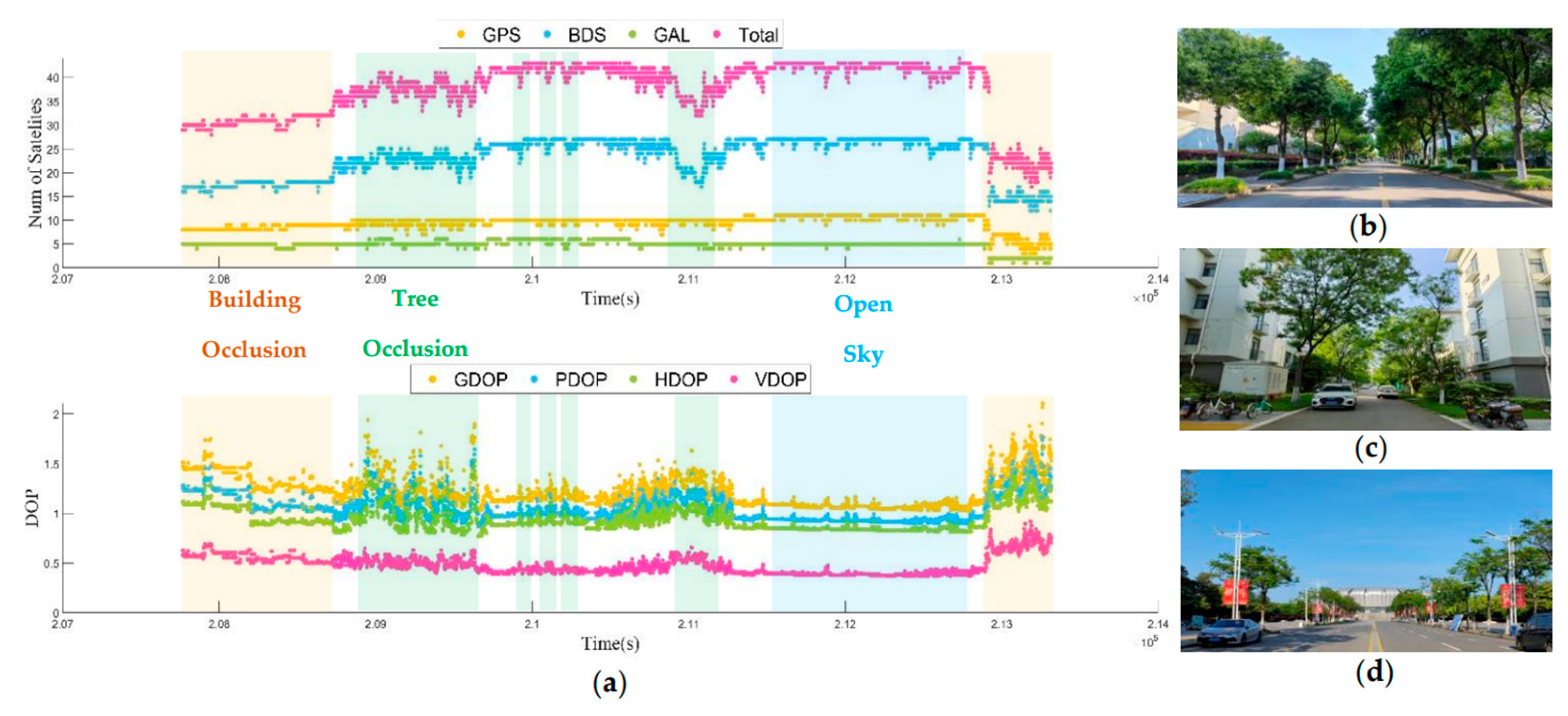
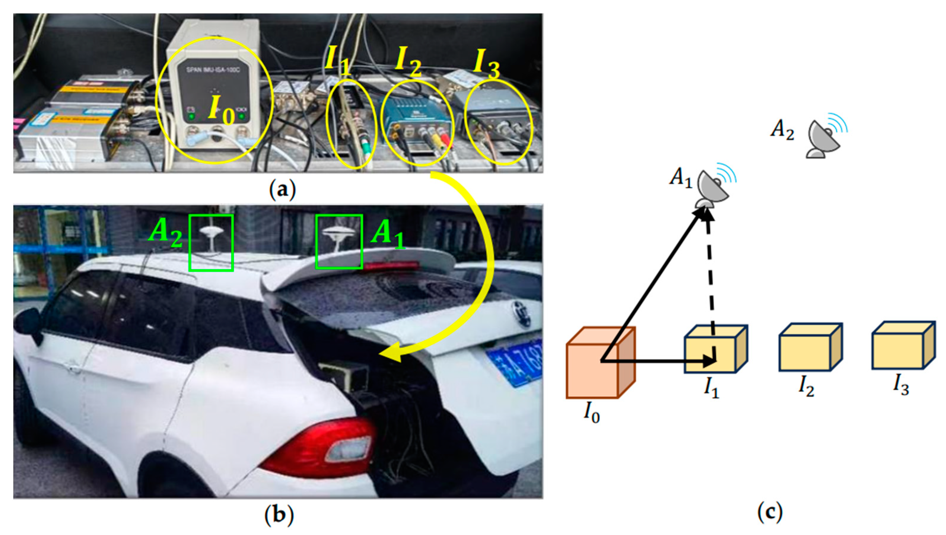
4.1.1. Equipment and Experiments of GNSS

As shown in Figure 4, the GNSS test equipment and trajectory are presented. During the test, the GNSS base station used was Unistrong, and the rover station used was Unicore 980, which is made by Unicore company, Beijing China; the reference benchmark utilized the NovAtelSpan100C integrated navigation system, and the collected integrated navigation data could be processed using forward and backward filtering in the IE (Inertial Explorer 8.9.6611) software platform to obtain the reference true value. The front antenna of the vehicle-mounted GNSS used the Survey Antenna PM100, while the rear antenna employed the multi-satellite and multi-frequency antenna SY-GNSS01, both installed on the roof of the test vehicle. After passing through the power divider, the received signal data were transmitted to the Unistrong 980 receiver and the NovAtelSpan100C receiver separately. Before the actual vehicle test, the lever arm vector between the inertial center of the NovAtelSpan100C and the GNSS rear antenna was measured to facilitate the conversion of the reference true value coordinates to the GNSS antenna center during post-processing.

As shown in Figure 5 below, during the data collection of the GNSS, the selected road sections include open sections, sections shaded by trees, sections blocked by buildings, etc.

• Under the open sky, the number and configuration of observable satellites vary. Obviously, in an open sky environment, the number of satellites from the three satellite systems remains relatively stable at each epoch, with the total number of available satellites maintained at around 35 to 40, and the DOP values also remain within a small range, with minimal fluctuations. Therefore, under an open sky environment, the satellite signal quality is high, and it is expected to produce stable and reliable GNSS positioning results.
• Under tree occlusion, the number of available satellites at each epoch decreases, and the total number of available satellites and DOP values fluctuate significantly, with some epochs even having GDOP values close to 2.0. Hence, in a shaded environment, the satellite signal is unstable, which may affect positioning accuracy.
• Under building occlusion, the number of satellites at each epoch decreases significantly. Unlike the shaded environment, in this scenario, the changes in the number of satellites and DOP values at each epoch fluctuate less. For this road section, it is necessary to find other positioning sources to compensate for positioning accuracy.

In summary, the satellite signal quality differs significantly under different sky conditions. To ensure the reliability of GNSS positioning results for subsequent multi-source fusion, it is necessary to evaluate the DOP values before the fusion process.

4.1.2. Equipment and Experiments of INS

Shown in Figure 6 is a schematic diagram of the INS test equipment and the installation lever arm. The INS data come from three integrated navigation devices: INS-D, Bynav, and NPOS. Since the test vehicle equipment includes roof antennas (primary $A_1$ and secondary $A_2$), satellite receivers, integrated navigation devices INS-D ($I_1$), Bynav ($I_2$), NPOS ($I_3$), and the high-precision integrated navigation device 100C ($I_0$), there is a lever arm effect during installation. For subsequent calculation experiments, the experimental data of INS-D will be used as an example, as the output data frequency of this device is 50 Hz.

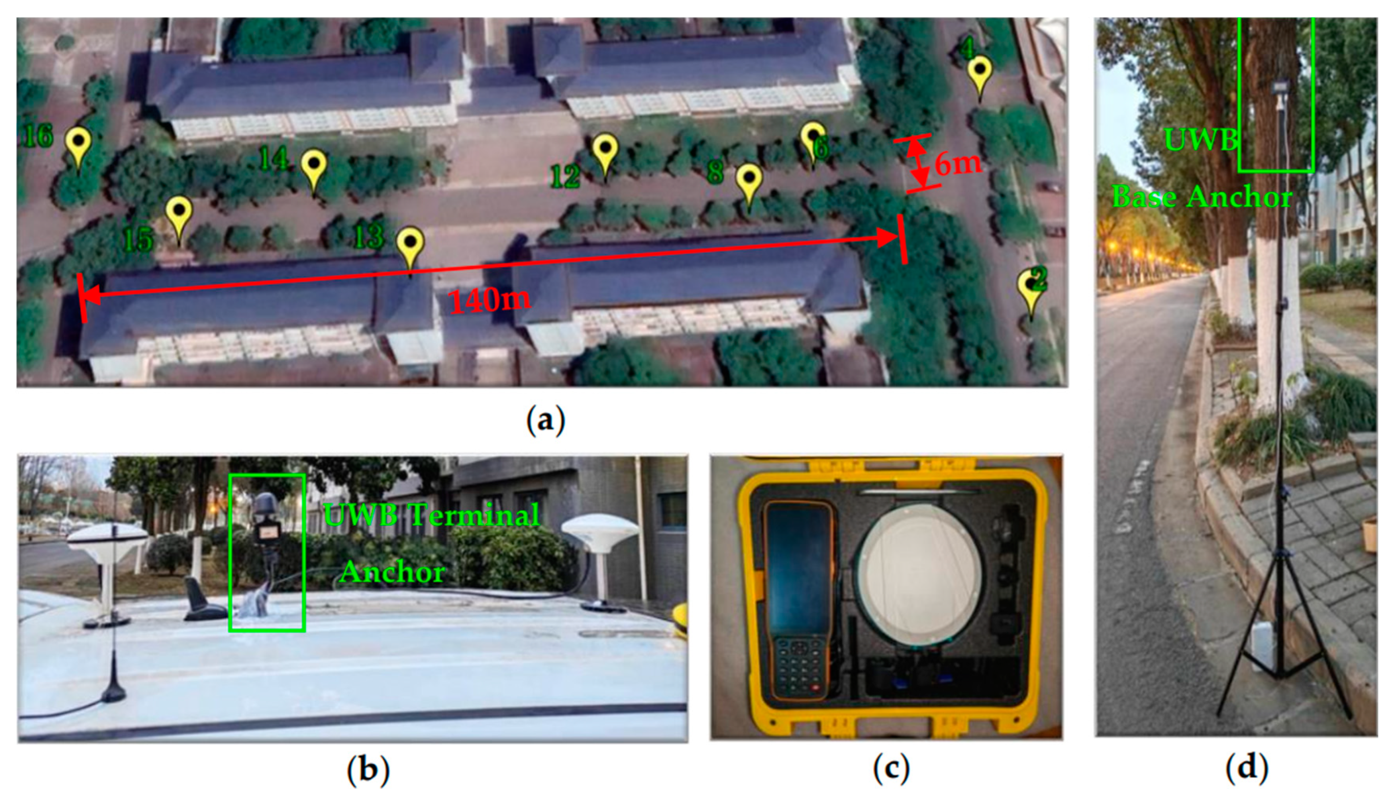
4.1.3. Equipment and Experiments of UWB

Figure 7 depicts the UWB test-related equipment and the distribution of base stations. To create a typical NLOS environment, this experiment was conducted in a dormitory area with high pedestrian traffic and cluttered with various objects. Nine UWB base stations were deployed on both sides of a road with a length of 140 m and a width of 6 m. These base stations were set at a consistent height, equivalent to the height of the UWB antenna mounted on the roof of the car. During the test, the nine base stations used the elongated antenna LinkTrack PS-B (with corresponding labels 2, 4, 6, 8, 12, 13, 14, 15, 16), and the positioning terminal tags used were LinkTrack P-BC. The ranging frequency was set at 50 Hz, and a CTI RTK instrument was used beforehand to perform high-precision positioning for each UWB base station.

To verify the rationality of the above UWB deployment configuration, as shown in Figure 8, is a GDOP value distribution map of the UWB test section. In this long and narrow section, limited by the number of UWB base stations and the deployment site, after comprehensive consideration of various factors, the above nine UWB base stations were finally deployed according to the triangular model, as much as possible. In this test section, the GDOP values formed by the nine base stations are mostly around 1.0, and the extreme values of GDOP often appear on the two shorter sides of the triangular model of the base stations, with their extreme values basically around 1.5. Overall, within the envelope space of the nine base stations mentioned above, the GDOP values are all less than 2.0, which meets the basic requirements for UWB positioning. However, outside the envelope space of the base stations, there are GDOP values greater than 2.0, even close to 3.0. Therefore, in the subsequent multi-source fusion system, it should be judged whether the current GDOP meets the requirements before updating the UWB measurements.

4.2. Results and Analysis

This article verifies the robustness and continuity of the GNSS/UWB/INS positioning system based on semi-tightly integrated robust estimation through post-processing. Based on the aforementioned theoretical research and experimental data collection, we compare the robust effects of the INS on GNSS and UWB positioning in semi-tightly integrated systems, as well as the advantages of multi-source integrated navigation in achieving continuous positioning under complex environments. In

Table 1. Statistical accuracy comparison of different models.

RMS	GNSS 1	GNSS/INS LC Robust	GNSS/INS STC Robust	UWB 2	UWB/INS LC Robust	UWB/INS STC Robust	GNSS/UWB/INS STC Robust
E/m	2.94	1.51	0.95	1.69	0.83	0.33	0.42
N/m	2.26	1.30	0.70	1.66	0.61	0.40	0.55
U/m	5.64	4.44	3.21	--	--	--	3.20

¹ The GNSSs mentioned in this table all refer to the RTD algorithm. ² The UWBs involved in this table all refer to two-dimensional plane positioning.

below, a comparison of positioning accuracy between the proposed semi-tightly integrated robust model and the traditional loosely integrated model on the test road section is presented:

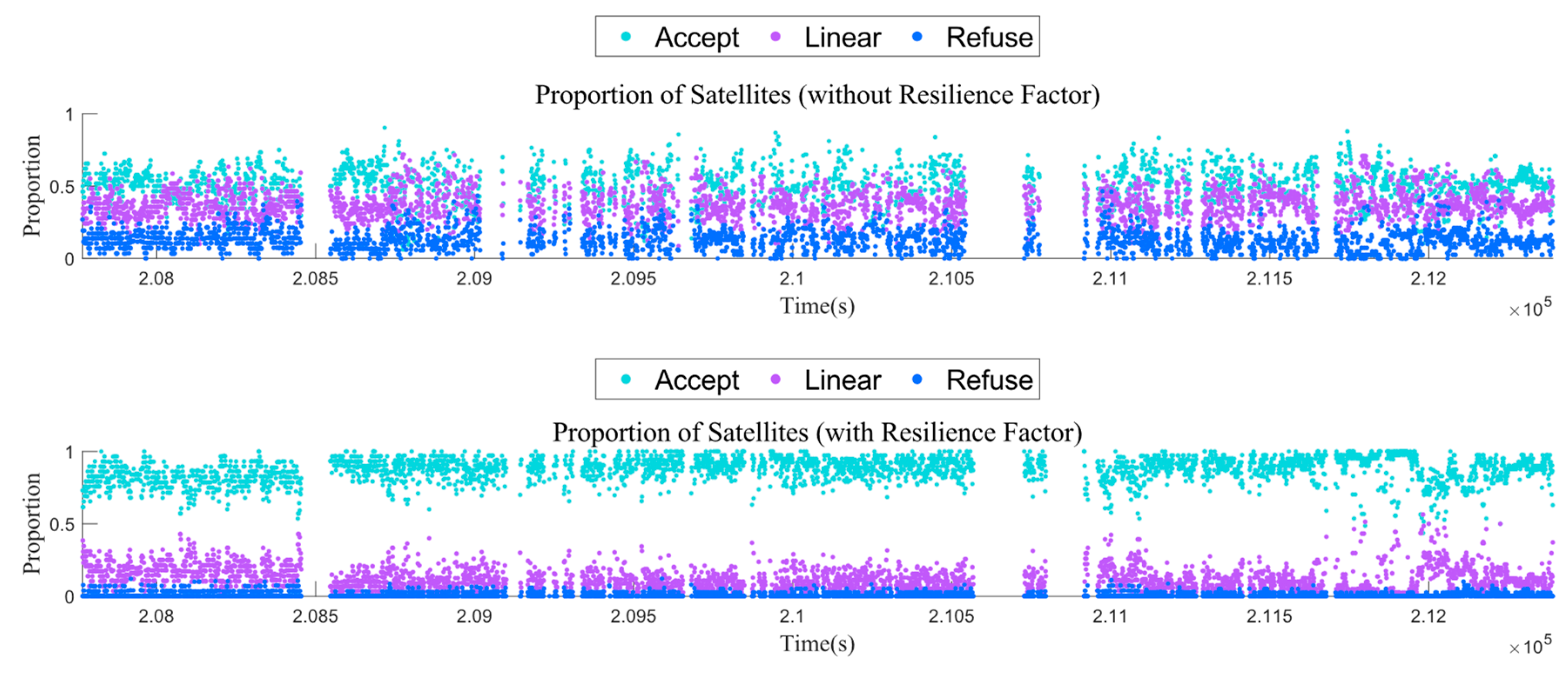
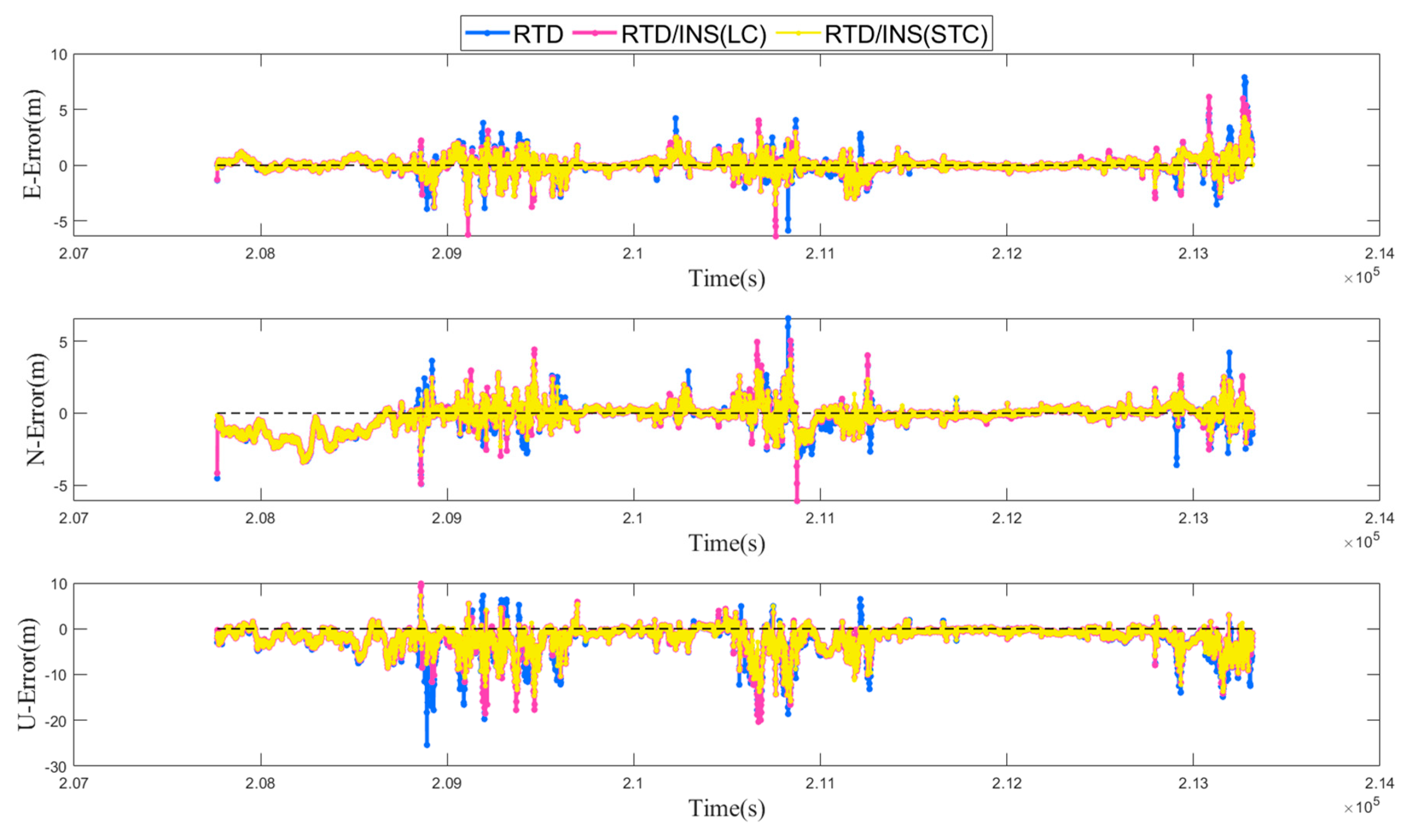
4.2.1. STC Robust Performance of GNSS/INS

Figure 9 depicts the error sequence of the GNSS/INS semi-tightly integrated positioning and RTD algorithm for GNSS positioning on the road segment shown in Figure 2. Additionally, a comparison is made with the error sequence of the GNSS single-positioning-source robust estimation, covering a duration of 92.5 min.

With the assistance of the INS, gross errors beyond 3 m can be stably identified, improving the reliability of positioning and enhancing the continuity of positioning to a certain extent. Similarly, the INS accumulates errors of nearly 1 s before updating GNSS measurements, and the accuracy of the introduced position information $x_{ins}, y_{ins},z_{ins}$ is between 1 m and 2 m. Therefore, the error range identified during pseudorange gross error detection should also be in the meter range, and there is no direct contribution to gross errors outside the accuracy range of INS dead reckoning results. The significance of introducing INS position domain information here is to ensure that the accuracy of the integrated navigation system remains stable within the accuracy range of system state prediction. This fusion strategy not only reduces the impact of gross errors on the GNSS measurements but also ensures the stability and reliability of the INS recursive main line.

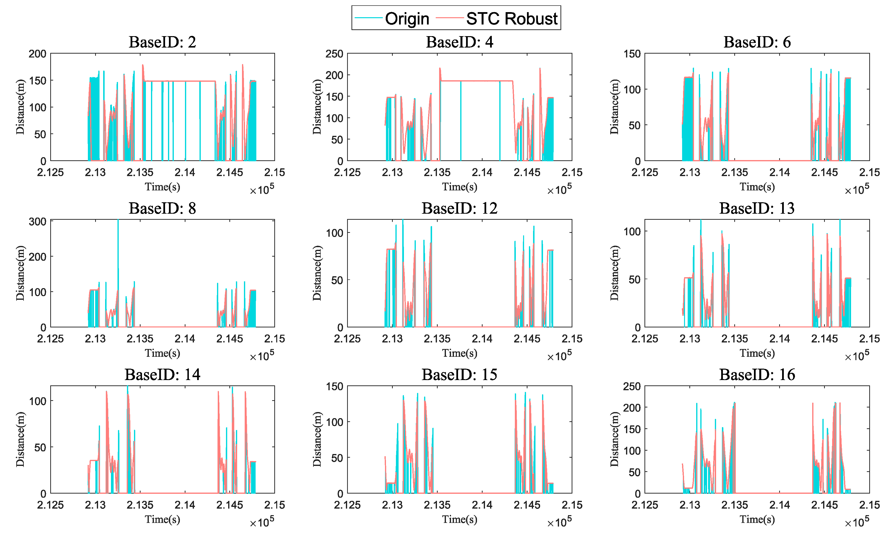
4.2.2. STC Robust Performance of UWB/INS

Figure 10 depicts the positioning error sequences in the E and N planes of the UWB/INS semi-tightly integrated positioning and the UWB single positioning source on the road segment where UWB base stations are deployed. Additionally, a comparison is made with the error sequence of the UWB/INS loosely integrated system. The duration of the test on this road segment is 340 s.

The road segment experienced three scenarios in total: a normal UWB signal area, a UWB signal blind area, and a UWB/INS integrated navigation recovery area:

• First, the normal zone. The positioning error of the UWB/INS semi-tightly integrated system is stably smaller than that of the loosely integrated system, while the UWB single positioning source often exhibits meter-level positioning jumps in this area.
• Second, the signal dead zone. Due to the insufficient number of available base stations, positioning cannot be achieved solely relying on UWB, while the INS can provide inertial dead reckoning. Therefore, in the green region of the graph, UWB/INS integrated positioning does not experience interruption until the UWB signal recovers after 85 s, during which time the integrated navigation system accumulates a total drift error of 20 m.
• Third, the recovery zone. The INS drift error is corrected under the measurement update of the UWB, allowing the filter’s state to gradually return to normal accuracy. It is worth noting that, since the semi-tightly integrated system provides INS position domain information, it prevents excessive elimination from causing UWB positioning failures. Therefore, under the semi-tightly integrated structure, the INS enters the drift state later, which in a sense verifies the role and effectiveness of tightly integrated navigation in maintaining positioning continuity.

4.2.3. STC Performance of GNSS/UWB/INS Integrated System

As shown in Figure 11, a comparison of the error sequences for GNSS/INS integrated positioning, UWB/INS integrated positioning, and GNSS/UWB/INS integrated positioning is presented for the road segment with UWB base stations deployed. This road segment has a complex sky environment with many ground disturbances, and the duration of the test is 340 s.

Similarly, the road segment can be divided into two scenarios: a UWB signal normal reception area and a UWB signal blind area:

• Firstly, the UWB signal normal zone. Due to severe building obstruction of the sky, the positioning accuracy of UWB/INS is significantly higher than that of GNSS/INS. Therefore, compared to GNSS/INS, the combined positioning accuracy of GNSS/UWB/INS is greatly improved.
• Secondly, the UWB signal dead zone. UWB cannot provide positioning, but relying on the positioning results of the GNSS, the combined navigation system can still achieve stable and continuous output. At this time, the positioning error of GNSS/UWB/INS is basically the same as that of GNSS/INS.
• Therefore, compared to the GNSS/INS and UWB/INS combined systems, the GNSS/UWB/INS positioning system designed in this paper can cope with dynamic and variable environments, achieving continuous and reliable positioning in challenging environments with both sky and ground obstructions.

As shown in Figure 12 below, a comparison of the positioning trajectories of GNSS/INS and GNSS/UWB/INS reveals that in the road segment with UWB base stations deployed, the positioning trajectory of GNSS/UWB/INS is more aligned with the true value. However, in the UWB signal blind area, the positioning trajectories of GNSS/UWB/INS and GINS largely overlap. This further verifies the superiority of this combined model in practical positioning applications.

5. Discussion

Based on the experimental results, the proposed semi-tightly coupled robust estimation method for GNSS/UWB/INS has played a significant role in quality control, mainly reflected in three aspects: identifying gross errors in observational data, suppressing the impact of gross errors on the estimator, and ensuring continuous and reliable results from the integrated positioning.

• Firstly, in terms of identifying gross errors, refer to Section 3.3 and Section 3.4. Due to the introduction of INS position domain information, it provides an a priori reference for the smaller-dimensional observations in challenging environments, enabling the identification of unacceptable gross errors within the accuracy range of the INS without causing systematic bias. Compared to the loosely coupled robust methods of similar complexity, this is a remarkable improvement.
• Secondly, in terms of suppressing gross errors, refer to Section 3.3.4 and Section 3.4.3. This paper, considering the differences in observation characteristics between the GNSS and UWB, employs the IGG III weighting degradation method based on resilience factors for GNSS pseudorange gross errors, and a threshold elimination method for UWB ranging NLOS gross errors. This can minimize the impact of gross errors on the system, while reducing information loss as much as possible.
• Finally, in terms of continuous and reliable positioning, refer to Section 4.2.3. This paper focuses on the challenges of reliability in complex sky–ground environments for GNSS and UWB positioning. A fusion framework based on DOP value judgments is proposed, which can achieve a complementary accuracy between the GNSS and UWB in dynamic and changing environments, while ensuring reliable positioning results.

6. Conclusions

In summary, this paper proposes a GNSS/UWB/INS integrated navigation and positioning method based on a semi-tightly coupled robust model. It fully utilizes the position domain information of the INS to provide an a priori reference for the robustness of the original measurement data from the GNSS and UWB, especially in complex sky and ground environments. When the number of available satellites and UWB base stations is insufficient to easily identify the overall offset of system errors, this semi-tightly coupled structure can ensure that the positioning system does not experience unexpected jumps. Additionally, this paper fully considers the differences in the number of observations between the GNSS and UWB and employs different methods when introducing the positional constraints of the INS. Experimental results demonstrate that, compared to the internal robustness of a single positioning source and loosely coupled robustness, the proposed semi-tightly coupled robust method makes the positioning structure more reliable and smooth, enabling reliable and continuous positioning in complex and variable scenarios.

However, due to limitations in testing conditions, this study has two limitations. Firstly, GNSS positioning only considers inter-satellite differential positioning algorithms. Secondly, UWB only achieves two-dimensional planar positioning. Future work will improve the testing experiments and thoroughly investigate the advantages of this semi-tightly coupled structure under different algorithms.

References

1. Yang, Y.; Ren, X.; Jia, X. Development trends of the national secure PNT system based on BDS. Sci. China Earth Sci. 2023, 66, 929–938. [Google Scholar] [CrossRef]
2. Prol, F.S.; Ferre, R.M.; Saleem, Z. Position, navigation, and timing (PNT) through low earth orbit (LEO) satellites: A survey on current status, challenges, and opportunities. IEEE Access 2022, 10, 83971–84002. [Google Scholar] [CrossRef]
3. Wang, J.; Chen, X.; Shi, C. Robust M-estimation-Based ICKF for GNSS Outlier Mitigation in GNSS/SINS navigation applications. IEEE Trans. Instrum. Meas. 2023, 72, 8505617. [Google Scholar] [CrossRef]
4. Zhang, B.; Hou, P.; Zha, J. PPP–RTK functional models formulated with undifferenced and uncombined GNSS observations. Satell. Navig. 2022, 3, 3. [Google Scholar] [CrossRef]
5. Zhang, B.; Zhao, C.; Odolinski, R. Functional model modification of precise point positioning considering the time-varying code biases of a receiver. Satell. Navig. 2021, 2, 1–10. [Google Scholar] [CrossRef]
6. Feng, X.; Zhang, T.; Lin, T. Implementation and performance of a deeply-coupled GNSS receiver with low-cost MEMS inertial sensors for vehicle urban navigation. Sensors 2020, 20, 3397. [Google Scholar] [CrossRef] [PubMed]
7. Zhu, J.; Zhou, H.; Wang, Z. Improved Multi-sensor Fusion Positioning System Based on GNSS/LiDAR/Vision/IMU with Semi-tightly Coupling and Graph Optimization in GNSS Challenging Environments. IEEE Access 2023, 11, 95711–95723. [Google Scholar] [CrossRef]
8. Chen, Q.; Zhang, Q.; Niu, X. Estimate the pitch and heading mounting angles of the IMU for land vehicular GNSS/INS integrated system. IEEE Trans. Intell. Transp. Syst. 2020, 22, 6503–6515. [Google Scholar] [CrossRef]
9. Jang, B.J. Principles and trends of UWB positioning technology. J. Korean Inst. Electromagn. Eng. Sci. 2022, 33, 1–11. [Google Scholar] [CrossRef]
10. Brovko, T.; Chugunov, A.; Malyshev, A. Complex Kalman filter algorithm for smartphone-based indoor UWB/INS navigation systems. In Proceedings of the Ural Symposium on Biomedical Engineering, Radioelectronics and Information Technology (USBEREIT), Yekaterinburg, Russia, 13–14 May 2021; pp. 0280–0284. [Google Scholar]
11. Wang, C.; Xu, A.; Sui, X.; Hao, Y.; Shi, Z.; Chen, Z. A seamless navigation system and applications for autonomous vehicles using a tightly coupled GNSS/UWB/INS/map integration scheme. Remote Sens. 2021, 14, 27. [Google Scholar] [CrossRef]
12. Ren, Z.; Liu, S.; Dai, J. Research on Kinematic and Static Filtering of the ESKF Based on INS/GNSS/UWB. Sensors 2023, 23, 4735. [Google Scholar] [CrossRef]
13. Yao, L.; Li, M.; Xu, T. GNSS/UWB/INS indoor and outdoor seamless positioning algorithm based on federal filtering. Meas. Sci. Technol. 2023, 35, 015135. [Google Scholar] [CrossRef]
14. Boguspayev, N.; Akhmedov, D.; Raskaliyev, A. A comprehensive review of GNSS/INS integration techniques for land and air vehicle applications. Appl. Sci. 2023, 13, 4819. [Google Scholar] [CrossRef]
15. Li, S.; Wang, S.; Zhou, Y. Tightly coupled integration of GNSS, INS, and LiDAR for vehicle navigation in urban environments. IEEE Internet Things J. 2022, 9, 24721–24735. [Google Scholar] [CrossRef]
16. Falco, G.; Pini, M.; Marucco, G. Loose and tight GNSS/INS integrations: Comparison of performance assessed in real urban scenarios. Sensors 2017, 17, 255. [Google Scholar] [CrossRef] [PubMed]
17. Lou, T.S.; Chen, N.H.; Chen, Z.W. Robust partially strong tracking extended consider Kalman filtering for INS/GNSS integrated navigation. IEEE Access 2019, 7, 151230–151238. [Google Scholar] [CrossRef]
18. Li, T.; Zhang, H.; Niu, X.; Gao, Z. Tightly-coupled integration of multi-GNSS single-frequency RTK and MEMS-IMU for enhanced positioning performance. Sensors 2017, 17, 2462. [Google Scholar] [CrossRef]
19. Jiang, Y.; Pan, S.; Meng, Q. Performance Analysis of Robust Tightly Coupled GNSS/INS Integration Positioning Based on M Estimation in Challenging Environments. In China Satellite Navigation Conference; Springer Nature: Singapore, 2022; pp. 400–414. [Google Scholar]
20. Wang, D.; Dong, Y.; Li, Z. Constrained MEMS-based GNSS/INS tightly coupled system with robust Kalman filter for accurate land vehicular navigation. IEEE Trans. Instrum. Meas. 2019, 69, 5138–5148. [Google Scholar] [CrossRef]
21. Li, X.; Wang, X.; Liao, J. Semi-tightly coupled integration of multi-GNSS PPP and S-VINS for precise positioning in GNSS-challenged environments. Satell. Navig. 2021, 2, 1. [Google Scholar] [CrossRef]
22. Ma, C.; Pan, S.; Gao, W. Variational Bayesian-based robust adaptive filtering for GNSS/INS tightly coupled positioning in urban environments. Measurement 2023, 223, 113668. [Google Scholar] [CrossRef]
23. Yang, B.; Li, J.; Shao, Z. Robust UWB indoor localization for NLOS scenes via learning spatial-temporal features. IEEE Sens. J. 2022, 22, 7990–8000. [Google Scholar] [CrossRef]
24. Pan, S.; Meng, X.; Gao, W. A new approach for optimising GNSS positioning performance in harsh observation environments. J. Navigat. 2014; 67, 1029–1048. [Google Scholar]
25. Zaman, B.; Mahfooz, S.Z.; Mehmood, R. An adaptive EWMA control chart based on Hampel function to monitor the process location parameter. Qual. Reliab. Eng. Int. 2023, 39, 1277–1298. [Google Scholar] [CrossRef]
26. Sinova, B.; Van Aelst, S. Advantages of M-estimators of location for fuzzy numbers based on Tukey’s biweight loss function. Int. J. Approx. Reason. 2018, 93, 219–237. [Google Scholar] [CrossRef]
27. Huber, P.; Peter, J. Robust estimation of a location parameter. Ann. Math. Stat. 1964, 35, 73–101. [Google Scholar] [CrossRef]
28. Yang, Y.; Gao, W.; Zhang, X. Robust Kalman filtering with constraints: A case study for integrated navigation. J. Geod. 2010, 84, 373–381. [Google Scholar] [CrossRef]
29. Amami, M.M. The Advantages and Limitations of Low-Cost Single Frequency GPS/MEMS-Based INS Integration. Glob. J. Eng. Technol. Adv. 2022, 10, 018–031. [Google Scholar] [CrossRef]
30. Fredeluces, E.; Ozeki, T.; Kubo, N. Modified RTK-GNSS for Challenging Environments. Sensors 2024, 24, 2712. [Google Scholar] [CrossRef] [PubMed]
31. Su, M.; Chang, X.; Zheng, F. Theory and Experiment Analysis on the Influence of Floods on a GNSS Pseudo-Range Multipath and CNR Signal Based on Two Cases Study in China. Remote Sens. 2022, 14, 5874. [Google Scholar] [CrossRef]
32. Xue, A.; Kong, H.; Lao, Y. A new robust identification method for transmission line parameters based on ADALINE and IGG Method. IEEE Access 2020, 8, 132960–132969. [Google Scholar] [CrossRef]
33. Zhang, Z.; Li, X.; Yuan, H. An enhanced outlier processing approach based on the resilient mathematical model compensation in GNSS precise positioning and navigation. Meas. Sci. Technol. 2023, 35, 015007. [Google Scholar] [CrossRef]
34. Zhang, H.; Li, Z.; Zheng, S. UWB/INS-based robust anchor-free relative positioning scheme for UGVs. Meas. Sci. Technol. 2022, 33, 125007. [Google Scholar] [CrossRef]
35. Won, D.H.; Lee, E.; Heo, M. Selective integration of GNSS, vision sensor, and INS using weighted DOP under GNSS-challenged environments. IEEE Trans. Instrum. Meas. 2014, 63, 2288–2298. [Google Scholar] [CrossRef]
36. Wang, H.S.; Kao, A. A behavioral approach to GNSS positioning and DOP determination. WSEAS Trans. Syst. 2008, 7, 854–869. [Google Scholar]
37. Tahsin, M.; Sultana, S.; Reza, T. Analysis of DOP and its preciseness in GNSS position estimation. In Proceedings of the 2015 International Conference on Electrical Engineering and Information Communication Technology (ICEEICT), Savar, Bangladesh, 21–23 May 2015; pp. 1–6. [Google Scholar]
38. Feng, G.; Shen, C.; Long, C. GDOP index in UWB indoor location system experiment. In Proceedings of the 2015 IEEE SENSORS, Busan, Republic of Korea, 1–4 November 2015; pp. 1–4. [Google Scholar]
Figure 1. Semi-tightly coupled robust model for GNSS/UWB/INS integrated system.
Remotesensing 16 02108 g001
Figure 2. The proportion of three-stage satellites with the resilience factor.
Remotesensing 16 02108 g002
Figure 3. The distance measurement of each UWB base with STC Robust.
Remotesensing 16 02108 g003
Figure 4. Equipment for GNSS and tracks of experiment. (a) Dynamic vehicle. (b) Unistrong980. (c) NovAtelSpan100C. (d) Experimental trajectory.
Remotesensing 16 02108 g004
Figure 5. Environments of GNSS experiment and satellite conditions. (a) Satellite conditions. (b) Tree occlusion. (c) Building occlusion. (d) Open sky.
Remotesensing 16 02108 g005
Figure 6. Equipment for INS and lever arm of installation. (a) INS equipment. (b) Dynamic vehicle. (c) Lever arm of installation.
Remotesensing 16 02108 g006
Figure 7. Equipment for UWB and the distribution of base anchors. (a) Distribution of UWB base anchors. (b) Experimental antenna. (c) CTI RTK instrument. (d) UWB base anchor.
Remotesensing 16 02108 g007
Figure 8. GDOP value distribution of UWB base station.
Remotesensing 16 02108 g008
Figure 9. GNSS/INS positioning error sequence comparison.
Remotesensing 16 02108 g009
Figure 10. UWB/INS positioning error sequence comparison.
Remotesensing 16 02108 g010
Figure 11. GNSS/UWB/INS positioning error sequence comparison.
Remotesensing 16 02108 g011
Figure 12. GNSS/UWB/INS positioning tracks comparison.
Remotesensing 16 02108 g012