Analyzing Spatial–Temporal Characteristics and Influencing Mechanisms of Landscape Changes in the Context of Comprehensive Urban Expansion Using Remote Sensing

Abstract

The phenomena of global climate change and comprehensive urban expansion have precipitated significant and unprecedented transformations in landscape patterns. To enhance the assessment of these spatio−temporal changes and their driving forces at a regional level, we developed a comprehensive landscape index (CLI) to quantify these patterns and conducted a detailed analysis of the spatio−temporal variations in Minnesota over the last two decades. Our analysis of the CLI was conducted by examining both its quantitative relationships and spatial distribution patterns. The findings indicate a consistent increase in Minnesota’s CLI over this period, marked by an escalation in landscape fragmentation and diversity, alongside a decline in landscape connectivity. Temporally, the CLI experienced a notable shift in 2010. Spatially, the clustering characteristics of landscape patterns have largely remained stable. Our analysis reveals that the CLI is most sensitive to total population (POP) and gross domestic product (GDP) factors, underscoring the significant impact of human activity on landscape patterns. Notably, the explanatory capacity of interactions between factors is substantially greater than that of individual factors, with the GDP and vegetation structure (VS) interaction demonstrating the greatest influence on the spatial distribution of landscape patterns. This highlights the critical role of the interplay between human socio−economic activity and vegetation coverage in shaping landscape configurations.

1. Introduction

The rapid advancement of socio−economic development and urban sprawl has expedited the transition among various land use categories, precipitating alterations in regional landscape configurations [1,2]. During urban expansion phases, extensive tracts of natural landscapes, agricultural lands, and forests are invariably converted into urban built environments [3,4,5,6]. Such transformations engender increased fragmentation of the erstwhile cohesive landscape patterns [7,8], resulting in the subdivision of large, natural expanses into numerous smaller segments. This process not only elevates the quantity and density of landscape patches but also augments the complexity of landscape patterns [9,10,11]. Concurrently, modifications in landscape patterns bear significant implications for regional ecosystems [12,13,14]. The encroachment of urban development can disrupt established ecological corridors, thereby impairing biodiversity and ecosystem equilibrium, which, in turn, poses challenges to the sustainable development of urban areas [15]. Hence, elucidating the spatio−temporal dynamics of landscape patterns alongside their underlying drivers holds paramount importance for informed landscape planning and management, as well as fostering urban sustainability. This study considers the effects of comprehensive urban expansion on landscape pattern, including artificial surface physical expansion, population spread, and GDP growth. In this vein, Minnesota, with its diverse land use types and distinctive landscape patterns, presents an illustrative case study. The state boasts extensive agricultural lands and forested areas characterized by robust connectivity [16,17], juxtaposed against a fragmented landscape dissected by a dense network of water bodies [18]. However, the rapid pace of urbanization and urban sprawl over recent decades has placed the landscape patterns and ecological integrity of Minnesota under considerable strain.

Landscape pattern represents a multifaceted reflection of spatial heterogeneity within landscapes, characterized by the distribution and arrangement of patches varying in size, shape, and attributes across geographical spaces [19]. It encapsulates the outcomes of both natural and anthropogenic influences over time and space [20,21,22]. Alterations in landscape patterns at a regional level are pivotal, impacting ecological security [23,24], promoting sustainable development [25,26], and serving as a crucial metric of the interplay between socio-economic systems and natural ecosystems [27,28]. A suite of landscape metrics, including the total number of patches, patch density, aggregation index, separation index, and landscape diversity index, among others [28,29,30,31,32], are extensively employed for the analysis, monitoring, and planning of landscape patterns. These indices facilitate the quantification of landscape spatial structures, offering insights into landscape scale, spatial clustering, connectivity, and diversity. The landscape index emerges as a vital tool in examining land use transformations and landscape spatial configurations amidst urban expansion. Zhang et al., found that the patch density and shape complexity, landscape diversity, and fragmentation of the landscape continued to increase while landscape connectivity declined in the process of urbanization [31]. Kennedy et al. extracted the landscape index by Fragstats 4.2 and found that unprecedented landscape fragmentation occurred in Koitobos river sub-basin, Trans-Nzoia, Kenya [33]. Traditional landscape metrics, however, are often constrained to singular indices that address specific landscape issues in isolation, with prevailing research predominantly focusing on the sequential analysis of individual characteristics before qualitatively integrating these observations to depict the overall landscape [29,34,35]. This fragmented approach hampers the quantitative assessment of a region’s comprehensive landscape. Researchers have attempted to integrate multiple landscape indices. Zhang et al. constructed an integrated spatial landscape index (ISLI) [36]. Guan et al. proposed a comprehensive landscape sensitivity index (CLSI) based on landscape and urban development [37]. Therefore, this study amalgamates multiple landscape metrics into a unified comprehensive landscape index (CLI), enabling a systematic analysis of the spatial structure and spatiotemporal dynamics of the landscape.

Research on landscape patterns predominantly concentrates on the temporal and spatial dynamics within specific regions [38,39,40] and the determinants driving these changes amidst urban expansion [29,41,42,43,44]. However, regarding the temporal scope, prior studies have typically focused on brief periods [39] or selected years within longer intervals [29,43,44]. Yet, the evolution of landscape patterns in a region is a protracted process, influenced by sustained human activity, significant infrastructural development, and natural disasters [45]. The conventional practice of selecting temporal nodes at regular intervals may inadvertently overlook critical human or natural events, underscoring the necessity for continuous, long-term investigation in this domain. As a reliable, dynamic, and high-quality data source, remote sensing data has the characteristics of large amounts of information and long-term continuity compared with traditional data [46]. Therefore, various types of remote sensing data are widely used in the study of urban problems [47,48]. Since remote sensing data can provide continuous land cover/use data, a large number of studies have been conducted to analyze urban landscape change based on remote sensing data [42,49,50,51]. In this study, landscape index and its driving factors were extracted from multi-source remote sensing data to help realize long-term and large-scale landscape pattern research.

The phenomenon of rapid urban expansion has led to increasingly complex changes in landscape patterns, transforming singular, continuous natural areas into heterogeneous, discontinuous patches [52,53]. While measuring landscape patterns and their alterations provides a superficial understanding of land cover composition and spatial characteristics, it falls short of fulfilling the requirements for a profound comprehension of landscape evolution and the necessities of regional landscape management and planning [54]. Consequently, it is imperative to elucidate the reasons behind landscape pattern evolution and to quantify the extent and manner in which each driving factor influences these patterns. Guo et al. used redundancy and grey correlation analysis to study the driving factors of landscape pattern [55]. Yang et al., detected that socio-economic factors are the most important factors in landscape pattern transformation using principal component analysis [56]. Although most existing research focuses on the quantitative relationships between driving factors and landscape patterns [56,57,58,59], analyzing the influence mechanisms of various drivers, they often overlook the spatial impact these factors have on the driving mechanisms of landscape patterns. Given the complex spatial heterogeneity inherent in natural and social systems, drivers exert differing effects on landscape patterns depending on their geographical locations [43,60]. Wu et al. found that the distribution of each landscape index had obvious spatial differentiation [61]. Thus, accounting for the spatial heterogeneity of driving mechanisms is crucial for a more accurate depiction of these mechanisms across diverse geographical contexts. This study quantitatively analyzes the influencing mechanisms while considering their spatial patterns and heterogeneity. Evidence suggests that both natural factors and human activity are significant in shaping landscapes [62,63], with natural factors such as terrain and landform directly influencing landscape formation and evolution, and human activity altering landscapes through land use and transformation. However, the impact of these two factor types on landscape patterns is not isolated; rather, they interact synergistically. Wu et al., found that there was a significant interaction enhancement effect between natural and social factors in influencing landscape fragmentation [61]. Nie et al., found the digital elevation model (DEM) and GDP to be the main drivers of landscape patterns using Geodetectors [8]. Therefore, in contrast to studies focusing solely on the influence of individual factors [64,65], research into the combined contributions of population, economic, and natural interactions to landscape patterns merits greater attention [66,67].

The principal contributions of this study, as distinguished from previous research, are multifaceted and can be delineated as follows: (1) comprehensive landscape index construction: Utilizing multiple landscape metrics, this study develops a comprehensive landscape index. This innovation facilitates a simplified quantitative interpretation of regional-scale comprehensive landscape characteristics, which surpasses the capabilities of traditional indicators. (2) Spatio-temporal analysis: A systematic examination of the spatio-temporal evolution of landscape patterns is conducted, integrating both temporal and spatial dimensions. This approach provides a holistic understanding of landscape dynamics over time and across space. (3) Exploration of influence mechanisms considering spatial heterogeneity: By focusing on spatial heterogeneity, this study delves into the mechanisms influencing landscape patterns. It evaluates the effects of both individual drivers and the combined impact of multiple factors, offering insights into their complex interplay. (4) Comprehensive quantification using remote sensing data: Leveraging the temporal continuity and spatial resolution of remote sensing data, this research achieves a comprehensive quantification of its objectives. This includes identifying landscape characteristics, investigating the temporal trends and spatial distribution of landscape patterns, and analyzing the driving factors behind these patterns. Collectively, these contributions underscore the study’s innovative approach to understanding landscape patterns, offering valuable perspectives for regional landscape management and planning.

2. Materials and Methods

2.1. Study Area

Spanning latitudes from 43°30′N to 49°23′N and longitudes from 89°29′W to 97°14′W, Minnesota, located in the Midwest of the United States, shares its borders with Canada to the north, Lake Superior to the east, Iowa to the south, and both South and North Dakota to the west. Minnesota has a temperate continental climate. There are four distinct seasons, with cold winters averaging −2 °C in January and hot summers averaging 25 °C in July [68]. Average annual precipitation ranges from 510 mm in the northwest to about 890 mm in the southeast [69]. The state is administratively divided into 87 counties, covering a total area of 219,000 square kilometers (Figure 1). Characterized by its diverse land types and complex landscape patterns, Minnesota encompasses four principal ecological regions (biomes) of North America: aspen parklands, prairie grasslands, deciduous forests, and coniferous forests, thereby enriching its land-type variety. The state’s intricate surface-water system and abundant inland lakes contribute to a mosaic of land patches, engendering a unique and complex landscape pattern. Nonetheless, Minnesota’s urban population continues to grow, with more than 80% of Minnesota residents living in an urban area [70]. From 1975 to 2006, the urban area of the Twin Cities of Minnesota grew at an average rate of more than 4000 ha per year, and this trend is expected to continue [71]. The rapid expansion of artificial surfaces has precipitated significant alterations in Minnesota’s surface structure. These ecological regions are currently confronting challenges such as reduction in patch sizes, landscape fragmentation, and biodiversity loss. Comprehensive urban expansion has notably led to the extensive conversion of Minnesota’s grasslands into agricultural lands, with the original 18 million acres of tallgrass prairie now diminished to less than 1% [72]. Concurrently, significant deforestation and fragmentation of forest landscapes have occurred [73], alongside a trend towards the consolidation of farmlands, reducing the number of farms but increasing their average size. Given these circumstances, it is imperative to select Minnesota as a focal area for investigating the impacts of comprehensive urban expansion on landscape pattern transformations.

2.2. Data and Resources

In this study, Minnesota was selected as the study area to explore the spatio-temporal characteristics of landscape patterns and their influencing mechanisms. Firstly, 10 selected landscape indices were utilized to construct a CLI using PCA to describe the spatial and temporal trends of landscape patterns from 1998 to 2018. Secondly, the Mann–Kendall trend test and the Pettitt test were utilized to test the temporal trend and mutation points, and spatial autocorrelation was utilized to reveal the clustering effect of urban landscape pattern. Thirdly, the Geodetector model was used to analyze the influencing mechanism of landscape pattern in Minnesota (Figure 2).

Integrating insights from both domestic and international research on landscape patterns, this study identifies key factors that influence land use and cover, including vegetation coverage (VS), artificial land coverage (AS), slope (SLP), total population (POP), and gross national product (GDP). The data sources are shown in

Table 1. Data and resources.

Name	Dataset	Spatial Resolution	Temporal Resolution
VS (vegetation coverage)	MCD12Q1.061 MODIS Land Cover Type Yearly Global	500 m	Yearly
AS (artificial land coverage)	USFS Landscape Change Monitoring System v2022.8	30 m	Yearly
SLP (slope)	Minnesota Geospatial Commons (https://gisdata.mn.gov/dataset/elev-30m-digital-elevation-model, accessed on 29 May 2024)	30 m	--
POP (total population)	United States Census Bureau (https://www.census.gov/quickfacts/, accessed on 29 May 2024)	--	Yearly
GDP (gross domestic product)	Minmesota Department of Employment and Economic Development (https://mn.gov/deed/data/economic-analysis/compare/compare-metro/economy/gdp.jsp, accessed on 29 May 2024)	--	Yearly

. These factors are pivotal in analyzing the driving mechanisms underlying landscape pattern changes. Land use and cover play a critical role in shaping landscape patterns on both global and regional scales [74,75]. Accordingly, VS and artificial AS were selected as primary indicators to represent land use and cover dynamics in this study. The slope of the land, as a fundamental aspect of land surface morphology, influences the structure of agricultural lands and urban patterns, thereby significantly affecting the regional landscape pattern [76]. Utilizing digital elevation model (DEM) data, this research calculates the SLP as a critical factor that encapsulates the terrain’s influence on landscape patterns. Furthermore, human activity, manifested through long-term productive endeavors, directly induce alterations in landscape structure, exhibiting a quantifiable relationship [77]. Hence, this study incorporates POP and the GDP as indicators to quantify human influence on landscape patterns.

The VS, AS, and SLP factors were derived from remote sensing images, and the POP and GDP factors are county-level panel data. In this paper, we used various remote sensing images. In order to ensure that the spatio-temporal resolution of each data point was consistent, we aggregated the VS, AS, and SLP factors to the county level. By combining raster data with vector data, the problem of different spatio-temporal resolutions of various remote sensing images was avoided.

2.3. Methodology

2.3.1. Landscape Indices

This study quantified an array of landscape indices at the landscape scale, encompassing the number of patches ($\mathrm{N}\mathrm{P}$), patch density ($\mathrm{P}\mathrm{D}$), largest patch index ($\mathrm{L}\mathrm{P}\mathrm{I}$), perimeter-area fractal dimension ($\mathrm{P}\mathrm{A}\mathrm{F}\mathrm{R}\mathrm{A}\mathrm{C}$), contagion index ($\mathrm{C}\mathrm{O}\mathrm{N}\mathrm{T}\mathrm{A}\mathrm{G}$), aggregation index ($\mathrm{A}\mathrm{I}$), splitting index ($\mathrm{S}\mathrm{P}\mathrm{L}\mathrm{I}\mathrm{T}$), patch cohesion index ($\mathrm{C}\mathrm{O}\mathrm{H}\mathrm{E}\mathrm{S}\mathrm{I}\mathrm{O}\mathrm{N}$), Shannon diversity index ($\mathrm{S}\mathrm{H}\mathrm{D}\mathrm{I}$), and Shannon evenness index ($\mathrm{S}\mathrm{H}\mathrm{E}\mathrm{I}$). Collectively, these ten indices encapsulate aspects such as the quantity, size, fragmentation, proximity, diversity, and cohesion of the landscape, thereby addressing broad landscape concerns. The specifics of each landscape index are delineated in

Table 2. Landscape metrics.

Landscape Metrics	Description	Formula
$\mathrm{N}\mathrm{P}$ (number of patches)	The number of patches describes the fragmentation of the landscape but does not necessarily contain information about the configuration or composition of the landscape.
$\mathrm{P}\mathrm{D}$ (patch density)	PD equals the number of patches of the corresponding patch type (NP) divided by the total landscape area.	$PD=NP/A$
$\mathrm{L}\mathrm{P}\mathrm{I}$ (largest patch index)	LPI equals the percentage of the landscape comprising the largest patch.	$LPI=\frac{a_{max}}{A}\times 100$
$\mathrm{P}\mathrm{A}\mathrm{F}\mathrm{R}\mathrm{A}\mathrm{C}$ (perimeter-area fractal dimension)	$\mathrm{P}\mathrm{A}\mathrm{F}\mathrm{R}\mathrm{A}\mathrm{C}$ describes the patch complexity of the landscape while being scale independent.	$PAFRAC=\frac{2}{\frac{N{\sum }_{i=1}^m{\sum }_{j=1}^n\left(ln{p}_{ij}\times ln{a}_{ij}\right)-{\sum }_{i=1}^m{\sum }_{j=1}^{n}ln{p}_{ij}\times {\sum }_{i=1}^m{\sum }_{j=1}^{n}ln{a}_{ij}}{N{\sum }_{i=1}^m{\sum }_{j=1}^{n}ln{p_{ij}}^2-{\sum }_{i=1}^m{\sum }_{j=1}^{n}ln{p}_{ij}}}$
$\mathrm{C}\mathrm{O}\mathrm{N}\mathrm{T}\mathrm{A}\mathrm{G}$ (contagion index)	$\mathrm{C}\mathrm{O}\mathrm{N}\mathrm{T}\mathrm{A}\mathrm{G}$ measures the degree of clumping of attributes on raster maps.	$CONTAG=\left[1+\frac{{\sum }_{i=1}^m{\sum }_{k=1}^m\left[P_i\times \left(\frac{g_{ik}}{{\sum }_{k=1}^m{g}_{ik}}\right)\right]\times \left[\mathit{ln}(P_i)\left(\frac{g_{ik}}{{\sum }_{k=1}^m{g}_{ik}}\right)\right]}{2\mathit{ln}\left(m\right)}\right]\times 100$
$\mathrm{A}\mathrm{I}$ (aggregation index)	AI measures the extent to which land cover patches of the same category are spatially connected or proximate to one another, relative to a maximally aggregated distribution of those patches.	$AI=\left[\frac{g_{ij}}{max\to g_{ij}}\right]\times 100$
$\mathrm{S}\mathrm{P}\mathrm{L}\mathrm{I}\mathrm{T}$ (splitting index)	$\mathrm{S}\mathrm{P}\mathrm{L}\mathrm{I}\mathrm{T}$ describes the number of patches if all the landscape were divided into equally sized patches.	$SPLIT=\frac{A^2}{{\sum }_{j=1}^n{a_{ij}}^2}$
$\mathrm{C}\mathrm{O}\mathrm{H}\mathrm{E}\mathrm{S}\mathrm{I}\mathrm{O}\mathrm{N}$ (patch cohesion index)	$\mathrm{C}\mathrm{O}\mathrm{H}\mathrm{E}\mathrm{S}\mathrm{I}\mathrm{O}\mathrm{N}$ characterises the physical connectedness and cohesion of habitat patches within a landscape.	$CONHESION=\left[1-\frac{{\sum }_{j=1}^n{p}_{ij}}{{\sum }_{j=1}^n{p}_{ij}\sqrt{a_{ij}}}\right]·{\left[1-\frac{1}{\sqrt{A}}\right]}^{-1}\times 100$
$\mathrm{S}\mathrm{H}\mathrm{D}\mathrm{I}$ (Shannon diversity index)	$\mathrm{S}\mathrm{H}\mathrm{D}\mathrm{I}$ is the sum, across all patch types, of the proportional abundance of each patch type multiplied by that proportion.	$SHDI={\displaystyle \sum _{i=1}^m}(p_i\times ln{p}_i)$
$\mathrm{S}\mathrm{H}\mathrm{E}\mathrm{I}$ (Shannon evenness index)	SHEI is the ratio between the actual Shannon diversity index and and the theoretical maximum of the Shannon diversity index.	$SHEI={\displaystyle \sum _{i=1}^m}(p_i\times ln{p}_i)/lnm$

Note: $A$ is the total area of the landscape, $a_{max}$ is the area of the largest patch, $p_{ij}$ is the proportion of the area of class i patches in the total area of landscape j, $P_i$ is the proportion of the area of class i patches in the total landscape area, $g_{ik}$ represents the number of adjacencies between type i and type k plaques, m represents the number of landscape patch types, and n represents the number of landscapes.

. The landscape index processing used Fragstats 4.2 as the main platform, and the land use data within each administrative division are the basic data inputted into the Fragstats model.

The CLI was obtained from 10 landscape indices analyzed by PCA, which were used to represent the overall state of the regional landscape in different years.

$$CLI={\sum }_{m=1}^f{\alpha }_m\times F_i$$

(1)

$$F_i={\sum }_{n=1}^8{\beta }_{ni}\times X_n$$

(2)

where CLI is the composite landscape index, $F_i$ is the $i$th principal component after PCA, m represents the first m principal components with a cumulative contribution of greater than 85%, and ${\beta }_{ni}$ is the contribution of the underlying landscape index $X_n$ to the $i$th principal component $F_i$.

2.3.2. Mann–Kendall Trend Test

The Mann–Kendall trend test [78] serves to evaluate whether a time-series dataset exhibits monotonically increasing or decreasing trends. This non-parametric test is advantageous because it does not necessitate the data to adhere to normal distribution, linearity, or absence of autocorrelation [79,80]. Initially, the Mann–Kendall test operates under the null hypothesis, presuming the absence of any monotonic trend within the dataset. Conversely, the alternative hypothesis posits the existence of a monotonic trend, which may manifest as positive, negative, or neutral. The application of the Mann–Kendall test [81] across n observations within a time series is delineated as follows:

$$S={\sum }_{i=1}^{n-1}[{\sum }_{j=i+1}^{n}sign(x_j-x_i)]$$

(3)

where, when S > 0, it indicates that later observations in the time series tend to be larger than earlier ones. Conversely, when S < 0, the trend is reversed, with later observations typically being smaller. Research has demonstrated that for n ≥ 8, the statistic S approximates a distribution with a mean of E(S) = 0. The formula for computing the variance of this statistic is as follows:

$$Var\left(S\right)=\frac{n\left(n-1\right)\left(2n+5\right)-{\sum }_{i=1}^m{t}_i(i-1)(2i+5)}{18}$$

(4)

Mann–Kendall test statistics $Z_c$ are defined as:

$$Z_c=\left\{\begin{array}{c}\frac{S-1}{\sqrt{Var\left(S\right)}}, S>0\\ 0, S=0\\ \frac{S+1}{\sqrt{Var\left(S\right)}}, S<0\end{array}\right.$$

(5)

The variable $Z_c$ adheres to the standard normal distribution. When $Z_c$ > 0, the original dataset exhibits a statistically significant upward trend; conversely, $Z_c$ < 0 indicates a statistically significant downward trend. At a confidence level of $\alpha$, where $\left|Z_c\right|>Z(1-\alpha /2)$ corresponds to the value $Z(1-\alpha /2)$, which is associated with $p=\alpha /2$ in the standard normal distribution, the time series demonstrates a significant monotonic trend. The equation for determining the trend alteration within the time series is delineated as follows:

$$\beta =Median\left(\frac{x_j-x_i}{j-i}\right), j>i$$

(6)

where $\beta$ represents a statistical measure used to assess the trend direction in time series data. $\beta$ > 0 signifies an upward trend in the series, whereas $\beta$ < 0 denotes a downward trend. The Mann–Kendall trend test in this study was implemented based on Matlab code.

2.3.3. Pettitt Mutation Test

The Pettitt test, a rank-based non-parametric method, is employed to detect abrupt changes in the mean value of the distribution of variables of interest [82,83]. This test is particularly useful for identifying a single change point within hydrological or climatological time series comprising continuous data. The null hypothesis, H₀, posits that the variable T is characterized by one or more distributions sharing identical positional parameters, indicating the absence of any abrupt changes within the series. Conversely, the alternative hypothesis, H₁, suggests the presence of abrupt change points in the time series. A nonparametric statistic for this test is defined as follows:

$$K_T=\mathit{max}\left|U_{t,T}\right|$$

(7)

$$U_{t,T}={\sum }_{i=1}^t{\sum }_{j=t+1}^{T}sgn(X_i-X_j)$$

(8)

When the statistics are significant, the mutation of the sequence is located at $K_T$. $U_{t,T}$ is the Pettitt test statistic at the most probable mutation t; p is the significance statistic. At a specified confidence level $\alpha$, should the p-value be less than $\alpha$ (p < $\alpha$), the null hypothesis is consequently rejected; that is, there is a mutation point $X_t$ at the confidence level of $\alpha$. The significance probability is approximately p ≤ 0.05, where

$$p\cong 2\mathit{exp}\left(\frac{-6K_T^2}{T^3+T^2}\right)$$

(9)

The Pettitt test was implemented based on Matlab code.

2.3.4. Spatial Clustering Analysis

Spatial clustering is designed to optimize the homogeneity within groups while maximizing the heterogeneity between groups. A prevalent tool for conducting spatial clustering analysis is hotspot analysis. The foundational statistic employed in hotspot analysis is the Getis-Ord Gi*.

$${Gi}^{*}=\frac{{\sum }_{j=1}^n{w}_{ij}{x}_j-\underset{\_}{x}{\sum }_{j=1}^n{w}_{ij}}{\sqrt{\frac{{\sum }_{j=1}^n{x}_j^2}{n}-\frac{1}{x^2}}\sqrt{\frac{\left[n{\sum }_{j=1}^n{w}_{ij}^w-{\left({\sum }_{j=1}^n{w}_{ij}\right)}^2\right]}{n-1}}}$$

(10)

$$p=2\times min\left\{Pr\right(S\le x | H_0),Pr(S\ge x | H_0\left)\right\}$$

(11)

${Gi}^{*}$ > 0 signifies a clustering pattern characterized by high-value observations being spatially aggregated, denoting a “high-value to high-value” clustering phenomenon. Conversely, ${Gi}^{*}$ < 0 indicates a “low-value to low-value” clustering pattern, where low-value observations exhibit spatial aggregation. The absence of statistical significance suggests that the subjects of the study are distributed geographically randomly [84]. Spatial clustering analysis was completed based on ArcGIS 10.7.

2.3.5. Principal Component Regression Analysis

The principal component analysis (PCA) method is commonly employed for dimensionality reduction in datasets by projecting each data point onto the top few principal components, thereby obtaining data of lower dimensionality while endeavoring to preserve as much of the original information as possible [85,86]. This technique is applicable to n sets of observations, each containing p-dimensional variables:

$$X=\left[\begin{array}{cccc}{x}_{11}& x_{12}& \dots & x_{1p}\\ x_{21}& x_{22}& \dots & x_{2p}\\ ⋮& ⋮& ⋮& ⋮\\ x_{n1}& x_{n2}& \dots & x_{np}\end{array}\right]$$

(12)

The comprehensive index, Z, encapsulates the primary information contained within the original variable, X, effectively summarizing its essential characteristics.

$$\left\{\begin{array}{c}{z}_1=l_{11}{x}_1+l_{12}{x}_2+\cdots +l_{1p}{x}_p\\ z_2=l_{21}{x}_1+l_{22}{x}_2+\cdots +l_{2p}{x}_p\\ \cdots \cdots \\ z_m=l_{m1}{x}_1+l_{m2}{x}_2+\cdots +l_{mp}{x}_p\end{array}\right.$$

(13)

The series $z_1$, ${\mathrm{z}}_2$, …, ${\mathrm{z}}_{\mathrm{m}}$ consists of orthogonal linear combinations arranged in descending order of variance, ensuring they are statistically independent of each other. The PCA was implemented based on SPSS 26.

2.3.6. Geographic Detector Model

The geographical detector model (GDM) functions as a statistical toolkit for conducting geographical attribution analysis, quantifying the degree to which the spatial variance of an outcome variable is explicable through a constellation of independent variables and their interactions [66]. Within this model, the metric $q$ is employed to assess the contribution of a specific factor X towards the spatial differentiation observed in variable Y. The $q$ factor’s value ranges between 0 and 1, with values closer to 1 indicating a stronger explanatory power of the independent variable X for Y. Conversely, a $q$ nearing 0 suggests minimal to no explanatory power of X for Y. In the extreme scenario where the spatial distribution of Y is entirely determined by X, $q$ equals 1; if X has no relation to the spatial distribution pattern of Y, then $q$ is 0. In single-factor analyses, a heightened $q$-value indicates a substantial influence of the factor on the spatial differentiation pattern of Y. In contrast, within multi-factorial analyses, an increased $q$-value following the integration of independent variables signifies a synergistic interaction among these factors, implying that their combined impact on Y surpasses that of any individual factor.

$$q=1-\frac{{\sum }_{h=1}^L{N}_h{{\sigma }_h}^2}{N{\sigma }^2}=1-\frac{SSW}{SST}$$

(14)

$$SSW={\sum }_{h=1}^L{N_h{\sigma }_h}^2$$

(15)

$$SST=N{\sigma }^2$$

(16)

where h denotes the stratification of variable Y or factor X, referring to their classification or partitioning. N indicates that all research areas are segmented into N secondary categories, with $N_h$ representing the hth stratum. ${{\sigma }_h}^2$ is the variance within $N_h$, while ${\sigma }^2$ signifies the variance across all research areas. SSW is the aggregate of within-stratum variances, and SST encapsulates the total variance observed across the entire study area. This analysis was implemented based on the Geodetector software in Excel [87].

3. Results

3.1. Analysis of Comprehensive Indices for Landscape Patterns in Minnesota

The CLI predominantly comprises the initial two principal components, which collectively account for a cumulative contribution rate exceeding 85% (Figure 3). The first principal component exhibits a substantial positive correlation with several metrics: PD, PAFRAC, SPLIT, and SHEI, alongside a pronounced negative correlation with COHESION, AI, LPI, and CCONTAG. This component serves to assess landscape density, edge and shape characteristics, proximity, and connectivity. The second principal component is characterized by a significant positive correlation with the NP and SHDI within the diversity indices. This component, therefore, encapsulates aspects of diversity at the landscape level.

The CLI is calculated from the contribution of the above two principal components (Formula (17)). Elevated CLI is associated with increased values of PD, PAFRAC, SPLIT, SHDI, and SHEI. This relationship indicates a landscape characterized by a higher density and complexity of patch shapes, alongside greater diversity and uniformity in the distribution of patch types with the increase in CLI. Conversely, as the CLI increases, there is a decline in the values of NP, LPI, CONTAG, COHESION, and AI, signifying reduced connectivity among dominant patches, further refinement of patch types, and increased landscape fragmentation.

$$\begin{gathered} LCI=-0.168\ast NP+0.135\ast PD-0.099\ast LPI+0.130\ast PAFRAC-0.062\ast CONTAG-0.222 \\ \hspace{1em}\hspace{1em}\hspace{1em}\hspace{1em}\hspace{1em}\ast COHESION+0.187\ast SPLIT+0.031\ast SHDI+0.040\ast SHEI-0.114\ast AI \end{gathered}$$

(17)

From 1998 to 2018, the value of the CLI in Minnesota exhibited a fluctuating upward trajectory (Figure 4), revealing an escalation in the density and complexity of patch shapes within Minnesota, alongside a degradation in landscape connectivity and a refinement of patch types. Consequently, the overall landscape pattern demonstrated increasing fragmentation, diminishing connectivity, and enhanced landscape diversity. This evolution is attributed to the accelerated comprehensive urban expansion within the state. The proliferation of artificial surfaces disrupts the previously interconnected landscape structure, while human production and activity contribute to a more diverse landscape configuration.

The results of the Mann–Kendall trend analysis show that ${\mathrm{Z}}_{\mathrm{c}}=4.4389,\left|{\mathrm{Z}}_{\mathrm{c}}\right|>\mathrm{Z}(1-\alpha /2)$,$\beta >0$, which indicates that the Minnesota comprehensive landscape index showed a statistically significant upward trend from 1998 to 2018.

The Pettitt test results identified 2010 as the year of significant alteration in Minnesota’s CLI, with a p-value of less than 0.01 (Figure 5). Further application of the Pettitt test to the ten individual landscape indicators comprising the CLI revealed notable mutation points for six landscape metrics in either 2010 or 2012. Specifically, NP, PD, LPI, and AI exhibited significant shifts in 2010, while PAFRAC and SHEI were identified as undergoing significant changes in 2012 (Figure 6). The analysis reveals that significant shifts in four landscape indices in 2010 critically contributed to the pronounced abrupt changes observed in the CLI. These indices encapsulate the number of patches, patch density, connectivity between patches, and prevalence of dominant patch types within the landscape. Notably, the largest patch index (LPI) serves as an indicator of the direction and magnitude of human disturbances on the landscape. In September 2010, Minnesota was struck by severe flash flooding, leading to the inundation of numerous towns, increased river runoff, and elevated lake levels, all of which had a tangible impact on landscape patterns. Concurrently, following an economic downturn in 2009, Minnesota’s GDP exhibited a growth trajectory from 2010 to 2020. The enactment of several economic policies focused on infrastructure investment since 2010 further underscores the significant influence of human activity on the landscape pattern of Minnesota around this period. This confluence of natural events and human interventions underscores the dynamic interplay between environmental factors and human activity in shaping landscape patterns.

3.2. Spatial Clustering Pattern of the CLI in Minnesota

The CLI for Minnesota exhibits a stable geographic spatial distribution pattern, characterized by higher values in the northeastern region and lower values in the southwestern region. A demarcation extending from Kittson to Houston effectively bifurcates the state into northeastern and southwestern zones. Hot-spot analysis revealed that the CLI consistently demonstrates significant clustering of both high-value and low-value areas. Over the period from 1998 to 2018, spatial analysis identified persistent hot spots in the north–central region and its vicinities, as well as cold spots in the southwest and surrounding areas. The areas identified as hot spots represent zones of high CLI values, indicative of elevated landscape diversity and fragmentation coupled with reduced connectivity in the north–central region and adjacent areas. Conversely, the cold spots, characterized by lower values of the CLI, suggest lower landscape diversity and fragmentation, alongside enhanced connectivity in the southwest and its proximate regions. The spatial distribution follows the natural circumstances and economic development within Minnesota. The regions identified as hot spots, situated along the Mississippi River and the Great Lakes, display considerable fragmentation of landscape patches. This fragmentation is amplified by their favorable geographical location, which promotes economic growth and leads to a heightened impact of human activity on the landscape. Conversely, the areas designated as cold spots in the southwest and its vicinity are characterized by a lack of lake water systems and are primarily agricultural. These regions have high landscape connectivity and are distant from the Twin Cities (Minneapolis and St. Paul), leading to lower economic development and reduced human impact on the landscape.

Between 1998 and 2018, the spatial clustering of Minnesota’s CLI showed significant patterns, with the geographic distribution of these clusters remaining relatively stable. However, there was a noticeable expansion in the area of high-value clusters, while the significance of low-value clusters experienced a slight decrease (Figure 7). This trend indicates that urban development and expansion have impacted not only the landscape patterns of economically developed regions in Minnesota but also those of the agricultural production areas with established industries.

3.3. Influencing Mechanism Analysis

3.3.1. Socio-Ecological Situation in Minnesota

The influencing mechanism analysis for the Minnesota CLI was conducted using the most recent 2018 data. We collected vegetation and artificial surfaces from land-type data, as well as slopes derived using DEM data, and the GDP and POP from statistical data, from which we extracted five indicators: the VS, AS, SLP, GDP, and POP factors. Spatially, VS is mostly distributed in northeastern Minnesota, decreasing in a southwesterly direction. The distributions of the AS, GDP, and POP factors are highly similar, with areas of high values mainly in the Twin Cities area, decreasing in all directions (Figure 8). Minnesota has gentle slopes, with the greatest areas of slope on the southeastern edge and the most gentle slope in the northwest.

3.3.2. Examination of Key Mechanism Aspects of Influencing Factors

The study identified VS, AS, SLP, POP, and GDP as the principal influencing factors. Through a meticulous synthesis and PCA of these factors (

Table 3. PCA results of CLI impact factors.

Principal Component	Eigenvalue	Variance Contribution %	Cumulative Variance Contribution %
1	2.9651	59.3029	59.3029
2	1.1129	22.2577	81.5606
3	0.648	12.9608	94.5213
4	0.2501	5.0017	99.523
5	0.0239	0.477	100

), it was determined that the cumulative contribution rate of the top three principal components reached 94.52%. Consequently, this suggests that the primary factors influencing the comprehensive landscape index can be effectively encapsulated within three principal component indicators.

The analysis of principal component loadings for the key influencing factors on the CLI, as detailed in

Table 4. Principal component load.

Original Variables	Principal Components
	${\mathbf{Z}}_1$	${\mathbf{Z}}_2$	${\mathbf{Z}}_3$
VS	−0.3323	0.5256	0.0328
AS	0.4747	0.0312	0.8677
SLP	0.8019	0.0511	−0.4949
POP	0.1438	0.8430	−0.0250
GDP	−0.0241	0.0970	0.0210

, revealed significant insights. The first principal component, ${\mathrm{z}}_1$, exhibited a strong correlation with the SLP, suggesting that ${\mathrm{z}}_1$ effectively represents topographic factors. The second principal component, ${\mathrm{z}}_2$, was most significantly influenced by the POP, positioning ${\mathrm{z}}_2$ as a surrogate for demographic dimensions. The largest contribution to the third principal component, ${\mathrm{z}}_3$, was from AS, highlighting the impact of artificial surface construction and denoting ${\mathrm{z}}_3$ as an indicator of the intensity of human productive activity. Consequently, the analysis distills the five key influencing factors of the CLI into three primary dimensions: topographic elements, population size, and the intensity of human productive activity, collectively accounting for a significant portion of the cumulative variance.

3.3.3. Analysis of the Intensity of Influencing Factors

To establish a quantitative relationship between the primary influencing factors and the comprehensive landscape index, a statistical or mathematical model is typically employed (Formula (18)).

$$\mathrm{C}\mathrm{L}\mathrm{I}=-2.5189\times {10}^{-11}-0.5827\mathrm{V}\mathrm{S}-0.5930\mathrm{A}\mathrm{S}+0.0927\mathrm{S}\mathrm{L}\mathrm{P}+1.1091\mathrm{P}\mathrm{O}\mathrm{P}-0.5915\mathrm{G}\mathrm{D}\mathrm{P}$$

(18)

The analysis of the impact intensity of key factors on the CLI revealed a hierarchical relationship, with POP being the most significant influencer, followed by AS, GDP, VS, and SLP, in descending order of impact. Specifically, POP stands out as the paramount factor, where the regression coefficient was observed at 1.1091, suggesting that for every unit increase in POP, the CLI escalates by approximately 1.11 units. AS emerged as the second most influential factor, with a regression coefficient of −0.5930, indicating that the CLI diminishes by 0.593 units for each unit increase in AS. SLP, ranking as the least influential factor, had a regression coefficient of 0.0927, signifying a minimal impact on the CLI with its variation. This ordering underscores that the top three factors, which exhibited the highest sensitivity, are all indicative of human activity’s influence, thereby emphasizing that the impact of human activity intensity on the CLI surpasses that of natural factors.

An F-test was applied to the regression model, incorporating the comprehensive landscape index and its principal influencing factors (

Table 5. F-test results.

Index	$\alpha$	$\mathbf{F}$	p	Reference Value	Results
CLI	0.001	11.5433	<0.0001	4.20	Credible

). The outcomes of this analysis confirmed the model’s robustness, achieving statistical significance at a confidence level of 0.001. Examination of the residual distribution for the CLI (Figure 9) revealed minimal deviations among a limited number of residuals. Furthermore, these residuals were uniformly distributed across the horizontal band, straddling the zero baseline. This uniform distribution underscores the appropriateness of the chosen model and substantiates the quality of fit, thereby affirming the model’s suitability for elucidating the quantitative relationships between the CLI and its key determinants.

3.3.4. Spatial Coupling Relationship between CLI and Impact Factors

Single-factor spatial coupling analysis delineated the hierarchy of influence on the CLI as follows: VS (0.35) > POP (0.19) = GDP (0.19) > SLP (0.12) > AS (0.06). This sequence reveals that VS possessed the paramount single-factor explanatory power for the CLI’s geospatial structure, quantified at 0.35. POP emerged as the secondary influencer, with an explanatory power of 0.19, while the coupling between AS and the CLI was identified as the least significant, with an explanatory power of only 0.06. Contrasting with interpretations based on impact intensity, VS notably surpassed POP in its coupling strength with the CLI. This highlights the criticality of incorporating spatial correlation features between the CLI and influencing factors into analyses, offering insights beyond those attainable through conventional correlation analysis. Nonetheless, the roles of POP and the GDP in explaining the CLI’s spatial distribution were affirmed as substantial.

The analysis of factor interaction within the context of the CLI revealed significant two-factor nonlinear and mutual enhancements among the influencing factors. This enhancement substantially increased the explanatory power of the CLI, underscoring the conclusion that the spatial distribution is the outcome of multiple interacting factors rather than being dominated by a single factor. Specifically, the interaction between the GDP and VS was identified as having the most pronounced impact on augmenting the explanatory power of the CLI, with the explanatory power factor surging to 0.66 (

Table 6. Spatial coupling results of influencing factors.

	VS	AS	SLP	POP	GDP
VS	0.3528
AS	0.4837	0.0621
SLP	0.5015	0.4055	0.1203
POP	0.6142	0.5700	0.6284	0.1949
GDP	0.6617	0.5108	0.6209	0.2438	0.1943

). The synergy between POP and SLP ranked as the second most influential, elevating the explanatory power factor to 0.63. These findings highlight the critical interplay between human activity intensity and vegetation cover circumstances, as well as between population distribution and landform, as central to elucidating the geographic spatial distribution of the CLI. Notably, the interaction between human socio-economic activity and changes in vegetation coverage emerged as the paramount factor driving changes in landscape spatial patterns. This observation aligns with the outcomes of principal component analysis, which indicated that the GDP and VS exerted negative influences, whereas POP and SLP contributed positively to the CLI.

4. Discussion

Current research on landscape pattern in the context of comprehensive urban expansion mainly analyzes each landscape index individually, and in terms of driver analysis, it mostly adopts model analysis only from the quantitative or spatial perspective. Based on this, this paper constructs a comprehensive landscape index and discusses the influencing mechanism of landscape pattern from the perspectives of quantitative relationship and spatial heterogeneity. The spatio-temporal dynamics of landscape patterns are indicative of the spatial attributes and intrinsic processes associated with comprehensive urban expansion, holding profound implications for regional landscape planning and the pursuit of sustainable development [88]. The accelerated proliferation of artificial land surfaces has precipitated a marked reduction in and degradation of Minnesota’s grasslands and forests [72,73]. Over the period from 1998 to 2018, an increase in landscape fragmentation and a decline in connectivity were observed, alongside an enhancement in landscape diversity. These trends align with the findings from similar studies conducted in other regions [7,45]. A significant shift in the Minnesota CLI was identified in 2010 (p < 0.01), as determined by the Pettitt test applied to various landscape indices, revealing notable mutation points in the NP, PD, LPI, and AI in 2010. These alterations, characterized by changes in patch quantity, density, landscape connectivity, and dominant patch types, precipitated a distinct shift in the composite landscape index in 2010. This shift is likely attributable to the severe flash floods experienced in Minnesota in 2010 and the implementation of specific economic policies that year.

From1998 to 2018, the spatial distribution of the landscape index in Minnesota exhibited overall stability, characterized by minor amplitude fluctuations and pronounced patterns of high-value and low-value clustering. High-value clusters (“hot spots”) were predominantly located in the north-central region and its vicinities, whereas low-value clusters (“cold spots”) were primarily found in the southwest and adjacent areas. Over these two decades, there was a slight expansion in the range of hot spots in the north-central area, alongside a significant reduction in the clustering of cold spots in the southwest. This pattern underscores the impact of comprehensive urban expansion on landscape fragmentation and diversity across different regions of Minnesota. In the broader context of global urbanization, the United States has undergone extensive suburbanization, with construction land increasingly encroaching upon suburban areas [89]. This trend is evident in the southwestern agricultural region of Minnesota, where there was a notable decrease in the low-value cluster of the CLI. This decline is likely attributable to the expansion of artificial land surfaces associated with urban growth, which adversely affects the connectivity of the farmland landscape.

The quantitative analysis underscores that human activity and socio-economic factors exert significant influences on landscape patterns, a finding corroborated by previous research that identified human factors as pivotal drivers of landscape patterns at a regional scale [22,62,90]. This predominance is largely attributable to the direct impact of human activity and socio-economic dynamics on land use patterns, which, in turn, alter landscape configurations [91,92]. Within the scope of this study, population emerges as the most critical determinant of landscape patterns. Population growth acts as a catalyst for urbanization and infrastructure development, precipitating extensive land development and utilization. Consequently, this leads to transformative changes in the structure and morphology of landscapes.

Upon examining the geographical spatial correlation between landscape patterns and various influencing factors, it becomes evident that the spatial distribution of landscape patterns is the result of the interplay among multiple factors. Notably, the combined explanatory power of two interacting factors significantly surpasses that of individual factors acting alone. While previous research has highlighted socioeconomic factors as primary contributors to the spatial heterogeneity observed in urban landscape expansion [38], this study reveals that the synergy between socio-economic and natural factors plays a more critical role in driving changes in landscape patterns. The findings, as elucidated by the geographic detector analysis, demonstrate that the interaction between the GDP and VS possessed a markedly higher explanatory power (0.66) than either factor individually, making it the most impactful combination for enhancing the understanding of landscape pattern changes. Following this, the interaction between POP and SLP was identified as the second most significant. GDP growth is usually positively coupled with urbanization to some extent [93,94]. Urbanization triggers land structure and vegetation cover changes, which can alter landscape patterns [95]. Consequently, the interaction between GDP and vegetation cover exerts a profound impact on landscape patterns, underscoring the intricate relationship between economic activity and environmental modifications. On the other hand, population distribution is intricately linked to topographic conditions, with populations predominantly congregating in areas that offer flat terrain and plentiful natural resources. Conversely, regions with steeper topographic gradients tend to have restricted land use and comparatively lower population densities. Thus, the interplay between population distribution and topographic slope plays a crucial role in shaping the spatial pattern of landscapes. However, when compared to the interaction between GDP and vegetation cover, the spatial coupling of POP and SLP with landscape patterns is slightly less significant. However, the quantitative internal interactions between socio-economic factors and natural elements on landscape patterns warrant further investigation in future studies.

The innovation of this study is that it synthesizes multiple landscape indices into a comprehensive landscape index to quantitatively analyze the spatial structure and spatio-temporal changes of the landscape in the context of comprehensive urban expansion. Existing studies are mostly limited to using multiple single indices to analyze the local characteristics of the landscape and then qualitatively summarize the overall characteristics. In addition, this study explores the influencing mechanism of landscape from the perspective of spatial heterogeneity and innovatively evaluates the different contributions of single driving factors and multi-factor coupling. However, there are certain limitations in this study, which covers the time period from 1998 to 2018, with a certain lag due to the limitation of data availability. Since this study is devoted to discussing the trend of landscape and its influencing mechanisms, the time lag caused by data limitation is controllable. Overall, the construction of the CLI in this paper provides a new idea for current landscape research and provides a new index for understanding and quantifying the dynamic changes of urban landscape. In addition, this paper quantitatively models the single-factor and multi-factor influencing mechanisms of the CLI from the perspective of quantitative relationships and spatial heterogeneity, which is of great significance to research related to the influencing mechanisms of urban landscape patterns.

5. Conclusions

This study presents a thorough examination of landscape patterns in Minnesota over a 20-year span (1998–2018), employing the CLI as a quantitative measure. The index facilitates an analysis of the spatio-temporal evolution of landscape patterns from both spatial and temporal dimensions. Moreover, the study delves into the influencing mechanisms behind these patterns by integrating quantitative relationships and spatial correlations. The key findings from this study are summarized as follows:

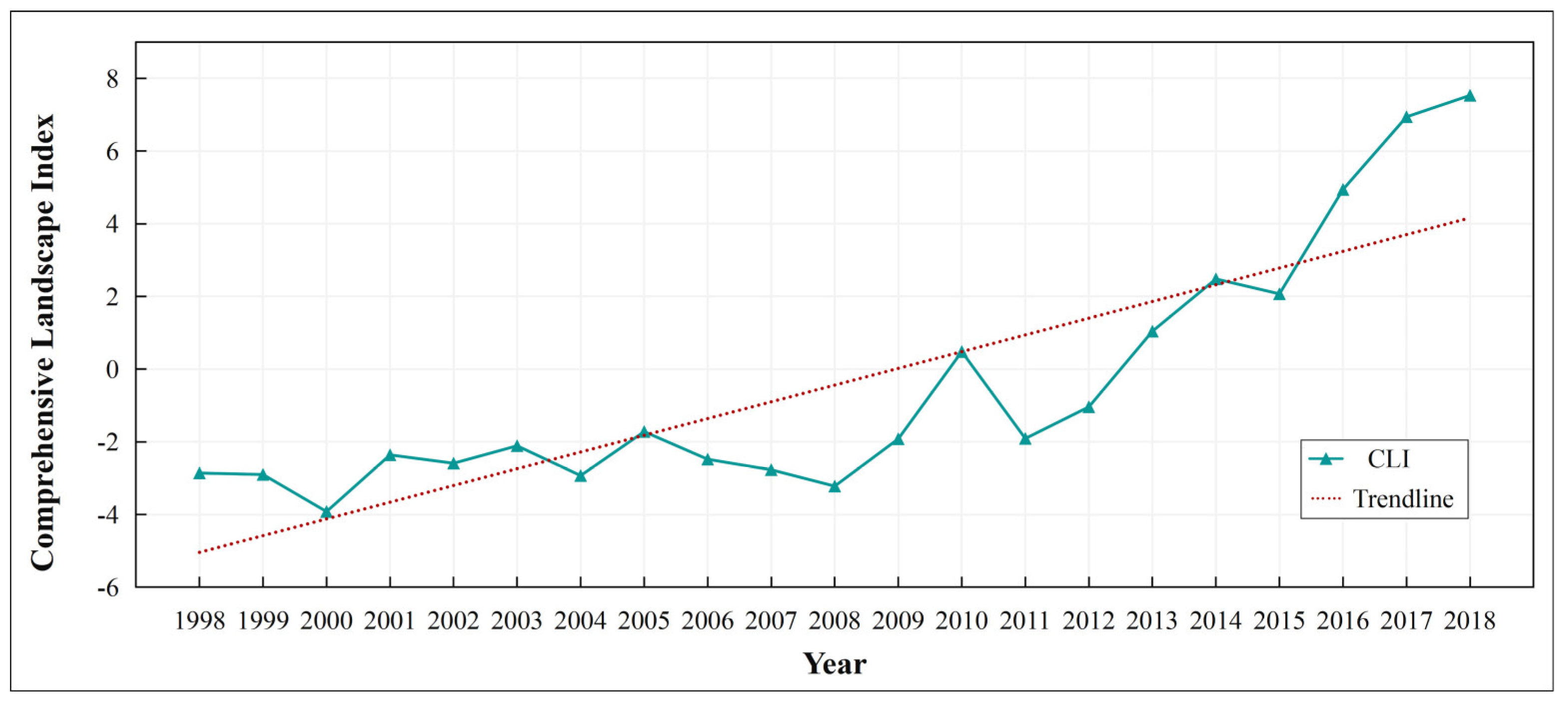
• Continuous upward trend of the CLI (1998–2018): The CLI for Minnesota showed a consistent upward trajectory over the study period. This trend indicates an increase in the density and complexity of patch shapes, signifying heightened landscape fragmentation and diversity. Concurrently, there was a deterioration in landscape connectivity and a further diversification of patch types.
• Significant mutations in 2010: The CLI experienced a notable shift in 2010, with a significant change in the dominant patch species within the landscape. This alteration is attributed to the combined effects of abrupt natural events and significant socio-economic transformations.
• Spatial clustering stability: Overall, the spatial clustering of the CLI remained stable, characterized by pronounced high-value and low-value clusters. High-value clusters (hot spots) are predominantly located in the north–central region and its surroundings, while low-value clusters (cold spots) are mainly found in the southwest and adjacent areas.
• Quantitative relationship insights: In terms of influencing factors on the CLI, POP emerged as the most sensitive, followed by AS, GDP, VS, and SLP.
• Multi-factorial influence on spatial pattern: The spatial pattern of the CLI is shaped by the interaction of multiple influencing factors rather than being dictated by a single factor. This highlights the complexity of landscape pattern formation and the need for a multifaceted approach to understanding it.
• Critical role of human activity and vegetation cover change: Among the various interactions, the synergy between human activity and changes in vegetation cover stands out as the most significant factor influencing the spatial pattern of landscape patterns.

This study underscores the intricate interplay between natural events, human interventions, and socio-economic dynamics in shaping the landscape patterns of Minnesota. The findings contribute valuable insights into landscape ecology, offering a foundation for informed decision-making in land use planning and environmental management.

References

1. Fu, F.; Deng, S.M.; Wu, D.; Liu, W.W.; Bai, Z.H. Research on the spatiotemporal evolution of land use landscape pattern in a county area based on CA-Markov model. Sustain. Cities Soc. 2022, 80, 103760. [Google Scholar] [CrossRef]
2. Hansen, A.T.; Dolph, C.L.; Foufoula-Georgiou, E.; Finlay, J.C. Contribution of wetlands to nitrate removal at the watershed scale. Nat. Geosci. 2018, 11, 127. [Google Scholar] [CrossRef]
3. Gao, J.; O’Neill, B.C. Mapping global urban land for the 21st century with data-driven simulations and Shared Socioeconomic Pathways. Nat. Commun. 2020, 11, 2302. [Google Scholar] [CrossRef] [PubMed]
4. Ren, Q.; He, C.Y.; Huang, Q.X.; Shi, P.J.; Zhang, D.; Güneralp, B. Impacts of urban expansion on natural habitats in global drylands. Nat. Sustain. 2022, 5, 869–878. [Google Scholar] [CrossRef]
5. Simkin, R.D.; Seto, K.C.; McDonald, R.I.; Jetz, W. Biodiversity impacts and conservation implications of urban land expansion projected to 2050. Proc. Natl. Acad. Sci. USA 2022, 119, e2117297119. [Google Scholar] [CrossRef] [PubMed]
6. DeFries, R.S.; Rudel, T.; Uriarte, M.; Hansen, M. Deforestation driven by urban population growth and agricultural trade in the twenty-first century. Nat. Geosci. 2010, 3, 178–181. [Google Scholar] [CrossRef]
7. Dadashpoor, H.; Azizi, P.; Moghadasi, M. Land use change, urbanization, and change in landscape pattern in a metropolitan area. Sci. Total Environ. 2019, 655, 707–719. [Google Scholar] [CrossRef]
8. Nie, W.B.; Yang, F.; Xu, B.; Bao, Z.Y.; Shi, Y.; Liu, B.T.; Wu, R.W.; Lin, W. Spatiotemporal Evolution of Landscape Patterns and Their Driving Forces Under Optimal Granularity and the Extent at the County and the Environmental Functional Regional Scales. Front. Ecol. Evol. 2022, 10, 954232. [Google Scholar] [CrossRef]
9. Zhang, Y.; Wang, T.; Cai, C.; Li, C.; Liu, Y.; Bao, Y.; Guan, W. Landscape pattern and transition under natural and anthropogenic disturbance in an arid region of northwestern China. Int. J. Appl. Earth Obs. Geoinf. 2016, 44, 1–10. [Google Scholar] [CrossRef]
10. Cui, L.; Wang, J.; Sun, L.; Lv, C.D. Construction and optimization of green space ecological networks in urban fringe areas: A case study with the urban fringe area of Tongzhou district in Beijing. J. Clean. Prod. 2020, 276, 124266. [Google Scholar] [CrossRef]
11. Liu, K.; Yang, Y.; Shi, R.; Li, Q.; Wu, B.; Zheng, H.; Mi, C. Spatiotemporal changes and driving forces of landscape patterns in the Yuqiao Reservoir watershed during 1990–2020. J. Agric. Resour. Environ. 2023, 40, 154–164. [Google Scholar]
12. Wang, H.R.; Zhang, M.D.; Wang, C.Y.; Wang, K.Y.; Wang, C.; Li, Y.; Bai, X.L.; Zhou, Y.K. Spatial and Temporal Changes of Landscape Patterns and Their Effects on Ecosystem Services in the Huaihe River Basin, China. Land 2022, 11, 513. [Google Scholar] [CrossRef]
13. Li, J.; Zhou, K.; Xie, B.; Xiao, J. Impact of landscape pattern change on water-related ecosystem services: Comprehensive analysis based on heterogeneity perspective. Ecol. Indic. 2021, 133, 108372. [Google Scholar] [CrossRef]
14. Zhang, W.; Chang, W.J.; Zhu, Z.C.; Hui, Z. Landscape ecological risk assessment of Chinese coastal cities based on land use change. Appl. Geogr. 2020, 117, 102174. [Google Scholar] [CrossRef]
15. Zambrano, L.; Handel, S.N.; Fernandez, T.; Brostella, I. Landscape spatial patterns in Mexico City and New York City: Contrasting territories for biodiversity planning. Landsc. Ecol. 2022, 37, 601–617. [Google Scholar] [CrossRef]
16. Agriculture. Available online: https://www.dli.mn.gov/business/workforce/agriculture (accessed on 29 May 2024).
17. Windmuller-Campione, M.A.; Russell, M.B.; Sagor, E.; D’Amato, A.W.; Ek, A.R.; Puettmann, K.J.; Rodman, M.G. The Decline of the Clearcut: 26 Years of Change in Silvicultural Practices and Implications in Minnesota. J. For. 2020, 118, 244–259. [Google Scholar] [CrossRef]
18. Schroeder, S.A.; Fulton, D.C. Land of 10,000 Lakes and 2.3 Million Anglers: Problems and Coping Response Among Minnesota Anglers. J. Leis. Res. 2010, 42, 291–315. [Google Scholar] [CrossRef]
19. Antrop, M.; Van Eetvelde, V. Analysing Landscape Patterns. In Landscape Perspectives: The Holistic Nature of Landscape; Landscape Series; Springer: Cham, Switzerland, 2017; Volume 23, pp. 177–208. [Google Scholar]
20. Malandra, F.; Vitali, A.; Urbinati, C.; Weisberg, P.J.; Garbarino, M. Patterns and drivers of forest landscape change in the Apennines range, Italy. Reg. Environ. Chang. 2019, 19, 1973–1985. [Google Scholar] [CrossRef]
21. Etter, A.; McAlpine, C.; Possingham, H.P. Historical patterns and drivers of landscape change in Colombia since 1500: A regionalized spatial approach. Ann. Assoc. Am. Geogr. 2008, 98, 2–23. [Google Scholar] [CrossRef]
22. Lin, J.P.; Zhu, C.H.; Deng, A.Z.; Zhang, Y.P.; Yuan, H.; Liu, Y.Y.; Li, S.R.; Chen, W. Causes of Changing Woodland Landscape Patterns in Southern China. Forests 2022, 13, 2183. [Google Scholar] [CrossRef]
23. Huang, L.; Chen, X.H.; Ye, C.X.; Yuan, Z.; He, K.L. Multiscale effects and drivers of landscape heterogeneity for water-related ecosystem services in urban agglomerations. Hydrol. Process. 2024, 38, e15081. [Google Scholar] [CrossRef]
24. Moarrab, Y.; Salehi, E.; Amiri, M.J.; Hovidi, H. Spatial-temporal assessment and modeling of ecological security based on land-use/cover changes (case study: Lavasanat watershed). Int. J. Environ. Sci. Technol. 2022, 19, 3991–4006. [Google Scholar] [CrossRef]
25. Li, B.; Jiao, S.; Zhou, M.; Zhou, Y. Effects of urban green space landscape pattern on flood retention efficiency from “urban-block” scale perspective. J. Appl. Ecol. 2024, 35, 533–542. [Google Scholar] [CrossRef]
26. Zheng, X.P.; Chen, Z. The spatial response of carbon storage to territorial space composition and landscape pattern changes: A case study of the Fujian Delta urban agglomeration, China. Environ. Sci. Pollut. Res. 2024, 31, 11666–11683. [Google Scholar] [CrossRef] [PubMed]
27. Hu, W.W.; Wang, G.X.; Deng, W. Advance in Research of the Relationship between Landscape Patterns and Ecological Pro-cesses. Prog. Geogr. 2008, 27, 18–24. [Google Scholar] [CrossRef]
28. Kim, Y.; Yu, S.Y.; Li, D.Y.; Gatson, S.N.; Brown, R.D. Linking landscape spatial heterogeneity to urban heat island and outdoor human thermal comfort in Tokyo: Application of the outdoor thermal comfort index. Sustain. Cities Soc. 2022, 87, 104262. [Google Scholar] [CrossRef]
29. Zhang, J.; Jiang, X.; Xie, X. Evolution of Traditional Village Landscape Pattern in Northwestern Yunnan’s Intermontane Basin and Its Influencing Factors: A Case Study of Dacang Village, Xiangyun County, Yunnan Province. Econ. Geogr. 2023, 43, 197–207. [Google Scholar]
30. Chen, W.X.; Zeng, J.; Chu, Y.M.; Liang, J.L. Impacts of Landscape Patterns on Ecosystem Services Value: A Multiscale Buffer Gradient Analysis Approach. Remote Sens. 2021, 13, 2551. [Google Scholar] [CrossRef]
31. Zhang, X.Y.; Li, H.W.; Xia, H.; Tian, G.H.; Yin, Y.X.; Lei, Y.K.; Kim, G. The Ecosystem Services Value Change and Its Driving Forces Responding to Spatio-Temporal Process of Landscape Pattern in the Co-Urbanized Area. Land 2021, 10, 1043. [Google Scholar] [CrossRef]
32. Yang, Y.T.; Wong, L.N.Y.; Chen, C.; Chen, T. Using multitemporal Landsat imagery to monitor and model the influences of landscape pattern on urban expansion in a metropolitan region. J. Appl. Remote Sens. 2014, 8, 083639. [Google Scholar] [CrossRef]
33. Murunga, K.W.; Nyadawa, M.; Sang, J.; Cheruiyot, C. Characterizing landscape fragmentation of Koitobos river sub-basin, Trans-Nzoia, Kenya. Heliyon 2024, 10, e29237. [Google Scholar] [CrossRef] [PubMed]
34. Hu, C.Y.; Wu, W.; Zhou, X.X.; Wang, Z.J. Spatiotemporal changes in landscape patterns in karst mountainous regions based on the optimal landscape scale: A case study of Guiyang City in Guizhou Province, China. Ecol. Indic. 2023, 150, 110211. [Google Scholar] [CrossRef]
35. Wu, C.F.; Lin, Y.P.; Chiang, L.C.; Huang, T. Assessing highway’s impacts on landscape patterns and ecosystem services: A case study in Puli Township, Taiwan. Landsc. Urban Plan. 2014, 128, 60–71. [Google Scholar] [CrossRef]
36. Zhang, Y.; Zhang, J.X.; Wang, F.Y.; Yang, W.J. Spatiotemporal Landscape Pattern Analyses Enhanced by an Integrated Index: A Study of the Changbai Mountain National Nature Reserve. Remote Sens. 2023, 15, 1760. [Google Scholar] [CrossRef]
37. Guan, C.H.; You, M.Z. Integrating landscape and urban development in a comprehensive landscape sensitivity index: A case study of the Appalachian Trail region. Urban For. Urban Green. 2024, 93, 128234. [Google Scholar] [CrossRef]
38. Yang, B.; Zheng, H.; Yin, G.; Zhao, T.; He, P.; Ouyang, Z. Research on Landscape Pattern Change in Zhangjiajie National Forest Park. Sci. Silvae Sin. 2006, 42, 11–15. [Google Scholar]
39. Xu, J.; Li, G.; Qu, J.; He, L. Changes of Land use and Landscape pattern in Hongze Lake Basin. Resour. Environ. Yangtze Basin 2011, 20, 1211–1216. [Google Scholar]
40. Chen, Y.; Tang, C.; Ma, Q.; Xue, J. Landscape pattern change of Chongming Dongtan Nature Reserve of Shanghai from 2011 to 2015. J. Nanjing For. Univ. Nat. Sci. Ed. 2017, 41, 1–8. [Google Scholar]
41. Liu, J.; Xu, Q.L.; Yi, J.H.; Huang, X. Analysis of the heterogeneity of urban expansion landscape patterns and driving factors based on a combined Multi-Order Adjacency Index and Geodetector model. Ecol. Indic. 2022, 136, 108655. [Google Scholar] [CrossRef]
42. Feng, F.; Wang, L.L.; Hou, W.X.; Yang, R.; Zhang, S.W.; Zhao, W.J. Analyzing the dynamic changes and causes of greenspace landscape patterns in Beijing plains. Ecol. Indic. 2024, 158, 111556. [Google Scholar] [CrossRef]
43. Zuo, Y.F.; Gao, J.W.; He, K.N. Interactions among ecosystem service key factors in vulnerable areas and their response to landscape patterns under the National Grain to Green Program. Land Degrad. Dev. 2024, 35, 898–915. [Google Scholar] [CrossRef]
44. Xu, L.L.; Yu, H.; Zhong, L.S. Evolution of the landscape pattern in the Xin’an River Basin and its response to tourism activities. Sci. Total Environ. 2023, 880, 163472. [Google Scholar] [CrossRef] [PubMed]
45. Shi, Y.S.; Xiao, J.Y.; Shen, Y.J.; Yamaguchi, Y. Quantifying the spatial differences of landscape change in the Hai River Basin, China, in the 1990s. Int. J. Remote Sens. 2012, 33, 4482–4501. [Google Scholar] [CrossRef]
46. Yu, D.L.; Fang, C.L. Urban Remote Sensing with Spatial Big Data: A Review and Renewed Perspective of Urban Studies in Recent Decades. Remote Sens. 2023, 15, 1307. [Google Scholar] [CrossRef]
47. Samra, R.M.A. Investigating and mapping day-night urban heat island and its driving factors using Sentinel/MODIS data and Google Earth Engine. Case study: Greater Cairo, Egypt. Urban Clim. 2023, 52, 101729. [Google Scholar] [CrossRef]
48. Nistor, C.; Vîrghileanu, M.; Cârlan, I.; Mihai, B.A.; Toma, L.; Olariu, B. Remote Sensing-Based Analysis of Urban Landscape Change in the City of Bucharest, Romania. Remote Sens. 2021, 13, 2323. [Google Scholar] [CrossRef]
49. Zhong, M.X. Impact of landscape patterns on ecosystem services in China: A case study of the central plains urban agglomeration. Front. Environ. Sci. 2024, 12, 1285679. [Google Scholar] [CrossRef]
50. Ke, L.N.; Liu, D.Q.; Tan, Q.; Wang, S.T.; Wang, Q.M.; Yang, J. Spatial-Temporal Pattern of Land Use and SDG15 Assessment in the Bohai Rim Region Based on GEE and RF Algorithms. Ieee J. Sel. Top. Appl. Earth Obs. Remote Sens. 2024, 17, 7541–7553. [Google Scholar] [CrossRef]
51. Xu, N.H.; Zeng, P.; Guo, Y.Y.; Siddique, M.A.; Li, J.X.; Ren, X.T.; Tang, F.L.; Zhang, R. The spatiotemporal evolution of rural landscape patterns in Chinese metropolises under rapid urbanization. PLoS ONE 2024, 19, e0301754. [Google Scholar] [CrossRef]
52. Chu, M.R.; Lu, J.Y.; Sun, D.Q. Influence of Urban Agglomeration Expansion on Fragmentation of Green Space: A Case Study of Beijing-Tianjin-Hebei Urban Agglomeration. Land 2022, 11, 275. [Google Scholar] [CrossRef]
53. Li, H.; Peng, J.; Liu, Y.; Hu, Y.n. Urbanization impact on landscape patterns in Beijing City, China: A spatial heterogeneity perspective. Ecol. Indic. 2017, 82, 50–60. [Google Scholar] [CrossRef]
54. Chi, Y.; Shi, H.H.; Zheng, W.; Wang, E.K. Archipelagic landscape patterns and their ecological effects in multiple scales. Ocean Coast. Manag. 2018, 152, 120–134. [Google Scholar] [CrossRef]
55. Guo, M.S.; Zhou, N.Q.; Cai, Y.; Zhao, W.A.; Lu, S.S.; Liu, K.H. Monitoring the Landscape Pattern Dynamics and Driving Forces in Dongting Lake Wetland in China Based on Landsat Images. Water 2024, 16, 1273. [Google Scholar] [CrossRef]
56. Yang, M.; Gong, J.G.; Zhao, Y.; Wang, H.; Zhao, C.P.; Yang, Q.; Yin, Y.S.; Wang, Y.; Tian, B. Landscape Pattern Evolution Processes of Wetlands and Their Driving Factors in the Xiong’an New Area of China. Int. J. Environ. Res. Public Health 2021, 18, 4403. [Google Scholar] [CrossRef] [PubMed]
57. Ma, X.; Dang, J.; Li, X.; Zhao, N. Spatial-temporal Changes and Driving Forces of Urban Landscape Pattern in Taiyuan City in Last 15 Years. Bull. Soil Water Conserv. 2018, 38, 308–316. [Google Scholar]
58. Hu, X.W.; Xu, W.W.; Li, F.Y. Spatiotemporal Evolution and Optimization of Landscape Patterns Based on the Ecological Restoration of Territorial Space. Land 2022, 11, 2114. [Google Scholar] [CrossRef]
59. Dong, L.Q.; Yang, W.; Zhang, K.; Zhen, S.; Cheng, X.P.; Wu, L.H. Study of marsh wetland landscape pattern evolution on the Zoige Plateau due to natural/human dual-effects. Peerj 2020, 8, e9904. [Google Scholar] [CrossRef] [PubMed]
60. Wang, X.M.; Meng, Q.Y.; Zhang, L.L.; Hu, D. Evaluation of urban green space in terms of thermal environmental benefits using geographical detector analysis. Int. J. Appl. Earth Obs. Geoinf. 2021, 105, 102610. [Google Scholar] [CrossRef]
61. Wu, X.P.; Zhou, Z.F.; Zhu, M.; Wang, J.L.; Liu, R.P.; Zheng, J.J.; Wan, J.X. Quantifying Spatiotemporal Characteristics and Identifying Influential Factors of Ecosystem Fragmentation in Karst Landscapes: A Comprehensive Analytical Framework. Land 2024, 13, 278. [Google Scholar] [CrossRef]
62. Li, M.Y.; Li, X.B.; Liu, S.Y.; Lyu, X.; Dang, D.L.; Dou, H.S.; Wang, K. Analysis of the Spatiotemporal Variation of Landscape Patterns and Their Driving Factors in Inner Mongolia from 2000 to 2015. Land 2022, 11, 1410. [Google Scholar] [CrossRef]
63. Liu, Q.; Wei, F.; Xia, X.; Zhang, M.; Wang, X.; Mu, X.; Xu, D. Landscape Pattern Evolution and Driving Forces of Land Use in Kuye River Basin from 1980 to 2020. Res. Soil Water Conserv. 2023, 30, 335–341. [Google Scholar]
64. Wang, S.Y.; Wang, G.Q.; Zhang, Z.X.; Zhou, Q.B. Analysis of landscape patterns and driving factors of land use in China. In Proceedings of the 23rd International Geoscience and Remote Sensing Symposium (IGARSS 2003), Toulouse, France, 21–25 July 2003; pp. 3374–3376. [Google Scholar]
65. Cheng, S.; Zeng, X.; Wang, Z.H.; Zeng, C.; Cao, L. Spatiotemporal variations of tidal flat landscape patterns and driving forces in the Yangtze River Delta, China. Front. Mar. Sci. 2023, 9, 1086775. [Google Scholar] [CrossRef]
66. Wang, J.; Xu, C. Geodetector: Principle and prospective. Acta Geogr. Sin. 2017, 72, 116–134. [Google Scholar]
67. Wang, J.F.; Li, X.H.; Christakos, G.; Liao, Y.L.; Zhang, T.; Gu, X.; Zheng, X.Y. Geographical Detectors-Based Health Risk Assessment and its Application in the Neural Tube Defects Study of the Heshun Region, China. Int. J. Geogr. Inf. Sci. 2010, 24, 107–127. [Google Scholar] [CrossRef]
68. Overview of Minnesota. Available online: http://chicago.mofcom.gov.cn/article/ddgk/a/201508/20150801072877.shtml (accessed on 29 May 2024).
69. Climate of Minnesota. Available online: https://en.wikipedia.org/wiki/Climate_of_Minnesota (accessed on 29 May 2024).
70. Urban and Rural Population. Available online: https://minnesotago.org/trends/urbanization (accessed on 29 May 2024).
71. Yuan, F. Urban growth monitoring and projection using remote sensing and geographic information systems: A case study in the Twin Cities Metropolitan Area, Minnesota. Geocarto Int. 2010, 25, 213–230. [Google Scholar] [CrossRef]
72. Wright, C.K.; Wimberly, M.C. Recent land use change in the Western Corn Belt threatens grasslands and wetlands. Proc. Natl. Acad. Sci. USA 2013, 110, 4134–4139. [Google Scholar] [CrossRef] [PubMed]
73. Forest & Ecosystems. Available online: https://climate.umn.edu/our-changing-climate/forest-ecosystems (accessed on 29 May 2024).
74. Sharma, R.; Nehren, U.; Rahman, S.A.; Meyer, M.; Rimal, B.; Seta, G.A.; Baral, H. Modeling Land Use and Land Cover Changes and Their Effects on Biodiversity in Central Kalimantan, Indonesia. Land 2018, 7, 57. [Google Scholar] [CrossRef]
75. Verburg, P.H.; Neumann, K.; Nol, L. Challenges in using land use and land cover data for global change studies. Glob. Chang. Biol. 2011, 17, 974–989. [Google Scholar] [CrossRef]
76. Mandal, D.; Singh, R.; Dhyani, S.K.; Dhyani, B.L. Landscape and land use effects on soil resources in a Himalayan watershed. Catena 2010, 81, 203–208. [Google Scholar] [CrossRef]
77. Izakovičová, Z.; Oszlányi, J. The impact of stress factors, landscape loads and human activities: Implications for sustainable development. Int. J. Environ. Waste Manag. 2013, 11, 111–128. [Google Scholar] [CrossRef]
78. Mann, H.B. Nonparametric Tests Against Trend. Econometrica 1945, 13, 245–259. [Google Scholar] [CrossRef]
79. Wang, W.; Chen, Y.; Becker, S.; Liu, B. Variance Correction Prewhitening Method for Trend Detection in Autocorrelated Data. J. Hydrol. Eng. 2015, 20, 04015033. [Google Scholar] [CrossRef]
80. Zhang, D.; Cong, Z.; Ni, G. Comparison of three Mann-Kendall methods based on the Chinas meteorological data. Adv. Water Sci. 2013, 24, 490–496. [Google Scholar]
81. Zhang, H.; Li, Z.; Xi, Q.; Yu, Y. Mann-Kendall trend test Method based on improved overbleaching. J. Hydroelectr. Power 2018, 37, 34–46. [Google Scholar]
82. Rybski, D.; Neumann, J. A Review on the Pettitt Test; Springer: Cham, Switzerland, 2011; pp. 203–213. [Google Scholar]
83. Li, S.; Lv, Z. Analysis on Abrupt Change Points of Kuye River Runoff by Mann- Kendall and Pettitt. Yellow River 2015, 37, 27–29,33. [Google Scholar] [CrossRef]
84. Bao, M.; Wallace, J.M. Cluster Analysis of Northern Hemisphere Wintertime 500-hPa Flow Regimes during 1920–2014. J. Atmos. Sci. 2015, 72, 3597–3608. [Google Scholar] [CrossRef]
85. Wentzell, P.D.; Vega Montoto, L. Comparison of principal components regression and partial least squares regression through generic simulations of complex mixtures. Chemom. Intell. Lab. Syst. 2003, 65, 257–279. [Google Scholar] [CrossRef]
86. Chang, C.W.; Laird, D.A.; Mausbach, M.J.; Hurburgh, C.R. Near-infrared reflectance spectroscopy-principal components regression analyses of soil properties. Soil Sci. Soc. Am. J. 2001, 65, 480–490. [Google Scholar] [CrossRef]
87. Geodetector. Available online: http://www.geodetector.cn/ (accessed on 29 May 2024).
88. Liu, T.; Yang, X.J. Monitoring land changes in an urban area using satellite imagery, GIS and landscape metrics. Appl. Geogr. 2015, 56, 42–54. [Google Scholar] [CrossRef]
89. Phelps, N.A. Edge Cities. In International Encyclopedia of Human Geography; Kitchin, R., Thrift, N., Eds.; Elsevier: Oxford, UK, 2009; pp. 377–380. [Google Scholar]
90. Fang, G.; Zhang, Y.; Yang, J. Evolution of Urban Landscape Pattern in Suzhou City during 1987–2009. In Proceedings of the 2nd International Conference on Civil Engineering, Architecture and Building Materials (CEABM 2012), Yantai, China, 25–27 May 2012; pp. 332–336. [Google Scholar]
91. Zhang, S.H.; Zhong, Q.L.; Cheng, D.L.; Xu, C.B.; Chang, Y.N.; Lin, Y.Y.; Li, B.Y. Landscape ecological risk projection based on the PLUS model under the localized shared socioeconomic pathways in the Fujian Delta region. Ecol. Indic. 2022, 136, 108642. [Google Scholar] [CrossRef]
92. Wang, N.X.; Yan, H.Z.; Long, K.L.; Wang, Y.T.; Li, S.X.; Lei, P. Impact of greenspaces and water bodies on hydrological processes in an urbanizing area: A case study of the Liuxi River Basin in the Pearl River Delta, China. Ecol. Indic. 2023, 156, 111083. [Google Scholar] [CrossRef]
93. Shaban, A.; Kourtit, K.; Nijkamp, P. Causality Between Urbanization and Economic Growth: Evidence from the Indian States. Front. Sustain. Cities 2022, 4, 901346. [Google Scholar] [CrossRef]
94. Nguyen, H.M.; Nguyen, L.D. The relationship between urbanization and economic growth an empirical study on ASEAN countries. Int. J. Soc. Econ. 2018, 45, 316–339. [Google Scholar] [CrossRef]
95. Zhang, Y.; Wang, H.Y.; Xie, P.; Rao, Y.X.; He, Q.S. Revisiting Spatiotemporal Changes in Global Urban Expansion during 1995 to 2015. Complexity 2020, 2020, 6139158. [Google Scholar] [CrossRef]
Figure 1. The State of Minnesota.
Remotesensing 16 02113 g001
Figure 2. Technology framework.
Remotesensing 16 02113 g002
Figure 3. PCA biplot.
Remotesensing 16 02113 g003
Figure 4. Changes in the comprehensive landscape index of Minnesota.
Remotesensing 16 02113 g004
Figure 5. CLI mutation detection in Minnesota.
Remotesensing 16 02113 g005
Figure 6. Mutation test of the single landscape index. (af) Mutation detection for landscape indices NP, PD, LPI, AI, FARFAC, and SHEI, respectively.
Remotesensing 16 02113 g006
Figure 7. Spatial clustering characteristics of the integrated landscape index.
Remotesensing 16 02113 g007
Figure 8. Socio-ecological situation in Minnesota in 2018. AS and VS for Minnesota in 2018 are shown in (a); SLP is shown in (b); GDP is shown in (c), and POP is shown in (d).
Remotesensing 16 02113 g008
Figure 9. Residual distribution of integrated landscape index fitting results. (The red markers indicate residual outliers, where the confidence interval does not straddle zero).
Remotesensing 16 02113 g009