An Ensemble Mean Method for Remote Sensing of Actual Evapotranspiration to Estimate Water Budget Response across a Restoration Landscape

Abstract

Estimates of actual evapotranspiration (ETa) are valuable for effective monitoring and management of water resources. In areas that lack ground-based monitoring networks, remote sensing allows for accurate and consistent estimates of ETa across a broad scale—though each algorithm has limitations (i.e., ground-based validation, temporal consistency, spatial resolution). We developed an ensemble mean ETa (EMET) product to incorporate advancements and reduce uncertainty among algorithms (e.g., energy-balance, optical-only), which we use to estimate vegetative water use in response to restoration practices being implemented on the ground using management interventions (i.e., fencing pastures, erosion control structures) on a private ranch in Baja California Sur, Mexico. This paper describes the development of a monthly EMET product, the assessment of changes using EMET over time and across multiple land use/land cover types, and the evaluation of differences in vegetation and water distribution between watersheds treated by restoration and their controls. We found that in the absence of a ground-based monitoring network, the EMET product is more robust than using a single ETa data product and can augment the efficacy of ETa-based studies. We then found increased ETa within the restored watershed when compared to the control sites, which we attribute to increased plant water availability.

1. Introduction

1.1. Evapotranspiration and the Water Budget

Within a closed system, the water balance equation assumes the volume of water that enters a system is equal to the amount that exits, through a series of hydrologic cycles, including precipitation, changes in the storage of water in the system, recharge into the ground, and actual evapotranspiration (ETa). For ETa, water is lost to the atmosphere through transpiration (i.e., by plants) and evaporation (i.e., from soil, rock, and water surfaces; plant interception). The quantification of water volumes in these cycles supports understanding of how humans can impact water availability and manage water resources across local, regional, and national scales. For example, effectively quantifying these cycles can inform sustainable management of agricultural water resources [1,2,3], water use and availability associated with changes in land use/land cover and restoration [4,5,6], and general water resources management for decision-making [7,8]. In the case of water storage (i.e., surface water, ground water) and surface water flows, vast ground-based networks exist to accurately measure these dynamics, including the U.S. Geological Survey (USGS) National Water Information System (NWIS) (i.e., surface water discharge, storage, groundwater) [9,10]. However, networks associated with monitoring of ETa can be spatially and temporally limited. Furthermore, ETa is notoriously difficult to measure and oft requires calculations using related variables and coefficients. ETa can vary depending on net solar radiation, surface area of water bodies, wind speed, density and type of vegetation, availability of soil moisture, root depth, reflective land-surface characteristics, and the season of year [11]. On-the-ground methods for measuring ETa are the most accurate and can be used for validation to scale other approaches to wider landscapes [12].

1.2. Quantification of Evapotranspiration

Evapotranspiration can be quantified as a portion of either the potential ET (PET) or reference ET based on various landscape and climatological factors. PET is defined as the water loss through evaporation in which there is negligible resistance to the flow of water, and represents the theoretical maximum return of water to the atmosphere [13,14]. Reference ET, on the other hand, is considered the rate of ET from a fully watered vegetative surface, and is represented theoretically by either short (i.e., grass reference—ETo) or tall (i.e., alfalfa reference—ETr) vegetation [15,16], depending on the applied methodology used to produce ETa estimates [17,18]. For this study, we assume a parallel utilization between PET and reference ET. The landscape and climatological factors are represented through a series of crop coefficients and adjustments, which are multiplied against reference ET to derive estimates of ETa [15]. Field measurements and micrometeorological variables (i.e., net radiation, wind speed, relative humidity, surface temperature) are generally used to develop the Penman–Monteith [19], Shuttleworth–Wallace [20], Priestley–Taylor [21], Turc [22,23], and multiple other models [24] to estimate ETa. However, when these variables are not available, satellite imagery affords the potential to estimate ETa fluxes.

1.3. Remote Sensing of Actual Evapotranspiration

Scientists utilize weather data and remotely sensed measurements from either optical or thermal bands to populate the various algorithms to estimate ETa. Ground-based measurements of ETa, derived from sap flux measurements as well as eddy covariance and Bowen ratio flux towers, have been used to scale plant-specific moisture flux to the landscape to achieve wide-area estimates of optical-based remotely sensed ETa [25,26]. However, it is important to understand that vegetation index ETa estimation methods were created as case studies that were developed for natural resource managers to have simple, fast, accurate and validated estimation techniques, which were most often used for decision-making related to invasive species removal, restoration, water salvage, and water availability for natural ecosystems, and furthermore, these studies produced the required ground data for validation from myriad sources to include lysimeters, sap flow sensors or flux tower networks, especially critical from uncultivated landcover [27,28]. Remote sensing ETa algorithms that were validated with these such ground-based measurements may be utilized in similar uncultivated landcover that occurs in similar climates for the purpose of creating new observations where there are a lack of ground data available [17]. New coefficients are determined for use in these un-instrumented regions and across remote sensing sensors [29,30].

Though specific methodologies vary, remote sensing utilizes spectral reflectance properties that can be used to obtain information on factors such as vegetation composition, condition, moisture flux, thermal dynamics, soil moisture, as well as net reflectance and radiation (i.e., albedo) [26,31,32,33,34,35,36]. Furthermore, remote sensing ETa products are spatially and temporally consistent, facilitating trend analysis and change detection across large landscapes [17]. In some ETa case studies, there are high coefficients of determination (r2 of 0.90) between satellite sensor resolutions [30], though an r2 of 0.75 is typically the best accuracy for remotely sensed observations of ground measurements [37,38,39].

Many remote sensing-based ETa products are readily obtainable, including those produced as associated products by the source such as the Moderate Resolution Imaging Spectroradiometer (MODIS) net Evapotranspiration/Latent Heat Flux product (i.e., MOD16A2) [40,41] and the National Aeronautics and Space Administration (NASA) ECOsystem Spaceborne Thermal Radiometer Experiment on Space Station (ECOSTRESS) products [42,43,44]. Other global- and continental-scale products are derived using datasets collected by sensors such as MODIS and Landsat’s Thematic Mapper (TM) and Operational Land Imager (OLI), including the operational simplified surface energy balance (SSEBop) algorithm [45,46,47].

However, additional processing of the imagery may be necessary to quantify and develop ETa datasets. The Google Earth Engine (GEE) cloud computing platform [48] serves as an earth-imagery repository for data sources, which can be utilized to produce various remote sensing outputs, including estimates of ETa [18,49,50]. Because of the centralized web access to these large datasets and processing resources, algorithms and results that require satellite imagery processing can be quickly developed using GEE [51].

To improve product reliability and accuracy, ensemble products combine complimentary datasets into a single product representing mean estimates. Ensemble and data assimilation products are widely and effectively used in ETa applications to remove uncertainty and extreme values [52,53,54,55], in addition to extensive use in climate, hydrologic, and applied sciences [56,57,58,59]. OpenET, for instance, develops a multi-source (i.e., ensemble) mean ETa product covering the western United States (U.S.) and has been evaluated against flux tower data to demonstrate that a remote sensing ensemble product generally outperforms individual products [54,60]. Here, a mean ETa value is calculated across multiple datasets to portray a combination of model estimates. This ensemble approach is used to explore results where ETa estimates confidently converge yet also identify a range of values from which model uncertainty or methods-based outliers can be discussed with transparency. OpenET data were not an option for use or comparison in this study because the OpenET ensemble product is not available for locations outside of the U.S.

1.4. Vegetation vs. Land Cover and a Restoration Landscape

Vegetation type and composition directly relate to the amount of water lost from the system through ETa, primarily due to factors such as root depths, plant water use, vegetation density, current growth stage, and total precipitation, thus altering the local water balance. For example, forest vegetation types, such as the subtropical dry deciduous forest, will release more water to the atmosphere than grassland or shrubland vegetation types [47,61], though there is still uncertainty related to the seasonality and location of the vegetation. In addition to temperature, excessive high heat days, precipitation, and vegetation composition will create variance in ETa [62].

Numerous studies have demonstrated increases in ETa resulting from ecohydrological restoration [63,64,65,66]. Natural infrastructure in dryland streams (NIDS) are natural forms of ecological restoration developed from rock, wood, or earthen debris used to restore hydrological and ecological function of an ecosystem, and include rock detention structures (RDS; i.e., leaky weirs, one-rock dams, gabions, check dams, trincheras), earthen berms, and beaver dams and their analogs [67]. New research quantifies increased ETa for riparian areas with beaver damming NIDS [67,68]. However, we have not identified prior research that measures the impacts of RDS on ET, and none that reflect quantitatively on its subparts (i.e., evaporation, transpiration). For instance, there is concern that NIDS-style restoration, like those resulting in beaver ponds, can increase evaporation due to increased surface water exposure [69]. Yet, related studies of sand dams (that do not leak) in Kenya show minimal loss to evaporation [70].

In the Madrean Archipelago Ecoregion of the North American Southwest, the USGS documented that riparian restoration using RDS can support maintenance and increase in vegetation, despite drought conditions and up to 5 km downstream of structures [71,72,73]. In addition, the resulting development of freshwater, sponge-like wetlands at NIDS can facilitate water-limited environments in adaptation to and mitigation of climate variability via their ability to sequester carbon, detain water, and extend the longevity and area of green growth, and associated transpiration and condensation as water vapor, thereby helping to restore and regulate increasing temperatures [67,74].

1.5. Research Objectives

The USGS is collaborating with partners to answer questions pertaining to the impacts of installing NIDS on the water budget at a dryland ranch in Baja California Sur, Mexico [75,76]. In this study area, hydrogeological instrumentation, recording observations, modeling hydrogeological scenarios, and an interdisciplinary scientific study of the watershed interactions between water, ecological systems, and human activities are being conducted.

This paper describes research to estimate baseline evapotranspiration rates in a degraded tropical broadleaf deciduous forest and predict how watershed restoration using NIDS is impacting potential transpiration and plant water use, vegetation response to ecohydrological restoration using NIDS, given feedback between ecological processes and the hydrological cycle, and effects of land use/land cover change. However, there is not a ground-based ETa monitoring network (e.g., flux towers) within this study site, requiring a fully remote sensing-based approach.

We compare an ensemble mean technique with various remote sensing ETa algorithms, to address the overarching questions about how the water budget varies and how water may be allocated differently to ETa when NIDS restoration is being implemented, while also considering the partitioning of E and T. More specifically, we develop a methodology to perform the following steps: (i) produce a consistent ensemble mean ETa (EMET) product in a dryland environment using a series of independent remote sensing ETa datasets, (ii) evaluate ETa dynamics across different land-use/land-cover (LULC) types, and (iii) quantify the impacts of restoration on ETa across a restoration landscape case study. This research provides improved estimates of water use to enhance the understanding of local groundwater supplies.

2. Materials and Methods

2.1. Los Planes Basin

The Los Planes basin is in the southern portion of the state of Baja California Sur (BCS), Mexico (MX), southeast of La Paz, MX, and extends south from El Jalito to the upland elevations south of the town of La Venta (Figure 1). The basin has an area of 912 km² and extends roughly 25 km east-to-west and 50 km north-to-south.

The basin is generally structured as a sink-based dendric network, where high elevation mountain ranges largely enclose and flow directly into the central basin, which opens on only a single side. For the Los Planes basin, the central basin opens at sea level on the northeastern end at Bahía de la Ventana, while rising in elevation as high as ~1400 m across the surrounding mountain ranges to the east, south, and west. Despite these heights on the southern and eastern sides, elevations generally only reach a maximum height between 600 and 800 m on the western side.

Most of the population within the basin resides in the lower basin and along the coastal boundary, though population centers, including San Antonio, La Ventana, and Los Planes, can be found throughout upland portions of the basin (Figure 1).

Vegetation within the Los Planes basin, identified using the North American Land Change Monitoring System (NALCMS) 2015 North American Land Cover 30 m dataset [77], primarily consists of a mix of shrubland and areas of grassland across the lower elevation central valley with tropical broadleaf deciduous forest across much of the uplands on the periphery of the basin (Figure 1). An area of temperate broadleaf forest is present at the highest elevations on the southern portion of the basin. Additionally, year-round agriculture (referred to as cropland in the NALCMS dataset and hereafter), that is fed by rain and groundwater, is present at the northern portion of the central valley, surrounding San Juan de los Planes. Barren land can be found along many of the later floodplains extending from the uplands into the central valley.

The Los Planes basin is located within a semi-arid, dry tropical climate and features a unimodal precipitation regime, in which a majority of precipitation occurs during the summer and fall seasons [78]. The winter and spring seasons are typically dry. In an adjacent basin (i.e., La Paz basin to the west), average yearly precipitation is 265 mm/year [79]. However, total precipitation in the region is dependent on the presence of El Nino–Southern Oscillation (ENSO) events [80] in addition to tropical cyclones that originate at the equator and move north along the western coast of Mexico, typically from August through October [81]. These storms can bring substantial precipitation amounts to the region [81]. Examples include Hurricane Henriette, where 229.1 mm of precipitation was measured at the town of Los Planes, BCS in September 2007 [82], and Hurricane Jimena, which rained as much as 487 mm in 2009 [83]. Higher precipitation totals generally occur across the higher elevations.

Restoration Landscape—Paired Watersheds at the Research Ranch

The research ranch is a 250-acre working ranch in the Sierra Cacachilas mountains along the far western edge of the Los Planes basin. This ranch consists of three separate properties (Figure 1). The easternmost property was acquired in 2010, while the central and westernmost properties were acquired in 2021 and later. The ranch serves as a research base of operations and has applied several restoration applications since its acquisition, including the use of NIDS [67] and fencing to limit free livestock grazing.

In cooperation with the research ranch, the USGS delineated five potential study watersheds (Figure 1) using a high-resolution digital elevation model (DEM) [75]. Using a statistical analysis of each watershed’s respective structural, biophysical, and modeled hydrologic traits [84], paired watersheds of similar traits were identified that would allow for the evaluation of impacts of land management on the water budget. In a paired watershed approach, one watershed serves as a “treated” (i.e., restoration) watershed, while the statistically paired watershed remains unchanged and serves as a “control”. This pairing allows for the opportunity to monitor the changes associated with restoration.

Watershed 1 serves as the “restoration” watershed by study design. It contains a ranch property that was acquired in 2010 and has experienced numerous restoration applications including the use of fencing to stop grazing (i.e., goats, cows) and the construction of NIDS. Fencing was placed around the property boundary in 2010, while NIDS construction began in 2010 and continued in 2017 and 2019. Watershed 4, which is located within the 2021 acquisition and has remained unmanaged throughout our study period, was identified as the statistically paired watershed, and thus is considered as the formal “control” watershed in this study. Additional NIDS structures, visible in high-resolution imagery, had been placed in watershed 2 and 3, though no fencing was present during the study period. This disqualifies watersheds 2 and 3 as formal control watersheds. Watershed 5, like watershed 4, was unmanaged across the study period, but was not statistically paired to watershed 1. Though we include results for watersheds 2, 3, and 5, to allow for comparison of general conditions, they do not represent statistical pairs and, therefore, may have a dissimilar ecological response to restoration.

2.2. Remote Sensing Analyses

Using remotely sensed data as input, ETa estimates are primarily quantified using either an energy balance (i.e., heat flux)-based approach, or for those that apply using meteorological data and vegetation index products, by using the Penman–Monteith equation [35]. For both approaches, ETo is quantified through climatological factors. The energy balance approach assumes that latent heat flux, representing the difference between net radiation and outgoing flux, can be converted into an estimate of ETa [18,46,85]. Energy balance-based models primarily utilize land surface temperature (LST) for approximations of net radiation fluxes, which partially replace crop coefficients in the calculation of ETa based on evaporative cooling [35,86]. Contrarily, the meteorological-based approaches generally rely on quantifying the atmospheric water demand to estimate ETa [17,35]. These approaches then apply vegetation index measurements to represent landscape factors [17,40].

We develop and acquire a series of remote sensing-based ETa products (Figure 2) that are derived using both the energy balance- and meteorological-based approaches. Each product included in this study consists of a range of available dates, spatial, and temporal resolutions.

2.2.1. Nagler-ET(EVI2)

The Nagler vegetation index-based ETa algorithm, hereafter referred to as Nagler-ET(EVI2), was developed to estimate riparian plant consumptive use across arid and semi-arid landscapes [17]. Similar vegetation and climate traits are present across the Los Planes basin. This approach applies a remote sensing-based vegetation index (i.e., EVI2, see below) and climate variables (i.e., daily percentage of annual daytime hours, mean daily temperature) in the calculation of potential ET (see below), which are then used in a crop coefficient-based ETa algorithm [17,25]. Applying the methodology described in [17], we developed this ETa product in the GEE cloud computing interface [48] for the Los Planes basin.

We use the Enhanced Vegetation Index—2 (EVI2) to quantify vegetation greenness [87] (Equation (1)). EVI2 applies a combination of the near infrared (NIR) band, the red band, and a series of coefficients in its algorithm, which we use to compute across the full suite of images using the following equation:

EVI2 = 2.5 ∗ ((NIR − Red)/(NIR + (2.4 ∗ Red) + 1)),

(1)

A near-continuous series of Landsat images is available from January 1982 to present day (i.e., July 2023 at the time of production) when including the full suite of Landsat sensors, that is the Landsat 4 Thematic Mapper (TM) to the Landsat 9 Operational Land Imager 2 (OLI-2) [88,89]. Specifically, Landsat imagery is available on a 16-day repetition cycle for each sensor, though overlapping sensors can result in increased data collection during those times of overlap. For instance, increased coverage of satellite measurements occurs following 31 October 2021, while both Landsat 8 and Landsat 9 collect imagery simultaneously. For Landsat 7, though it continued to collect data through August 2016, data quality across our study area was impacted by the failure of the scan line corrector (SLC) on 31 May 2003 [90], resulting in the loss of roughly 15.3% of each image; therefore, to reduce additional complications by filling data gaps, we do not include Landsat 7 imagery in this analysis. Finally, to match the temporal availability of other data products, we limit our study period to January 2006 through to December 2021 (see Daymet and MODIS below).

The Nagler-ET(EVI2) model applies interpolated climate data to calculate the reference ET (ETo-c; climate based) (Equation (2)), using the Blaney–Criddle algorithm [91,92], which follows:

ETo-c = P ∗ (0.457 ∗ Tmean + 8.128),

(2)

Tmean = (tmin + tmax)/2,

(3)

P = (dayl/15,768,000) ∗ 100,

(4)

where P is the mean daily percentage of annual daytime hours and Tmean is the mean daily temperature calculated as the average of the daily maximum and daily minimum temperatures [17]. We use the Daymet V4: Daily Surface Weather and Climatological Summaries [93] product in GEE, which provide 1 km gridded estimates of weather parameters, including duration of daylight (band dayl) and minimum and maximum daily temperatures (bands tmax and tmin, respectively) on a daily time scale for North America. Tmean is calculated as the average of the sum of the minimum (i.e., tmin) and maximum (i.e., tmax) temperature for the day (Equation (3)), while P is calculated as the daily duration of daylight (i.e., dayl) divided by the annual daytime hours (50% of annual hours, in seconds), multiplied by 100 (Equation (4)), representing the daily percentage of annual daytime hours. We produce an ETo-c value for each day, then produce a mean value for the 16 days prior to the Landsat collection.

Finally, ETa is calculated using the following equation (Equation (5)) [17]:

ETa = ETo-c ∗ (1.65 ∗ (1 − (e^(−2.25 ∗ EVI2)) + 0.169)),

(5)

where ETa is actual ET and e is equal to approximately 2.718.

Nagler-ET(EVI2) is developed at a spatial resolution of 30 m due to the use of Landsat imagery in calculating the EVI2 layer. Using the ETa products for each single Landsat image, we produced a monthly mean raster across all images from each respective month. We completed this for all months in the timeseries, representing mm/day for each day within the respective month.

2.2.2. SSEBop-LS

The second Landsat-based product used in this study is the Operational Simplified Surface Energy Balance (SSEBop) model for Landsat imagery [47], hereafter referred to as SSEBop-LS. The SSEBop-LS applies a thermal-based energy balance approach using a series of Landsat-based inputs, including LST and a derived vegetation index (i.e., normalized difference vegetation index—NDVI). Additional inputs include air temperature, a digital elevation model, net radiation, and reference ET [47].

Scenes of SSEBop-LS estimated total ETa are available globally across the full suite of Landsat sensors (i.e., 1982 to present-day) [89], accessible through the USGS Earth Resources Observation and Science (EROS) Center Science Processing Architecture on Demand Interface [94] (https://espa.cr.usgs.gov/; accessed on 22 June 2023). To download imagery, the user must provide a list of Landsat Collection-2/Level-2 scene identification numbers. We recalled the list of Landsat scenes that were used to develop the Nagler-ET(EVI2) product and ingested this list as requested ETa products from the EROS Science Processing Architecture (ESPA) [94]. We projected and clipped all images (n = 367) to the study area, in addition to masking based on the respective pixel quality assessment band provided by the ESPA.

To align temporally with the Nagler-ET(EVI2) product, we converted the single Landsat images into monthly mean raster products using the same approach applied to develop monthly means for the Nagler-ET(EVI2) product. Lastly, this product required a scaling factor of 0.001 to convert to mm/day for each month.

2.2.3. SSEBop-MOD

The SSEBop algorithm was developed using imagery collected by MODIS to provide an ETa product which could be used to inform an early-warning system for drought monitoring [45,46]. Imagery products from MODIS are collected daily at a spatial resolution ranging from 250 m to 1 km, depending on the band [95]. The SSEBop MODIS-based model, hereafter referred to as SSEBop-MOD, applies MODIS-derived products, specifically LST, emissivity, NDVI, and albedo [46] to calculate latent heat flux, similar to the approach applied for SSEBop-LS.

The SSEBop-MOD product is available at a global scale at a spatial resolution of 1 km from January 2003 through to April 2022, and can be downloaded on a monthly timescale through the U.S. Geological Famine Early Warning Systems Network (FEWS NET) data portal [96] (https://earlywarning.usgs.gov/fews; accessed on 8 June 2023). We downloaded all monthly ETa images from January 2006 to December 2021. We then projected and clipped the images to the Los Planes basin. Following conversion to a daily estimate, by dividing by the respective number of days per month, the unit for this product is mm/day per month.

2.2.4. MODIS—MOD16A2

We include the MODIS-MOD16A2 product in this study, hereafter MODIS-ET, which—similar to Nagler-ET(EVI2)—is a vegetation index-based product [40]. This product provides an 8-day composition of ETa estimates with a spatial resolution of 500 m. The MODIS-ET product applies a variation of the Penman–Monteith equation by considering factors of leaf area index, soil heat fluxes, and fractional solar radiation [40]. The Version 6 product is available, as an 8-day composite of ETa within the GEE repository, beginning in 2001 [41].

Using the 8-day ETa composite band, we averaged all images across each month from January 2006 to December 2021 (n = 192) for the Los Planes basin, masking for clouds and overall pixel quality using the pixel quality control band (i.e., ET_QC). We then scaled the product (i.e., by 0.1) and divided the monthly 8-day mean by 8 to calculate mean daily ETa, which we used to quantify total monthly ETa. After the application of scaling and conversion factors the product is presented in mm/day.

2.3. Evapotranspiration Data Harmonization

There was variability in the spatial resolution, temporal resolution, and temporal coverage of each of the base ETa products (

Table 1. Listing the source’s respective spatial resolution, temporal resolution, and temporal coverage for each of the evapotranspiration products, and for the data harmonization product. The range for Source temporal coverage is listed for at the time of development in September 2023, while “Present day *” refers to availability of the dataset at the point of development in September 2023.

ETa Algorithm	Source Spatial Resolution	Source Temporal Resolution	Source Temporal Coverage
Nagler-ET(EVI2)	30 m	16 day	August 1982–December 2021
SSEBop-LS	30 m	16 day	August 1982–Present Day *
SSEBop-MOD	1000 m	1 month	January 2003–April 2022
MODIS-ET	500 m	8 day	January 2003–Present Day *
Data Harmonization	30 m	1 month	January 2006–December 2021

). To allow for both a direct comparison between the various ETa products and to coalesce into a single ensemble-based product, it was imperative that the various ETa products aligned spatially and temporally. To align temporally, we constrained each product to a range of 2006 through to 2021, which aligns with availability of the products. For instance, the MODIS-based products are available beginning in January 2001 while Daymet climate data, used to calculate the Nagler-ET(EVI2) product, are not available (at the time of production) after December 2021. Furthermore, there was limited Landsat data availability across the Los Planes basin between 2003 and 2006. Therefore, we identified a 192-month period (i.e., January 2006 through to December 2021; 16 years) in which ETa products can be directly compared. Due to the presence of occasional quality control factors (i.e., cloud cover, aerosols, pixel quality, radiometric saturation) established for both the MODIS and Landsat imagery [97,98], not all months provide coverage of ETa across the full watershed. For instance, the Nagler-ET(EVI2) vegetation product is not available for 29 months (i.e., ~15.1%), with multi-month periods of missing data, particularly from November 2011 to April 2013 (18 months). The SSEBop-LS product, by including the same base Landsat imagery, has duplicate limitations. Similarly, the MODIS-ET product was corrected to account for quality control, and cloud cover and other obstructions were masked. To visualize this, we developed maps that show the percent of months (i.e., of 192 months) in which an ETa value is present for each product.

Then, as discussed throughout the previous section, we converted all products (if necessary) into monthly means to allow for a more direct and long-term comparison. Specifically, the SSEBop-MOD product is downloaded as monthly means while the Nagler-ET(EVI2), SSEBop-LS, and MODIS-ET products all require aggregation to monthly means due to there being multiple images per month. Therefore, monthly values represent daily mean estimates for the respective month, and we converted all ETa values to mm/day to allow for direct comparison between products.

Spatial harmonization was applied by resampling each input product to 30 m using the nearest neighbor technique in ArcMap to produce the ensemble product at the highest resolution possible. A nearest neighbor approach was applied to spatially align the lower-resolution base products (i.e., SSEBop-MOD = 1 km/MODIS-ET = 500 m) with the higher-resolution base products (i.e., SSEBop-LS/Nagler-ET(EVI2) = 30 m), while retaining the original pixel values thus allowing variability in the EMET product to result from variability within the higher-resolution products.

2.4. Ensemble Mean

We define an ensemble as an aggregation of similar and complimentary components that can contribute to a single effect. We developed the watershed-scale monthly EMET product by averaging the MODIS-ET, SSEBop-MOD, SSEBop-LS, and Nagler-ET(EVI2) products for each month. Because the ensemble mean was applied to reduce data uncertainty and improve reliability by averaging multiple inputs (i.e., where and when available), in addition to improving spatial continuity for areas of missing data from a single-input ETa product, estimates were developed in some locations using less information. For instance, in months where the Landsat-based imagery for ETa products (i.e., Nagler-ET(EVI2), SSEBop-LS) is not available (Figure 2), following the suspension of image transmission (i.e., 2011/2012) [99] or if clouds fully obscured the watershed at the time of the image, we chose to not produce mean values for the EMET product (i.e., “nodata” months; n = 29 of 192). However, in months in which partial imagery is available for the Landsat-based ETa inputs, a mean value is produced by averaging inputs from any overlapping products. This may allow for potential data gaps in portions of the EMET product, though a mean value is still produced. The full timeseries of imagery is published [100].

2.5. Analysis—Comparison of Evapotranspiration Products

We completed a series of analyses to compare the EMET to the full suite of products to assess how the products compare both temporally and spatially. First, a monthly timeseries for the full watershed for each product was calculated. This timeseries shows a direct comparison between the various products, averaged across the watershed, across all months. We also compared a timeseries of the EMET product for the Los Planes basin with EMET averaged across the research ranch. For each timeseries, a series of statistics was derived, including Pearson correlations, root mean square error (RMSE), and mean absolute error (MAE), to measure their comparability. Relatively strong correlations and low RMSE and MAE were anticipated due to similarities in the seasonality (i.e., wet and dry seasons) of the products.

Second, we completed a spatially explicit Pearson correlation between each of the respective ETa products, which develops a correlation value for each pixel across the series of months, using R software version 4.2.2 and ArcGIS 10.8 [101,102]. This analysis shows how the products compare spatially across the watershed and highlights areas of the watershed where correlations may be lower.

Using the EMET product, monthly mean images across the study period were produced. For example, the mean January value for all pixels was calculated from 2006 to 2021, which equates to a total of 16 years, or 16 input images for each month.

2.6. Change Analysis

2.6.1. Land Use/Land Cover and Evapotranspiration Rates

We quantified the relationship between ETa and LULC within the basin by evaluating the temporal variability of ETa in response to LULC as well as calculating and comparing spatiotemporal trends of ETa and vegetation metrics. First, we developed two timeseries of ETa for each of the LULC classes. The first timeseries shows the mean monthly value for each NALCMS LULC class for January 2006 through December 2021. This shows the range and variability between the LULC classes and portrays long-term trends. Second, we calculated monthly means across the full timeseries to show the monthly variability between LULC classes using box plots, where each month represents values across the 16-year study period. Combined, the timeseries demonstrates the seasonal and long-term patterns that are present between LULC and ETa.

Next, we used the linear Sen’s slope trend [103] to assess spatially explicit patterns in both ETa and vegetation metrics. We used the EMET product to monitor the linear trend in ETa. As a proxy to represent changes in LULC, which represents only a single point in time, we use a vegetation greenness index. Specifically, to monitor vegetation conditions, we produced a monthly NDVI product using Landsat imagery for the Los Planes basin for all months across the study period. The NDVI is a metric of vegetation greenness and overall plant photosynthetic activity [104], and is typically representative of vegetation activity [105]. NDVI values closer to 0 generally align with rock and barren soil, while values closer to 1 generally represent dense vegetation cover. We then completed a linear Sen’s slope trend analysis using the NDVI images to assess trends in vegetation greenness. Because the ETa algorithms consider vegetation greenness in the quantification of ETa, we anticipate inherent similarities in the directionality and rate of trends.

2.6.2. Watershed Restoration at the Research Ranch

To directly measure the response to restoration on the landscape, a case study across a series of watersheds within the research ranch was examined. We aim to identify how the culmination of separate restoration strategies, including (i) fencing to reduce impact from goats and cattle, (ii) impoundment structures along the arroyo bed, and (iii) erosion control structures (i.e., NIDS) within the channels and lateral slopes may impact the water budget response, by comparing changing conditions across a restoration watershed, its paired control, and a series of additional adjacent watersheds.

2.6.3. Partitioning Evaporation and Transpiration

Though ETa represents total water loss through a combination of evaporation (E) and transpiration (T), the partitioning of E and T can inform water-resource management about water that may be lost to evaporation versus water that is being transpired by plants. Both E and T have been associated with relative measurements of vegetation cover, where greater vegetation cover results in increased transpiration and reduced vegetation cover results in increased evaporation [106,107]. Furthermore, [108] documented a linear relationship between EVI and T, while [109] quantified a strong linear relationship between NDVI and E in water-restricted environments. To partition E and T for the Los Planes basin, we applied a linear parameterization between vegetated and unvegetated pixels using a remote sensing vegetation index. Specifically, we developed monthly NDVI images for all months from January 2006 to December 2021 to portray the percentage of vegetation cover. To identify appropriate thresholds for the Los Planes basin, we placed a series of points (i.e., 50 points each) along barren areas (i.e., flow channels, non-vegetated land) and areas of dense vegetation (i.e., dense upland forest), and extracted NDVI values across the full timeseries. Based on this analysis, we identified representative watershed thresholds of 0.1 for 0% cover (i.e., barren land) and 0.9 for 100% cover (i.e., dense vegetation), representing 1 standard deviation below and above the mean value for the points, respectively. Using those thresholds, we derived the percentage of vegetation cover for each NDVI monthly image. We then parsed E and T, both in mm/day, across the Los Planes basin on a monthly scale using the following equations:

T = ETa ∗ Percent Cover,

(6)

E = ETa ∗ (1 − Percent Cover),

(7)

where, ETa represents the EMET and Percent Cover represents the percentage of vegetation cover in the image.

These partitions were used to assess impacts of restoration across the research ranch. Specifically, we develop a timeseries of EMET, NDVI, E, and T for each of the watersheds across the study period. We then calculate the linear Sen’s slope of the timeseries both prior to the restoration (i.e., 2006 through 2009) and following the restoration (i.e., 2010 through 2021) to identify potential differences associated with restoration applications.

2.7. Identifying Evapotranspiration Associations with Precipitation

Though a direct linear relationship between precipitation and ETa was not anticipated [110], precipitation can be a determining factor, or predictor, in changes in ETa. To measure precipitation across the watershed, we used the Daymet V4: Daily Surface Weather and Climatological Summaries product [93] to produce monthly summations of precipitation across the watershed. The Daymet daily total precipitation spatial layer provides daily summaries of precipitation at a spatial resolution of 1 km. We developed monthly precipitation rasters from January 2006 to December 2021 by summing the daily images across each month for the Los Planes basin. We used this layer to monitor the effects of precipitation on measurements of ETa throughout this study.

3. Results

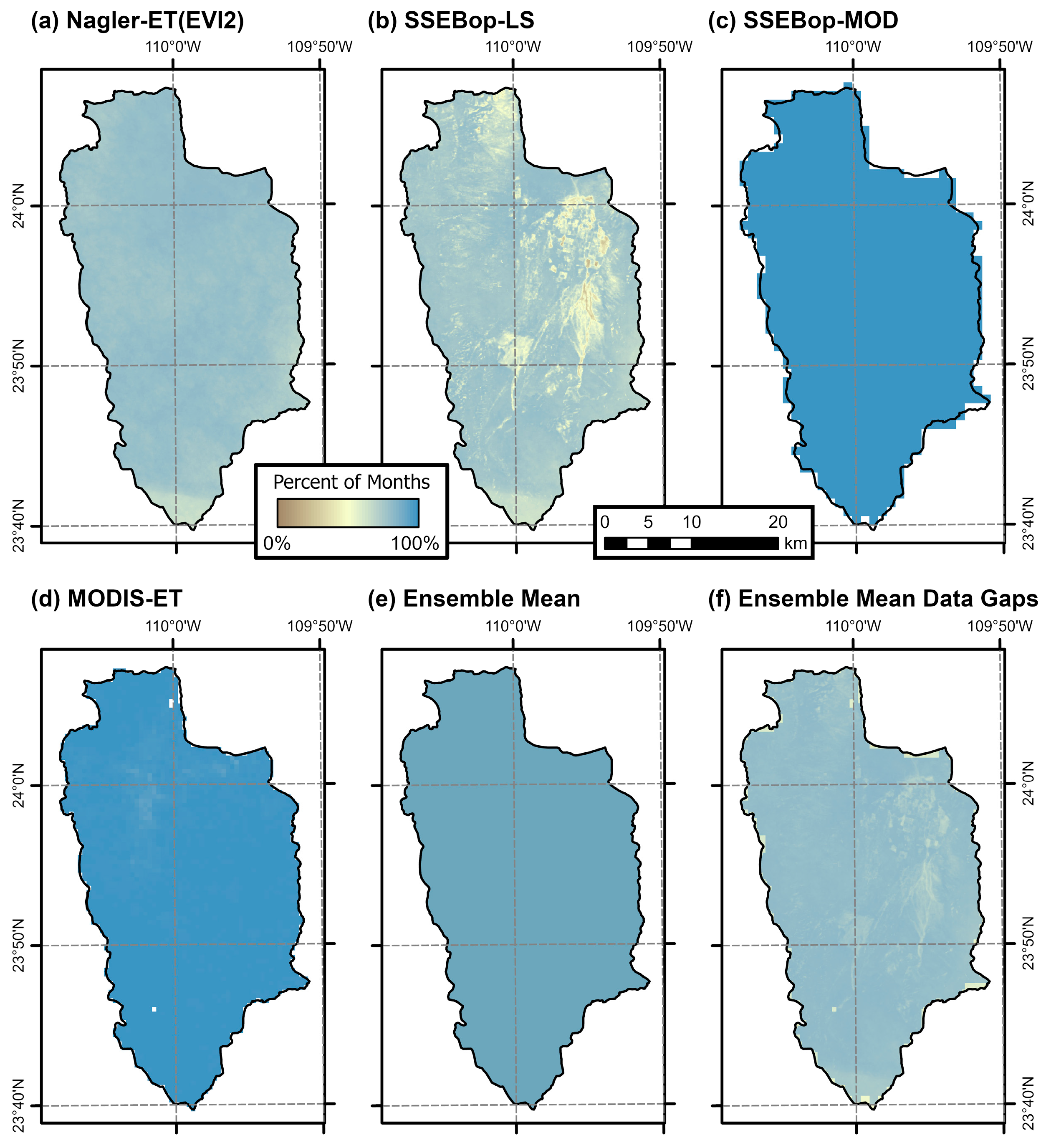
3.1. Remote Sensing Data Coverage

The percent coverage of clear pixels (i.e., following the quality control review), depicting the number of months where remotely sensed data were available by location, varied for each of the input ETa products across the watershed (Figure 3). The MODIS-based products, which collect daily imagery, have the greatest percentage of available months with a minimum cover of 93.2%, or 179 months, observed in the MODIS-ET (Figure 3d) product. The SSEBop-MOD (Figure 3c) product has full coverage across the watershed for all months. Contrarily, because several months (i.e., 29 of 192) are not available due to collection issues (i.e., 16-day repetition cycle) and quality checks (i.e., cloud cover), the two Landsat-based products have less consistent coverage over the study period. For instance, the highest percentage of coverage is for the Nagler-ET(EVI2) (Figure 3a) product, with 83.3%. The SSEBop-LS (Figure 3b) product, though having a similar maximum percentage value (i.e., 82.3%), applies a different quality control review (e.g., including radiometric saturation), and therefore, has comparatively lower clear pixel count. Furthermore, generally lower coverage is apparent throughout the east-central portion of the watershed for SSEBop-LS. Finally, the EMET (Figure 3e) product has full spatial coverage of the basin for 163 of the 192 months (i.e., 84.9%), while the remaining 29 months were not included (see 2.4 ensemble mean). However, some data gaps are present in the EMET product (Figure 3f) because of occasional “nodata” pixels within each of the single-input ETa products. The data gaps are generally more prevalent in areas aligning with reduced coverage in the SSEBop-LS product.

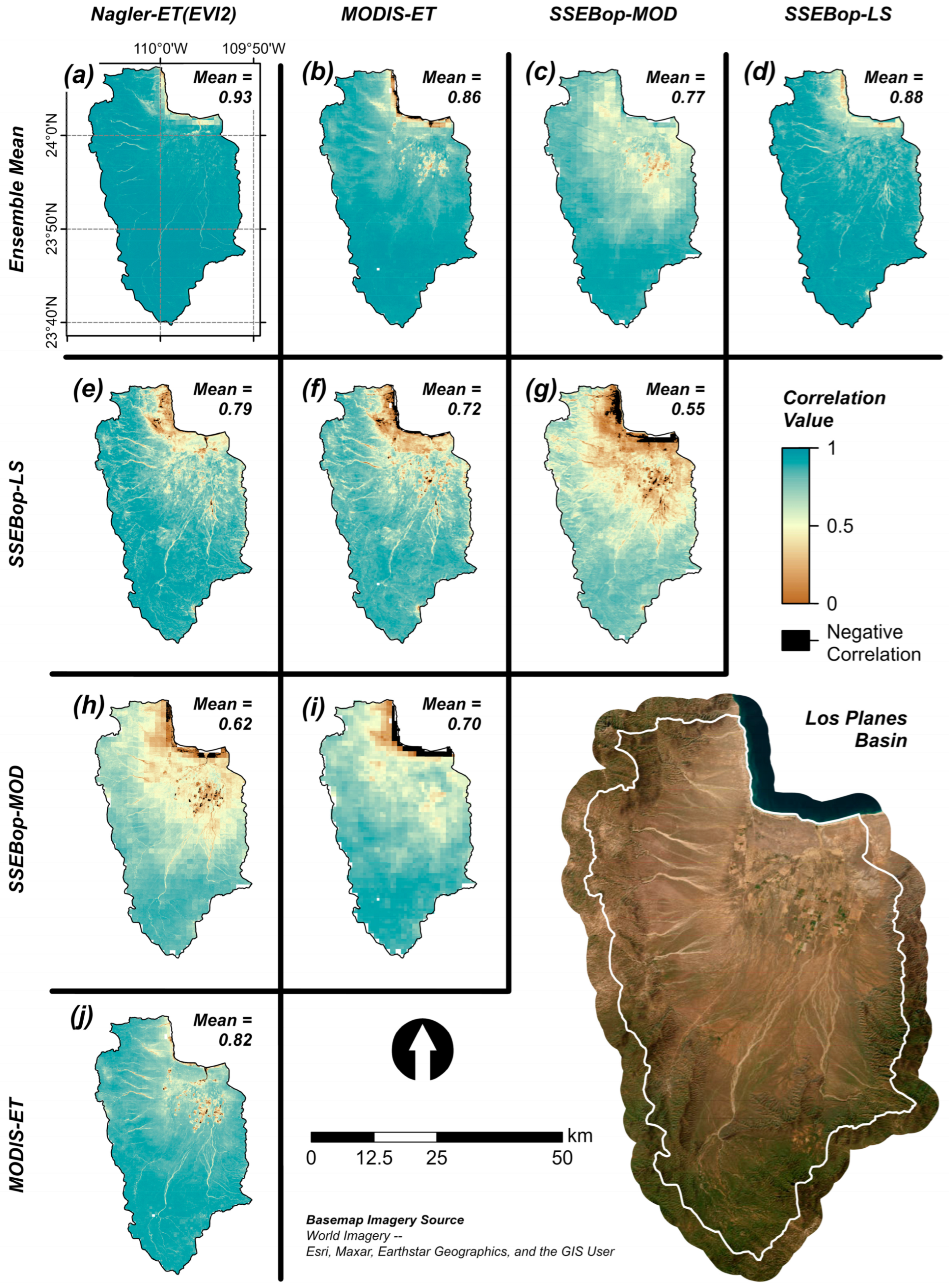
3.2. Comparison of Remote Sensing Evapotranspiration Products

The timeseries shows a range of values across the full suite of ETa products for the Los Planes basin (Figure 4a). In general, values across the timeseries show a decline in ETa for all products between 2006 and 2011 followed by a period between 2014 and 2021 in which ETa remains relatively stable, with overall lower values occurring in 2020.

Overall, the Nagler-ET(EVI2) model produces the highest values for all months where data are available, on average by roughly 3.5× (i.e., 3.1× MODIS-ET; 7.8× SSEBop-MOD; 1.3× SSEBop-LS; 1.8× EMET). It is also strongly and significantly correlated to the other products (

Table 2. Confusion matrix showing the monthly correlation (Cor), root mean square error (RMSE), and mean absolute error (MAE) between each of the evapotranspiration products averaged across the Los Planes basin. All correlations are significant (p-value < 0.001).

	Ensemble Mean (EMET; ETa)	Nagler-ET(EVI2)	SSEBop-LS	SSEBop-MOD	MODIS-ET
Ensemble Mean (EMET; ETa)	Cor = 1 RMSE = 0 MAE = 0
Nagler-ET(EVI2)	Cor = 0.97 RMSE = 0.92 MAE = 0.84	Cor = 1 RMSE = 0 MAE = 0
SSEBop-LS	Cor = 0.95 RMSE = 0.43 MAE = 0.38	Cor = 0.97 RMSE = 0.61 MAE = 0.49	Cor = 1 RMSE = 0 MAE = 0
SSEBop-MOD	Cor = 0.88 RMSE = 0.75 MAE = 0.67	Cor = 0.8 RMSE = 1.64 MAE = 1.51	Cor = 0.76 RMSE = 1.13 MAE = 1.04	Cor = 1 RMSE = 0 MAE = 0
MODIS-ET	Cor = 0.95 RMSE = 0.44 MAE = 0.4	Cor = 0.9 RMSE = 1.34 MAE = 1.23	Cor = 0.9 RMSE = 0.82 MAE = 0.76	Cor = 0.87 RMSE = 0.42 MAE = 0.34	Cor = 1 RMSE = 0 MAE = 0

) (i.e., 0.97 with SSEBop-LS; 0.97 with EMET; 0.9 with MODIS-ET; 0.8 with SSEBop-MOD). Due to similar source data, a high correlation was anticipated between the Nagler-ET(EVI2) and SSEBop-LS products despite the use of different reference ET sources used in the development of the products (i.e., ETr for SSEBop-LS and ETo-c for Nagler-ET(EVI2)). Similarly, the MODIS-based products had the highest correlations between themselves (MODIS-ET and SSEBop-MOD correlation value = 0.87), though again considering the use of different reference ET data sources. The SSEBop-MOD product has the lowest mean monthly values for all months except June and July, where the MODIS-ET is lower each year. In general, the MODIS-based products had lower values compared to the Landsat-based products.

Overall, the EMET product was strongly and significantly correlated with the full suite of products (i.e., 0.97 with Nagler-ET(EVI2); 0.95 with SSEBop-LS; 0.95 with MODIS-ET; 0.87 with SSEBop-MOD), implying a high level of association with all input products. However, both root mean square error (RMSE) and mean absolute error (MAE) were not always lower between the EMET and input products (Table 2). For instance, RMSE and MAE were lower between the MODIS-based products directly than between the MODIS-based products and the EMET product, despite higher correlations in the latter. Similarly, despite a stronger correlation between the Landsat products, both RMSE and MAE were lower between the SSEBop-LS and EMET products than the Landsat products directly. The Nagler-ET(EVI2) and EMET products had higher RMSE and MAE values compared to the two Landsat products directly.

The research ranch has slightly lower EMET values (i.e., 0.9×) compared to the full Los Planes basin (Figure 4b), particularly in 2011, 2014, and 2015. However, with a greater coefficient of variation (research ranch = 0.67; Los Planes basin = 0.64), the research ranch has, respectively, higher values in the summer (i.e., June–August; 0.97×) than in the winter (i.e., December–February; 0.85×) compared to the EMET for the Los Planes basin. Nonetheless, the two regionally scaled timeseries are strongly correlated (0.95, p-value < 0.001).

The spatiotemporal Pearson correlation maps show the relationship between each of the ETa models across the basin (Figure 5). Generally, across all four input ETa products (Figure 5e–j), the lowest correlation occurs in the northern portion of the watershed, particularly along the coast of Bahía de la Ventana. Additionally, the cropland areas south of the coast, near San Juan de los Planes (Figure 1), also feature lower correlation values across the ETa products. However, a vast majority of pixels (i.e., >99.9%) have positive correlations, with the negative correlations primarily occurring along the coast and within the cropland areas. Between input products, the MODIS and Nagler-ET(EVI2) products have the highest mean correlation overall (mean = 0.82), while the SSEBop-MOD and SSEBop-LS products feature the lowest average correlation (mean = 0.55). Lower correlation between the SSEBop products is believed to be a result of model versioning differences. SSEBop-MOD is older than SSEBop-LS (the level-3 product used here), and parameterization changes along with reference ET differences (i.e., source, bias adjustments, etc.) can contribute to the disagreement. The SSEBop-LS product compares with the SSEBop-VIIRS product (not presented in this study and released later in 2022) [96] as they both represent a convergence of updated model methodologies [111].

Correlations between the EMET and each of the input ETa products are higher compared to the correlations between the input ETa themselves. For instance, the EMET and Nagler-ET(EVI2) products have a mean correlation of 0.93 (Figure 5a), higher than the mean correlation between Nagler-ET(EVI2) and MODIS-ET (mean correlation = 0.82; Figure 5j). Similarly, the correlations between the EMET product with SSEBop-MOD (0.77; Figure 5c), SSEBop-LS (0.88; Figure 5d), and MODIS-ET (0.86; Figure 5b) are higher than correlations between SSEBop-MOD, SSEBop-LS, and MODIS-ET with the other input products. These results show that the EMET product has a high level of agreement and association, spatially, between the full suite of input ETa products.

3.3. Monthly Mean Variability

Spatially explicit patterns are present within the monthly EMET product within the Los Planes basin (Figure 6). For instance, there is an initial increase in ETa in the lower third of the watershed beginning in July (Figure 6g), peaking in September (Figure 6i), and declining in November (Figure 6k). Those months represent the largest changes in mean ETa between consecutive months (i.e., Jun–Jul = +0.24 mm/day; Jul–Aug = +0.72 mm/day; Aug–Sep = +0.66 mm/day; Sep–Oct = −0.25 mm/day; Oct–Nov = −0.73 mm/day). Increasing ETa is observed along the higher elevations on the western and eastern sides of the watershed during September and October (Figure 6j), increasing the mean value in the watershed. Though ETa remains relatively low from December (Figure 6l) to July (Figure 6f), with a mean value below 1.1 mm/day, the lowest ETa occurs in the watershed during April (Figure 6d).

3.4. Land Use/Land Cover Variability

We observe variability between the LULC classes, both within the respective timeseries and across LULC classes, while also considering precipitation totals and monthly means (Figure 7). For instance, cropland does not experience consistent, year-to-year seasonal increases in ETa, either by intensity or timing (Figure 7a). More specifically, increases in ETa are associated, in some years, with greater amounts of precipitation (i.e., 2006, 2007, 2014, 2019), while other years show increases in ETa increases despite lower precipitation totals (i.e., 2009, 2015, 2017, 2021) (cropland correlation = 0.52, p-value < 0.001). Both crop type and groundwater-sourced irrigation may be driving some of this variability, though we do not monitor either of those factors in this study. Furthermore, when increases in ETa occur in croplands, they typically occur beginning in September, where a greater range in values is observed, aligning with the wettest month (Figure 7b).

Like croplands, ETa for both grassland and shrubland appears to be associated with years with greater amounts of precipitation (Figure 7a) (grassland correlation = 0.52, p-value < 0.001; shrubland correlation = 0.51, p-value < 0.001). However, for these LULC classes, this pattern occurs largely prior to 2015; between 2015 and 2020, grassland and shrubland appear to be more stable and independent in response to precipitation. On a yearly basis, shrubland and grassland have a similar overall pattern to the forest types, though on a one-month lag (Figure 7b). Specifically, ETa for these LULC classes experiences an increase beginning in August, reaching a peak median value in September for grasslands; the peak value for shrublands occurs in October despite a decline in precipitation. ETa for grassland and shrubland then declines beginning in November. Overall, shrubland has a higher median and range in ETa compared to grassland for most months (grasslands are higher from March through May). Barren land experiences an increase in ETa, though minor, beginning in May and extending through September, before also declining through to the end of the year. Barren land even has a higher median ETa value compared to grassland and shrubland for February through September.

The two forest types (i.e., temperate forest, tropical forest) have the highest ETa values across the watershed. Though intensity of the increase varies year to year (Figure 7a), both temperate and tropical forests experience a seasonal increase in ETa during the late summer (i.e., starting in July), when precipitation begins to increase (Figure 7b). This is followed by a decrease in ETa during the fall and winter months (i.e., October through December); the lowest ETa values are typically observed in April. Notably, temperate forests (i.e., present in the highest elevations—Figure 1) have a more abrupt and larger month-to-month increase in median ETa between July and August (i.e., +2.17 mm/day) followed by a smaller increase between August and September (i.e., +0.42 mm/day). Tropical forest, on the other hand, experienced a more linear pattern overall, with a comparatively lower increase between July and August (i.e., +1.19 mm/day), but a relatively higher increase between August and September (i.e., +1.06 mm/day). Though both forest types follow a similar unimodal pattern in response to precipitation across a year (Figure 7b), the yearly response for temperate forests appears to be less responsive to high and low precipitation years compared to tropical forests (Figure 7a) (temperate forest correlation = 0.42, p-value < 0.001; tropical forest correlation = 0.45, p-value < 0.001). For instance, between 2006 and 2011, the tropical forests experienced a greater decline in ETa during drier years compared to temperate forests. Similarly, in 2020, a year in which very little precipitation was documented, tropical forests experienced a decline while temperate forests largely did not.

These results show that ETa for croplands, grassland, and shrublands in this watershed is more highly correlated with precipitation. Similarly, barren land has higher ETa rates than grassland and shrubland, which are LULC classes with defined vegetation. This is likely a response to greater rates of evaporation. Because free grazing is allowed within the Los Planes basin, grassland and shrubland likely experience similar grazing patterns and a higher percentage of bare soil. This is likely driving a similar temporal pattern between the LULC classes. Finally, forest ETa rates are the highest in the basin, as with most landscapes. Though tropical forests appear to be more responsive to precipitation, the forest types in general are less dependent on changes in ETa.

Sen’s slope trends for both ETa and NDVI (Figure 8a,b), showing the spatially explicit rate of change across the watershed from 2006 to 2021, are largely similar, as expected given the use of vegetation indices (i.e., NDVI, EVI2) in development of the ETa products. Greater positive slopes are present primarily across the southern half of the watershed, in addition to the central cropland areas and portions of the eastern and western boundaries. These areas loosely align with where tropical and temperate forest types are outlined in the figure (see Figure 1). The central low-elevation basin, comprised generally of shrubland and grassland vegetation, has lower positive trend values overall. A very small portion of the watershed, almost entirely in the cropland class, had negative slopes for both ETa and NDVI.

Furthermore, Sen’s slopes for Daymet monthly cumulative precipitation show positive slopes across the full basin (Figure 8c). The highest slope values are primarily along the western uplands and isolated areas in the south and east of the basin. The lowest slopes, though still positive, occur primarily in the lower central valley, near the croplands and Bahía de la Ventana (see Figure 1).

We calculated frequency histograms for each LULC cover class using the Sen’s slope maps for both ETa and NDVI. For ETa, the two forest classes had the greatest frequency of higher Sen’s slope values (i.e., ∆ETa) (Figure 8d). Temperate forest had a greater count of higher ∆ETa values, while tropical forest had a bimodal frequency signature with a collection of pixels with lower slopes. Nearly all temperate forest pixels had ∆ETa greater than 0.01 mm/month (i.e., increase in ETa of 0.01 mm/month). Grassland, shrubland, cropland, and barren had similar unimodal frequency signatures, with a greater frequency of ∆ETa values of ~0.005 to ~0.006 mm/month.

For NDVI (Figure 8e), cropland had the highest range of ∆NDVI values and highest values overall (i.e., only LULC class with ∆NDVI values greater than 0.0018 value/month). Grassland and shrubland, as with ETa, had similar signatures. However, shrubland had a greater frequency of lower ∆NDVI values while grassland had a relatively equal frequency between low and high ∆NDVI values in addition to a low frequency of ∆NDVI values below 0.0005 value/month. The tropical and temperate forest classes had primarily unimodal signatures, with temperate forest again having a higher frequency of higher ∆NDVI values. Similar to ETa, nearly all temperate forest pixels had ∆NDVI greater than 0.0015 value/month. Finally, barren land had the lowest slope values, in general, with only a low frequency of moderate ∆NDVI values.

These results show positive trends and overall general agreement between ETa and NDVI across the study period. Similarly, the LULC classes show disparity in frequency of slope between the following: (i) the two forest classes; (ii) grassland, shrubland, and barren (to an extent); and (iii) cropland. However, the LULC class assessment shows cropland has greater slope values in NDVI compared to ETa, implying that increases in greenness do not necessarily result in greater ETa in the cropland areas. For temperate forest and tropical forest, there is a greater frequency of higher slope values for both ETa and NDVI; while for shrubland and grassland, there is a greater frequency of higher slope values for NDVI with a greater frequency of moderate slope values for ETa. This suggests that there is non-linear relationship between ETa and NDVI for those classes.

3.5. Research Ranch Watershed Case Study

The timeseries of ETa, NDVI, E, and T for the research ranch watersheds show differences between the paired restoration (i.e., watershed 1) and control (i.e., watershed 4) watersheds (Figure 9,

Table 3. Linear slope values of (a) ensemble mean evapotranspiration (EMET; ETa), (b) normalized difference vegetation index (NDVI), (c) transpiration (T), and (d) evaporation (E) for each of the watersheds for both temporal periods, including prior to the restoration period (i.e., 2006 through 2009) and post-restoration (i.e., 2010 through 2021). Slope values are scaled by 1000 and represent monthly change. p-values for each slope are provided using italics. Statistically significant slopes (p-value < 0.05) are indicated using an “*”.

	Evapotranspiration (EMET; ETa) (mm/day ∗ 1000)		Normalized Difference Vegetation Index (NDVI) (mm/day ∗ 1000)		Transpiration (T) (mm/day ∗ 1000)		Evaporation (E) (mm/day ∗ 1000)
Watershed	’06–‘09	’10–‘21	’06–‘09	’10–‘21	’06–‘09	’10–‘21	’06–‘09	’10–‘21
1—Restoration	0.290 0.300	0.185 * 0.003	0.033 0.404	0.033 * 0.001	0.040 0.759	0.094 * 0.008	0.145 0.240	0.056 * 0.008
2	0.234 0.384	0.134 * 0.011	0.031 0.333	0.019 * 0.012	0.041 0.678	0.048 0.063	0.124 0.329	0.052 * 0.027
3	0.248 0.395	0.136 * 0.017	0035 0.327	0.019 * 0.026	0.043 0.699	0.049 0.097	0.126 0.331	0.047 * 0.043
4—Control	0.235 0.419	0.144 * 0.018	0.042 0.286	0.021 * 0.021	0.058 0.649	0.049 0.141	0.148 0.244	0.036 0.149
5	0.297 0.354	0.152 * 0.031	0.051 0.247	0.023 * 0.033	0.079 0.602	0.060 0.168	0.154 0.210	0.027 0.267
Mean	0.261	0.150	0.038	0.023	0.052	0.060	0.140	0.044

). Though all watersheds have an increasing overall trend for all four metrics from 2010 to 2021, representing the period of restoration, watershed 1 experiences the largest increase, while watershed 4 is below average. The linear regression slope (i.e., 0.185 mm/day ∗ 1000) (Figure 9a) for ETa was higher than all other watersheds and was 1.9 standard deviations higher than the mean (0.15). The rate of increase in NDVI for watershed 1 is similar to ETa, where the linear regression slope (i.e., 0.033) (Figure 9b) is 1.9 standard deviations greater than the mean (0.023). All slopes for all watersheds for ETa and NDVI are significant for the restoration period.

When partitioning T and E, a greater difference in slope between the watershed 1 and watershed 4 is present for T. Specifically, the slope for watershed 1 for E (0.056) is 1.1 standard deviations greater than the mean (0.044), while the slope for watershed 1 for T (0.094) is 1.9 standard deviations greater than the mean (0.06). Furthermore, the watershed 1 slopes for T and E are significant, while the slopes for watershed 4 are not. This, when coupled with the slope of NDVI, implies that the restoration watershed has a greater increase in vegetation greenness following the restoration, resulting in more water being partitioned through T than through E. Despite documenting positive linear regression slopes for all metrics during this period, we documented a negative linear regression slope for precipitation (Figure 9e).

Furthermore, the linear regression slope from 2006 to 2009 (Table 3), prior to the restoration work, shows that watershed 1 was experiencing an above average increase in ETa and E, but was below average for NDVI, and thus T as well. Watershed 4 had above average slope values, while watershed 5 (adjacent to the control watershed) was experiencing the largest rate of increase for all metrics prior to the restoration period. This illustrates that the restoration taking place in watershed 1 has resulted in an increase particularly for NDVI and T when compared to the other watersheds, which have not experienced restoration, beginning in 2010. This further supports an increase in vegetation greenness coupled with an increase in T. Thus, the restoration has increased plant water availability. It is worth noting that all slopes for the pre-restoration period are not significant.

4. Discussion

4.1. Using a Spatially Explicit EMET Product

In this study, we developed a high-resolution, spatially explicit monthly EMET product across an arid-land watershed [100]. This product will provide improved estimates on surface and groundwater resources within the watershed and can be used to calibrate other aspects of the water budget, such as recharge (see Section 4.3, Calibration with Water Budget Models). Furthermore, this research confirms the efficacy of using multiple remote sensing-based ETa products to effectively estimate ETa across extended periods of time for a region that lacks a ground-based monitoring network.

The EMET dataset had many benefits when compared to the individual ETa products, including reducing the influence of extreme values or outliers and incorporating ETa products which were derived using different methodological approaches and input datasets [54,60]. For instance, the spatial resolution (i.e., 30 m) is higher than many single ETa products (excluding Landsat), including the MODIS-ET (i.e., 500 m) and SSEBop-MOD (i.e., 1 km) products. This allows for extrapolation of ETa timeseries across a vast range of scales, including the smaller watersheds, which are present within the restoration landscape at the research ranch. Furthermore, because the EMET dataset includes multiple products, it has greater spatial continuity across the watershed for all months in which the products overlap (Figure 3), whereas both the single Landsat- and MODIS-based products have areas of missing data. Lastly, daily collections allow for MODIS-based products to have reduced cloud effects and improved continuity compared to Landsat-based products [95,112]. Thus, the EMET product is valuable and is replicable across different locations, on different spatial scales, and across different time frames.

However, we acknowledge certain limitations of the EMET product. For instance, we chose to remove months for the EMET product in which no Landsat imagery was available for the Nagler-ET(EVI2) and SSEBop-LS products. This was performed to reduce bias within the results due to lacking two of the four input ETa products; generally, the two Landsat-based products had higher estimates overall when compared to the MODIS-based products (Figure 4). Additionally, for the remaining months, if an input ETa product had locations of no data or did not overlap with all four products, we still calculated a mean value using the remaining datasets and acknowledged potential source bias to produce datasets with greater spatial continuity. Thus, developing a methodology to increase the temporal coverage of the EMET product by filling in months without imagery is a potential next step, though it is beyond the scope of this study. This could be accomplished through various methods such as extrapolation, data fusion, and temporal gap filling [113,114,115]. For instance, for months without available Landsat imagery, using a MODIS-based EVI [116] product that is either hybridized with or scaled to Landsat imagery within the Nagler-ET(EVI2) algorithm may be appropriate and fill in missing dates. Furthermore, including other remotely sensed ETa products, such as ECOSTRESS [42], could enhance the capacity of the EMET approach. ECOSTRESS is a latent heat flux model derived using the Priestly–Taylor jet propulsion laboratory (PT-JPL) algorithm and collected from the International Space Station [42,117]. It is highly regarded at sub-field scales [118] and in certain regions and biomes [119], and embodies a representative and promising mission for important thermal and ETa model operations. However, because it has substantially fewer months available for analysis on a watershed scale, we did not include it in the development of the EMET product.

Though the production of an EMET requires only a simple computation between available datasets, the collection, storage, and development of the multiple remote sensing ETa products can be challenging. For instance, Landsat- and MODIS-based products collect data at different temporal intervals. Temporal alignment between the products is challenging to achieve and requires additional processing steps. Therefore, the use of a single ETa product can be beneficial in certain cases. Both Landsat-based products (i.e., Nagler-ET(EVI2), SSEBop-LS) were highly correlated with the EMET product, likely influenced by matching 30 m spatial resolutions, thus implying that they can be effective stand-alone products. Furthermore, the SSEBop-LS product is available globally and can be downloaded only requiring a scene ID. The Nagler-ET(EVI2) product required processing in GEE for development but had the highest correlation with the EMET product. Though this correlation possibly shows the Nagler-ET(EVI2) product, which also had the highest monthly values, may be biasing the EMET product toward an overestimate. Finally, the Landsat-based products did have large periods without data availability across our study period, limiting their use in certain situations. When considering general efficacy based on vegetation composition within the Los Planes basin, which is primarily dry and arid, the Nagler-ET(EVI2) product has been validated for and shows high accuracy within riparian areas across dry and arid landscapes [17]. Thus, this product may be more suitable for studies in similar, riparian-based ecosystems with small-scale variability in vegetation metrics. It may also have greater sensitivity to fine-scale changes in vegetation cover. The SSEBop-LS product has been shown to have greater accuracy across croplands and areas with greater vegetation density, such as forests [18]. The vegetation composition of the Los Planes basin, ranging from arid, semi-barren grasslands to higher elevation forests, allows for both models to be applicable for this study.

The MODIS-based products (i.e., MODIS-ET, SSEBop-MOD) were also accessible and had greater data continuity over the study period when compared to Landsat. Though correlations with the EMET product were comparatively weaker, they were significant and showed general agreement between the products. ETa estimates for these products were also lower, in general, while spatial resolutions were much coarser compared to the Landsat and EMET products. However, the MODIS-based products would likely be effective as stand-alone products in certain applications. SSEBop-MOD has been shown to be highly accurate when compared to flux tower data [120]. Both have been shown to be operational in estimating ETa at a crop scale [121]. However, of note, SSEBop-MOD is no longer in production, but operational data continuity is enabled as of 2022 with a Visible Infrared Imaging Radiometer Suite (VIIRS)-based product (SSEBop-VIIRS) for a similar spatial and temporal frequency [47,111].

It is worth noting that we processed the various products using a monthly timestep as opposed to their respective availability (i.e., Landsat: 16-day; MODIS: 8-day), therefore, correlations between products would differ when using their native temporal resolutions.

4.2. Restoration Landscape

Changes associated with LULC can have discernable impacts on ETa [61]. In semi-arid watersheds of the Southwest United States, the implementation of NIDS such as check dams, one-rock dams, and gabions structures has been shown to increase groundwater, recharge, and vegetation greenness [6,72,74,122]. In each of these examples, water availability in the system had increased because of the applied restoration. In the restoration watershed of the research ranch, we observed a much greater rate of increase in ETa, NDVI, and T compared to the control and adjacent (i.e., no restoration) watersheds. This implies that there has been an overall increase in plant coverage and plant water availability in the system, where water is being used by plants and recycled where restoration is taking place. Despite the increased water availability at structures, E is not increasing as quickly because the water is being stored and protected from evaporative loss in plants and below ground in soil–water–carbon sinks—feeding into a localized water cycle. Furthermore, trends identified for the period before the restoration indicate the presence of a “pivot point”, where conditions began to change from less to more. All trends prior to 2010 were not significant, while significant trends were identified during the restoration period for all metrics, though notably not for all watersheds. Furthermore, despite the discrepancy that was present between the watersheds, overall increases in ETa, NDVI, T, and E were relatively small on a monthly time frame, which could be attributed to the short period of time since restoration began.

Because we are reviewing changing conditions at a watershed scale, it can be difficult to determine if a single type of restoration (i.e., NIDS, fencing) was driving this response. However, both fencing and NIDS could be contributing to the increase in vegetation cover and overall greenness, and both have shown to have immediate effects on vegetation [73]. It is worth noting that, in addition to differences observed in comparison to the control watershed and despite the watersheds not being statistically paired, watershed 1 (i.e., the only one that is both fenced and treated with NIDS) had more substantial increases in ETa, NDVI, and T when compared to watersheds 2 and 3 (i.e., presence of NIDS alone) and watershed 5 (i.e., unmanaged) during the restoration period. This suggests that the combination of restoration treatments increases greenness at a broader spatial scale across the watershed and extended away from the flow channel, when measured using remote sensing. We anticipate observing associated changes tied to NIDS during calibration of the EMET product with the soil water balance (SWB) water budget modeling (see Section 4.3, Calibration with Water Budget Models).

Further partitioning of ETa into T and E is valuable for more accurate water resource management [123] as both E and T will respond differently to landscape and atmospheric stimuli such as changes in LULC and climate conditions [124]. Across a dryland ecosystem in northern China, T was the dominant portion of ETa [125], though the ratio of E and T is shown to vary widely across land cover types [126]. Therefore, the determination of E and T can greatly benefit land management decision-making [127]. We assumed a simple and direct relationship between vegetation cover and T/E, where 100% cover represents full transpiration, while 0% cover represents full evaporation. Therefore, E assumes an inverted relationship with percent cover. In [128], the authors explore similar relationships between leaf area index (LAI) and ETa and determined that LAI explains 43% of variability in global T/ET. However, more robust methodologies that consider factors such as water use efficiency and vapor pressure deficit may lead to improved estimates of E and T [108,129]. Those variables were not measured at our site at the time of this study.

We documented more broad-scale relationships between LULC and changes in ETa within the watershed that could have implications for restoration. For instance, ETa rates increase between less dense LULC classes, such as shrubland and grassland, and the denser forest classes. Landscape changes associated with reforestation (i.e., increasing ETa) or deforestation (i.e., decreasing ETa) would likely have an impact on ETa rates in the region, making the landscape more vulnerable to climate variability (precipitation increases/decreases). Similarly, a transition from barren land and grassland to a denser shrubland vegetation composition from broad-scale restoration applications such as increased fencing to limit grazing, would also likely result in higher ETa and transition from evaporation to transpiration. A more detailed review of changes in ETa with respect to specific vegetation species could help land managers better understand implications regarding ETa.

4.3. Calibration with Water Budget Models

Evapotranspiration represents only a portion of the water balance outflows from the system, estimated to be ~70% across the conterminous United States and as high as 90% across arid lands [130,131,132]. Therefore, estimates of recharge and changes in surface and groundwater storage are necessary to accurately measure fluctuations in the overall water balance. Most water budget tools and models are designed to estimate root zone infiltration (i.e., recharge) using inputs including precipitation, temperature, LULC, soils, surface water flow direction, and available water content [133,134]. These models can also produce an ET component on a monthly time scale.

While model inputs can either be gauged (i.e., discharge; available water content, well measurements) or exist as established products (i.e., temperature, precipitation, LULC, soils), a ground-based recharge monitoring network is not present within the watershed, yet. Fortunately, calibration of the ETa component can be used to validate the discharge and recharge products and ultimately improve larger water budget estimates. A byproduct of our EMET product will support the calibration of the watershed models in the Los Planes basin.

4.4. Climate and Other Drivers

Factors driving changes in ETa, either within the Los Planes basin, the research ranch, or between LULC classes were not directly recognized or identified as a specific focus for this study. However, we observed that ETa within the grassland, shrubland, barren land, and even cropland (to an extent) classes increased in response to precipitation on a yearly basis (Figure 7) [135]. Because of free-range grazing present within the Los Planes basin, areas of bare soil are exposed in areas of each of these LULC classes. E from bare soils increases following precipitation events. Cropland in the watershed is fed by rain and groundwater, and thus, both T (subject to cropland growth) and E will increase following precipitation events. This appears to be more extensive during the summer months when the climate is hotter. It is also possible changes in cropland type over the study period could influence results, in addition to the use of groundwater-sourced irrigation. The forest types, however, were not as responsive to changes in precipitation. Finally, because LULC types are heavily influenced by elevation, we observed that barren land, shrubland, and the forest classes portray positive relationships with ETa, where ETa increases along the elevation gradient. However, because cropland and grassland are more impacted by land management (i.e., irrigation agriculture, ranch grazing), elevation appeared to be less weighted. A higher resolution LULC map could be valuable to better comprehend the effects of elevation on ETa across LULC types.

Across the basin, we show what visually appears to be a decreasing overall precipitation trend (Figure 7), further evidenced by a negative linear regression slope at the research ranch (Figure 9). Yet, our Sen’s slope trend analysis shows widespread increasing ETa, NDVI, and precipitation throughout the basin (Figure 8). These results show an interesting contrast in both the method of measurement and the overall landscape conditions. However, it is important to note that two large and widespread precipitation events (mean for the Los Planes basin) occurred in September 2006 (349.5 mm) and September 2007 (298.5 mm), resulting in anomalously high precipitation months early in our study. The Sen’s slope trend, which accounts for outlier events, is identifying a more positive trend in precipitation when compared to other approaches.

Other, fine-scale, local climate variables could affect ETa fluxes over time. For instance, the region is susceptible to large precipitation events from tropical systems (e.g., tropical cyclones). In such events, high amounts of water exit the system through surface water flows, though NIDS are documented to reduce flood pulses and increase the amount of water held in the system [67]. Nevertheless, a smaller relative percentage of water entering the system will be “lost” through ETa. Environments with high humidity content, such as the Los Planes basin, have greater atmospheric moisture content, and thus lower ETa rates because of excess water in the atmosphere.

4.5. Limitations and Challenges with Remote Sensing Monitoring

A goal of these efforts was to monitor the effects of restoration on rates of ETa across a semi-arid watershed. Though the development of an ensemble ETa product using remote sensing-based imagery is appropriate for this watershed, which lacks ground-based data, many challenges exist using remote sensing monitoring of ETa. First, the watershed lacks a source of ground-based data for formal validation of our results. However, the EMET approach, by producing a multi-product mean value, helps to regulate for extreme values and to aggregate data into more complementary values. Further temporal aggregation to monthly mean products for the Landsat-based ETa data may also help to remove outlier values. Second, remote sensing models can elicit sensitivity to environmental variables such as LST and vegetation greenness (i.e., NDVI, EVI). The Los Planes basin has substantial variability in vegetation greenness from the lower-elevation grasslands to the high-elevation forests. Variability within the Nagler-ET(EVI2) model, for instance, is dependent on the EVI2 metric, measuring vegetation greenness. The SSEBop model is predicated on relative accuracy of observed LST data for input, while incorporating parameterization aspects using vegetation cover density, for example. As such, these environmental observations from remote sensing can come with known scale-based discrepancies between sensors such as Landsat and MODIS and even band resolution (where LST from Landsat is captured at 100 m versus the more detailed 30 m for spectral bands).

We documented lower correlation values between the ETa products across the lower-elevation grassland, along the coastal areas, and somewhat within the cropland zones. Some issues along the coastal region to the northwest of the basin are likely a response of pixel size and clipping, such as between the 30 m SSEBop-LS product and the 1 km SSEBop MOD product. However, differences in methodology and how each methodology derives ETa were likely driving much of the disagreement. For instance, the Nagler-ET(EVI2) and MODIS-ET products are based on a vegetation metric. Therefore, coastal areas would have low vegetation metric values, resulting in similar measurements of ETa as with barren or low-density vegetation sites. This is represented in Figure 5j. The SSEBop-MOD and -LS products calculate ETa through LST or thermal-driven dynamics. Coastal areas are likely much cooler than other barren or low-density vegetation sites. Therefore, a comparison between these methods would result in lower correlations, such as visualized in Figure 5e.

Like coastal areas, lower correlation values within the lower elevations of the Los Planes basin are more prevalent when comparing the SSEBop-MOD product to other products. This may be associated with differences in methodologies, again based on the use of LST or vegetation indices. However, the weakest correlation occurs between the SSEBop-MOD and SSEBop-LS products. As suggested in Section 3.2, Comparison of Remote Sensing Evapotranspiration Products, these results reflect model versioning lifecycle updates. Specifically, development of updated model parameterization improvements along with differing reference ETa data sources help in explaining these correlation results (and are referenced accordingly). Additional differences are likely tied to spatial resolution, such as input data co-registration mismatch or contamination of land/water surfaces in the 1 km MODIS pixels resulting in lower monthly ETa estimation overall.

Variability in the temporal coverage between Landsat (16-day base resolution) and MODIS (daily base resolution) may be driving disagreement in the cropland zones. In general, the Landsat-based products have greater agreement in the cropland areas (Figure 5e) compared to the MODIS-based products, which have relatively lower agreement (Figure 5i). However, when directly comparing the MODIS- and Landsat-based products, negative correlations are visibly more prevalent (Figure 5g,h,j). This may suggest great short-term variability in cropland ETa that is measured by the greater repetition cycle of MODIS. Further evaluation of standardizing time-integration approaches to explore variation and accuracy in monthly ETa from mm/day to aggregate results such as mm/month using daily interpolation methods might also strengthen the agreement and ensemble results when leveraging these multi-source inputs.

Other climate and weather factors that are challenging to mitigate using remote sensing include clouds, site-specific rainfall, and humidity which may also be contributing to disagreement between the products.

Finally, a lack of ground-based measurements does not imply that remote sensing is a comprehensive fix. The remote sensing data are only as good as the ground data, so ground data are a necessity; hence, the use of products such as Nagler-ET(EVI2) or SSEBop, which were validated with flux towers in similar dry environments that are not croplands [17,120]. This is a key benefit of using these methods within an ensemble mean approach in this study, as each of these methods has been validated by proximity. Further, a notable drawback is that the approach presently applied here as a case study and is to be utilized only in comparison to the other three products in this study’s location—not simply used as method to transfer to other locations. Due to the lack of calibration with ground data from this site, we do not recommend that these findings will work similarly in other locations without proper vetting and comparison with other ETa products as was performed in this study.

5. Conclusions

Evapotranspiration can be difficult to quantify in locations that lack either access to or the presence of ground-based flux tower networks. However, several global- and continental-scale remote sensing ETa products have been developed and are available across multiple temporal and spatial scales, which provide more consistent availability as well as value in change detection and trends due to more continuous availability over space and time. Yet, each single ETa product has inherent limitations such as the range of available dates, spatial resolution, temporal resolution, accessibility versus need for production, and their respective applied methodologies. We developed an ensemble mean ETa (EMET) product using a suite of four remote sensing ETa products (i.e., MODIS-ET, SSEBop-MOD, SSEBop-LS, Nagler-ET(EVI2)) to remove potential error and develop the best estimate of ETa. We then use the EMET product for a larger study of the impacts to the water budget from natural infrastructure in dryland streams (NIDS), such as rock detention structures, at a private remote ranch in southern Baja California Sur, Mexico.

Our EMET product was correlated to the well-known ETa algorithms that were used to produce it, each developed using similar input products; therefore, strong correlations with these algorithms were both expected and measured (i.e., 0.97 with Nagler-ET(EVI2), p-value < 0.001; 0.95 with SSEBop-LS, p-value < 0.001; 0.90 with MODIS-ET, p-value < 0.001; 0.85 with SSEBop-MOD, p-value < 0.001). The minimum spatial resolution of 30 m for EMET, given that it is Landsat-based, allows for the ability to use EMET to monitor conditions across smaller watersheds, while the MODIS-based ETa products, which are collected daily, provide a more spatially consistent series of imagery. Combining these provides a compromise of spatial and temporal resolutions in the resulting EMET product, which improves the applicability of EMET compared to a single ETa dataset.

One of the more interesting findings from this research is the quantitative ETa differences that result from LULC and the ETa values that are measured in different land cover settings. We document an analogous relationship between ETa and NDVI. For the grassland, shrubland, barren, and cropland LULC classes, ETa appeared to respond to years with greater increasing and decreasing precipitation (weather). For the temperate and tropical forests classes, on the other hand, ETa and NDVI are less responsive to precipitation, suggesting that they may be more resilient to year-to-year variability in precipitation (climate). We also observed greater Sen’s slope trends in both ETa and NDVI in the forest classes, showing that these LULC classes experienced greater increases in vegetation greenness and ETa over the study period (16 years). Furthermore, though ETa and NDVI increased for nearly all pixels across all LULC classes during the study period, we observed an irregular relationship between ETa and NDVI in which a greater proportion of pixels has a lower increase in ETa than NDVI. This implies that most substantial increases in NDVI or vegetation greenness, may not always lead to equivalent increases in ETa (i.e., a non-linear relationship). Notably, this was generally more prevalent for croplands.

Finally, in response to the implementation of best management practices (i.e., fencing, NIDS) across the paired treated and control watersheds, we quantified the impacts of restoration on ETa and document how restoration applications may influence changes in water loss through either E or T. Specifically, the restoration at the research ranch is portrayed with greater increases in ETa, NDVI, T, and, to some extent, E, for the treated watershed when compared to the control and adjacent watersheds. We attribute this increase in T (vs. E) over time in the treated watershed to increased plant water availability and stored soil water, which is a response to the ongoing installation of natural infrastructure in dryland streams (NIDS) and fencing.

References

1. Norman, L.M.; Villarreal, M.L.; Niraula, R.; Haberstich, M.; Wilson, N.R. Modelling Development of Riparian Ranchlands Using Ecosystem Services at the Aravaipa Watershed, SE Arizona. Land 2019, 8, 64. [Google Scholar] [CrossRef]
2. Petropoulos, G.; Srivastava, P.; Piles, M.; Pearson, S. Earth Observation-Based Operational Estimation of Soil Moisture and Evapotranspiration for Agricultural Crops in Support of Sustainable Water Management. Sustainability 2018, 10, 181. [Google Scholar] [CrossRef]
3. Wanniarachchi, S.; Sarukkalige, R. A Review on Evapotranspiration Estimation in Agricultural Water Management: Past, Present, and Future. Hydrology 2022, 9, 123. [Google Scholar] [CrossRef]
4. Liu, M.; Tian, H.; Chen, G.; Ren, W.; Zhang, C.; Liu, J. Effects of Land-Use and Land-Cover Change on Evapotranspiration and Water Yield in China During 1900–2000. JAWRA J. Am. Water Resour. Assoc. 2008, 44, 1193–1207. [Google Scholar] [CrossRef]
5. Norman, L.M.; Brinkerhoff, F.; Gwilliam, E.; Guertin, D.P.; Callegary, J.; Goodrich, D.C.; Nagler, P.L.; Gray, F. Hydrologic Response of Streams Restored with Check Dams in the Chiricahua Mountains, Arizona. River Res. Applic. 2016, 32, 519–527. [Google Scholar] [CrossRef]
6. Norman, L.M.; Niraula, R. Model Analysis of Check Dam Impacts on Long-Term Sediment and Water Budgets in Southeast Arizona, USA. Ecohydrol. Hydrobiol. 2016, 16, 125–137. [Google Scholar] [CrossRef]
7. Anderson, M.C.; Allen, R.G.; Morse, A.; Kustas, W.P. Use of Landsat Thermal Imagery in Monitoring Evapotranspiration and Managing Water Resources. Remote Sens. Environ. 2012, 122, 50–65. [Google Scholar] [CrossRef]
8. Senay, G.B.; Schauer, M.; Friedrichs, M.; Velpuri, N.M.; Singh, R.K. Satellite-Based Water Use Dynamics Using Historical Landsat Data (1984–2014) in the Southwestern United States. Remote Sens. Environ. 2017, 202, 98–112. [Google Scholar] [CrossRef]
9. Beran, B.; Piasecki, M. Availability and Coverage of Hydrologic Data in the US Geological Survey National Water Information System (NWIS) and US Environmental Protection Agency Storage and Retrieval System (STORET). Earth Sci. Inf. 2008, 1, 119–129. [Google Scholar] [CrossRef]
10. U.S. Geological Survey. USGS Surface-Water Data for the Nation. Available online: https://waterdata.usgs.gov/nwis (accessed on 23 April 2024). [CrossRef]
11. Hanson, R.L. Evapotranspiration and Droughts. In National Water Summary 1988-89—Hydrologic Events and Floods and Droughts; Paulson, R.W., Chase, E.B., Roberts, R.S., Moody, D.W., Compilers, Eds.; U.S. Geological Survey: Reston, VA, USA, 1991; pp. 99–104. [Google Scholar]
12. Zhu, W.; Tian, S.; Wei, J.; Jia, S.; Song, Z. Multi-Scale Evaluation of Global Evapotranspiration Products Derived from Remote Sensing Images: Accuracy and Uncertainty. J. Hydrol. 2022, 611, 127982. [Google Scholar] [CrossRef]
13. Kirkham, M.B. Potential Evapotranspiration. In Principles of Soil and Plant Water Relations; Elsevier: Amsterdam, The Netherlands, 2014; pp. 501–514. ISBN 978-0-12-420022-7. [Google Scholar]
14. Rosenberg, N.J.; Blad, B.L.; Verma, S.B. Microclimate: The Biological Environment, 2nd ed.; John Wiley & Sons, Inc.: Hoboken, NJ, USA, 1983. [Google Scholar]
15. Allen, R.G.; Pereira, L.S.; Raes, D.; Smith, M. Crop Evapotranspiration: Guidelines for Computing Crop Water Requirements; FAO Irrigation and Drainage Paper; Food and Agriculture Organization of the United Nations: Rome, Italy, 1998; ISBN 978-92-5-104219-9. [Google Scholar]
16. Xiang, K.; Li, Y.; Horton, R.; Feng, H. Similarity and Difference of Potential Evapotranspiration and Reference Crop Evapotranspiration—A Review. Agric. Water Manag. 2020, 232, 106043. [Google Scholar] [CrossRef]
17. Nagler, P.L.; Barreto-Muñoz, A.; Sall, I.; Lurtz, M.R.; Didan, K. Riparian Plant Evapotranspiration and Consumptive Use for Selected Areas of the Little Colorado River Watershed on the Navajo Nation. Remote Sens. 2022, 15, 52. [Google Scholar] [CrossRef]
18. Senay, G.B.; Friedrichs, M.; Morton, C.; Parrish, G.E.L.; Schauer, M.; Khand, K.; Kagone, S.; Boiko, O.; Huntington, J. Mapping Actual Evapotranspiration Using Landsat for the Conterminous United States: Google Earth Engine Implementation and Assessment of the SSEBop Model. Remote Sens. Environ. 2022, 275, 113011. [Google Scholar] [CrossRef]
19. Monteith, J.L. Evaporation and Environment. In Symposia of the Society for Experimental Biology; Cambridge University Press: Cambridge, UK, 1965; Volume 19, pp. 205–234. [Google Scholar]
20. Shuttleworth, W.J. Wallace Evaporation from Sparse Crops—An Energy Combination Theory. Q. J. R. Meteorol. Soc. 1985, 111, 839–855. [Google Scholar] [CrossRef]
21. Priestley, C.H.B.; Taylor, R.J. On the Assessment of Surface Heat Flux and Evaporation Using Large-Scale Parameters. Mon. Weather. Rev. 1972, 100, 81–92. [Google Scholar] [CrossRef]
22. Turc, L. Water Requirements Assessment of Irrigation, Potential Evapotranspiration: Simplified and Updated Climatic Formula. Ann. Agron. 1961, 12, 13–49. [Google Scholar]
23. Fisher, D.K.; Pringle, H.C., III. Evaluation of Alternative Methods for Estimating Reference Evapotranspiration. Agric. Sci. 2013, 4, 51–60. [Google Scholar] [CrossRef]
24. Yang, Y.; Chen, R.; Han, C.; Liu, Z. Evaluation of 18 Models for Calculating Potential Evapotranspiration in Different Climatic Zones of China. Agric. Water Manag. 2021, 244, 106545. [Google Scholar] [CrossRef]
25. Nagler, P.L.; Glenn, E.; Nguyen, U.; Scott, R.; Doody, T. Estimating Riparian and Agricultural Actual Evapotranspiration by Reference Evapotranspiration and MODIS Enhanced Vegetation Index. Remote Sens. 2013, 5, 3849–3871. [Google Scholar] [CrossRef]
26. Nagler, P.L.; Morino, K.; Murray, R.S.; Osterberg, J.; Glenn, E. An Empirical Algorithm for Estimating Agricultural and Riparian Evapotranspiration Using MODIS Enhanced Vegetation Index and Ground Measurements of ET. I. Description of Method. Remote Sens. 2009, 1, 1273–1297. [Google Scholar] [CrossRef]
27. Jarchow, C.J.; Waugh, W.J.; Nagler, P.L. Calibration of an Evapotranspiration Algorithm in a Semiarid Sagebrush Steppe Using a 3-ha Lysimeter and Landsat Normalized Difference Vegetation Index Data. Ecohydrology 2022, 15, e2413. [Google Scholar] [CrossRef]
28. Nagler, P.L.; Jetton, A.; Fleming, J.; Didan, K.; Glenn, E.; Erker, J.; Morino, K.; Milliken, J.; Gloss, S. Evapotranspiration in a Cottonwood (Populus fremontii) Restoration Plantation Estimated by Sap Flow and Remote Sensing Methods. Agric. For. Meteorol. 2007, 144, 95–110. [Google Scholar] [CrossRef]
29. Abbasi, N.; Nouri, H.; Didan, K.; Barreto-Muñoz, A.; Chavoshi Borujeni, S.; Salemi, H.; Opp, C.; Siebert, S.; Nagler, P. Estimating Actual Evapotranspiration over Croplands Using Vegetation Index Methods and Dynamic Harvested Area. Remote Sens. 2021, 13, 5167. [Google Scholar] [CrossRef]
30. Nagler, P.L.; Barreto-Muñoz, A.; Chavoshi Borujeni, S.; Jarchow, C.J.; Gómez-Sapiens, M.M.; Nouri, H.; Herrmann, S.M.; Didan, K. Ecohydrological Responses to Surface Flow across Borders: Two Decades of Changes in Vegetation Greenness and Water Use in the Riparian Corridor of the Colorado River Delta. Hydrol. Process. 2020, 34, 4851–4883. [Google Scholar] [CrossRef]
31. Courault, D.; Seguin, B.; Olioso, A. Review on Estimation of Evapotranspiration from Remote Sensing Data: From Empirical to Numerical Modeling Approaches. Irrig. Drain. Syst. 2005, 19, 223–249. [Google Scholar] [CrossRef]
32. Li, Z.-L.; Tang, R.; Wan, Z.; Bi, Y.; Zhou, C.; Tang, B.; Yan, G.; Zhang, X. A Review of Current Methodologies for Regional Evapotranspiration Estimation from Remotely Sensed Data. Sensors 2009, 9, 3801–3853. [Google Scholar] [CrossRef] [PubMed]
33. Liu, S.; Xu, Z.; Song, L.; Zhao, Q.; Ge, Y.; Xu, T.; Ma, Y.; Zhu, Z.; Jia, Z.; Zhang, F. Upscaling Evapotranspiration Measurements from Multi-Site to the Satellite Pixel Scale over Heterogeneous Land Surfaces. Agric. For. Meteorol. 2016, 230–231, 97–113. [Google Scholar] [CrossRef]
34. Nagler, P.L.; Morino, K.; Didan, K.; Erker, J.; Osterberg, J.; Hultine, K.R.; Glenn, E.P. Wide-area Estimates of Saltcedar (Tamarix Spp.) Evapotranspiration on the Lower Colorado River Measured by Heat Balance and Remote Sensing Methods. Ecohydrology 2009, 2, 18–33. [Google Scholar] [CrossRef]
35. Senay, G.B.; Leake, S.; Nagler, P.L.; Artan, G.; Dickinson, J.; Cordova, J.T.; Glenn, E.P. Estimating Basin Scale Evapotranspiration (ET) by Water Balance and Remote Sensing Methods. Hydrol. Process. 2011, 25, 4037–4049. [Google Scholar] [CrossRef]
36. Purdy, A.J.; Fisher, J.B.; Goulden, M.L.; Colliander, A.; Halverson, G.; Tu, K.; Famiglietti, J.S. SMAP Soil Moisture Improves Global Evapotranspiration. Remote Sens. Environ. 2018, 219, 1–14. [Google Scholar] [CrossRef]
37. Guerschman, J.P.; Van Dijk, A.I.J.M.; Mattersdorf, G.; Beringer, J.; Hutley, L.B.; Leuning, R.; Pipunic, R.C.; Sherman, B.S. Scaling of Potential Evapotranspiration with MODIS Data Reproduces Flux Observations and Catchment Water Balance Observations across Australia. J. Hydrol. 2009, 369, 107–119. [Google Scholar] [CrossRef]
38. Jiang, L.; Islam, S.; Carlson, T.N. Uncertainties in Latent Heat Flux Measurement and Estimation: Implications for Using a Simplified Approach with Remote Sensing Data. Can. J. Remote Sens. 2004, 30, 769–787. [Google Scholar] [CrossRef]
39. Jiang, L.; Islam, S. An Intercomparison of Regional Latent Heat Flux Estimation Using Remote Sensing Data. Int. J. Remote Sens. 2003, 24, 2221–2236. [Google Scholar] [CrossRef]
40. Running, S.W.; Mu, Q.; Zhao, M.; Moreno, A. User’s Guide—MODIS Global Terrestrial Evapotranspiration (ET) Product (MOD16A2/A3 and Year-End Gap-Filled MOD16A2GF/A3GF) NASA Earth Observing System MODIS Land Algorithm (For Collection 6). 2019. Available online: https://modis-land.gsfc.nasa.gov/pdf/MOD16UsersGuideV2.022019.pdf (accessed on 1 August 2023).
41. NASA EARTHDATA. MODIS/Terra Net Evapotranspiration 8-Day L4 Global 500 m SIN Grid. 2023. Available online: https://lpdaac.usgs.gov/products/mod16a2v061/ (accessed on 20 November 2023).
42. Fisher, J.B.; Lee, B.; Purdy, A.J.; Halverson, G.H.; Dohlen, M.B.; Cawse-Nicholson, K.; Wang, A.; Anderson, R.G.; Aragon, B.; Arain, M.A.; et al. ECOSTRESS: NASA’s Next Generation Mission to Measure Evapotranspiration from the International Space Station. Water Resour. Res. 2020, 56, e2019WR026058. [Google Scholar] [CrossRef]
43. NASA ECOSTRESS. Available online: https://ecostress.jpl.nasa.gov/instrument (accessed on 1 August 2023).
44. NASA EARTHDATA. Application for Extracting and Exploring Analysis Ready Samples (AρρEEARS). Available online: https://appeears.earthdatacloud.nasa.gov/ (accessed on 25 May 2023).
45. Senay, G.B.; Bohms, S.; Singh, R.K.; Gowda, P.H.; Velpuri, N.M.; Alemu, H.; Verdin, J.P. Operational Evapotranspiration Mapping Using Remote Sensing and Weather Datasets: A New Parameterization for the SSEB Approach. J. Am. Water Resour. Assoc. 2013, 49, 577–591. [Google Scholar] [CrossRef]
46. Senay, G.B.; Kagone, S.; Velpuri, N.M. Operational Global Actual Evapotranspiration: Development, Evaluation, and Dissemination. Sensors 2020, 20, 1915. [Google Scholar] [CrossRef] [PubMed]
47. Senay, G.B.; Parrish, G.E.L.; Schauer, M.; Friedrichs, M.; Khand, K.; Boiko, O.; Kagone, S.; Dittmeier, R.; Arab, S.; Ji, L. Improving the Operational Simplified Surface Energy Balance Evapotranspiration Model Using the Forcing and Normalizing Operation. Remote Sens. 2023, 15, 260. [Google Scholar] [CrossRef]
48. Gorelick, N.; Hancher, M.; Dixon, M.; Ilyushchenko, S.; Thau, D.; Moore, R. Google Earth Engine: Planetary-Scale Geospatial Analysis for Everyone. Remote Sens. Environ. 2017, 202, 18–27. [Google Scholar] [CrossRef]
49. Tamiminia, H.; Salehi, B.; Mahdianpari, M.; Quackenbush, L.; Adeli, S.; Brisco, B. Google Earth Engine for Geo-Big Data Applications: A Meta-Analysis and Systematic Review. ISPRS J. Photogramm. Remote Sens. 2020, 164, 152–170. [Google Scholar] [CrossRef]
50. Wang, L.; Diao, C.; Xian, G.; Yin, D.; Lu, Y.; Zou, S.; Erickson, T.A. A Summary of the Special Issue on Remote Sensing of Land Change Science with Google Earth Engine. Remote Sens. Environ. 2020, 248, 112002. [Google Scholar] [CrossRef]
51. Abbasi, N.; Nouri, H.; Didan, K.; Barreto-Muñoz, A.; Chavoshi Borujeni, S.; Opp, C.; Nagler, P.; Thenkabail, P.S.; Siebert, S. Mapping Vegetation Index-Derived Actual Evapotranspiration across Croplands Using the Google Earth Engine Platform. Remote Sens. 2023, 15, 1017. [Google Scholar] [CrossRef]
52. Bai, Y.; Zhang, S.; Bhattarai, N.; Mallick, K.; Liu, Q.; Tang, L.; Im, J.; Guo, L.; Zhang, J. On the Use of Machine Learning Based Ensemble Approaches to Improve Evapotranspiration Estimates from Croplands across a Wide Environmental Gradient. Agric. For. Meteorol. 2021, 298–299, 108308. [Google Scholar] [CrossRef]
53. Deb, P.; Abbaszadeh, P.; Moradkhani, H. An Ensemble Data Assimilation Approach to Improve Farm-Scale Actual Evapotranspiration Estimation. Agric. For. Meteorol. 2022, 321, 108982. [Google Scholar] [CrossRef]
54. Melton, F.S.; Huntington, J.; Grimm, R.; Herring, J.; Hall, M.; Rollison, D.; Erickson, T.; Allen, R.; Anderson, M.; Fisher, J.B.; et al. OpenET: Filling a Critical Data Gap in Water Management for the Western United States. J. Am. Water Resour. Assoc. 2022, 58, 971–994. [Google Scholar] [CrossRef]
55. Vinukollu, R.K.; Meynadier, R.; Sheffield, J.; Wood, E.F. Multi-Model, Multi-Sensor Estimates of Global Evapotranspiration: Climatology, Uncertainties and Trends. Hydrol. Process. 2011, 25, 3993–4010. [Google Scholar] [CrossRef]
56. Parker, W.S. Whose Probabilities? Predicting Climate Change with Ensembles of Models. Philos. Sci. 2010, 77, 985–997. [Google Scholar] [CrossRef]
57. Stainforth, D.A.; Downing, T.E.; Washington, R.; Lopez, A.; New, M. Issues in the Interpretation of Climate Model Ensembles to Inform Decisions. Philos Trans. R. Soc. A 2007, 365, 2163–2177. [Google Scholar] [CrossRef] [PubMed]
58. Yue, X.; Mickley, L.J.; Logan, J.A.; Kaplan, J.O. Ensemble Projections of Wildfire Activity and Carbonaceous Aerosol Concentrations over the Western United States in the Mid-21st Century. Atmos. Environ. 2013, 77, 767–780. [Google Scholar] [CrossRef]
59. Zounemat-Kermani, M.; Batelaan, O.; Fadaee, M.; Hinkelmann, R. Ensemble Machine Learning Paradigms in Hydrology: A Review. J. Hydrol. 2021, 598, 126266. [Google Scholar] [CrossRef]
60. Volk, J.M.; Huntington, J.L.; Melton, F.S.; Allen, R.; Anderson, M.; Fisher, J.B.; Kilic, A.; Ruhoff, A.; Senay, G.B.; Minor, B.; et al. Assessing the Accuracy of OpenET Satellite-Based Evapotranspiration Data to Support Water Resource and Land Management Applications. Nat. Water 2024, 2, 193–205. [Google Scholar] [CrossRef]
61. Li, G.; Zhang, F.; Jing, Y.; Liu, Y.; Sun, G. Response of Evapotranspiration to Changes in Land Use and Land Cover and Climate in China during 2001–2013. Sci. Total Environ. 2017, 596–597, 256–265. [Google Scholar] [CrossRef] [PubMed]
62. Guerschman, J.P.; Hill, M.J.; Leys, J.; Heidenreich, S. Vegetation Cover Dependence on Accumulated Antecedent Precipitation in Australia: Relationships with Photosynthetic and Non-Photosynthetic Vegetation Fractions. Remote Sens. Environ. 2020, 240, 111670. [Google Scholar] [CrossRef]
63. Chen, P.; Wang, S.; Song, S.; Wang, Y.; Wang, Y.; Gao, D.; Li, Z. Ecological Restoration Intensifies Evapotranspiration in the Kubuqi Desert. Ecol. Eng. 2022, 175, 106504. [Google Scholar] [CrossRef]
64. Loheide, S.P.; Gorelick, S.M. A Local-Scale, High-Resolution Evapotranspiration Mapping Algorithm (ETMA) with Hydroecological Applications at Riparian Meadow Restoration Sites. Remote Sens. Environ. 2005, 98, 182–200. [Google Scholar] [CrossRef]
65. Petrone, R.M.; Waddington, J.M.; Price, J.S. Ecosystem Scale Evapotranspiration and Net CO2 Exchange from a Restored Peatland. Hydrol. Process. 2001, 15, 2839–2845. [Google Scholar] [CrossRef]
66. Qingming, W.; Shan, J.; Jiaqi, Z.; Guohua, H.; Yong, Z.; Yongnan, Z.; Xin, H.; Haihong, L.; Lizhen, W.; Fan, H.; et al. Effects of Vegetation Restoration on Evapotranspiration Water Consumption in Mountainous Areas and Assessment of Its Remaining Restoration Space. J. Hydrol. 2022, 605, 127259. [Google Scholar] [CrossRef]
67. Norman, L.M.; Lal, R.; Wohl, E.; Fairfax, E.; Gellis, A.C.; Pollock, M.M. Natural Infrastructure in Dryland Streams (NIDS) Can Establish Regenerative Wetland Sinks That Reverse Desertification and Strengthen Climate Resilience. Sci. Total Environ. 2022, 849, 157738. [Google Scholar] [CrossRef] [PubMed]
68. Fairfax, E.; Small, E.E. Using Remote Sensing to Assess the Impact of Beaver Damming on Riparian Evapotranspiration in an Arid Landscape. Ecohydrology 2018, 11, e1993. [Google Scholar] [CrossRef]
69. Larsen, A.; Larsen, J.R.; Lane, S.N. Dam Builders and Their Works: Beaver Influences on the Structure and Function of River Corridor Hydrology, Geomorphology, Biogeochemistry and Ecosystems. Earth-Sci. Rev. 2021, 218, 103623. [Google Scholar] [CrossRef]
70. Mutiso, S. 4—The Significance of Subsurface Water Storage in Kenya. In Management of Aquifer Recharge and Subsurface Storage; Making Better Use of Our Largest Reservoir; Tuinhof, A., Heederik, J.P., Eds.; Netherlands National Committee for the IAH: Utrecht, The Netherlands, 2002; pp. 32–38. [Google Scholar]
71. Norman, L.M.; Villarreal, M.; Pulliam, H.R.; Minckley, R.; Gass, L.; Tolle, C.; Coe, M. Remote Sensing Analysis of Riparian Vegetation Response to Desert Marsh Restoration in the Mexican Highlands. Ecol. Eng. 2014, 70, 241–254. [Google Scholar] [CrossRef]
72. Wilson, N.R.; Norman, L.M. Analysis of Vegetation Recovery Surrounding a Restored Wetland Using the Normalized Difference Infrared Index (NDII) and Normalized Difference Vegetation Index (NDVI). Int. J. Remote Sens. 2018, 39, 3243–3274. [Google Scholar] [CrossRef]
73. Wilson, N.R.; Norman, L.M. Five Year Analyses of Vegetation Response to Restoration Using Rock Detention Structures in Southeastern Arizona, United States. Environ. Manag. 2022, 71, 921–939. [Google Scholar] [CrossRef] [PubMed]
74. Norman, L.M. Ecosystem Services of Riparian Restoration: A Review of Rock Detention Structures in the Madrean Archipelago Ecoregion. Air Soil Water Res. 2020, 13, 117862212094633. [Google Scholar] [CrossRef]
75. Norman, L.M.; Lane, J.W.; Mack, T.; Valder, J.; Briggs, M.A.; Johnson, C.; McDowell, J.; Petrakis, R.E.; Anides Morales, A.; Villarreal, M.L.; et al. Water Cycle Augmentation Project, Baja California Sur, Mexico. In Proceedings of the National Ground Water Association (NGWA) Conference, San Antonio, TX, USA, 24 April 2023. [Google Scholar]
76. U.S. Geological Survey. Western Geographic Science Center Research in the Los Planes Watershed—Water Cycle Augmentation. Available online: https://www.usgs.gov/centers/western-geographic-science-center/science/research-los-planes-watershed-water-cycle (accessed on 19 September 2023).
77. CEC Commission for Environmental Cooperation. North American Land Change Monitoring System; Commission for Environmental Cooperation: Montreal, QC, Canada, 2015. [Google Scholar]
78. Hastings, J.R.; Turner, R.M. Seasonal Precipitation Regimes in Baja California, Mexico. JSTOR 1965, 47, 204–223. [Google Scholar] [CrossRef]
79. Cruz-Falcón, A.; Troyo-Diguez, E.; Fraga-Palomino, H.; Vega-Mayagoiti, J. Location of the Rainfall Recharge Areas in the Basin of La Paz, BCS, México. In Water Resources Planning, Development and Management; Wurbs, R., Ed.; InTech: London, UK, 2013; ISBN 978-953-51-1092-7. [Google Scholar]
80. Díaz, S.C.; Touchan, R.; Swetnam, T.W. A Tree-Ring Reconstruction of Past Precipitation for Baja California Sur, Mexico. Int. J. Climatol. 2001, 21, 1007–1019. [Google Scholar] [CrossRef]
81. Farfán, L.M.; D’Sa, E.J.; Liu, K.; Rivera-Monroy, V.H. Tropical Cyclone Impacts on Coastal Regions: The Case of the Yucatán and the Baja California Peninsulas, Mexico. Estuaries Coasts 2014, 37, 1388–1402. [Google Scholar] [CrossRef]
82. Knabb, R.D. Tropical Cyclone Report Hurricane Henriette; National Hurricane Center: Miami, FL, USA, 2008; pp. 1–15. [Google Scholar]
83. Beven, J.L. Tropical Cyclone Report—Hurricane Jimena; National Hurricane Center: Miami, FL, USA, 2010. [Google Scholar]
84. Petrakis, R.E.; Norman, L.M.; Vaughn, K.; Pritzlaff, R.; Weaver, C.; Rader, A.; Pulliam, H.R. Hierarchical Clustering for Paired Watershed Experiments: Case Study in Southeastern Arizona, U.S.A. Water 2021, 13, 2955. [Google Scholar] [CrossRef]
85. Kalma, J.D.; McVicar, T.R.; McCabe, M.F. Estimating Land Surface Evaporation: A Review of Methods Using Remotely Sensed Surface Temperature Data. Surv. Geophys. 2008, 29, 421–469. [Google Scholar] [CrossRef]
86. Jiang, Y.; Tang, R.; Li, Z.-L. A Framework of Correcting the Angular Effect of Land Surface Temperature on Evapotranspiration Estimation in Single-Source Energy Balance Models. Remote Sens. Environ. 2022, 283, 113306. [Google Scholar] [CrossRef]
87. Jiang, Z.; Huete, A.; Didan, K.; Miura, T. Development of a Two-Band Enhanced Vegetation Index without a Blue Band. Remote Sens. Environ. 2008, 112, 3833–3845. [Google Scholar] [CrossRef]
88. Crawford, C.J.; Roy, D.P.; Arab, S.; Barnes, C.; Vermote, E.; Hulley, G.; Gerace, A.; Choate, M.; Engebretson, C.; Micijevic, E.; et al. The 50-Year Landsat Collection 2 Archive. Sci. Remote Sens. 2023, 8, 100103. [Google Scholar] [CrossRef]
89. U.S. Geological Survey. Landsat Collection 2 Provisional Actual Evapotranspiration Science Product. Available online: https://www.usgs.gov/landsat-missions/landsat-collection-2-provisional-actual-evapotranspiration-science-product (accessed on 1 August 2023).
90. Markham, B.L.; Storey, J.C.; Williams, D.L.; Irons, J.R. Landsat Sensor Performance: History and Current Status. IEEE Trans. Geosci. Remote Sens. 2004, 42, 2691–2694. [Google Scholar] [CrossRef]
91. Blaney, H.F.; Criddle, W.D. Determining Water Requirements in Irrigated Areas from Climatological and Irrigation Data; Forgotten Books: London, UK, 1950. [Google Scholar]
92. FAO. Chapter 3: Crop Water Needs. In Irrigation Water Management: Irrigation Water Needs; United Nations Food and Agricultural Organization: Rome, Italy, 1986. [Google Scholar]
93. Thornton, M.M.; Shrestha, R.; Wei, Y.; Thornton, P.E.; Kao, S.; Wilson, B.E. Daymet: Daily Surface Weather Data on a 1-Km Grid for North America, Version 4; ORNL DAAC: Oak Ridge, TN, USA, 2020. [Google Scholar]
94. U.S. Geological Survey. EROS Science Processing Architecture on Demand Interface. Available online: https://espa.cr.usgs.gov/ (accessed on 22 June 2023).
95. Justice, C.O.; Townshend, J.R.G.; Vermote, E.F.; Masuoka, E.; Wolfe, R.E.; Saleous, N.; Roy, D.P.; Morisette, J.T. An Overview of MODIS Land Data Processing and Product Status. Remote Sens. Environ. 2002, 83, 3–15. [Google Scholar] [CrossRef]
96. U.S. Geological Survey. USGS FEWS NET Data Portal. Available online: https://earlywarning.usgs.gov/fews (accessed on 8 June 2023).
97. Lyapustin, A.; Wang, Y.; Korkin, S.; Huang, D. MODIS Collection 6 MAIAC Algorithm. Atmos. Meas. Tech. 2018, 11, 5741–5765. [Google Scholar] [CrossRef]
98. Wulder, M.A.; White, J.C.; Loveland, T.R.; Woodcock, C.E.; Belward, A.S.; Cohen, W.B.; Fosnight, E.A.; Shaw, J.; Masek, J.G.; Roy, D.P. The Global Landsat Archive: Status, Consolidation, and Direction. Remote Sens. Environ. 2016, 185, 271–283. [Google Scholar] [CrossRef]
99. NASA. Landsat 5 Mission in Jeopardy. Available online: https://landsat.gsfc.nasa.gov/article/landsat-5-mission-in-jeopardy/ (accessed on 16 February 2024).
100. Petrakis, R.E.; Norman, L.M.; Villarreal, M.L.; Senay, G.B.; Friedrichs, M.O.; Cassassuce, F.; Gomis, F.; Nagler, P.L. Monthly Ensemble Mean Evapotranspiration (EMET) Product for the Los Planes Basin in Baja California Sur, Mexico from January 2006 through December 2021: U.S. Geological Survey Data Release. 20 January 2024. Available online: https://www.sciencebase.gov/catalog/item/656e22dcd34e7ca10833f963 (accessed on 7 February 2024). [CrossRef]
101. ESRI ArcMap Desktop 2020. Available online: https://www.esri.com/en-us/arcgis/products/arcgis-desktop/resources (accessed on 24 February 2023).
102. R Core Team R Software 2022. Available online: https://www.r-project.org/ (accessed on 21 February 2023).
103. Sen, P.K. Estimates of the Regression Coefficient Based on Kendall’s Tau. J. Am. Stat. Assoc. 1968, 63, 1379–1389. [Google Scholar] [CrossRef]
104. Tucker, C.J. Red and Photographic Infrared Linear Combinations for Monitoring Vegetation. Remote Sens. Environ. 1979, 8, 127–150. [Google Scholar] [CrossRef]
105. Petrakis, R.E.; van Leeuwen, W.; Villarreal, M.L.; Tashjian, P.; Dello Russo, R.; Scott, C. Historical Analysis of Riparian Vegetation Change in Response to Shifting Management Objectives on the Middle Rio Grande. Land 2017, 6, 29. [Google Scholar] [CrossRef]
106. Li, X.; Gentine, P.; Lin, C.; Zhou, S.; Sun, Z.; Zheng, Y.; Liu, J.; Zheng, C. A Simple and Objective Method to Partition Evapotranspiration into Transpiration and Evaporation at Eddy-Covariance Sites. Agric. For. Meteorol. 2019, 265, 171–182. [Google Scholar] [CrossRef]
107. Wei, Z.; Yoshimura, K.; Wang, L.; Miralles, D.G.; Jasechko, S.; Lee, X. Revisiting the Contribution of Transpiration to Global Terrestrial Evapotranspiration. Geophys. Res. Lett. 2017, 44, 2792–2801. [Google Scholar] [CrossRef]
108. Zhou, S.; Yu, B.; Zhang, Y.; Huang, Y.; Wang, G. Partitioning Evapotranspiration Based on the Concept of Underlying Water Use Efficiency. Water Resour. Res. 2016, 52, 1160–1175. [Google Scholar] [CrossRef]
109. Szilagyi, J.; Rundquist, D.C.; Gosselin, D.C.; Parlange, M.B. NDVI Relationship to Monthly Evaporation. Geophys. Res. Lett. 1998, 25, 1753–1756. [Google Scholar] [CrossRef]
110. Garbrecht, J.; Van Liew, M.; Brown, G.O. Trends in Precipitation, Streamflow, and Evapotranspiration in the Great Plains of the United States. J. Hydrol. Eng. 2004, 9, 360–367. [Google Scholar] [CrossRef]
111. Senay, G.B.; Kagone, S.; Parrish, G.E.; Budde, M.E.; Rowland, J. SSEBop Evapotranspiration Data from 2012 to Present: Dekadal (10-Day), Monthly, Seasonal, and Annual Time Scales. 2023. Available online: https://www.usgs.gov/data/ssebop-evapotranspiration-data-2012-present-dekadal-10-day-monthly-seasonal-and-annual-time (accessed on 20 November 2023).
112. Petrakis, R.E.; Soulard, C.E.; Waller, E.K.; Walker, J.J. Analysis of Surface Water Trends for the Conterminous United States Using MODIS Satellite Data, 2003–2019. Water Resour. Res. 2022, 58, e2021WR031399. [Google Scholar] [CrossRef]
113. Roy, D.P.; Ju, J.; Lewis, P.; Schaaf, C.; Gao, F.; Hansen, M.; Lindquist, E. Multi-Temporal MODIS–Landsat Data Fusion for Relative Radiometric Normalization, Gap Filling, and Prediction of Landsat Data. Remote Sens. Environ. 2008, 112, 3112–3130. [Google Scholar] [CrossRef]
114. Walker, J.J.; De Beurs, K.M.; Wynne, R.H.; Gao, F. Evaluation of Landsat and MODIS Data Fusion Products for Analysis of Dryland Forest Phenology. Remote Sens. Environ. 2012, 117, 381–393. [Google Scholar] [CrossRef]
115. Xian, G.; Shi, H.; Arab, S.; Mueller, C.; Hussain, R.; Sayler, K.; Howard, D. Improving Temporal Frequency of Landsat Surface Temperature Products Using the Gap-Filling Algorithm; Open-File Report; U.S. Geological Survey: Reston, VA, USA, 2023. [Google Scholar]
116. NASA. MODIS Vegetation Index Products (NDVI and EVI). Available online: https://modis.gsfc.nasa.gov/data/dataprod/mod13.php (accessed on 5 February 2024).
117. Fisher, J.B.; Tu, K.P.; Baldocchi, D.D. Global Estimates of the Land–Atmosphere Water Flux Based on Monthly AVHRR and ISLSCP-II Data, Validated at 16 FLUXNET Sites. Remote Sens. Environ. 2008, 112, 901–919. [Google Scholar] [CrossRef]
118. Anderson, M.C.; Yang, Y.; Xue, J.; Knipper, K.R.; Yang, Y.; Gao, F.; Hain, C.R.; Kustas, W.P.; Cawse-Nicholson, K.; Hulley, G.; et al. Interoperability of ECOSTRESS and Landsat for Mapping Evapotranspiration Time Series at Sub-Field Scales. Remote Sens. Environ. 2021, 252, 112189. [Google Scholar] [CrossRef]
119. Liang, L.; Feng, Y.; Wu, J.; He, X.; Liang, S.; Jiang, X.; De Oliveira, G.; Qiu, J.; Zeng, Z. Evaluation of ECOSTRESS Evapotranspiration Estimates over Heterogeneous Landscapes in the Continental US. J. Hydrol. 2022, 613, 128470. [Google Scholar] [CrossRef]
120. Chen, M.; Senay, G.B.; Singh, R.K.; Verdin, J.P. Uncertainty Analysis of the Operational Simplified Surface Energy Balance (SSEBop) Model at Multiple Flux Tower Sites. J. Hydrol. 2016, 536, 384–399. [Google Scholar] [CrossRef]
121. Al Zayed, I.S.; Elagib, N.A.; Ribbe, L.; Heinrich, J. Satellite-Based Evapotranspiration over Gezira Irrigation Scheme, Sudan: A Comparative Study. Agric. Water Manag. 2016, 177, 66–76. [Google Scholar] [CrossRef]
122. Norman, L.M.; Callegary, J.B.; Lacher, L.; Wilson, N.R.; Fandel, C.; Forbes, B.T.; Swetnam, T. Modeling Riparian Restoration Impacts on the Hydrologic Cycle at the Babacomari Ranch, SE Arizona, USA. Water 2019, 11, 381. [Google Scholar] [CrossRef]
123. Nelson, J.A.; Pérez-Priego, O.; Zhou, S.; Poyatos, R.; Zhang, Y.; Blanken, P.D.; Gimeno, T.E.; Wohlfahrt, G.; Desai, A.R.; Gioli, B.; et al. Ecosystem Transpiration and Evaporation: Insights from Three Water Flux Partitioning Methods across FLUXNET Sites. Glob. Chang. Biol. 2020, 26, 6916–6930. [Google Scholar] [CrossRef] [PubMed]
124. Stoy, P.C.; El-Madany, T.S.; Fisher, J.B.; Gentine, P.; Gerken, T.; Good, S.P.; Klosterhalfen, A.; Liu, S.; Miralles, D.G.; Perez-Priego, O.; et al. Reviews and Syntheses: Turning the Challenges of Partitioning Ecosystem Evaporation and Transpiration into Opportunities. Biogeosciences 2019, 16, 3747–3775. [Google Scholar] [CrossRef]
125. Wang, D.; Gao, G.; Zha, T.; Wang, L.; An, J.; Shao, Y. Multi-Temporal Variations in Evapotranspiration Partitioning and Its Controlling Factors of a Xerophytic Shrub Ecosystem. J. Hydrol. 2024, 631, 130842. [Google Scholar] [CrossRef]
126. Kool, D.; Agam, N.; Lazarovitch, N.; Heitman, J.L.; Sauer, T.J.; Ben-Gal, A. A Review of Approaches for Evapotranspiration Partitioning. Agric. For. Meteorol. 2014, 184, 56–70. [Google Scholar] [CrossRef]
127. Scott, R.L.; Knowles, J.F.; Nelson, J.A.; Gentine, P.; Li, X.; Barron-Gafford, G.; Bryant, R.; Biederman, J.A. Water Availability Impacts on Evapotranspiration Partitioning. Agric. For. Meteorol. 2021, 297, 108251. [Google Scholar] [CrossRef]
128. Wang, L.; Good, S.P.; Caylor, K.K. Global Synthesis of Vegetation Control on Evapotranspiration Partitioning. Geophys. Res. Lett. 2014, 41, 6753–6757. [Google Scholar] [CrossRef]
129. Raghav, P.; Wagle, P.; Kumar, M.; Banerjee, T.; Neel, J.P.S. Vegetation Index-Based Partitioning of Evapotranspiration Is Deficient in Grazed Systems. Water Resour. Res. 2022, 58, e2022WR032067. [Google Scholar] [CrossRef]
130. Raz-Yaseef, N.; Rotenberg, E.; Yakir, D. Effects of Spatial Variations in Soil Evaporation Caused by Tree Shading on Water Flux Partitioning in a Semi-Arid Pine Forest. Agric. For. Meteorol. 2010, 150, 454–462. [Google Scholar] [CrossRef]
131. Reitz, M.; Senay, G.; Sanford, W. Combining Remote Sensing and Water-Balance Evapotranspiration Estimates for the Conterminous United States. Remote Sens. 2017, 9, 1181. [Google Scholar] [CrossRef]
132. Zhang, L.; Dawes, W.R.; Walker, G.R. Response of Mean Annual Evapotranspiration to Vegetation Changes at Catchment Scale. Water Resour. Res. 2001, 37, 701–708. [Google Scholar] [CrossRef]
133. Arnold, J.G.; Srinivasan, R.; Muttiah, R.S.; Williams, J.R. Large Area Hydrologic Modeling and Assessment Part I: Model Development. J. Am. Water Resour. Assoc. 1998, 34, 73–89. [Google Scholar] [CrossRef]
134. Westenbroek, S.M.; Engott, J.A.; Kelson, V.A.; Hunt, R.J. SWB Version 2.0—A Soil-Water-Balance Code for Estimating Net Infiltration and Other Water-Budget Components. In Book 6, Modeling Techniques; Chapter 59 of Section A, Groundwater; U.S. Department of the Interior—U.S. Geological Survey: Reston, VA, USA, 2018. [Google Scholar]
135. Scott, R.L.; Cable, W.L.; Huxman, T.E.; Nagler, P.L.; Hernandez, M.; Goodrich, D.C. Multiyear Riparian Evapotranspiration and Groundwater Use for a Semiarid Watershed. J. Arid Environ. 2008, 72, 1232–1246. [Google Scholar] [CrossRef]
Figure 1. Maps showing the location of the (a) Los Planes basin, and the land cover classes from the North American Land Change Monitoring System (NALCMS) 2015 North American Land Cover 30 m dataset [77] for the watershed, which is located (b) at the southern tip of the state of Baja California Sur, Mexico, between the cities of La Paz and San José del Cabo. (c) The research ranch consists of three properties, identified by acquisition date, and is the site of the paired restoration–control watershed study, consisting of five watersheds identified by their unique ID value (i.e., 1 through 5).
Remotesensing 16 02122 g001
Figure 2. Shows the availability of the ETa products that were included in this assessment, including a general estimate of when the products were and were not available across the study period. The ETa products are the following: (i) Nagler-ET(EVI2) [17], (ii) SSEBop-LS [47], (iii) SSEBop-MOD [46], and (iv) MODIS-ET [40].
Remotesensing 16 02122 g002
Figure 3. Showing percent of coverage by clear pixels across the timeseries for each evapotranspiration product, including for the (a) Nagler-ET(EVI2), (b) SSEBop-LS, (c) SSEBop-MOD, (d) MODIS-ET, and (e) ensemble mean (EMET; ETa) products between January 2006 and December 2021 (i.e., 192 months). Subset (f) shows locations of data gaps present in the EMET product due to “nodata” pixels in the input ETa products.
Remotesensing 16 02122 g003
Figure 4. Showing (a) the monthly timeseries of the various evapotranspiration products (mm/day) (multiple colors) and the ensemble mean (EMET; ETa) (black dash) averaged across the Los Planes basin and (b) the monthly timeseries (mm/day), based on the EMET product, for the Los Planes basin (black dash) and for the research ranch (turquoise), both from 2006 to 2021. Monthly precipitation [93] for the research ranch is shown in (b). Light gray columns represent the months where the EMET product was not produced.
Remotesensing 16 02122 g004
Figure 5. A confusion matrix illustrating the spatial Pearson correlation between the evapotranspiration products, including from left to right on the 1st row: ensemble mean (EMET; ETa) with (a) Nagler-ET(EVI2), (b) MODIS-ET, (c) SSEBop-MOD, and (d) SSEBop-LS. The 2nd row: SSEBop-LS with (e) Nagler-ET(EVI2), (f) MODIS-ET, and (g) SSEBop-MOD. The 3rd row: SSEBop-MOD with (h) Nagler-ET(EVI2) and (i) MODIS-ET. The 4th row: MODIS-ET with (j) Nagler-ET(EVI2). Positive correlations are shown ranging from weak (brown) to strong (blue), with black representing negative correlations.
Remotesensing 16 02122 g005
Figure 6. Spatial distribution of mapped daily mean ETa in the Los Planes basin, portrayed by month, produced from the EMET product. Higher values are shown in green, while values closer to 0 are shown in brown.
Remotesensing 16 02122 g006
Figure 7. Box plots showing (a) the timeseries of the ensemble mean evapotranspiration (EMET; ETa) by each land use/land cover (LULC) class from January 2006 to December 2021, and (b) box plots demonstrating the monthly range for each LULC class averaged across the study period. Light gray columns represent the months where the EMET product was not produced. Monthly precipitation, respective for each LULC class is shown in (a) (black box), while average monthly precipitation for all years is shown in (b) (white box).
Remotesensing 16 02122 g007
Figure 8. Maps and plots showing the Sen’s slope trend for (a) the ensemble mean evapotranspiration (EMET; ETa), (b) the normalized difference vegetation index (NDVI), and (c) the Daymet monthly cumulative precipitation products for the Los Planes basin. Negative slopes are shown in black, while higher increasing slopes are shown in blue and lower increasing slopes are shown in brown. Outlines showing the land use/land cover classes from the North American Land Use/Land Cover (LULC) map [77] are visible in (ac). Histogram plots for (d) EMET and (e) NDVI show the frequency of Sen’s slope values for each LULC class.
Remotesensing 16 02122 g008
Figure 9. Diagrams depicting the timeseries of (a) evapotranspiration (EMET), (b) normalized difference vegetation index (NDVI), (c) transpiration (T), and (d) evaporation (E) for each of the watersheds within the research ranch, including watershed 1 (i.e., restoration watershed) and watershed 4 (i.e., control watershed), from 2010 to 2021. The slope of each linear regression line representing the amount increase by month (scaled by 1000), respective of watershed, is shown in the top left of each graph. We also show (e) precipitation and its respective slope for the research ranch for the same period. Light gray columns represent the months where the EMET product was not produced.
Remotesensing 16 02122 g009