Abstract
The modern tectonic deformation of the Chinese mainland is dominated by landmass movements, and active tectonic block regions are geological units with a relatively uniform movement pattern. The removal of CMEs can provide more accurate GPS data for exploring the movement characteristics between active tectonic block regions. In order to improve the effect of CME extraction, we propose that the Crustal Movement Observation Network of China be divided into sub-regions based on the refined definition of active tectonic block regions of the Chinese mainland. In this paper, 247 stations in the CMONOC II network are used to form a large spatial scale GPS network and 6 sub-regions with small spatial scale GPS networks. For the large spatial scale GPS network, we compare and analyze the effects of PCA and ICA filtering, and the study shows that PCA is not suitable for CME extraction in this large spatial scale GPS network, while ICA filtering is better. Subsequently, the large spatial scale GPS network and six small spatial scale GPS networks were used to extract CME using ICA, with the results showing that the RMSE values of the residual time series of the large spatial scale GPS network were reduced by 9.60%, 17.08%, and 16.14% in the directions of E, N, and U, respectively, and that the subregions divided according to the refined and determined first-level active plots of the Chinese continent had their residual time series of the RMSE values were reduced by 26.19%, 26.95%, and 28.32% on average in the three respective directions of E, N, and U. The effect of extracting CMEs by dividing the subregions was 29.16%, 5.44%, and 39.84% higher than the effect of extracting them as a whole in the three directions of E, N, and U, respectively. The experimental results demonstrate that the CMONOC II observation network is an effective and feasible method to extract CMEs according to the finely defined active tectonic block region of the Chinese mainland at the first level.
1. Introduction
The global positioning system (GPS) has been widely used in geodesy and geodynamics [1,2]. The establishment of the Crustal Movement Observation Network of China (CMONOC II) has provided a large number of high-precision coordinates and their time-varying sequences for geodetic scientific research [3]. The GPS coordinate time series contains tectonic signals, non-tectonic signals, and unmodeled errors, among which the non-tectonic signals and unmodeled errors can affect the accuracy of the GPS solution and even lead to errors in the interpretation of some geophysical phenomena [4]. Therefore, suppressing the noise in GPS signals is necessary. Tropospheric delay, ionospheric delay, polar tide, etc. can be modeled and corrected in GNSS data processing software (GIPSY, Bernese, GAMIT, etc.), but existing studies have shown that there exists a form of spatial and temporal correlated noise called common mode error (CME) in regional GPS networks [5]; these are typically extracted and removed by spatially filtering the residual time series. Before obtaining the residual time series, the original coordinate time series are subjected to the work of removing the roughness, of interpolation, of removing the linear trend and seasonal term fitting, etc. The research shows that the effect of seasonal term fitting has a large impact on CME extraction [6] and that the common methods of seasonal term fitting are least square (LS) [7], continuous wavelet transform [8], empirical modal decomposition [9], singular spectrum analysis (SSA) [10], etc. There are more abundant methods for extracting common mode errors from the obtained residuals [11]. The earliest method for extracting CMEs from regional GPS networks was proposed by Wdowinski [5] and involves the use of stack filtering to reject CMEs for the coordinate time series of the southern California GPS network. This requires the assumption that the CMEs are uniformly distributed within the study area, which does not hold for observation networks with large spatial spans [12]. PCA spatial filtering makes up for the shortcomings of stack filtering, and Dong et al. [13] have proposed the use of a combination of principal component analysis (PCA) and Karhunen–Loeve (KLE) to remove CME for the southern California GPS network coordinate time series. For the GPS time series with non-Gaussian features, Ming et al. [14] proposed the use of independent component analysis (ICA) to remove CME.
Aiming at a status quo in which there are fewer studies on CME removal in the Chinese mainland GPS network and in which the spatial scale of the Chinese mainland GPS network is large, Ming et al. [15] used PCA and ICA to remove CMEs from 4.5 years of data from 259 stations in the Chinese mainland tectonic and environmental monitoring network (CMONOC II), and their results show that ICA can extract and remove CMEs more effectively. Hu et al. [16] proposed a method by which to introduce the coordinate time series correlation coefficient as a weighting factor into the regional superposition filtering and filtered 154 station coordinate time series in CMONOC II, their results show that the correlation coefficient weighted superposition filtering is more effective than the regional superposition filtering. Wang et al. [17] used PCA to separate and eliminate the CME of 260 GPS reference station time series in the China region, with their results showing that the second principal component with spatially distributed characteristics is not a local effect but a complement to the first principal component, and the second-order component cannot be neglected for the analysis of common mode errors in the China region. Liu et al. [18] used PCA to analyze the time series of 224 datum station coordinates of the CMONOC II network with anomalous sites, with their results showing that the spatial and temporal characteristics of CMEs could not be accurately represented by the first principal component alone. Wang et al. [19] used ICA to remove CMEs from CMONOC II sites and found that ICA can effectively separate and remove CMEs. There are few studies on the extraction and removal of CME at large spatial scales [20,21,22], and these focused only on the effect of different filtering methods for large spatial scales. Related studies have shown that the spatial responses (SRs) of PCA/ICA to partial versus whole principal/independent components differ significantly across the study regions [23,24,25,26,27], with small spatial scales of the region filtering results being better than those of large spatial scales [28]. Delineating subregions exponentially increases the workload, but there is no uniform delineation standard.
Zhang et al. [29] have pointed out that the modern tectonic deformation of the Chinese continent is mainly characterized by the movement of landmasses, and that the active landmasses have a geological unit with a relatively uniform mode of movement. Different active plots move in different ways and at different speeds, and the differential motion between plots is strongest at their boundaries. Therefore, the time series of GPS coordinates in the same plots are considered to have a higher “common mode” component. Some of the stations in the CMONOC II observation network are located in the area of the junction of two first-level land parcels, so the boundaries of the first-level active land parcels in mainland China were refined and divided into six major land regions, namely, Chuandian, Northeastern, North China, South China, Tibetan Plateau, and Xiyu, on the basis of the spatial response value of the station with the adjacent land parcels. In this paper, based on the spatial and temporal distribution characteristics of CMEs and the results of the refinement of active land parcels at the first level of the Chinese mainland, we propose a method of dividing the subregions into further subregions bounded by active land parcels at the first level of the Chinese mainland after the refinement. The 247 stations in the CMONOC II network are selected to form a large-scale GPS network, and PCA and ICA are used to extract and remove CME from the time series of the GPS network, the effect of CME removal is then comparatively analyzed. According to the accurately determined first-level parcels, the stations of the CMONOC II network in each parcel are formed into a small-area GPS network, the CME is removed using ICA, and the results are compared and analyzed with the overall CME removal results.
2. Methods
2.1. Improved Singular Spectrum Analysis (ISSA)
For a set of raw GPS time series of length N, a suitable window length is first selected for constructing the time lag orbit matrix, as follows:
The self-covariance matrix and the eigenvalues and eigenvectors of are then derived to determine the time series principal components.
The projection of the ith state vector on is the principal component of time order , which is calculated as Equation (3), as follows:
Finally, for the time series reconstruction (reconstruction component (RC)), the principle formula is shown in Equation (4).
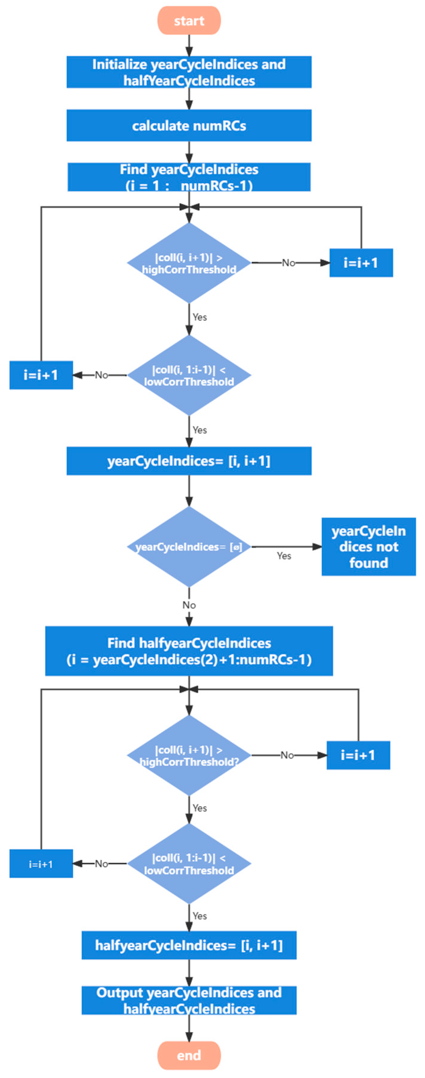
We have improved the reconstruction RC’s ability to find the cycle term by adding the function of automatically finding the annual and semi-annual cycles. This is based on the principle whereby the annual and semi-annual cycles are automatically recognizing by analysis of the correlation of the cycle pairs, by avoiding the subjective selection of a human, and, at the same time, by improving the efficiency. The function’s process is shown in Figure 1.

Figure 1.
Flowchart for the function of automatically finding the annual and semi-annual cycles.
2.2. Principal Component Analysis (PCA)
Let there be m stations in the observation area, with a time span of n days and where n > m, constituting the original coordinate time series matrix . After removing the trend and the seasonal terms, the coordinate residual time series can be obtained. This is delineated into the matrix form , and the covariance array of can be calculated.
Orthogonal decomposition of is as follows:
where is the eigenvector matrix and is the non-zero diagonal matrix consisting of the eigenvalues. Denoting the matrix in terms of yields the following:
namely
In Equation (8), is the kth principal component and is the eigenvector corresponding to the kth eigenvalue.
The contribution of principal components to the original sequence is proportional to their eigenvalues. In order to extract CME signals more intuitively, the eigenvalues are arranged in descending order, and the first q principal components are used to calculate the CME. The subsequent CME calculation formula is as follows:
2.3. Independent Component Analysis (ICA)
Let there be m observatories in the observation area with time series X. The time series consisting of k mutually independent signals y superimposed on each other is represented by the mixing matrix A. The instantaneous mathematical form of a calendar element t is
where is the spatial response of the jth source to the ith observation and is the jth source at time t.
In order to consider the full set of observations, the matrix is of the form
Introducing the unmixing matrix W restores the original signal, namely:
In this paper, tICA is used when extracting CME [14], while the Fast-ICA algorithm is characterized by high computational efficiency and good robustness and so is used to calculate tICA. The contribution of all of the independent components can be obtained by calculating the contribution of all of the independent components, sorting them in descending order and using the first few significant independent components to indicate the most significant signal.
Estimating and from Equations (11) and (12), respectively, the observation network CME is given by
3. Data
3.1. Data Sources
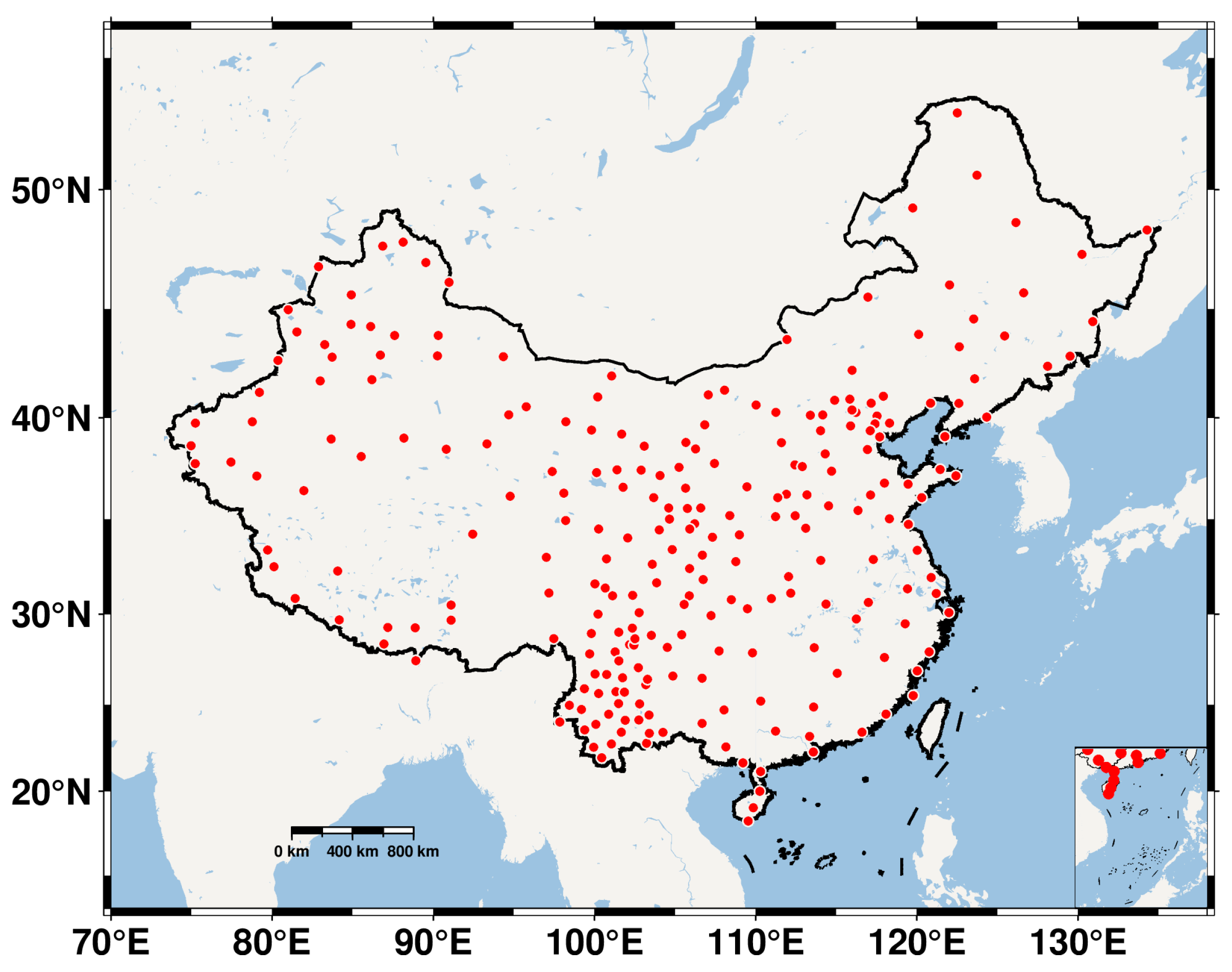
We used the observation data from 260 benchmark stations of the Chinese Mainland Tectonic Environment Monitoring Network (Figure 2), and applied the GPS data post-processing and satellite positioning software GIPSY/OASIS6.0, developed by the Jet Propulsion Laboratory (JPL) of the National Aeronautics and Space Administration (NASA), and adopted the precision single-point positioning data processing strategy [30]. The CMONOC II reference station was rigorously processed on a daily basis to obtain the raw coordinate change time series of each station based on ITRF2020 (Figure 3). Among these, CMONOCII is a nationally integrated geoscience observation network for real-time monitoring and consists of more than 260 reference stations for continuous observation and more than 2000 regional stations for irregular observation. The spatial scale of CMONOCII is about 5000 km, which can be regarded as a large spatial scale, and at the same time accurately reflects the spatial distribution characteristics of CME. The principles of site selection are as follows: (1) the missing rate of site data is less than 20% and (2) the time series of site coordinates span more than 12 years and have high stability. We selected 247 stations in mainland China to form a large spatial scale GPS network, whose time span is from October 2011 to October 2023, and the average missing rate of station data is 4.79%, indicating that it has less of an influence on the experimental results.

Figure 2.
GPS station distribution.
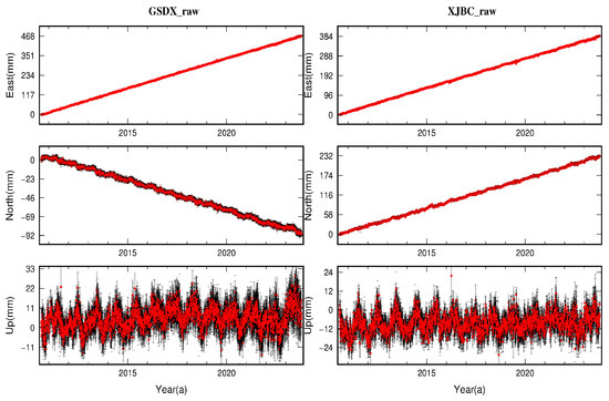
Figure 3.
Original coordinate time series of GSDX and XJBC station (The red dots show the coordinate values and the black lines show the error bars.).
3.2. Acquisition of Residual Time Series
It is common practice to extract CME from residual time series, which are the time series obtained by excluding outliers from the original coordinate time series, interpolating, correcting the step terms, and removing the trend and seasonal terms. GPS residual time series can usually be expressed using Equation (14) [31]:
where is the residual of the observed object; is a single-station coordinate time series; is the time, is the linear rate of change; are the coefficients of the anniversary term; and are the coefficients of the half-anniversary term. The offset correction term is , where is the offset correction value, is the number of the known offset epoch, is the number of offsets, and is the Heaviside step function.
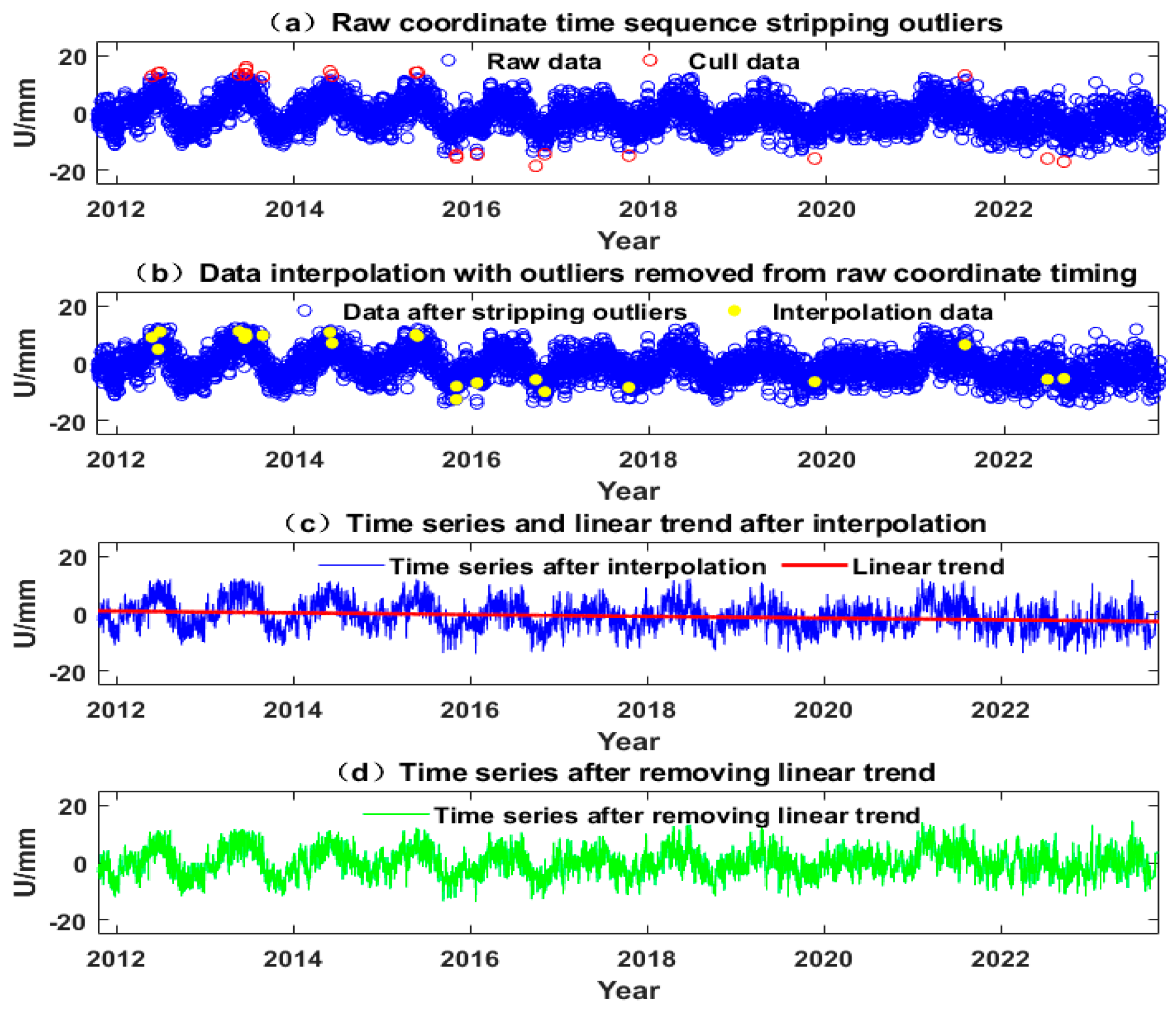
We used the triple-quartile spacing method to remove outliers and used a combination of nearest neighbor interpolation and linear interpolation to interpolate the culled outliers with the original missing data. The least square method was used to fit the trend item on the interpolated data. The results, after removing outlier, interpolation and fitting the trend item in the U direction time series of the GSDH station, are shown in Figure 4. To fit the seasonal terms, we used two methods, LS and improved singular spectrum analysis (ISSA), for the three directions of the SDCY station, as shown in Figure 5. After preprocessing, the outlier, trend, and seasonal terms of the station coordinate time series are effectively eliminated, and a complete residual time series is obtained.
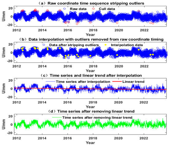
Figure 4.
Results of U-direction timing rejection of outlier, interpolated, and fitted trend terms at GSDH station.
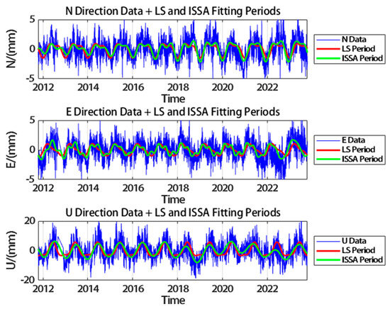
Figure 5.
LS and ISSA seasonal term fitting in E, N, and U directions at the SDCY station.
3.3. Seasonal Term Fitting Results
The seasonal terms in the GPS coordinate time series have typically been expressed as annual and semi-annual term signals by previous authors. These are generally fitted by constant amplitude harmonic function, but the GPS coordinate time series is not a completely fixed amplitude fluctuation, so this paper introduces ISSA for seasonal term fitting, in which the selection of the appropriate window and the interception of the number of principal components are extremely important. Chen et al. [32] and Xiang et al. [33] found that the window selection 2~3a is the most suitable, so this paper chooses the window M = 730. The number of intercepted principal components was judged based on a combination of the variance contribution of the reconstructed RC and the W correlation [34] method, which calculates the correlation by weighting the covariance of the two variables to more accurately reflect their contribution to the correlation. If we seek to identify only the annual and semi-annual term signals, we most achieve this by observing the graph of the weight correlation function, which is mixed with human subjective factors. In order to enable the automatic identification of the annual and semi-annual term signals we add the associated function, which simultaneously avoids the human subjective choice and improves efficiency. As shown in Figure 6, which shows the W correlation of the first 20 orders of reconstructed RCs of the E component of the AHAQ station, the principal components of the adjacent order terms with better correlation are considered period pairs containing the same period [35]. We judge the annual and semi-annual term signals by the correlation of the period pairs, i.e., the first group of adjacent RCs with better correlation (greater than 80%) and with the other RCs that are lower (40%). The second such pair is considered to comprise the annual term signals, and the second such pair is considered to comprise the semi-annual term signals. The annual term signals should be RC1 + RC2 and the semi-annual term signals should be RC5 + RC6, shown in Figure 6. The seasonal terms are fitted using this method for all components of the remaining stations.
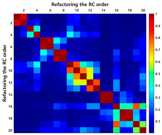
Figure 6.
W correlation of the first 20 orders of reconstructed RC for the E component at AHAQ station.
The results of the seasonal term fitting (Figure 7) can be calculated to show that about 80% of the sites in the N direction using the LS fitting seasonal term have a goodness of fit R2 centered on 0–0.30, while about 80% of the sites using the ISSA fitting seasonal term have a goodness of fit R2 centered on 0–0.43. About 80% of the sites in the E direction using the LS fitting seasonal term had a goodness of fit R2 centered on 0–0.20, while about 80% of the sites using the ISSA fitting seasonal term had a goodness of fit R2 centered on 0–0.37. About 80% of the sites in the U direction using the LS fitting seasonal term had a goodness of fit R2 centered on 0–0.42, while about 80% of the sites using the ISSA fitting seasonal term had a goodness of fit R2 centered on 0–0.50. Comparison of the data shows that fitting the period using ISSA is better in all three directions. Accurately identifying and fitting the period avoids inaccurate CME extraction caused by entering the period component of the original time series into the residuals.
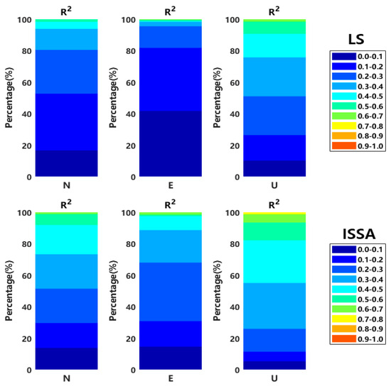
Figure 7.
Comparison of LS and ISSA seasonal term fitting effects.
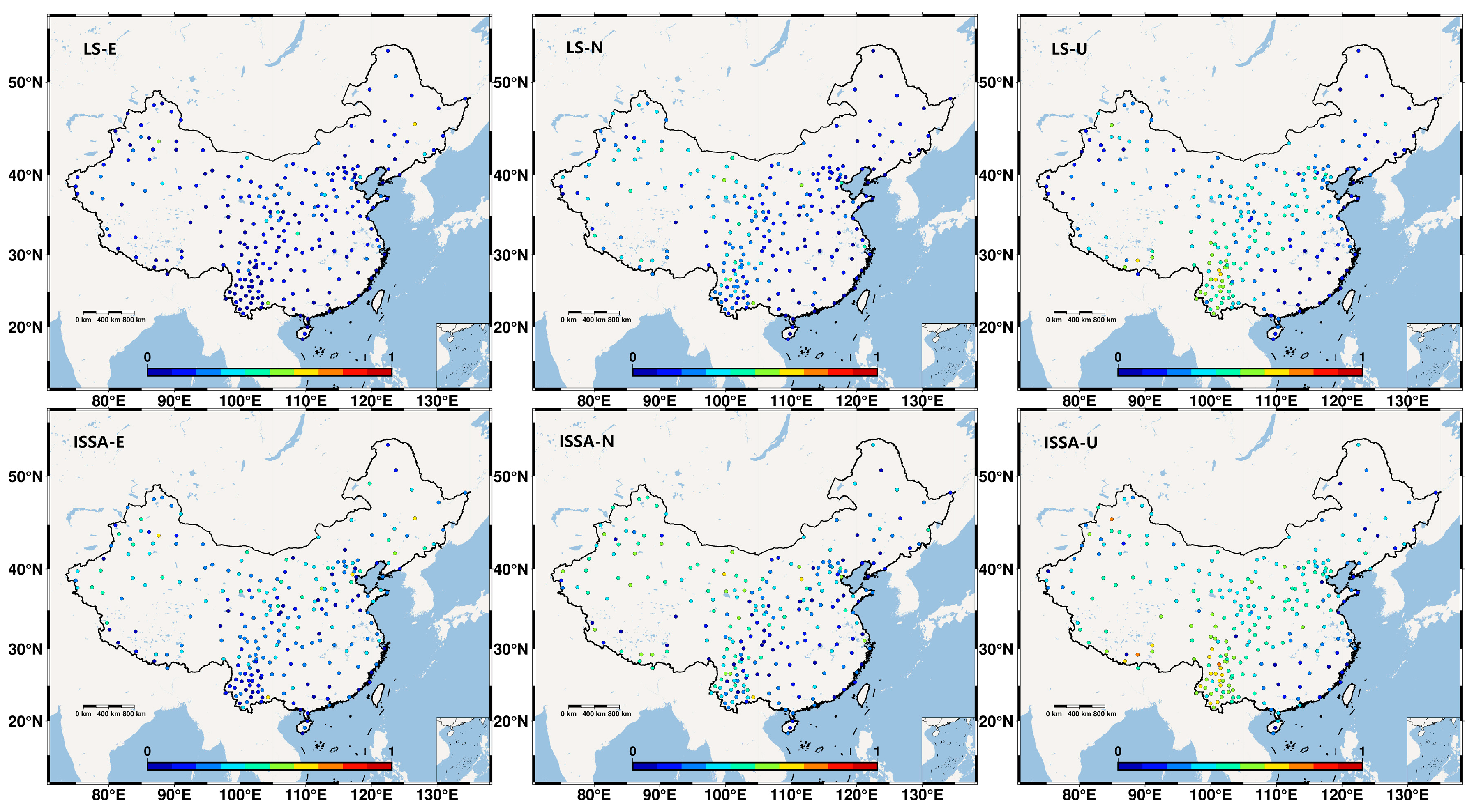
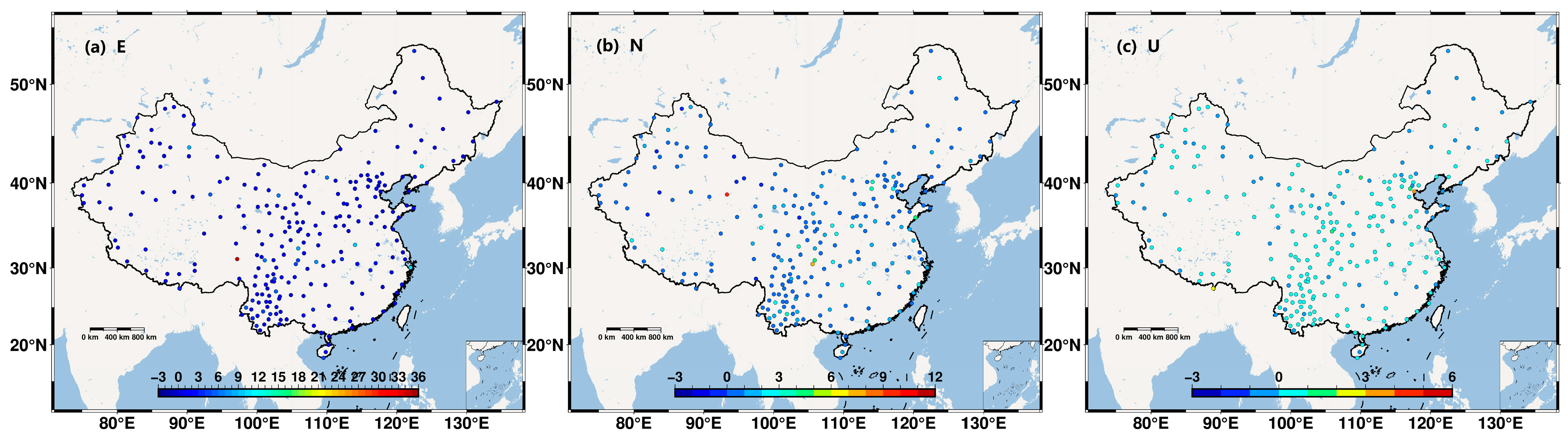
Figure 8 illustrates the magnitude of the goodness of fit R2 for each station in this GPS network when fitting the seasonal term in different directions using the two methods. Both methods show that the U direction fit is better than the N direction fit, which is in turn better than the E direction fit, and the ISSA fit is better than the LS fit in each direction. In the E direction, only 1.62% of sites with LS fitting period were fitted better (>0.40), and Chuandian region was fitted worse; 11.34% of sites with ISSA fitting period were fitted better (>0.40), and Chuandian region was fitted worse. In the N direction, only 6.07% of the sites with LS fitting seasonal term were fitted better (>0.40), with poorer fits in southern and northern China, and 26.72% of the sites with ISSA fitting seasonal term were fitted better (>0.40), with poorer fits in southern and northern China. In the U direction, 24.29% of the sites had a better LS fit period (>0.40), with the best fit in Chuandian region and the worst in the southeast coast, and 44.94% of the sites had a better ISSA fit period (>0.40), with the best fit in Chuandian region and the worst in the southeast coast. Overall, the ISSA fit is better than the LS fit, and therefore ISSA is considered more suitable for fitting seasonal terms to the time series of site coordinates in this study area.
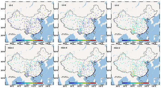
Figure 8.
Distribution of the effects of fitting the LS and ISSA seasonal terms to the time series of stations in the study area.
4. Results of Large Spatial Scale Filtering
4.1. PCA Filtering Results
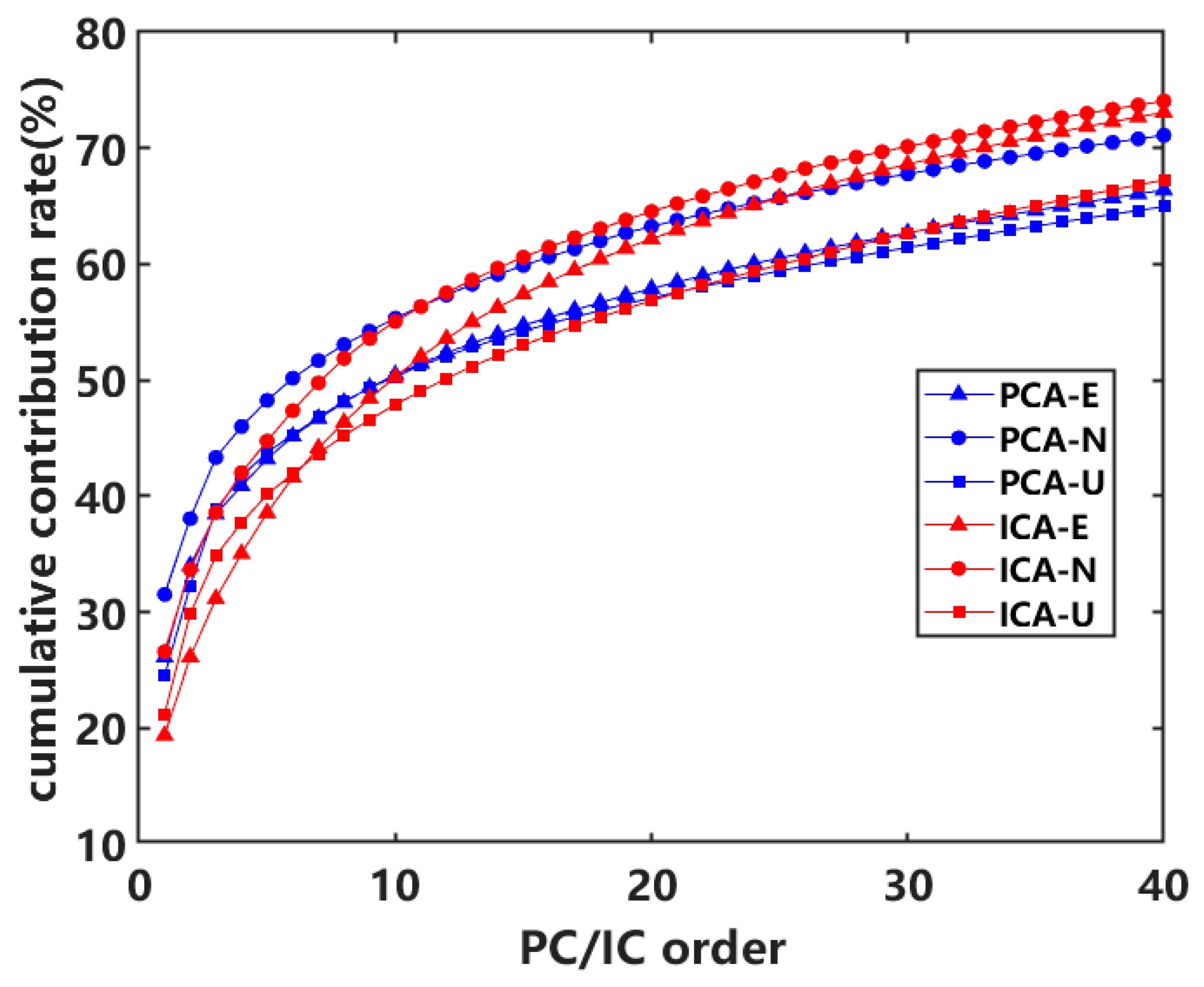
The PCA/ICA filter was applied to the complete residual time series and the cumulative contribution rate (CCR) of PC/IC for the N, E and U components was calculated as shown in Figure 9. The first fifth-order contributions of the residual sequence PCA/ICA are shown in Table 1, and both PCA and ICA show that the sum of the first fifth-order contributions in the N direction is greater than the sum of the first fifth-order contributions in the U direction, which in turn is greater than the sum of the first fifth-order contributions in the E direction. Simply determining the principal components by virtue of the variance contribution ratio leads to the neglect of some PCs with small eigenvalues but significant spatial responses. PCA decomposes the coordinate time series into PCs in the time domain and eigenvectors in the spatial domain (which are normalized to become spatial responses), and CMEs can be represented by the PCs to represent their changes in the time domain, and the spatial responses of the corresponding PCs reveal their spatial distribution characteristics. The SRs of the first five PCs of the E, N, and U components are shown in Figure 10, Figure 11 and Figure 12, where the SRs are the normalized results, and the response value with the largest absolute value is 100%, with blue arrows pointing up to indicate a positive response, and red arrows pointing down to indicate a negative response. Dong et al. [13] have shown that more than 50% of the stations with spatial response values > 25% and whose eigenvalues of the mode are more than 1% of the sum of all the eigenvalues can be considered as common mode. According to the definition of CME by Dong et al. [13], it has been calculated that only PC1 in each direction satisfies its condition, so the CME is extracted using PC1 in each direction for 247 stations, and the average RMSE of the residuals after extracting the CME in the E, N, and U directions decreases by 2.23%, 2.37%, and 0.64%, respectively, which is not ideal for its extraction. A CME is a spatially correlated error, which Ming et al. [15] have argued should be defined based on the spatial distribution characteristics rather than on the magnitude of its variance. Based on this and on Figure 10, Figure 11 and Figure 12, CME was extracted using PC1, PC2, and PC3 in each direction for 247 stations, and the mean value of the residual RMSE was reduced by 4.20%, 4.22%, and 1.30%, respectively. The effect of extracting CME according to the definition of CME proposed by Ming et al. [15] is somewhat improved over the effect of extracting CME proposed by Dong et al. [13], but the effect is still unsatisfactory, so the residual time series are analyzed by Kurtosis analysis, with the results shown in Figure 13. These results show that the probability density of the residual time series does not completely obey the Gaussian distribution. About 99.60% of the E component, 95.95% of the N component, and 72.87% of the U component are super-Gaussian distribution (i.e., the Kurtosis is greater than 0), and the second-order statistical information of the super-Gaussian distributed time series does not fully describe its statistical characteristics. The PCA only uses the second-order statistical information of the data, so we consider the PCA to be inapplicable to the CMONOCII observation network analyzed in this paper. This conclusion is consistent with that obtained by Ming et al. [15].

Figure 9.
Cumulative contribution of PC/IC in the first 40 orders in the N, E, and U directions.

Table 1.
Contributions of the first five orders of the residual series PCA/ICA.

Figure 10.
Spatial response results for the first five PCs of the E component after PCA filtering (arrows indicate the normalized spatial response, blue indicates a positive spatial response and red indicates a negative spatial response).
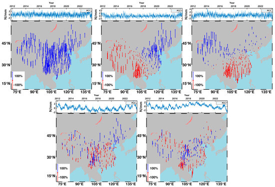
Figure 11.
Spatial response results for the first five PCs of the N component after PCA filtering (arrows indicate the normalized spatial response, blue indicates a positive spatial response and red indicates a negative spatial response).
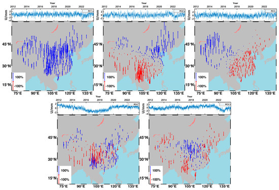
Figure 12.
Spatial response results for the first five PCs of the U component after PCA filtering (arrows indicate the normalized spatial response, blue indicates a positive spatial response and red indicates a negative spatial response).
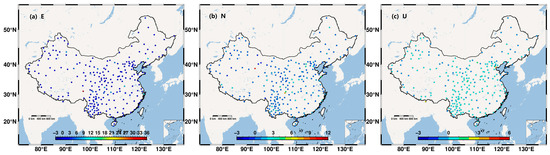
Figure 13.
Results of residual time series Kurtosis analysis.
4.2. ICA Filtering Results
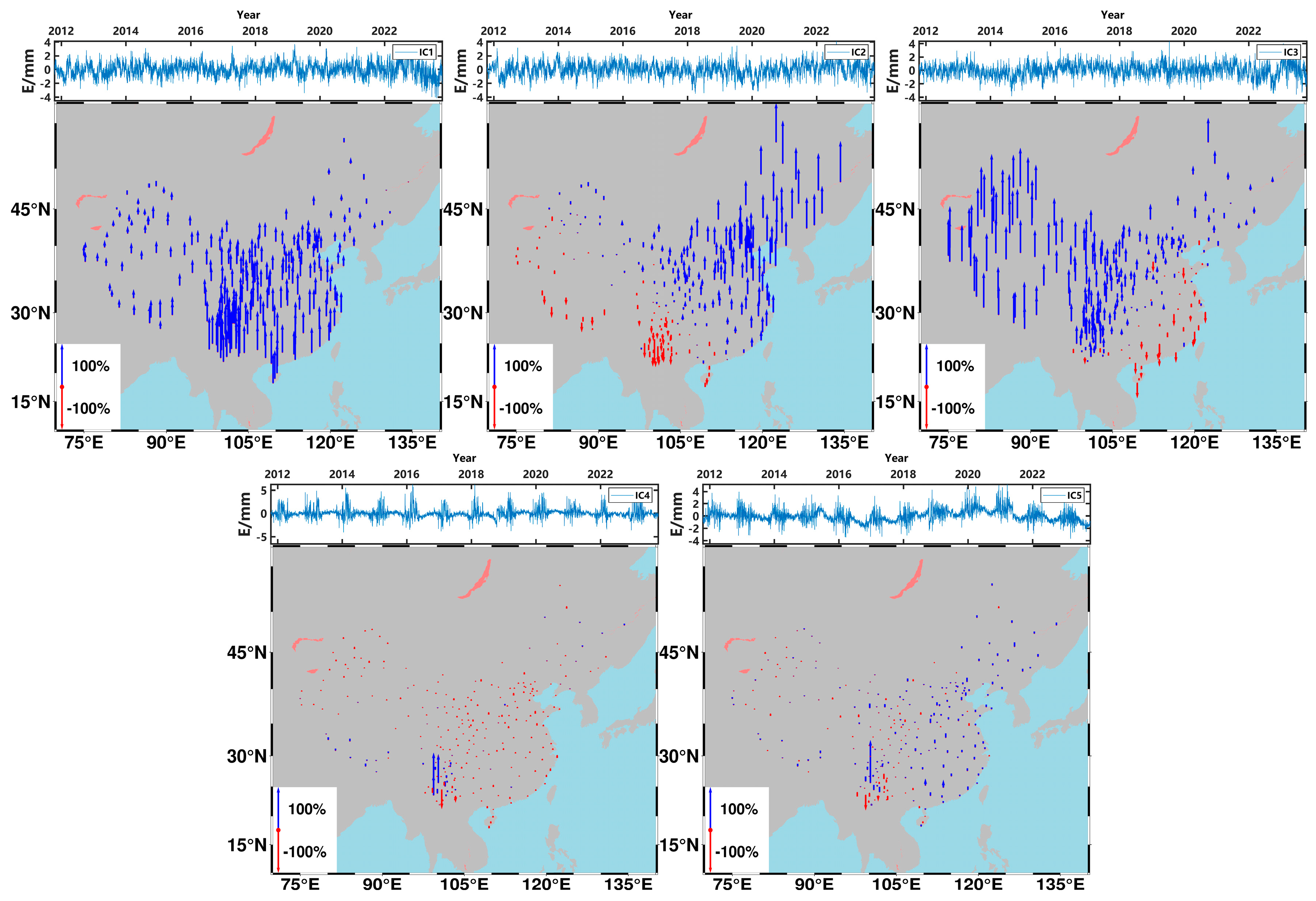
Unlike PCA, ICA, as a blind source signal separation method, can decompose the mixed signal into multiple independent signals and maximize the non-Gaussian components to separate the anomalous signal into independent components. The SR of the first five ICs of the E, N, and U components are shown in Figure 14, Figure 15 and Figure 16, where SR is the result after normalization, and the response value with the largest absolute value is 100%, with blue arrows pointing up to indicate a positive response, and red arrows pointing down to indicate a negative response. According to the definition of CME proposed by Dong et al. [13], it is calculated that only IC1 satisfies its condition in the E direction, and both IC1 and IC2 satisfy their conditions in the N and U directions. As a result, CME is extracted using 247 stations, with IC1 in the E direction and with IC1 and IC2 in the N and U directions, respectively. The RMSEs of the residuals of the extracted CMEs in the E, N, and U directions are mean values that were reduced by 9.60%, 17.08%, and 16.14%, respectively. Meanwhile, according to the ICA-based definition of CME proposed by Ming et al. [15], it is considered that, if an IC has obvious spatial characteristics, then that IC is one of the source signals of the CME. Additionally, based on this definition and on Figure 14, Figure 15 and Figure 16, by using 247 stations in the E and U directions with IC1, IC2, and IC3 to extract CMEs, and by using IC1, IC2, IC3, and IC4 to extract CMEs in the N direction, the average residual RMSE values are reduced by 20.28%, 20.25%, and 25.56%, respectively. Based on these two CME definitions and the results of PCA and ICA, the CME definition and ICA proposed by Ming et al. [15] are more suitable for the extraction of CMEs from the CMONOC II observation network.
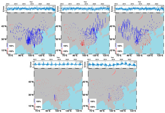
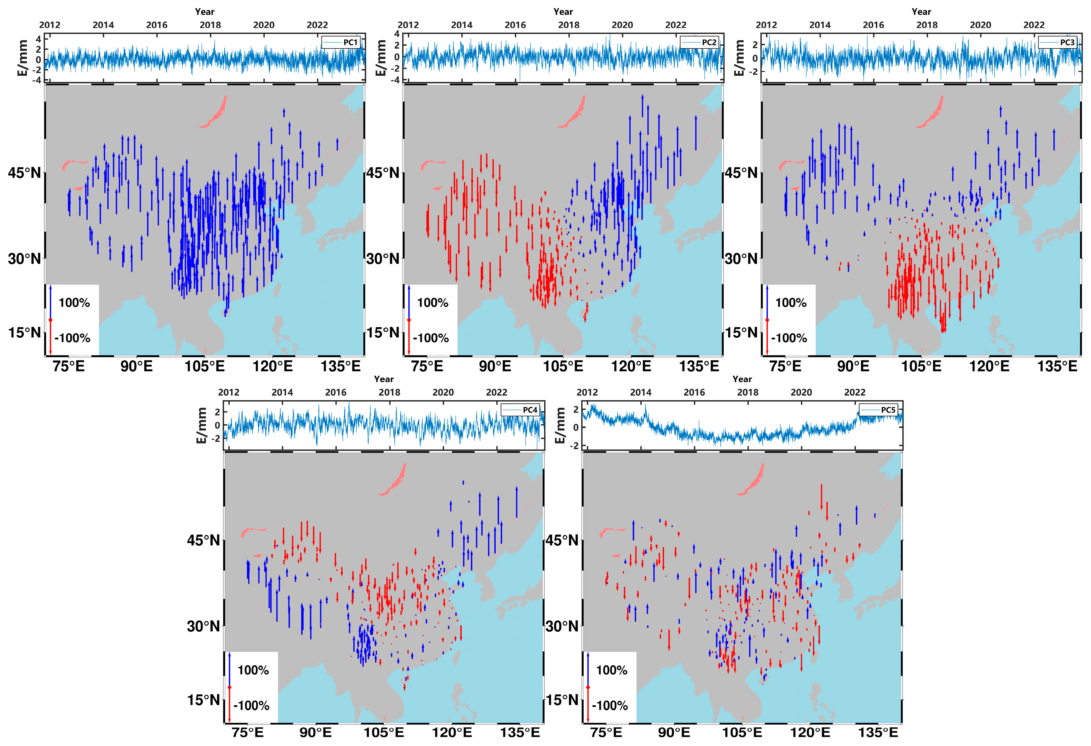
Figure 14.
Results of the spatial response of the first five ICs of the E component after ICA filtering (arrows indicate the normalized spatial response, blue indicates the positive spatial response and red indicates the negative spatial response).
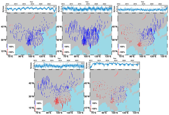
Figure 15.
Results of the spatial response of the first five ICs of the N component after ICA filtering (arrows indicate the normalized spatial response, blue indicates the positive spatial response and red indicates the negative spatial response).
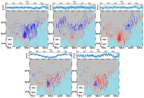
Figure 16.
Results of the spatial response of the first five ICs of the U component after ICA filtering (arrows indicate the normalized spatial response, blue indicates a positive spatial response and red indicates a negative spatial response).
For the SR results, we find that the SR1 of the E component (Figure 14) shows spatial coherence, with larger sizes observed in the center and east and smaller sizes observed in the northeast and west. The SR2 and SR3 show obvious NE–SW or NW–SE asymmetric distributions with respectively opposing signs. SR2 and SR3 show obvious northeast–southwest or northwest–southeast asymmetric distributions with opposite signs, and the sizes of the SRs of the above two modes are smaller at the intersection of the positive and negative regions and larger at the edges, which indicates that there exists a smooth transition zone between the positive and negative regions. SR4 and SR5 indicate that there may be anomalous stations, and that all of these are located in Chuandian region, possibly due to the fact that the signals of some of the stations are affected by the local environment. For the N component (Figure 15), SR1 and SR2 show relatively consistent spatial distributions and the spatial response values in Chuandian region are slightly higher than those in other regions. SR3 is consistent with the spatial distribution of SR2 for the E component, showing an obvious northeast–southwest incomplete symmetrical distribution with opposite signs. SR4 shows an obvious south–north incomplete symmetric distribution with opposite signs, and there is a smooth transition zone between the positive and negative regions of the SRs of the above two modes. SR5 does not show obvious spatial distribution characteristics and local features. For the U component (Figure 16), SR1 is spatially consistent, with the magnitude of SR being smaller in the west and larger in the central east and northeast. SR2 shows a gradual decrease in SR from north to south, with negative responses in Chuandian region, and part of south China. SR3 shows a clear northeast–southwest asymmetric distribution with opposite signs, with the size of SR being smaller at the intersection of positive and negative regions and larger at the edges and with a smooth transition between positive and negative regions. SR2 shows a gradual decrease in SR from north to south, with some areas in Chuandian and South China showing a negative response. SR3 shows an obvious asymmetric distribution from northeast to southwest with opposite signs, with the size of SR being smaller at the intersection of the positive and negative regions and larger at the edges and with a smooth transition zone between the positive and negative regions. SR4 does not show an obvious spatial distribution at all, but local areas will show spatial consistency; for example, Chuandian, eastern South China, Tibetan Plateau, and Xiyu region show spatially positive responses, while most of the stations in northeast China, east North China, Gansu’s surrounding areas, and South Qinghai–Tibet show spatially negative responses. In SR5, the overall spatial distribution also does not show obvious characteristics, but most of the stations in different areas show spatial consistency, with most of the stations in Northeast China, North China, South China, and the Tibetan Plateau showing spatially negative responses, while most of the stations in Chuandian and western Xiyu show spatially positive responses.
5. Results of Sub-Regions Filtering
5.1. Principles of Fine Determination of Active Tectonic Block Regions
Prior research results have shown that the results of regional filtering in small spatial scales are better than those in large spatial scales, but that there is no uniform division standard. For the spatial distribution characteristics of the CMEs shown in the above experiments and for the modern tectonic deformation of the Chinese continent, mainly characterized by tectonic block regions that have active tectonic blocks and, as pointed out by Zhang et al., the relatively uniform movement mode of its geologic unit [29], this paper proposes to divide subregions in accordance with the first-level active tectonic block regions. The active tectonic blocks proposed by Zhang et al. [29] in mainland China are shown in Figure 17a. Here, some stations of the CMONOC II observation network are located in the junction region of two or more tectonic block regions, such as BJSH, BJYQ, NMBT, NMTK, TJBD, and TJBH between the northeast active tectonic block region and the North China active tectonic block region. To this we might add the stations of GSJN and GSDX, which are located in the North China active tectonic block region, the South China active tectonic block region, and the Tibetan Plateau active tectonic block region. We refined the boundaries of the active tectonic block region in mainland China by calculating the spatial response values of the site using ICA and its neighboring tectonic block region. For example, the NXYC site is located between the North China tectonic block region and the Xiyu active tectonic block region, and the spatial responses of the NXYC site in the North China active tectonic block region in the three directions of E, N, and U are calculated to be 67.18%, 51.56%, and 73.99%, respectively, while the spatial responses of the NXYC site in the Xiyu active tectonic block region in the three directions of E, N, and U are 0.65%, 42.82%, and 21.38%, respectively. After comparing the spatial responses of the NXYC site in all three directions in the North China active tectonic block region, we found them to be greater than the spatial responses in the Xiyu active tectonic block region. This indicates that the NXYC site should be assigned to the North China active tectonic block region. The results of the spatial response calculation of some sites are shown in Table 2, and all inter-plot sites are classified into adjacent plots according to the size of the spatial response value with the adjacent plots. The first-level active tectonic-block region of the Chinese mainland is shown in Figure 17b, after the refinement of the determination. Here, the Chinese mainland is divided into six regions, namely, Chuandian, Northeastern, Northern China, Southern China, Tibetan Plateau, and Xiyu.
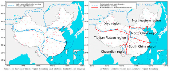
Figure 17.
Distribution of active tectonic block regions in mainland China and the results of the refinement of determination(The red dots represent GPS stations in the figure.).
Table 2.
Results of spatial response calculations for selected sites.
5.2. Comparison of Large Spatial Scale Region and Sub-Regions Filtering Effects
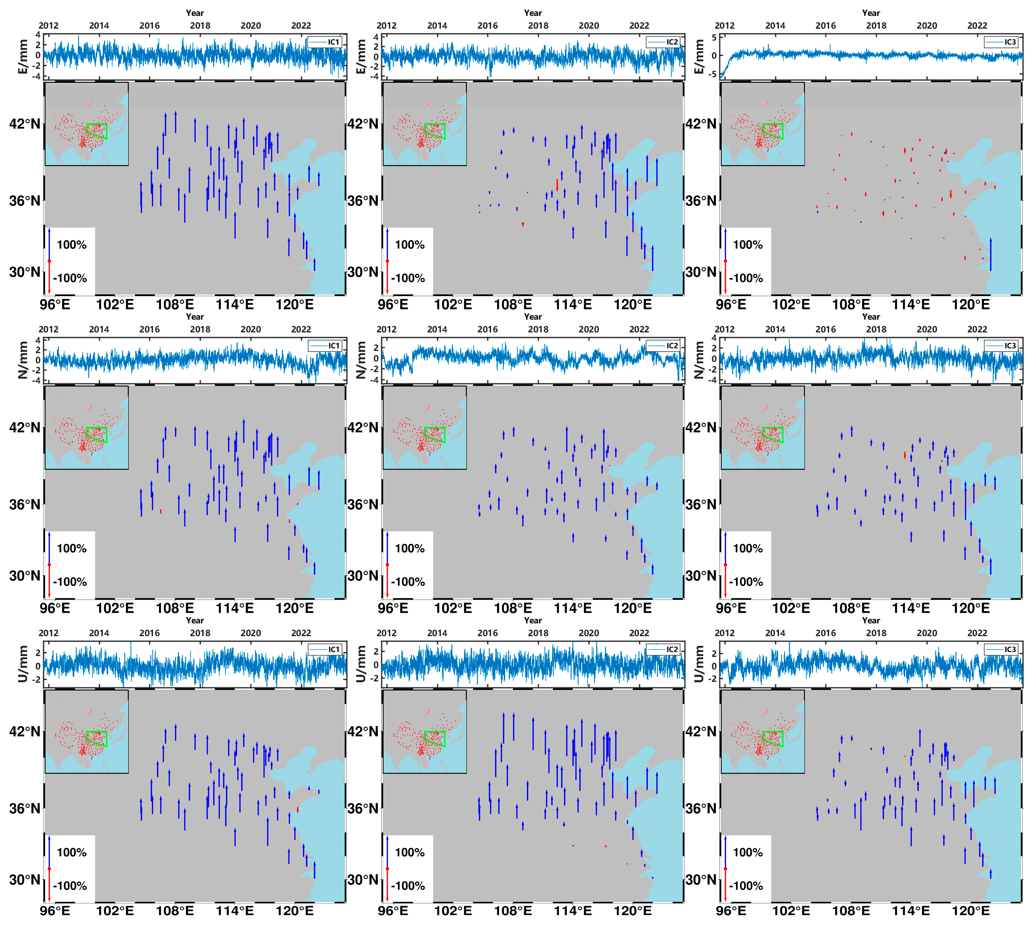
The residual time series of CMONOC II stations in each tectonic block region are filtered by ICA, and the CMEs are extracted according to the criterion that ICs with obvious spatial characteristics are one of the source signals of the CMEs. Among the SR maps, those of the North China region are shown in Figure 18. These are also characterized by obvious spatial distributions, with the E component for SR2 and the N component for SR3 exhibiting a gradual decrease of the SR from east to west, the U component for SR2 exhibiting a gradual decrease in SR from north to south, and the N component for SR2 and the U component for SR3 each exhibit a northwest–southeast symmetric distribution with the same sign, with a gradual increase in SR from both sides to the center. According to the definition of CME by Ming et al. [15], a CME is extracted by taking several orders of IC in the E, N, and U directions for each active tectonic block region GPS network, as shown in Table 3. According to the IC selection in Table 3, the CME extraction is performed on the residual sequences of GPS networks in each region, and the results are shown in Table 4. Here, the three directions of E, N, and U show that the residual time series RMSE reduction ratio of the northeastern and western plots is higher than the average value for the other plots. The RMSE reduction ratio of the residual time series of the Chuandian region is lowest, and is much lower than the average value. The spatial scales of each of the active tectonic block regions in Table 4 are smaller than the overall spatial scale, but the filtering results of the E, N and U components of the GPS network in Chuandian region are poorer than the overall filtering effect. The filtering results of the N component of the GPS network in the North, South and Tibetan Plateau regions are also poorer than the overall filtering result. This is contrary to some of the existing research results, indicating that the conclusion that the regional filtering results at small spatial scales are better than those at large spatial scales does not apply to all of the stations of the CMONOC II observation network in this study, but only to some areas. The reason for the poor filtering results in Chuandian region may be due to the poor fitting of the seasonal terms in the original coordinate time series in this region, which does not accurately remove the seasonal terms, or the filtering results may be inaccurate due to the presence of more anomalous stations in this region. Additionally, this may be due to the fact that this region contains many secondary active tectonic block regions, which has complicated movements among the secondary active tectonic block regions. By separating and removing CME results using ICA filtering for the large spatial scale GPS network and six small spatial scale GPS networks divided according to active tectonic block regions (Table 4), we find that the effect of extracting CME in subregions improves by 29.16%, 5.44%, and 39.84% in the three directions of E, N, and U, respectively, when compared with the overall extraction. The experimental results prove that the CMONOC II observation network, by dividing the sub-regions according to the first-level active tectonic block regions in mainland China, is an effective and feasible method by which to extract CMEs; therefore, for the study of CME removal in the GPS network in mainland China, one should consider whether the study area comprises cross tectonic blocks and one should try to choose the same tectonic blocks for the study.
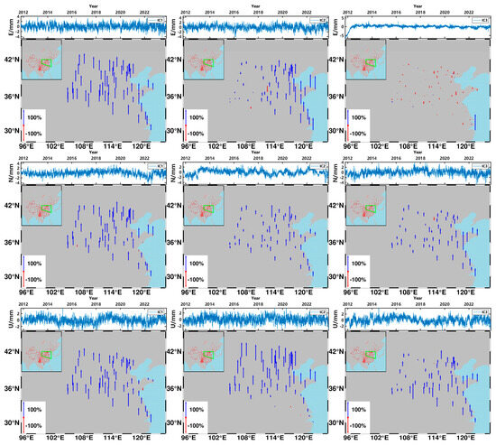
Figure 18.
Spatial response results for the first three ICs of the E, N, and U components after ICA filtering of the residual time series at the North China region site (arrows indicate the normalized spatial response, blue indicates a positive spatial response, and red indicates a negative spatial response).
Table 3.
GPS network in different directions and different IC selections for each active tectonic block region.
Table 4.
Percentage of reduction in overall and segmented RMSE averages.
6. Discussion
The GPS coordinate time series can be made more accurate by eliminating CME. CME is a kind of spatially related error in GPS time series, and the larger the spatial distance the weaker the CME. The effect of CME extraction in small areas should be better than that in large areas. Considering the effect of mutual motion between active blocks on CME and the weaker correlation of the residual time series with the increase of distance, we propose to extract CME by region for mainland China.
In this paper, we find that ISSA fits the seasonal terms better than LS, which can be clearly seen in Figure 6. However, for mainland China, the ISSA method of fitting seasonal terms does not work well in all areas; for example, the N and E directions in Chuandian and Yunnan are not ideal. For Chuandian region, we can try multiple seasonal term fitting methods to determine the optimal fitting method. In the article, we used PCA and ICA to spatially filter the large spatial scale GPS network and found that the PCA filtering effect is not ideal and that ICA filtering can effectively extract the CMEs in the GPS network. We analyzed the Kurtosis analysis of the residual time series and found that the residual time series do not fully conform to the Gaussian distribution, which can explain the reason for the unsatisfactory effect of PCA filtering. The results of Kurtosis analysis are consistent with Ming et al. [15]. Subsequently, we can try to improve PCA or ICA to in turn improve the filtering effect. We extracted the CME results in chunks, as shown in Table 4, and found that the filtering effect in Chuandian is worse than the overall filtering effect. We think this may be because the active tectonic block region of Chuandian is more special. One reason for this is that the seasonal terms are poorly fitted in the Chuandian region, which makes the obtained residual time series inaccurate, another reason is that there are more anomalous stations in the Chuandian region, which is consistent with Miao et al. [6]. Yet another reason might be the fact that the Chuandian region contains many secondary tectonic block regions. In conclusion, the CME extraction in Chuandian region is still to be further studied. In Table 4, by comparing the overall residual time series RMSE reduction ratio with the average value of the residual time series RMSE reduction ratio of the sub-block extraction, there are improvements in all three of the directions, which proves that the GPS network of the Chinese mainland is effective at extracting the CMEs according to the division of first-level active tectonic block regions of the Chinese mainland into sub-regions.
There are some limitations of this study, as follows: (1) we did not exclude the outlier sites; (2) we did not further analyze the extracted CMEs, though subsequent analysis of the CME cycle can be undertaken and this will help to analyze the CME causes; and (3) we did not perform a noise analysis to clarify how the noise model changes.
7. Conclusions
The CME is one of the main error sources in a GPS area network, and will have a significant impact on its coordinate time series. It has been shown that the seasonal term fitting effect will have an impact on the CME extraction effect, we used LS and ISSA to extract the seasonal terms, and the experimental results show that the ISSA-based extraction of the seasonal terms of the coordinate time series is more effective. Effective extraction of seasonal terms can prevent part of the unfitted seasonal term signals from entering the residual time series, which in turn leads to inaccurate CME extraction results.
More accurate time series of residual coordinates can be obtained based on ISSA. Spatial filtering can effectively extract and remove CME and can improve the accuracy of GPS coordinate time series. For CMONOC II, there is a lack of research with which to prove which spatial filtering can remove CME most effectively. In this paper, we compare two filtering methods, PCA and ICA, and the results show that PCA filtering is not effective in removing CME. We perform a Kurtosis analysis on the residuals of the coordinate time series and find that the probability density of the residual time series does not completely obey the Gaussian distribution and that most of the site time series of the three components are super-Gaussian. PCA uses only the second-order statistical information of the data, and it cannot completely describe the statistical characteristics of the time series with super-Gaussian distributions; therefore, we consider PCA to be inapplicable to the CMONOC II observation network analyzed in this paper. ICA can take into account the higher-order statistical information. Using ICA to filter the residual time series, their average RMSE in the three directions of E, N, and U are reduced by 20.28%, 20.25%, and 25.56%, respectively. This proves that ICA can effectively remove the CME of the coordinate time series of the CMONOC II observation network. For the extracted CME sequences, it can be found that these sequences have obvious spatial distribution characteristics and that the SRs of different components will show an incomplete symmetric distribution of northeast–southwest or northwest–southeast with opposite signs. Furthermore, the size of the modal SRs is smaller at the intersection of the positive and negative regions and larger at the edges, with a smooth transition zone between the positive and negative regions.
Based on the spatial distribution characteristics of CME, we propose a sub-region division method for the CMONOC II observation network, i.e., dividing it into six sub-regions by the boundary of the first-level active tectonic block regions in mainland China. The results show that the effect of extracting CME by sub-regions is 29.16%, 5.44%, and 39.84% higher than that of the overall extraction in the three directions of ENU, respectively. This proves that ours is an effective and feasible method with which to extract CME, whereby we divide the CMONOC II observation network into sub-regions according to the first-level active tectonic block regions in mainland China.
Author Contributions
Data curation: B.B. and G.X.; formal analysis: B.B., P.M. and C.L.; funding acquisition: G.X. and F.S.; methodology: B.B., G.X. and P.M.; writing—original draft: B.B.; writing–review and editing: B.B., G.X. and F.S. All authors have read and agreed to the published version of the manuscript.
Funding
National Natural Science Foundation of China (42374040); Innovation Fund Designated for Graduate Students of ECUT (YC2023-S584).
Data Availability Statement
In view of confidentiality and the need for permission from the authors, data and materials will be available on request.
Acknowledgments
We are grateful for the GPS observations from the China Earthquake Administration.
Conflicts of Interest
Author Genru Xiao was employed by the company Nanjing Zhixing Map Information Technology Co., Ltd. The remaining authors declare that the research was conducted in the absence of any commercial or financial relationships that could be construed as a potential conflict of interest.
References
- Sun, H.; Xu, J.; Jiang, L.; Liu, G.; Zheng, Y.; Yan, H.; bao, L.; Hu, X.; Zhou, J. Research progress of the modern geodesy with its application in Geosciences. Bull. Natl. Nat. Sci. Found. China 2018, 32, 131–140. [Google Scholar] [CrossRef]
- Bo, W.-J. Mainly relative deformation features on China continent revealed by GPS and researches on strong earthquake activities. Prog. Geophys. 2013, 28, 599–606. [Google Scholar] [CrossRef]
- Gan, W.; Li, Q.; Zhang, R.; Shi, H. Construction and Application of Tectonic and Environmental Observation Network of China’s mainland. J. Eng. Stud. 2012, 4, 324–331. [Google Scholar]
- Li, Z.; Yue, J.P.; Li, W.; Lu, D.K. Investigating mass loading contributes of annual GPS observations for the Eurasian plate. J. Geodyn. 2017, 111, 43–49. [Google Scholar] [CrossRef]
- Bock, Y.; Wdowinski, S.; Fang, P.; Zhang, J.; Williams, S.; Johnson, H.; Behr, J.; Genrich, J.; Dean, J.; van Domselaar, M.; et al. Southern California Permanent GPS Geodetic Array: Continuous measurements of regional crustal deformation between the 1992 Landers and 1994 Northridge earthquakes. J. Geophys. Res. Solid Earth 1997, 102, 18013–18033. [Google Scholar] [CrossRef]
- Miao, P.; Xiao, G.; Wang, S.; Zhang, K.; Bai, B.; Guo, Z. Effects of different seasonal fitting methods on the spatial distribution characteristics of common mode errors. Front. Earth Sci. 2023, 11, 1176241. [Google Scholar] [CrossRef]
- Li, Z.; Jiang, W.; Liu, H.; Qu, X. Noise Model Establishment and Analysis of IGS Reference Station Coordinate Time Series inside China. Acta Geod. Et Cartogr. Sin. 2012, 41, 496–503. [Google Scholar]
- Fan, Y.; Wang, H.; Huang, S.; Lu, Q. Analysing the nonlinear motion characteristics of IGS tracking stations using wavelets. Eng. Surv. Mapp. 2014, 23, 5–8. [Google Scholar] [CrossRef]
- Zhang, S.; Li, Z.; He, Y.; Hou, X.; He, Z.; Wang, Q. Extracting of periodic component of GNSS vertical time series using EMD. Sci. Surv. Mapp. 2018, 43, 80–84. [Google Scholar]
- Hu, A.; Wang, T.; Guan, Y.; Yang, Z. Yunnan region vertical GPS time series periodic signal extraction based on SSA. Sci. Surv. Mapp. 2021, 46, 33–40. [Google Scholar] [CrossRef]
- Shu, Y.; Hua, X.; Min, Y.; Teng, H.; Wu, S. Comparison of Common Mode Error Separation Methods for GPS Coordinate Time Series and Their Influences on Noise Model Establishment. J. Geomat. 2023, 48, 20–24. [Google Scholar]
- Márquez-Azúa, B.; DeMets, C. Crustal velocity field of Mexico from continuous GPS measurements, 1993 to June 2001: Implications for the neotectonics of Mexico. J. Geophys. Res. 2003, 108, 2450. [Google Scholar] [CrossRef]
- Dong, D.; Fang, P.; Bock, Y.; Webb, F.; Prawirodirdjo, L.; Kedar, S.; Jamason, P. Spatiotemporal Filtering Using Principal Component Analysis and Karhunen-Loeve Expansion Approaches for Regional GPS Network Analysis. J. Geophys. Res. Solid Earth 2006, 111, B03405. [Google Scholar] [CrossRef]
- Ming, F.; Yang, Y.; Zeng, A. Analysis and Comparison of Common Mode Error Extraction Using Principal Component Analysis and Independent Component Analysis. J. Geod. Geodyn. 2017, 37, 385–389. [Google Scholar]
- Ming, F.; Yang, Y.; Zeng, A.; Zhao, B. Spatiotemporal filtering for regional GPS network in China using independent component analysis. J. Geod. 2017, 91, 419–440. [Google Scholar] [CrossRef]
- Hu, L.; Zhou, Y.; Wang, W. Study on the extraction of common-mode errors in CMONOC. Sci. Surv. Mapp. 2019, 44, 37–42. [Google Scholar] [CrossRef]
- Wang, F.; Dong, D.; Zhang, P.; Sun, Z.; Zhang, Q. Common Mode Error Analysis Based on GPS Station of Chinese Mainland. Earthq. Res. China 2020, 36, 843–856. [Google Scholar]
- Liu, X.; Gao, E.; Luo, Y.; Fu, B. Analysis of Coordinate Time Series of CMONOC GNSS Fiducial Stations Using Principal Component Analysis. J. Geod. Geodyn. 2021, 41, 43–48. [Google Scholar] [CrossRef]
- Wang, H.; Li, W.; Shu, C.; Shum, C.K.; Li, F.; Zhang, S.; Zhang, Z. Assessment of spatiotemporal filtering methods towards optimising crustal movement observation network of China (CMONOC) GNSS data processing at different spatial scales. All Earth 2022, 34, 107–119. [Google Scholar] [CrossRef]
- Wang, J.; Zhou, X.; Zhu, Z.; Liang, L. Research on Elimination of Common Mode Error in Large-Scale GPS Networks. J. Geod. Geodyn. 2018, 38, 78–82. [Google Scholar]
- Xie, S.; Pan, P.; Zhou, X. Research on Common Mode Error Extraction Method for Large—Scale GPS Network. Geomat. Inf. Sci. Wuhan Univ. 2014, 39, 1168–1173. [Google Scholar]
- Yang, B.; Jim, W.; Liu, Z.; Liang, H.; Zhu, S. Identification of common mode error in large spatial domain of GNSS by multi-core function method. J. Geomat. Sci. Technol. 2014, 31, 127–132. [Google Scholar]
- Kreemer, C.; Blewitt, G. Robust estimation of spatially varying common-mode components in GPS time-series. J. Geod. 2021, 95, 95. [Google Scholar] [CrossRef]
- Liu, B.; Dai, W.; Peng, W.; Meng, X. Spatiotemporal analysis of GPS time series in vertical direction using independent component analysis. Earth Planets Space 2015, 67, 189. [Google Scholar] [CrossRef]
- Liu, B.; King, M.; Dai, W. Common mode error in Antarctic GPS coordinate time-series on its effect on bedrock-uplift estimates. Geophys. J. Int. 2018, 214, 1652–1664. [Google Scholar] [CrossRef]
- Serpelloni, E.; Faccenna, C.; Spada, G.; Dong, D.; Williams, S.D. Vertical GPS ground motion rates in the Euro-Mediterranean region: New evidence of velocity gradients at different spatial scales along the NubiaEurasia plate boundary. J. Geophys. Res. Solid Earth 2013, 118, 6003–6024. [Google Scholar] [CrossRef]
- Yuan, P.; Jiang, W.; Wang, K.; Sneeuw, N. Effects of spatiotemporal filtering on the periodic signals and noise in the GPS position time series of the crustal movement observation network of China. Remote Sens. 2018, 10, 1472. [Google Scholar] [CrossRef]
- Wu, S.; Nie, G.; Liu, J.; Wang, K.; Xue, C.; Wang, J.; Li, H.; Peng, F.; Ren, X. A sub-regional extraction method of common mode components from IGS and CMONOC stations in China. Remote Sens. 2019, 11, 1389. [Google Scholar] [CrossRef]
- Zhang, P.; Deng, Q.; Zhang, G.; Ma, J.; Gan, W.; Min, W.; Mao, F.; Wang, Q. Strong seismic activity and active tectonic-blocks region in mainland China. Sci. China Ser. D-Earth Sci. 2003, 33, 9. (In Chinese) [Google Scholar] [CrossRef]
- Liang, S. Three-dimensional Velocity Field of Present-day Crustal Motion of the Tibetan Plateau Inferred from GPS Measurements. Ph.D. Thesis, Institute of Geology, China Earthquake Administration, Beijing, China, 2014. [Google Scholar]
- Nikolaidis, R. Observation of Geodetic and Seismic Deformation with the Global Positioning System. Ph.D. Thesis, University of California, Los Angeles, CA, USA, 2002. [Google Scholar]
- Chen, Q.; van Dam, T.; Sneeuw, N.; Collilieux, X.; Weigelt, M.; Rebischung, P. Singular spectrum analysis for modeling seasonal signals from GPS time series. J. Geodyn. 2013, 72, 25–35. [Google Scholar] [CrossRef]
- Xiang, Y.; Yue, J.; Li, Z. Joint analysis of seasonal oscillations derived from GPS observations and hydrological loading for mainland China. Adv. Space Res. 2018, 62, 3148–3161. [Google Scholar] [CrossRef]
- Hassani, H. Singular spectrum analysis:methodology and comparison. J. Data Sci. 2007, 5, 239–257. [Google Scholar] [CrossRef]
- Xie, G.; Tao, T.; Ma, M.; Hu, S. Analysis of spatial and temporal variation of groundwater storage in Anhui Province using GRACE satellite. J. Hefei Univ. Technol. Nat. Sci. 2024, 47, 367–372+378. [Google Scholar]


Disclaimer/Publisher’s Note: The statements, opinions and data contained in all publications are solely those of the individual author(s) and contributor(s) and not of MDPI and/or the editor(s). MDPI and/or the editor(s) disclaim responsibility for any injury to people or property resulting from any ideas, methods, instructions or products referred to in the content. |
© 2024 by the authors. Licensee MDPI, Basel, Switzerland. This article is an open access article distributed under the terms and conditions of the Creative Commons Attribution (CC BY) license (https://creativecommons.org/licenses/by/4.0/).