Abstract
High-frequency (HF) radar plays a crucial role in the detection of far-range, stealth, and high-speed targets. Nevertheless, the echo signal of such targets typically exhibits a low signal-to-noise ratio (SNR) and significant amplitude fluctuations because their radar cross-section (RCS) accounting for the HF band is in the resonance region. While enhancing detection performance often requires long-time integration, existing algorithms inadequately consider the impact of amplitude fluctuation. In response to this challenge, this article introduces an improved approach based on coherent and non-coherent integration. Initially, coherent integration, employing the generalized Radon Fourier transform (GRFT), is utilized to derive a candidate detection set of targets’ range–time trajectories. This involves a joint solution for range migration (RM) and Doppler frequency migration (DFM) through a multi-parameter motion model search. Subsequently, the removal of low SNR pulses, followed by non-coherent integration, is implemented to mitigate amplitude fluctuation, referred to as Amplitude Fluctuation Suppression (AFS), and refine the detection outcomes. Both simulation and experiment results are provided to prove the effectiveness of the proposed AFS-GRFT algorithm.
1. Introduction
High-frequency (HF) radar is well-known for its over-the-horizon (OTH) property in detecting far-range stealth targets via either surface wave [1,2] or sky wave propagation methods [3,4], including both low-speed sea surface vessels and high-speed airborne targets. Compared with microwave radars, HF radar has advantages in defeating the low-observability techniques for reducing the radar cross-section (RCS) of targets [5]. Nevertheless, the detection of high-speed targets with HF radar is still challenging. On one hand, the serious range migration (RM) and Doppler frequency migration (DFM) caused by the substantial spreading of echo signal across the range and Doppler frequency dimensions limit the integration length and gain [6]. On the other hand, since the RCS of aircraft at HF band is in the resonance region, the corresponding RCS fluctuation with time can be up to more than 20 dB, which further deteriorates the integration performance. The situation is even worse for the compact HF radar system [7] which employs a low-gain antenna and a low transmitting power.
In frequency modulation continuous waveform (FMCW) radar, the range–Doppler processing typically assumes that the target’s radial range change within a period of coherent integration time (CIT) is less than the radar’s range resolution. Then, the target’s radial velocity can be estimated from its phase variation across sweeps through Fourier transform. In this case, the target signal appears as a spike on the range–Doppler plane, and it can be detected through the moving target detection (MTD) algorithm. However, for high-speed targets, long-time integration can no longer be achieved through Fourier transform due to RM and DFM. To address this issue, many efforts have been made to correct different kinds of RM and DFM in the past decade. The basic idea is to accumulate the signal energy along the target’s range–time variation curve, in either a coherent or non-coherent manner. The key is to find an appropriate motion model to match the target’s maneuvering characteristic. The target’s radial range can be represented as a function of time according to Taylor series expansion. Higher order corresponds to more complex maneuverability and higher computation complexity. Generally, a model order less than or equal to three accounts for most cases.
- First-order motion: The first-order Taylor series model is used to express motion with constant radial speed, in which case only RM occurs and DFM does not exist. Typical methods include keystone transform (KT) [8,9,10], Radon Fourier transform (RFT) [11], axis rotation moving target detection (AR-MTD) [12], etc. The KT eliminates RM by re-scaling the slow time axis. The RFT corrects RM via joint two-dimensional searching for the target’s range and speed. The AR-MTD method eliminates RM by rotating the echo locations and achieving energy integration via Fourier transform.
- Second-order motion: The second-order model is used to express motion with constant acceleration, generating second-order RM and first-order DFM. The second-order KT (SKT) [13] can correct RM, and the fractional Radon transform (FRFT) can eliminate DFM. Hence, the combined SKT-FRFT was proposed [14]. This method is computationally efficient but limited in performance compared with simultaneous RM-DFM correction algorithms, such as Radon FRFT (RFRFT) [15], Radon linear canonical transform (RLCT) [16], and Radon Lv’s distribution (RLVD) [17].
- Third-order motion: Similarly, the third-order model corresponds to motion with a constant radial jerk, which will cause additional third-order RM and second-order DFM. The solution can be extended from the first- and second-order cases. For example, RFRFT was extended to the Radon-fractional ambiguity function (RFRAF) by employing a long-time instantaneous autocorrelation function [18]. Xu et al. [19] proposed the generalized RFT (GRFT) method based on RFT by introducing multi-dimensional joint searching. Theoretically, GRFT can apply to arbitrary motion types by adding more search parameters, but the computation complexity increases exponentially with the number of parameters. Fast calculation methods of GRFT [20] have been developed.
By replacing the ergodic search with an iterative adjacent cross-correlation operation, the adjacent cross-correlation function (ACCF) method [21] achieves a very high computation efficiency, but its motion detection accuracy is much lower than GRFT under low SNR conditions. Moreover, an approach combining the generalized KT (GKT) and the generalized de-chirp process (GDP) can also significantly reduce the computation complexity. However, the performance is limited by the Doppler ambiguity issue.
Nevertheless, the above-mentioned methods do not involve the target fluctuations issue, which is usually caused by the variation in RCS with viewing angle and leads to the drop in signal correlation as well as gain loss [22]. A hybrid integration detector based on segmentation was proposed to detect the moderately fluctuating Rayleigh targets in [23], wherein the CIT period is divided into several segments and an appropriate segment length is required to ensure that the signal within each segment is correlated. Then, coherent integration is carried out for each segment, and non-coherent integration is employed to combine all the segments. Its performance is susceptible to the segment length, particularly under low SNR conditions. A segment searching method has been proposed in [24] to determine the optimal segment length, and it was verified using millimeter wave radar data.
During the past decades, the application of long-time integration in HF radar has been much less reported than that in microwave radar. Khan and Power [2] presented experimental results of aircraft detection and tracking using an HF radar with a peak power of 16 kW. Matched filtering in terms of velocities and accelerations has been employed to compensate for RM and DFM, which is similar to GRFT. In [25], the integration time was increased by reducing the sweeping width, which actually did not involve the effect of RM and DFM. Furthermore, a coherent phase-coded pulse train waveform was presented to solve the issue of range–Doppler coupling caused by high-speed target movement [26]. Zvonkovskaya et al. [27] divided the long HF radar data into multiple short segments to avoid RM and DFM within each segment. This method carried out detection within each segment and achieved tracking among segments, which does not exploit long-time integration and thus is limited in low-SNR conditions. In summary, it is challenging to directly apply the previous methods to HF radar because its signal amplitude fluctuation is more dramatic than that of microwave radar.
Inspired by previous work, an improved method combining coherent and non-coherent long-time integration is proposed in this article to address RM and DFM as well as the SNR fluctuation issues in high-speed target detection with HF radar. The two-stage strategy is designed to refine the detection probability and false alarm rate, respectively. At the first stage, GRFT is used to extract target trajectories on the range–time plane. By employing a high false alarm rate threshold, the potential targets with low SNR are identified. Second, false alarms will be refined by applying the amplitude fluctuation suppression (AFS) operation to the SNR-fluctuated targets. Specifically, for each candidate trajectory, the pulses with very low SNR will be identified and removed and then non-coherent integration will be conducted on the remaining pulses. The rest of this article is organized as follows. Section 2 introduces the signal model and outlines the existing problems. Section 3 describes the principle and implementation steps of the proposed AFS-GRFT method. In Section 4 and Section 5, the simulation and experimental results are used to examine the validity and effectiveness of the proposed method, respectively. Section 6 presents the conclusion and ongoing work.
2. Problem Formulation
2.1. Signal Model
The transmitting signal of linear frequency modulation (LFM) radar is defined as
where
is the chirp rate, B is the signal bandwidth, is the fast time, is the pulse duration, and is the carrier frequency.
The received baseband echo signal after the de-chirp operation and low-pass filtering can be derived as
where denotes the slow time corresponding to the mth sweep, is the sweep interval, M is the number of chirps taken for coherent integration; c is the speed of light, and refers to the instantaneous range between target and radar. The pulse compression result of can be expressed as
where represents the signal wavelength.
RM and DFM occur when the target’s radial range and Doppler frequency changes during a CIT exceed the range and Doppler resolutions, respectively. To obtain a high coherent integration gain by using a long CIT, it is required to correct the migration according to the variation model of .
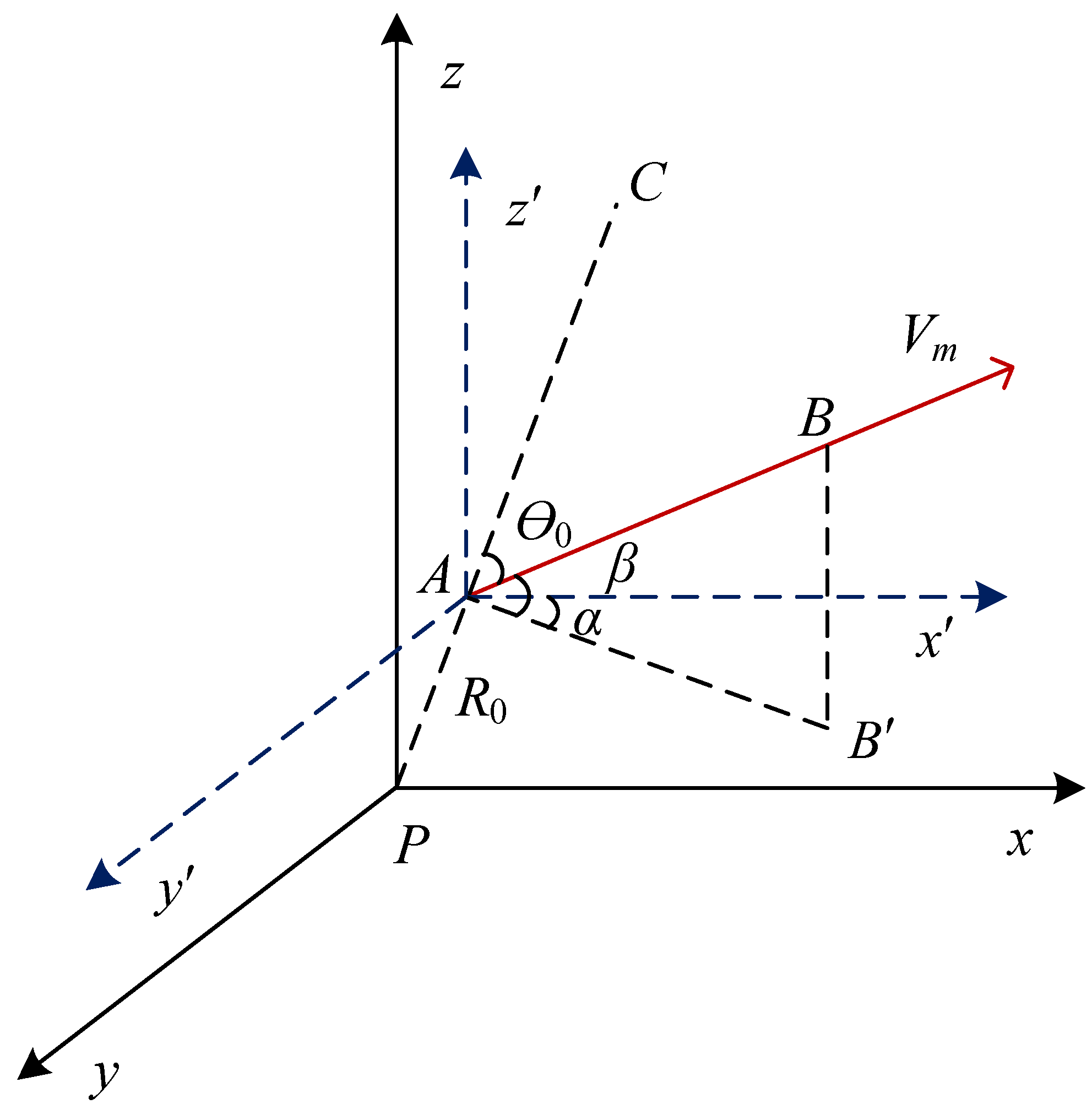
As illustrated in Figure 1, the global coordinate system and the local coordinate system are employed to describe the radar observation and the target motion, respectively. The origin P marks the radar position. A and B denote the start (i.e., ) and end (i.e., ) locations of a target within a CIT period. Generally, when the target’s maneuverability is not too serious, the target’s moving direction and velocity can be approximated as
where represents the initial radial angle between the radar line of sight () and the target moving direction, and is the initial target speed. K represents the rate of change of the radial angle at . A constant K corresponds to circular motion, and when the motion radius increases, K approaches zero, i.e., the case of rectilinear motion. is the kth ()-order acceleration coefficient derived from Taylor expansion.
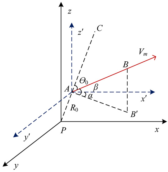
Figure 1.
Geometry of airborne target observation with an HF radar. (P: radar position, : target moving trajectory).
Assuming the global coordinate of A is , then the target coordinate at can be derived as
where and are the azimuth and pitch angle of the target motion, respectively. The corresponding radial distance between target and radar can be expressed as
where is the initial radial range, and is the length of the moving trajectory until
In addition, can also be approximated by Taylor expansion as
where denotes the initial radial speed, and denotes the kth-order derivative of evaluated at . When , and .
In microwave radar data processing, the integration time is usually in the range of tens of milliseconds. Hence, the contribution of for a large k is negligible compared with the first two terms of (10). For most cases, (10) can be accurately described using a second-order relationship, i.e., . However, the case is different for HF radar, which often employs a CIT of several minutes to deal with the sea surface observation. To explore the potential of previous HF radar systems in high-speed target detection, an integration over several minutes is thus required. Considering that HF radar is mainly used for long-range surveillance, where the target usually flies in a regular manner, e.g., roughly rectilinear motion, the model (8) with only three search parameters (i.e., , , ) will be more concise than (10).
2.2. SNR Fluctuation
In the HF band, the RCSs of airplane targets are in the resonance region because the radar wavelength is comparable to the target size [28]. As a result, the signal strength changes significantly with the viewing angle. In addition, the background noise and interference in the HF band are not as stable as those in the microwave band. The above factors lead to the frequent SNR fluctuation of the target signal.
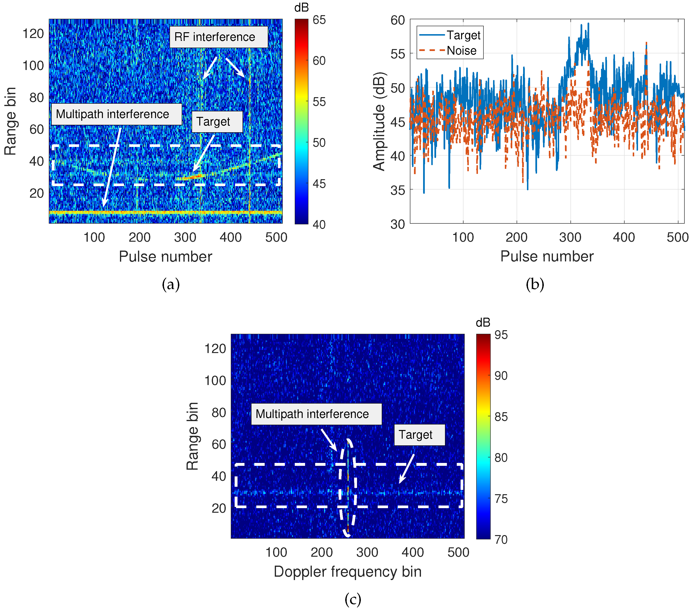
Figure 2 shows real HF radar data including one airplane target. The real data are derived from the same batch as the real data analyzed in Section 5. The radar parameters are available in Table 1. The aircraft’s velocity is 225.3 m/s with a heading of 24.4°, and both its velocity and heading remain essentially constant during the accumulation time. The initial radial range between the target and the radar is 27.7 km. The RM and SNR fluctuation of the target signal are clearly seen in the pulse compression results in Figure 2a. The ground clutter and radio frequency (RF) interference are also evident. Figure 2b compares the variation in target signal strength and the noise floor. It is observed that the signal power changes over a range of about 25 dB and it significantly exceeds the noise floor only in partial pulses. Figure 2c is the corresponding range–Doppler spectrum obtained via the direct fast Fourier transform of Figure 2a in the slow-time domain. In addition to the evident Doppler spreading due to RM, the decline in target SNR is also observed.
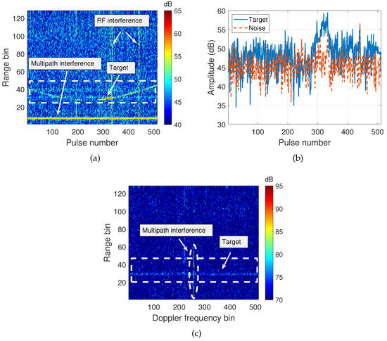
Figure 2.
Real HF radar data. (a) Pulse compression result. (b) Amplitude variation in the target signal (blue) and noise floor (red). (c) Range–Doppler spectrum.

Table 1.
Simulation configuration.
For a moving target without RM, DFM, and amplitude variation, the ideal SNR gain after the coherent integration of (4) is M because the signal power has a gain of and the noise power only increases by a multiple of M. The effect of migration can be mostly mitigated by introducing the motion model (8), but the SNR fluctuation in target signal in Figure 2a still deteriorates the coherent integration. The main reason is that while the signal gain drops due to the fluctuation, the noise gain remains stable.
3. Long-Time Integration via AFS-GRFT Method
By fully considering the difference between HF radar and other microwave radars, an AFS-based GRFT method is proposed to deal with the aforementioned challenges. The basic idea is to alleviate the effect of noise by incorporating an AFS process combined with a GRFT for RM and DFM correction.
3.1. Definition of GRFT
The phase term is modulated by the initial radial range , radial angle , and moving distance of the target. The GRFT of is defined as
where denotes the searching radial range of the target:
is the searching initial radial range, is the searching moving distance, is the searching speed, and is the searching radial angle.
Inserting (11) and (13) into (12), we obtain the GRFT output under different search parameters as
where is the radar resolution. When the search parameters satisfy , GRFT is equal to ideal Fourier transform without range and Doppler migration, and the corresponding integration gain is
In this scenario, both RM and DFM are effectively eliminated, and the search parameters associated with the highest GRFT output correspond to the estimation result. Nonetheless, the real integration gain or the GRFT peak amplitude is affected by the SNR fluctuation issue. As SNR fluctuation increases, the integration gain drops due to the signal power loss in more and more pulses. This effect will be particularly significant for weak target detection, in which case many local maxima (peaks) will appear in the GRFT output results.
The constant false alarm ratio (CFAR) detector with a high false alarm rate is applied to the GRFT output to initially determine the presence or absence of a target
where represents the adaptive threshold determined based on the desired false alarm rate [29]. If the maximum value of exceeds the threshold, the next step will be to estimate the motion parameters. Otherwise, the algorithm terminates, declaring that no target exists. Under the case of in (16), the maximum value is searched by going through all the initial radial range bins, and the corresponding motion parameters are recorded as
where
where , is the maximum number of range bin. Unless otherwise specified, in this article.
Therefore, the candidate target range–time trajectory set can be obtained from the motion parameters estimation. For the ith trajectory, the corresponding motion trajectory can be represented as
At this stage, the CFAR detector (16) with a high false alarm rate is used to ensure a sufficiently high detection probability. The final false alarm rate will be decreased by subsequent AFS processing.
3.2. Amplitude Fluctuation Suppression Based on Non-Coherent Integration
The target’s SNR after GRFT is determined by the total target power and the total noise power, which can be expressed as
where denotes the powers of target and noise at the pulse . In the absence of target amplitude fluctuation, values are comparable for different values of m. However, for HF radar, since the target amplitude fluctuation due to RCS fluctuation is unavoidable, may be even lower than the noise floor at some pulses. As a result, the signal power gain drops but the noise power gain keeps constant; thus, the SNR of GRFT output drops.
The basic idea of AFS is to identify the pulses with very low SNR and remove them, and the remaining pulses are individually processed for target detection. After the AFS operation, since low SNR pulses are eliminated, the target power gain remains basically unchanged, while the noise power gain decreases linearly. As a result, the target SNR can be improved. Considering that the remaining pulses are temporally incontinuous, coherent integration is inapplicable due to the discontinuity of phase information. Non-coherent integration [24] that relies only on the target amplitude information can address this problem.
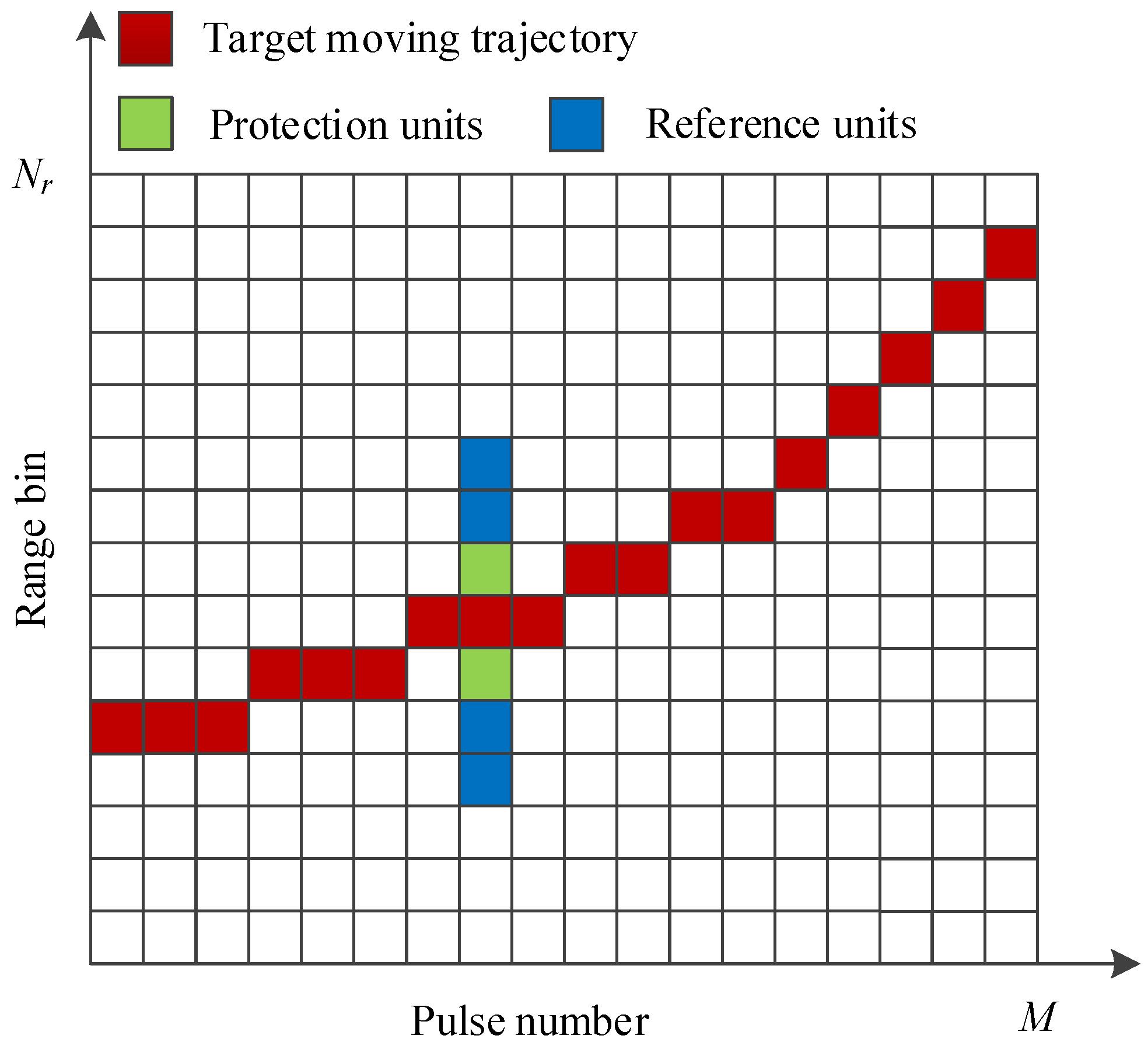
The low SNR pulses are identified through range-domain cell detection, as illustrated in Figure 3. The number of maximum range bins is . The red cells represent the candidate trajectory detected from the GRFT output, with a time resolution of and a range resolution of . To identify the pulses with very low SNR, a range window with a cell length is designed for each pulse. The window is centered at the detection cell, while the adjacent cells (green) are selected as the protection cells and cells (blue) are set as the reference cells. The setting of the protection window length and reference window length should consider the characteristics of the pulse compression signal. Among them, the reference window length setting generally only needs to reflect the average amplitude of the noise; usually, is enough. The length of the protection window is mainly related to the target’s mobility and the range resolution of the radar. In addition, since the first side lobe energy of the target is often strong, the protection window needs to include one range bin above and below the target.
where represents the radial range change during the mth pulse, represents the maximum radial velocity of the target within the change time, and ⌊⌋ denotes the floor function. In this article, the maximum radial velocity of the aircraft is less than 300 m/s. Therefore, is generally taken to be 2.
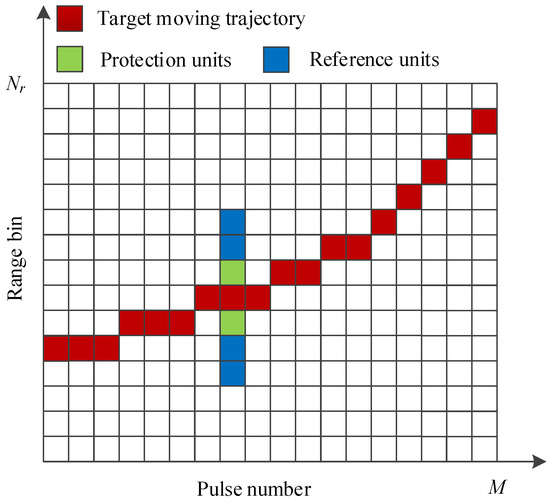
Figure 3.
SNR fluctuation identification through range–time thresholding.
If the signal amplitude of the detection cell is lower than the average amplitude of the reference cells, the corresponding pulse is regarded as low SNR and removed by setting its value as zero.
Furthermore, the amplitude of is accumulated through an non-coherent integration. The result of the ith trajectory can be expressed as
Based on the AFS-GRFT results, a strategy combining peak search and threshold comparison is employed to refine the target detection. If the peak of is much higher than the average level of , the peak can be claimed as a target, which is a binary hypothesis testing problem
where
where denotes the number of candidate target range–time trajectories by (19).
Through AFS and subsequent non-coherent accumulation, the difference in accumulation gain between target and non-target signals will be amplified; thus, AFS-GRFT will output target peaks with higher SNR than that of GRFT. Furthermore, we consider employing an adjustable average accumulation amplitude of all candidate trajectories as the threshold. The threshold is higher than the average amplitude of with a scaling factor ℓ. A larger ℓ leads to a lower false alarm rate as well as a lower detection probability. ℓ needs to be set based on experience. Under the case of , the algorithm terminates and declares that no target exists. Under the case of , the final target trajectory can be estimated by searching for the peak of
3.3. Block Diagram
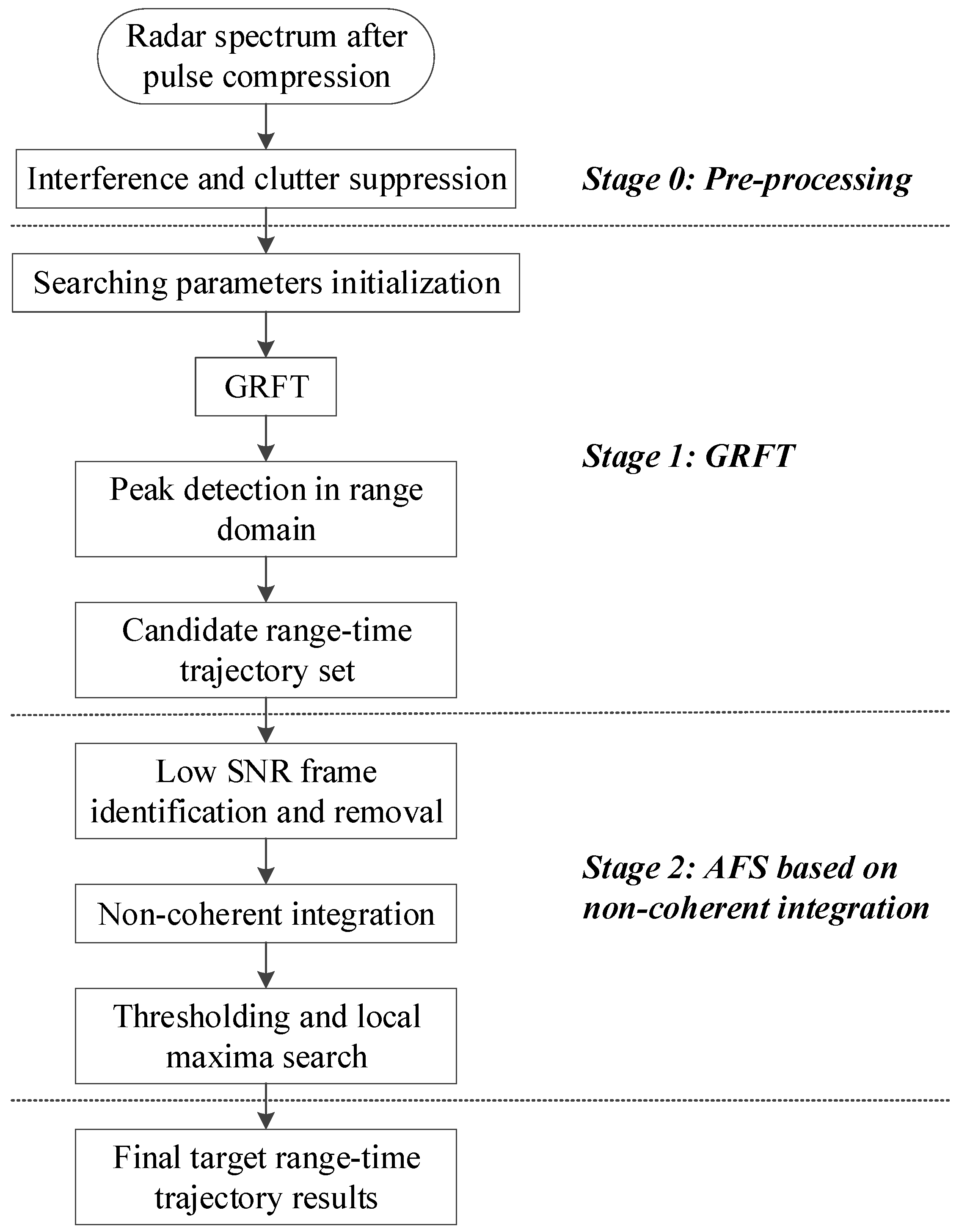
Figure 4 depicts the flowchart of the proposed AFS-GRFT algorithm, which includes two main stages, GRFT and AFS processing based on non-coherent integration. In addition, radar data pre-processing is required in advance. The three stages are summarized as shown below.
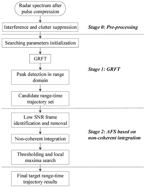
Figure 4.
Flowchart of the proposed AFS-GRFT algorithm.
3.3.1. Stage 0: Pre-Processing
After obtaining the radar echo spectrum through pulse compression, the first stage before applying the proposed target detection method is to remove the interference and clutter, such as radio interference and ground and sea clutter. This can be achieved via spatial or slow-time filtering [30,31]. Ground clutter in high-speed target detection leads to a high false alarm rate, whereas the impact of sea clutter and radio frequency interference is relatively minor. Consequently, this study solely focuses on suppressing ground clutter.
3.3.2. Stage 1: GRFT
Before applying GRFT for RM and DFM correction, it is required to initialize the search parameters, i.e., to design the search scope and interval of each parameter in (13). The search scope and interval directly determine the computation complexity. They should be set according to the radar’s waveform configuration and measurement performance as well as the target’s characteristics [32].
where
3.3.3. Stage 2: AFS Based on Non-Coherent Integration
Since a very low threshold has been employed to obtain the candidate target trajectory set from GRFT outputs, many false alarms will occur. For the weak targets with SNR fluctuation, the false alarm rate is particularly high because the contribution of noise is much more than that of signal. Hence, the first key step is to identify the pulses with very low SNR and remove them via (22). The second step is to take non-coherent integration over the remaining pulses via (23).
Through the above AFS processing, the spectral amplitude difference between target and non-target will be enlarged. Therefore, the target can be further detected according to binary hypothesis testing (24), and the corresponding target range–time trajectory result can be obtained from (26).
For the multi-target scenario, to avoid the effect of strong target on weak target, the target detection is carried out by a one-by-one strategy instead of at one time. After a strong target is detected based on the proposed AFS-GRFT method, it is removed from the range–time spectrum by using the CLEAN technique [33,34] before detecting the next target. The case study of a two-target scenario will be presented in Section 5.2.
4. Numerical Simulation
In this article, civil aircraft targets are investigated; thus, the algorithm search configuration is set according to the characteristics of these targets to optimize the computation complexity. Generally, the flying speed of civil aircraft targets is within the range of 200–300 m/s, and the speed variation during a CIT period of HF radar is less than 10%. For simplicity, the search parameters and are excluded from the simulation, and the investigation focuses on the effect of SNR fluctuation. The simulation configuration is listed in Table 1. It should be noted that and can be taken into account according to the practical demand just at the cost of computation complexity. In this scenario, the computational complexity of GRFT is , while that of AFS-GRFT is . Among them, , , and represent the number of search parameters in GRFT. The additional computational complexity introduced by AFS operation can be negligible compared with that of GRFT.
4.1. Metrics Definition
To study the performance of the proposed method under different SNR fluctuation conditions, the rate of SNR fluctuation is defined in advance. Given the CIT period of M pulses, is defined by the ratio of the number of low SNR pulses to M. In the simulation, the low SNR pulses are randomly selected and set to zero power for simplicity. In experimental data, the pulses with a power lower than the average noise power are regarded as the low SNR pulses.
The target SNR is defined as the ratio of the total signal power to the total noise power over all pulses. It is evident that a higher means a lower SNR. For clarity, we use to denote the target SNR associated with a specific .
where
where and denote the target and noise power, respectively. is the number of range cells taken for noise power calculation. Different implies that a different number of low SNR pulses are included in .
Finally, the root mean square error (RMSE) defined as follows is used to express the search accuracy of high-speed targets.
where and represent the estimated and real range–time trajectories of the target, respectively.
A successful detection is defined by a search error less than . The detection probability can be represented by the ratio of the number of successful detections to that of the total trials.
4.2. Algorithm Flow Validation
The purpose of this subsection is to validate the flow of the proposed algorithm and compare its performance with traditional GRFT. According to the aforementioned description, the proposed AFS-GRFT is superior to that of GRFT when the SNR is low and SNR fluctuation is serious. Theoretically, if no SNR fluctuation occurs, the two methods should be equivalent in detection performance. To clarify the difference between the two methods, two SNR fluctuation conditions are considered:
4.2.1. dB
Figure 5a shows the pure target signal after pulse compression, and Figure 5b depicts the signal plus real radar spectrum which includes only the background noise and RF interference. Initially, the target SNR is set to be −15 dB for each pulse. Then, the SNR fluctuation rate is set to 0.83, and the final SNR defined by (36) can be calculated as dB. The change in signal amplitude and noise level is compared in Figure 5c, where 83% (425 of 512) of pulses are being submerged by noise.
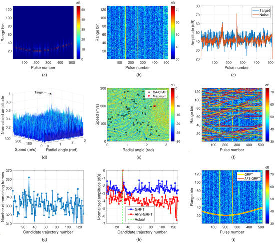
Figure 5.
Simulation results of target range–time trajectory detection at dB. (a) Pure target signal without noise. (b) Signal plus real background noise and interference. (c) Amplitude change in target signal and noise. (d) AFS-GRFT result of (b) at km. (e) Comparison of CFAR and peak detection results of (d). (f) Candidate range–time trajectory set. (g) Number of remaining pulses after low SNR pulses removal. (h) Amplitude comparison of GRFT and AFS-GRFT outputs. (i) Final range–time trajectory detection results.
Figure 5d presents the GRFT result of Figure 5b at km, and the peak associated with the target is clear. Figure 5e compares the GRFT detection results using the cell average (CA)-CFAR and peak detectors. It is observed that there are many peaks around the maxima, which are actually the blind speed sidelobes (BSSL) of the target signal. This issue will trouble the target detection, particularly in multi-target scenarios. Hence, peak detection rather than CFAR detector is preferred at this stage, which will be further illustrated in Section 5.2. The complete candidate range–time trajectory set is plotted in Figure 5f.
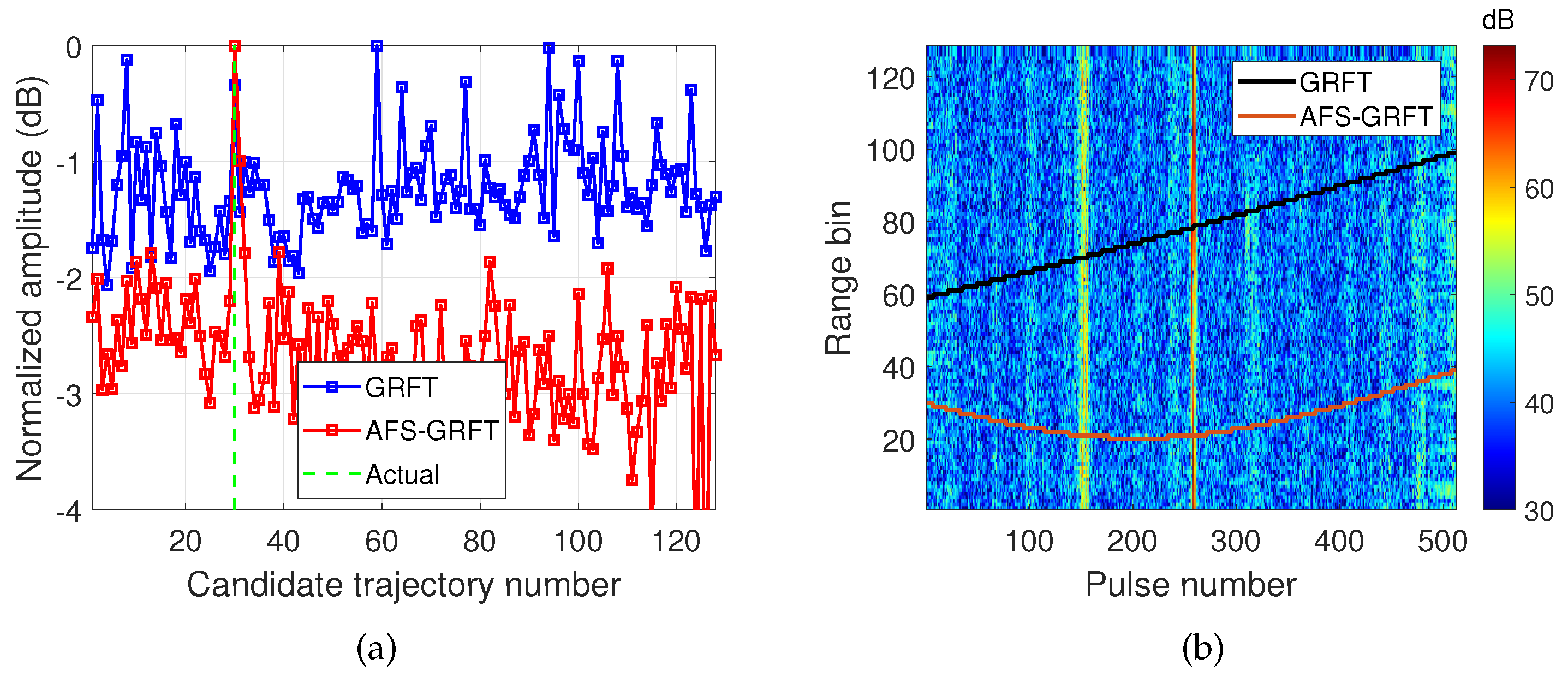
For each candidate trajectory, low SNR identification and removal are conducted, and the number of remaining pulses associated with different candidate trajectories is given in Figure 5g. The trajectory corresponding to the real target has slightly more remaining pulses than the others. For the proposed AFS-GRFT method, the remaining pulses are further processed through non-coherent integration. Figure 5h shows the normalized (w.r.t. maxima) amplitude results of GRFT and AFS-GRFT, where the x-axis represents the sequence number of the candidate trajectory, which is i in (19). It is found that both GRFT and AFS-GRFT output an evident peak associated with the right target trajectory, but the peak generated by AFS-GRFT has a higher SNR than that of GRFT. Figure 5i depicts the corresponding detection results, and both methods obtain the right detection.
4.2.2. dB
Further comparison is conducted by increasing from 0.83 to 0.88, and the resulting SNR decreases by about 1.55 dB. Figure 6 shows similar results to Figure 5h,i. It can be inferred by comparing Figure 6a and Figure 5h that the peak SNRs of both GRFT and AFS-GRFT fall as falls. However, AFS-GRFT still has an SNR gain of several decibels greater than that of GRFT. Hence, in this case, AFS-GRFT can correctly detect the target trajectory but GRFT cannot (see Figure 6b).

Figure 6.
Similar results as Figure 5h,i for dB.
4.3. Analysis of Detection Probability and Search Accuracy
Monte Carlo simulations are conducted to further assess the statistical performance of the proposed algorithm at different SNR levels and fluctuation rates. For each test, 500 Monte Carlo trials are carried out.
4.3.1. Detection Probability
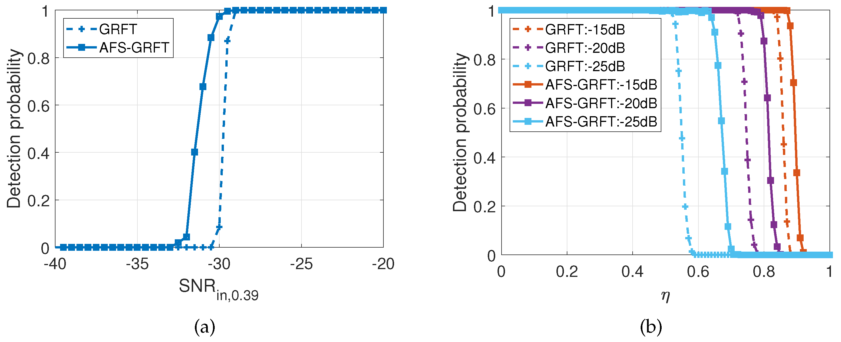
Figure 7 shows the simulation results of detection probability. In Figure 7a, a constant is chosen and is adjusted by changing the signal power, i.e., . It is seen that the performance of both algorithms drops as SNR decreases, but the minimum detectable SNR level of AFS-GRFT is about 2 dB lower than that of GRFT. In Figure 7b, three different values (−15 dB, −20 dB, −25 dB) are selected, and is adjusted by changing . As increases, falls. It is noticed that the maximum detectable of AFS-GRFT is higher than that of GRFT, and the performance difference between the two methods increases as the target SNR drops. In other words, AFS-GRFT outperforms GRFT more significantly in lower SNR and more serious SNR fluctuation conditions.
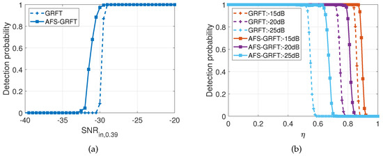
Figure 7.
Simulation results of detection probability versus (a) SNR () and (b) SNR fluctuation rate .
4.3.2. Search Accuracy
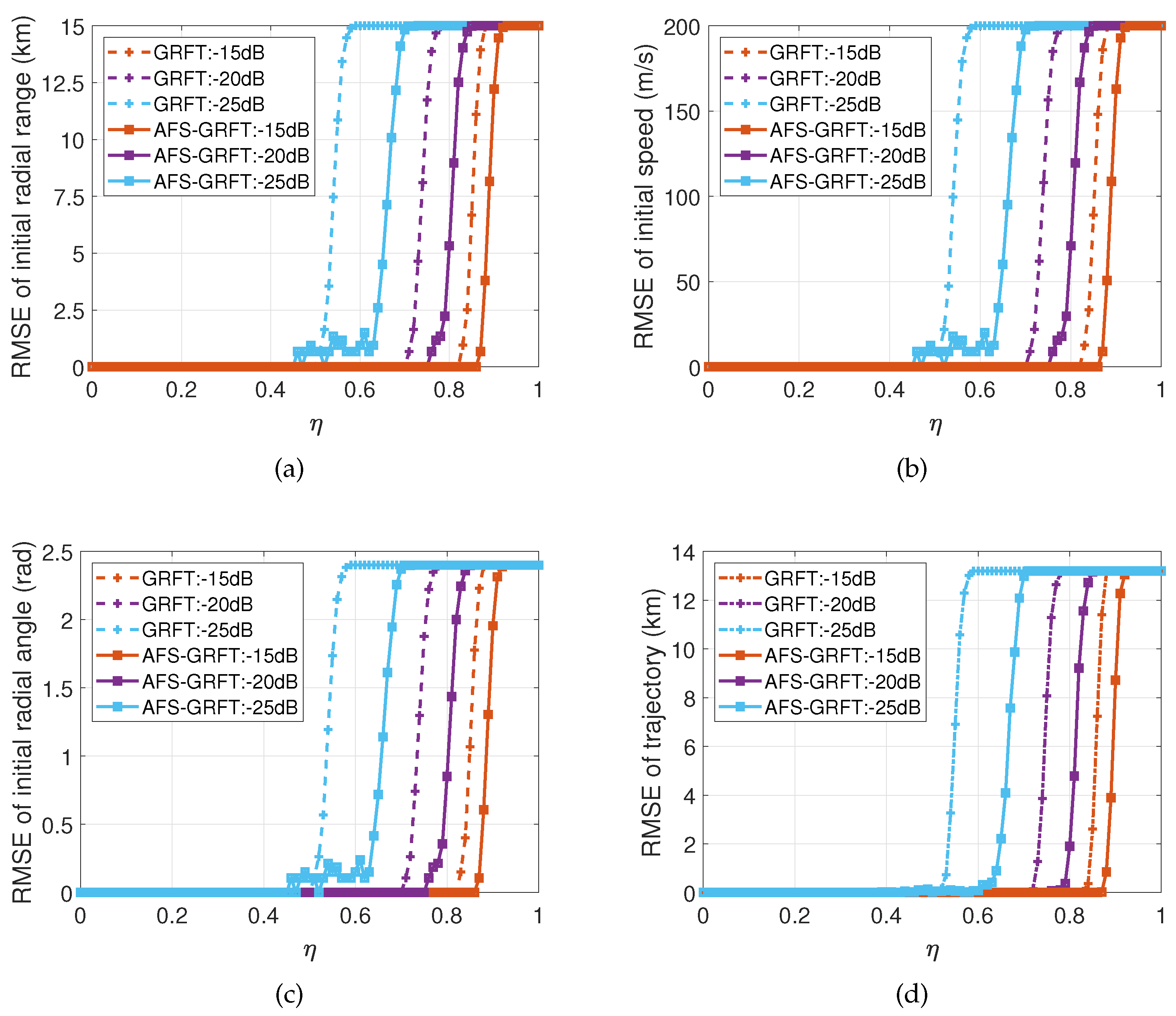
In addition to the detection probability, the algorithm performance is evaluated regarding the parameters’ search accuracy. Figure 8 demonstrates the search error results of , , , and , respectively. The search error of all parameters increases as the SNR fluctuation rate increases. Given the same , AFS-GRFT always surpasses GRFT. It is noticed that for the case of AFS-GRFT at dB, the simulated RMSE- curves are not as smooth as the others. This is mainly due to the limited number of Monte Carlo trials.
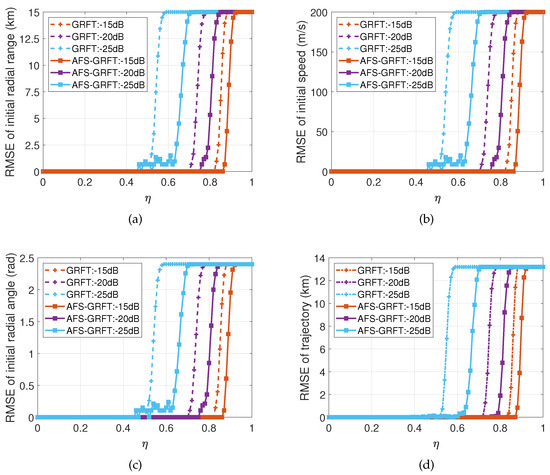
Figure 8.
Simulation results of target parameters search error. (a) . (b) . (c) . (d) .
Note that the difference between simulation and reality always exists because the background noise and interference as well as the SNR fluctuation model of signal are much more complicated in reality than in simulation. More investigation using the experimental data will be given in Section 5.
5. Experimental Results
The experimental data used to verify the proposed algorithm were collected by a compact HF radar system [7] in April 2022. The radar waveform configuration refers to Table 1. In addition, the average transmit power is 100 W, and the transmitting antenna employs a monopole while receiving with a crossed-loop antenna, which are both with low gain and compact size. Hence, the detection performance is limited compared with the large phased-array HF radar systems with very high transmitting power. Nevertheless, the application of the proposed algorithm to the two different kinds of systems is the same; thus, it does not influence the algorithm validation.
The civil aircraft targets are investigated, and the information provided by the Automatic Dependent Surveillance-Broadcast (ADS-B) receiver was selected as the ground truth, including the location, speed, heading, its identification, known as the International Civil Aviation Organization (ICAO) address, etc. Before the comparison, the ADS-B data are temporally aligned with the radar data through interpolation.
5.1. Single Target Detection Results
Table 2 lists the detection results of six targets. AFS-GRFT is compared with GRFT in terms of three search parameters, , , and , and the RMSE of the range–time trajectory . It is found that AFS-GRFT produces more accurate detection results than GRFT for targets #1–3 and 5–6, and the two methods show the same accuracy only for target #4. In addition, the difference in SNR between targets #1 and #5–6 is large. Therefore, the detailed processing results of target #1 and 4–6 are selected for illustration.
Table 2.
Experimental comparison between GRFT and AFS-GRFT for six datasets.
5.1.1. Data #1
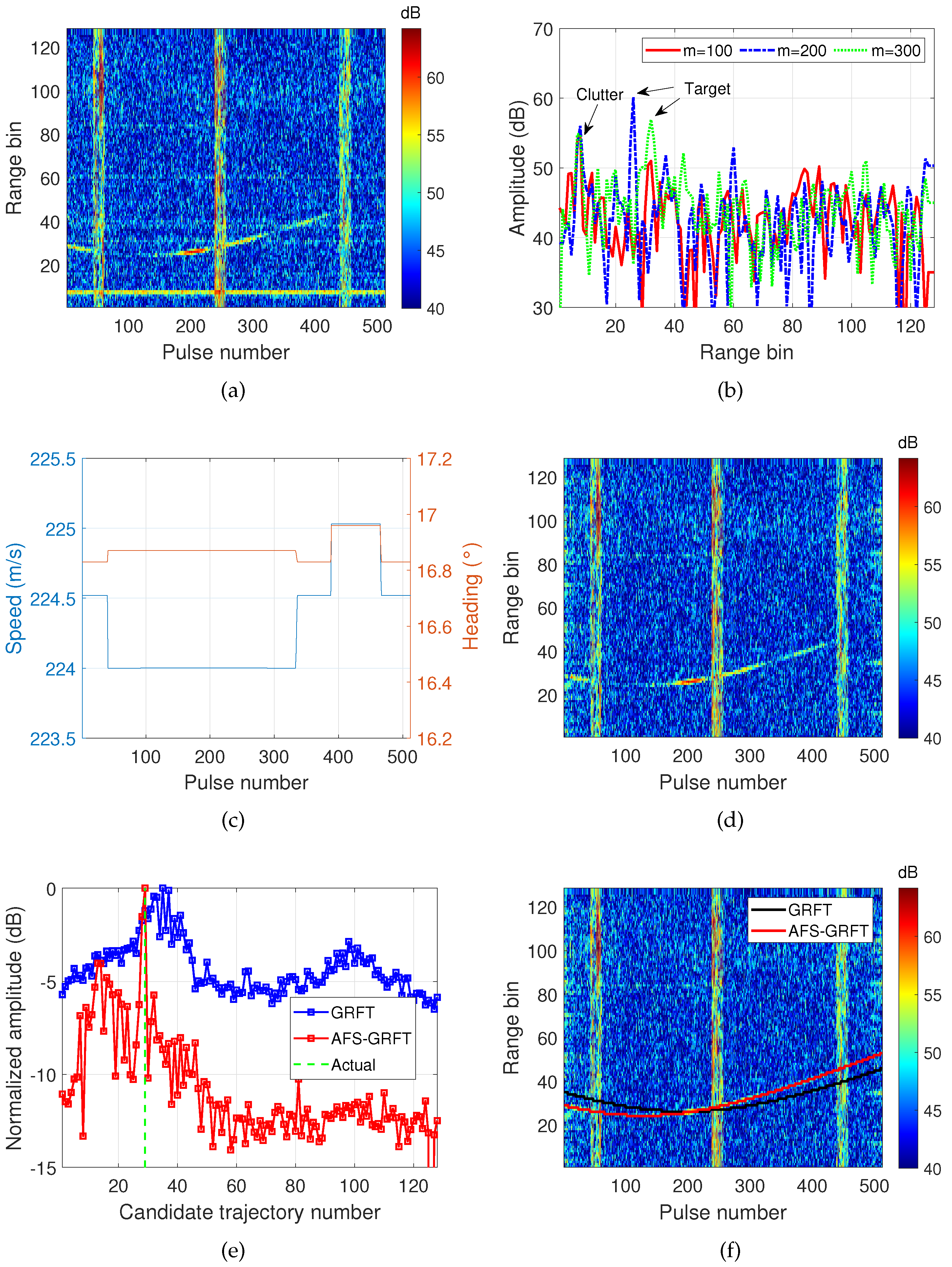
Figure 9 shows the processing results of target #1. It is seen in Figure 9a,b that both the amplitude and range of the target signal change significantly across pulses, which is submerged by the noise floor in many pulses. During the CIT period of 512 pulses, the variation in the target’s speed and heading as illustrated in Figure 9c are 1 m/s and 0.13°, respectively, which can be regarded as a uniform rectilinear motion. Hence, the search motion is simplified with three parameters, , , and .
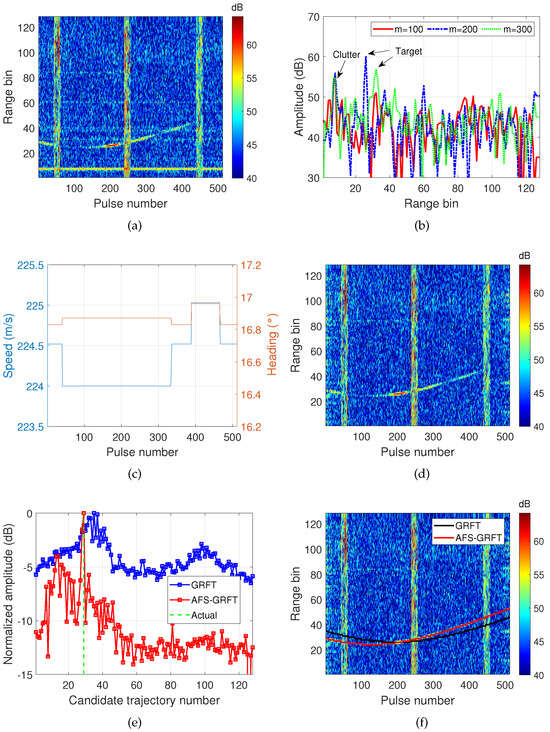
Figure 9.
Experimental results of range–time trajectory detection (data #1). (a) Original pulse compression result. (b) Range profiles of the 100th, 200th, and 300th pulses. (c) True speed and heading of the airplane target reported by ADS-B. (d) Ground clutter-suppressed result of (a). (e) Re-integrated result with normalized amplitude. (f) Final range–time trajectory detection result.
Figure 9d presents the radar range–time spectrum after removing the ground clutter through high-pass filtering over the slow-time domain. It is worth noting that GRFT mainly takes into account the temporal-varied range information; thus, the impulse RF interference that occurs at specific times does not trouble the detection as much as the ground clutter. Figure 9e,f compare the detection results between GRFT and AFS-GRFT. The peak location of AFS-GRFT output agrees well with the real target site; however, a bias appears in GRFT’s result. Moreover, the peak of AFS-GRFT is much narrower than that of GRFT, which is beneficial for improving the detection accuracy and decreasing the false alarm rate. The final trajectory detection RMSEs of GRFT and AFS-GRFT are 1.79 km and 0.49 km, respectively.
5.1.2. Data #4, #5, and #6
The similar results of targets #4–6 are demonstrated in Figure 10. Overall, a higher generates a lower RMSE of . The proposed AFS-GRFT method is superior to GRFT except for the case of target #4, where the two methods show the same detection performance. For targets #5–6, since their SNRs are lower than the minimum detectable threshold, GRFT fails to detect the range–time trajectory. For target #5, the estimation of AFS-GRFT is slightly larger than that of the other targets. The reason is that during the first few pulses, target #5 was basically moving in the tangential direction perpendicular to the radar line of sight, where the target’s range change is small and the radial speed approximates zero. Due to the radar resolution limitation, it is thus hard to search for an accurate .

Figure 10.
Similar results as Figure 9a,e,f. (a–c) Data #4. (d–f) Data #5. (g–i) Data #6.
5.2. Multi-Target Detection Results
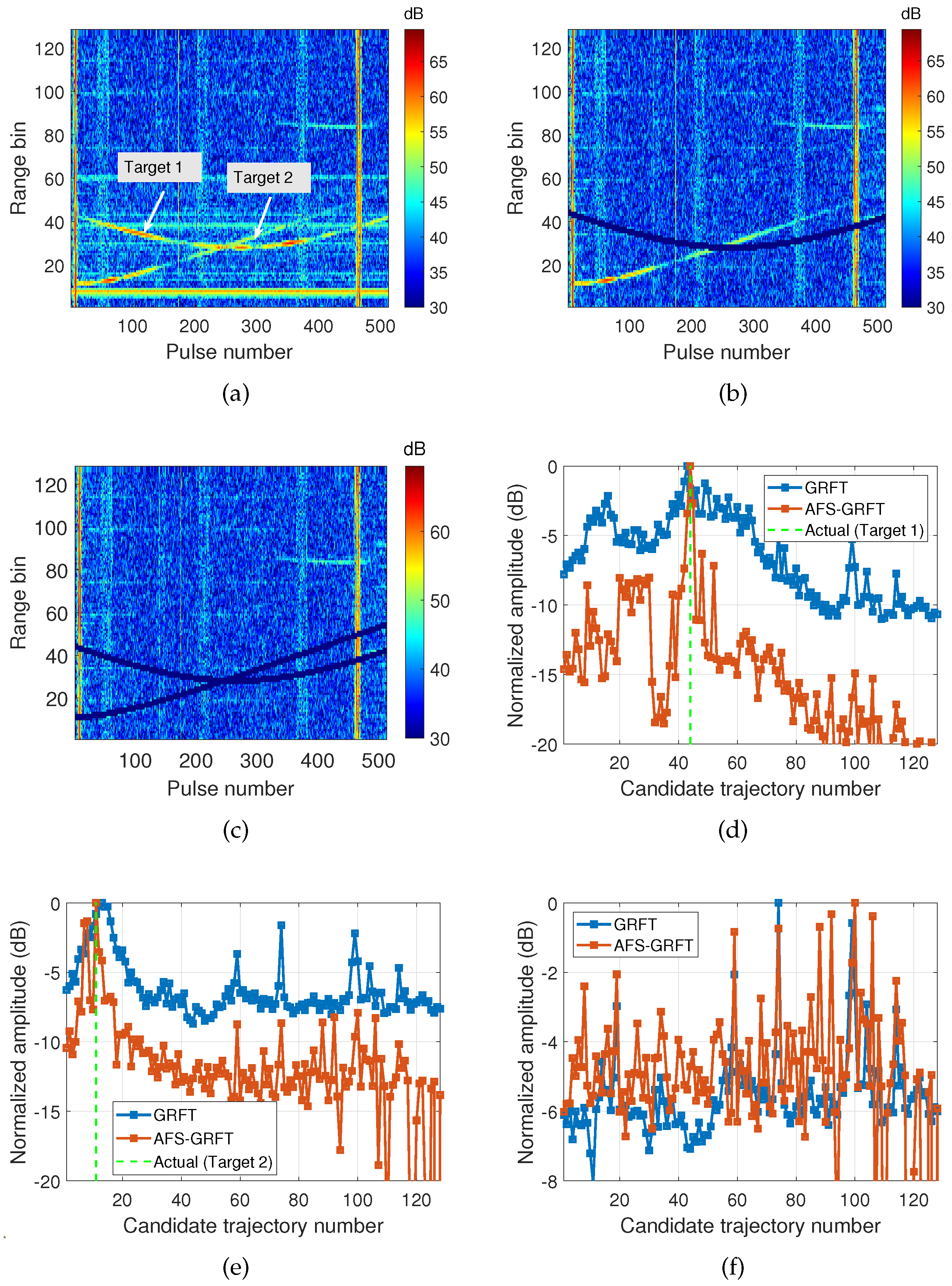
In multi-target scenarios, the fluctuation in SNR often results in significant SNR differences among targets. The sidelobe effects of strong targets in GRFT may hinder the detection of weak targets, leading to false alarms and missed detections. Therefore, to cover the case of simultaneously detecting strong and weak targets, the detection flow of a multi-target scenario is divided into multiple single-target detection steps, as briefly introduced in Section 3.3. At each step, the strongest target is first detected and then it is removed from the radar spectrum through the CLEAN algorithm [33,34] before the next detection.
Figure 11 illustrates the detection result of a two-target case. For fairness of comparison, both GRFT and AFS-GRFT employ the same CLEAN processing. In Figure 11a, the range–time trajectories associated with two targets intersect and both suffer from serious SNR fluctuation. Figure 11d shows the detection results of step 1, where both GRFT and AFS-GRFT successfully detect target #1 (corresponding to km). In addition, it is also observed that there are two other local peaks appearing at about km and 50 km, respectively. If we directly detect multiple targets at one stage by searching all of the local peaks on GRFT or AFS-GRFT spectra, there will be many false alarms, and the weak targets will be seriously contaminated by the strong targets. Figure 11b shows the range–time spectrum after removing target #1 using the CLEAN algorithm, and the following detection result is illustrated in Figure 11e. Subsequently, target #2 is removed from the range–time spectrum (see Figure 11c), and the third detection is made, as depicted in Figure 11f. If no more candidate target is found, the multi-target detection is terminated. The detection errors are compared in Table 3. Since both targets have a sufficiently high SNR, GRFT and AFS-GRFT produce comparable detection accuracy. For target #2, the detection error of AFS-GRFT is slightly lower than that of GRFT. It is noticed from Figure 11f that GRFT produces several local peaks, even when no more targets exist, but AFS-GRFT only generates a noise without evident peaks. Hence, it can be inferred that GRFT would cause more false alarms than AFS-GRFT. Due to the data number limitation, the statistical analysis of the false alarm rate is not available here.
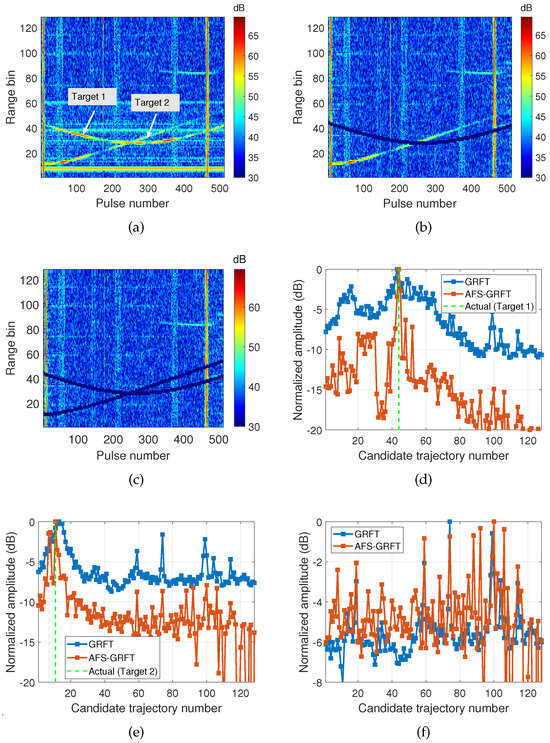
Figure 11.
Experimental case of multiple targets. (a) Original pulse compression result. (b,c) Pulse compression results after removing target #1 and #2 by CLEAN algorithm, respectively. (d–f) GRFT and AFS-GRFT outputs of (a–c), respectively.
Table 3.
Target detection errors of Figure 11.
5.3. Discussion
The experimental results demonstrate that the proposed AFS-GRFT algorithm can obtain more accurate motion estimation than that of GRFT in dealing with high-speed target detection, and the superiority is particularly outstanding under low SNR and serious SNR fluctuation conditions. However, there are still some factors that would affect the application of the proposed method, which ought to be further discussed.
5.3.1. Computation Complexity
This article mainly focuses on addressing the effect of SNR fluctuation on long-time integration, and the investigated targets’ motion is relatively simple. If a more complex maneuver occurs when the aircraft is in the phase of takeoff, landing, turning, etc., the problem will be more complex. Theoretically, AFS-GRFT can adapt to arbitrary motion models as GRFT does by introducing more searching parameters at the expense of exponentially increasing computation complexity. Compared with microwave radar, the detection time allowed by HF radar is much longer. Moreover, the computation efficiency of the GRFT algorithm can also be improved through many tricks, such as frequency bin RFT (FBRFT) [35], sub-band RFT (SBRFT) [35], etc.
5.3.2. Complex Multi-Target Scenario
The preliminary result of multi-target detection demonstrates the effectiveness of the proposed method. It should be noted that when the multi-target scenario is more complex, e.g., including (i) more targets, (ii) both strong and weak targets, and (iii) range–time close trajectories, the algorithm performance may be challenging, and more validation is required.
5.3.3. Complex Interference and Clutter
In this article, the experimental data contain only the ground clutter and impulse interference, which occurs at specific times (refer to Figure 9a, Figure 10a, Figure 10g and Figure 11a). The case may be more complex for different radar frequencies, sites, and electromagnetic environments. For example, if the radar spectrum includes sea clutter, ionospheric clutter, successive radio interference, etc., more work should be concentrated on suppressing the clutters and interference.
6. Conclusions
In this article, long-time integration involving high-speed target detection with HF radar is studied. To improve the detection ability of HF radar (particularly a compact HF radar), which is commonly limited by low SNR and serious SNR fluctuation conditions, an AFS-GRFT method employing a combined coherent and non-coherent detector is proposed. GRFT-based coherent integration is used to obtain the candidate trajectory set. At this stage, a high detection probability at the expense of a high false alarm rate is designed. Subsequently, low SNR pulses identification and removal followed by a non-coherent integration is carried out to reduce the false alarm rate and refine the motion detection accuracy. Numerical simulation and field experiment results demonstrate that the proposed AFS-GRFT method outperforms the existing coherent integration algorithm GRFT regarding detection probability and motion estimation accuracy. Moreover, AFS-GRFT exhibits robust performance in multi-target detection scenarios. The ongoing work will include the further investigation of the false alarm statistics based on the analysis of more and longer experimental data and the further validation of the proposed method under different clutter and interference backgrounds. The application of the method to different radar systems such as the long-range sky-wave radar will also be taken into account in the future.
Author Contributions
Methodology, G.L., Y.T. and B.W.; validation, Y.T. and B.W.; writing—original draft, G.L.; writing—review and editing, Y.T., B.W. and C.L. All authors have read and agreed to the published version of the manuscript.
Funding
This work was supported in part by the National Key R&D Program of China under Grant 2022YFC2806300; in part by the National Natural Science Foundation of China under Grant 62071337; in part by the Natural Science Foundation of Hubei Province under Grant 2022CFB055; and in part by the Guangdong Basic and Applied Basic Research Foundation under Grant 2024A1515011961.
Data Availability Statement
The raw data supporting the conclusions of this article will be made available by the authors on request.
Acknowledgments
We thank the editor and the anonymous reviewers for their constructive suggestions.
Conflicts of Interest
The authors declare no conflicts of interest.
References
- Khan, R.; Gamberg, B.; Power, D.; Walsh, J.; Dawe, B.; Pearson, W.; Millan, D. Target detection and tracking with a high frequency ground wave radar. IEEE J. Ocean. Eng. 1994, 19, 540–548. [Google Scholar] [CrossRef]
- Khan, R.H.; Power, D. Aircraft detection and tracking with high frequency radar. In Proceedings of the International Radar Conference, Alexandria, VA, USA, 8–11 May 1995; pp. 44–48. [Google Scholar]
- Earl, G.; Ward, B. The frequency management system of the Jindalee over-the-horizon backscatter HF radar. Radio Sci. 1987, 22, 275–291. [Google Scholar] [CrossRef]
- Francis, D.B.; Cervera, M.A.; Frazer, G.J. Performance prediction for design of a network of skywave over-the-horizon radars. IEEE Aerosp. Electron. Syst. Mag. 2017, 32, 18–28. [Google Scholar] [CrossRef]
- Anderson, S. Counter-OTHR 101: Low observability at HF. In Proceedings of the International Conference on Radar Systems (RADAR 2022), Edinburgh, UK, 24–27 October 2022; pp. 405–410. [Google Scholar]
- Tao, R.; Zhang, N.; Wang, Y. Analysing and compensating the effects of range and Doppler frequency migrations in linear frequency modulation pulse compression radar. IET Radar Sonar Navig. 2011, 5, 12–22. [Google Scholar]
- Lu, B.; Wen, B.; Tian, Y.; Wang, R. A vessel detection method using compact-array HF radar. IEEE Geosci. Remote Sens. Lett. 2017, 14, 2017–2021. [Google Scholar] [CrossRef]
- Li, G.; Xia, X.-G.; Peng, Y.-N. Doppler keystone transform: An approach suitable for parallel implementation of SAR moving target imaging. IEEE Geosci. Remote Sens. Lett. 2008, 5, 573–577. [Google Scholar] [CrossRef]
- Perry, R.; Dipietro, R.; Fante, R. SAR imaging of moving targets. IEEE Trans. Aerosp. Electron. Syst. 1999, 35, 188–200. [Google Scholar] [CrossRef]
- Zhu, D.; Li, Y.; Zhu, Z. A keystone transform without interpolation for SAR ground moving-target imaging. IEEE Geosci. Remote Sens. Lett. 2007, 4, 18–22. [Google Scholar] [CrossRef]
- Xu, J.; Yu, J.; Peng, Y.-N.; Xia, X.-G. Radon-Fourier transform for radar target detection, I: Generalized Doppler filter bank. IEEE Trans. Aerosp. Electron. Syst. 2011, 47, 1186–1202. [Google Scholar] [CrossRef]
- Rao, X.; Tao, H.; Su, J.; Guo, X.; Zhang, J. Axis rotation MTD algorithm for weak target detection. Digit. Signal Process. 2014, 26, 81–86. [Google Scholar] [CrossRef]
- Kirkland, D. Imaging moving targets using the second-order keystone transform. IET Radar Sonar Navig. 2011, 5, 902–910. [Google Scholar] [CrossRef]
- Sun, G.; Xing, M.-D.; Wang, Y.; Zhou, F.; Wu, Y.; Bao, Z. Improved ambiguity estimation using a modified fractional Radon transform. IET Radar Sonar Navig. 2011, 5, 489–495. [Google Scholar] [CrossRef]
- Chen, X.; Guan, J.; Liu, N.; He, Y. Maneuvering target detection via Radon-fractional Fourier transform-based long-time coherent integration. IEEE Trans. Signal Process. 2014, 62, 939–953. [Google Scholar] [CrossRef]
- Chen, X.; Guan, J.; Liu, N.; Zhou, W.; He, Y. Detection of a low observable sea-surface target with micromotion via the Radon-linear canonical transform. IEEE Geosci. Remote Sens. Lett. 2013, 11, 1225–1229. [Google Scholar] [CrossRef]
- Li, X.; Cui, G.; Yi, W.; Kong, L. Coherent integration for maneuvering target detection based on Radon-Lv’s distribution. IEEE Signal Process. Lett. 2015, 22, 1467–1471. [Google Scholar] [CrossRef]
- Chen, X.; Huang, Y.; Liu, N.; Guan, J.; He, Y. Radon-fractional ambiguity function-based detection method of low-observable maneuvering target. IEEE Trans. Aerosp. Electron. Syst. 2015, 51, 815–833. [Google Scholar] [CrossRef]
- Xu, J.; Xia, X.-G.; Peng, S.-B.; Yu, J.; Peng, Y.-N.; Qian, L.-C. Radar maneuvering target motion estimation based on generalized Radon-Fourier transform. IEEE Trans. Signal Process. 2012, 60, 6190–6201. [Google Scholar]
- Ding, Z.; Liu, S.; Li, Y.; You, P.; Zhou, X. Parametric translational compensation for isar imaging based on cascaded subaperture integration with application to asteroid imaging. IEEE Trans. Geosci. Remote Sens. 2022, 60, 1–17. [Google Scholar] [CrossRef]
- Li, X.; Cui, G.; Yi, W.; Kong, L. A fast maneuvering target motion parameters estimation algorithm based on ACCF. IEEE Signal Process. Lett. 2014, 22, 270–274. [Google Scholar] [CrossRef]
- Cui, G.; DeMaio, A.; Piezzo, M. Performance prediction of the incoherent radar detector for correlated generalized Swerling-chi fluctuating targets. IEEE Trans. Aerosp. Electron. Syst. 2013, 49, 356–368. [Google Scholar] [CrossRef]
- Zhou, X.; Qian, L.; Ding, Z.; Xu, J.; Liu, W.; You, P.; Long, T. Radar detection of moderately fluctuating target based on optimal hybrid integration detector. IEEE Trans. Aerosp. Electron. Syst. 2018, 55, 2408–2425. [Google Scholar] [CrossRef]
- Zhang, Z.; Liu, N.; Hou, Y.; Zhang, S.; Zhang, L. A coherent integration segment searching based GRT-GRFT hybrid integration method for arbitrary fluctuating target. Remote Sens. 2022, 14, 2695. [Google Scholar] [CrossRef]
- Shen, Y.; Zhang, N.; Liu, Y. New waveform with both high range resolution and long coherent integration time in a HF radar. In Proceedings of the International Radar Conference, Beijing, China, 8–10 October 1996; pp. 285–288. [Google Scholar]
- Shen, Y.; Liu, Y.; Wu, A. Coherent phase-coded pulse train with Doppler cascade-processing for detection of aircraft target in a HF radar. J. Syst. Eng. Electron. 1999, 10, 50–56. [Google Scholar]
- Dzvonkovskaya, A.; Rohling, H. Fast-moving target observation using high-frequency surface wave radar. In Proceedings of the 2014 International Radar Conference, Lille, France, 13–17 October 2014; pp. 1–4. [Google Scholar]
- Trueman, C.W.; Kubina, S.J.; Mishra, S.R.; Larose, C. Radar cross-section of a generic aircraft at HF frequencies. Can. J. Electr. Comput. Eng. 1993, 18, 59–64. [Google Scholar] [CrossRef]
- Chen, X.; Yu, X.; Huang, Y.; Guan, J. Adaptive clutter suppression and detection algorithm for radar maneuvering target with high-order motions via sparse fractional ambiguity function. IEEE J. Sel. Top. Appl. Earth Obs. Remote Sens. 2020, 13, 1515–1526. [Google Scholar] [CrossRef]
- Gurgel, K.-W.; Barbin, Y.; Schlick, T. Radio frequency interference suppression techniques in FMCW modulated HF radars. In Proceedings of the OCEANS 2007-Europe, Aberdeen, UK, 18–21 June 2007; pp. 1–4. [Google Scholar]
- Zhou, H.; Wen, B.; Wu, S. Dense radio frequency interference suppression in HF radars. IEEE Signal Process. Lett. 2005, 12, 361–364. [Google Scholar] [CrossRef]
- Li, X.; Sun, Z.; Yeo, T.S.; Zhang, T.; Yi, W.; Cui, G.; Kong, L. STGRFT for detection of maneuvering weak target with multiple motion models. IEEE Trans. Signal Process. 2019, 67, 1902–1917. [Google Scholar] [CrossRef]
- Tsao, J.; Steinberg, B.D. Reduction of sidelobe and speckle artifacts in microwave imaging: The CLEAN technique. IEEE Trans. Antennas Propag. 1988, 36, 543–556. [Google Scholar] [CrossRef]
- Misiurewicz, J.; Kulpa, K.S.; Czekala, Z.; Filipek, T.A. Radar detection of helicopters with application of CLEAN method. IEEE Trans. Aerosp. Electron. Syst. 2012, 48, 3525–3537. [Google Scholar] [CrossRef]
- Yu, J.; Xu, J.; Peng, Y.-N.; Xia, X.-G. Radon-Fourier transform for radar target detection (III): Optimality and fast implementations. IEEE Trans. Aerosp. Electron. Syst. 2012, 48, 991–1004. [Google Scholar] [CrossRef]


Disclaimer/Publisher’s Note: The statements, opinions and data contained in all publications are solely those of the individual author(s) and contributor(s) and not of MDPI and/or the editor(s). MDPI and/or the editor(s) disclaim responsibility for any injury to people or property resulting from any ideas, methods, instructions or products referred to in the content. |
© 2024 by the authors. Licensee MDPI, Basel, Switzerland. This article is an open access article distributed under the terms and conditions of the Creative Commons Attribution (CC BY) license (https://creativecommons.org/licenses/by/4.0/).