Forest 3D Radar Reflectivity Reconstruction at X-Band Using a Lidar Derived Polarimetric Coherence Tomography Basis

Abstract

Tomographic Synthetic Aperture Radar (SAR) allows the reconstruction of the 3D radar reflectivity of forests from a large(r) number of multi-angular acquisitions. However, in most practical implementations it suffers from limited vertical resolution and/or reconstruction artefacts as the result of non-ideal acquisition setups. Polarisation Coherence Tomography (PCT) offers an alternative to traditional tomographic techniques that allow the reconstruction of the low-frequency 3D radar reflectivity components from a small(er) number of multi-angular SAR acquisitions. PCT formulates the tomographic reconstruction problem as a series expansion on a given function basis. The expansion coefficients are estimated from interferometric coherence measurements between acquisitions. In its original form, PCT uses the Legendre polynomial basis for the reconstruction of the 3D radar reflectivity. This paper investigates the use of new basis functions for the reconstruction of X-band 3D radar reflectivity of forests derived from available lidar waveforms. This approach enables an improved 3D radar reflectivity reconstruction with enhanced vertical resolution, tailored to individual forest conditions. It also allows the translation from sparse lidar waveform vertical reflectivity information into continuous vertical reflectivity estimates when combined with interferometric SAR measurements. This is especially relevant for exploring the synergy of actual missions such as GEDI and TanDEM-X. The quality of the reconstructed 3D radar reflectivity is assessed by comparing simulated InSAR coherences derived from the reconstructed 3D radar reflectivity against measured coherences at different spatial baselines. The assessment is performed and discussed for interferometric TanDEM-X acquisitions performed over two tropical Gabonese rainforest sites: Mondah and Lopé. The results demonstrate that the lidar-derived basis provides more physically realistic vertical reflectivity profiles, which also produce a smaller bias in the simulated coherence validation, compared to the conventional Legendre polynomial basis.

1. Introduction

Three-dimensional forest structure is of significant interest due to its ability to describe forest state and disturbance as imposed by forest degradation, logging activities, fire events, and other processes [1,2,3]. However, 3D forest structure characterisation at large scales is today only possible in the context of lidar and/or 3D SAR remote sensing techniques [4].

At regional scales, airborne lidar measurements are the standard. They allow the derivation of 3D forest structure information from reflectivity profiles measured in the form of waveforms (“full-waveform” lidar systems) or reconstructed from dense point measurements (“discrete return” lidar systems) [5,6,7]. Discrete return lidars, with footprints of 0.1 to 2 m, are designed for fine-scale topographic mapping. Large-footprint (>5 m) waveform lidar, such as NASA’s LVIS [8], offers advantages like capturing both ground and tree tops simultaneously and covering wider areas at lower costs. These systems are also used for calibrating and validating spaceborne instruments like GEDI (Global Ecosystem Dynamics Investigation) [9]. However, waveform interpretation is affected by multiple scattering, sloped terrains, and off-nadir pointing. Multiple scattering in optically thick media distorts the waveform, making interpretation difficult. Off-nadir pointing and sloped terrains can deform the vertical waveform shape, extending the ground return and overlapping it with vegetation returns, an effect more critical with larger footprints [10,11,12]. In addition, lidar acquisitions are hindered by clouds and dense atmospheric haze, which attenuate the signal.

At larger scales, spaceborne lidar measurements are currently limited to sampling measurements, which are insufficient to provide continuous measurements of forest structure [6,11]. The only alternative for achieving continuous forest structure estimates at relevant spatial resolutions over large areas is to combine multi-angular SAR acquisitions by means of interferometry and/or tomography. SAR tomography allows the reconstruction of the 3D radar reflectivity by means of a large(r) number of multi-angular (interferometric) acquisitions, creating a tomographic aperture in the across-track direction [13]. Over the last years, a multitude of tomographic focusing algorithms, including both model-based and model-free approaches, have been developed and explored in a number of airborne campaigns [13,14,15,16]. Among the most used algorithms, the Fourier-based focusing algorithm estimates 3D radar reflectivity without any a priori assumptions on the 3D distribution of scatterers [13,14]. However, its vertical resolution is constrained by the largest across-track distance between the acquisitions while their across-track spacing distribution defines the unambiguous reconstruction range and the side lobe performance. In contrast, the Capon algorithm formulates the tomographic focusing adaptively to measured data using the covariance matrix [14]. It mitigates the side lobe levels and improves the vertical resolution but at the cost of radiometric linearity. However, neither of these methods is optimised for the reconstruction of volume scatterers [13], especially from a small set of acquisitions. Other reconstruction approaches, such as MUltiple SIgnal Classification (MUSIC) or compressive sensing algorithms, are optimised for discrete rather than continuous volumes. In particular, the compressive sensing algorithm allows resolving scattering contributions with higher resolution, but the profile reconstruction may be affected by artifacts [17,18,19].

In this context, Polarisation Coherence Tomography (PCT) was proposed as an attractive alternative approach for the reconstruction of 3D radar reflectivity of volume scatterers from a small set of, even single, interferometric coherence measurements [20,21,22,23,24,25]. PCT expresses the vertical reflectivity profile as a series expansion in a given set of basis functions assuming prior knowledge of forest height and ground terrain elevation. The expansion coefficients are estimated from the interferometric coherence measurements.

Similarly to classical tomographic algorithms, an accurate PCT reconstruction requires low or even absent temporal decorrelation, such as in bistatic single-pass systems like TanDEM-X [26] or repeat-pass long-wavelength SAR with a small revisit time like BIOMASS [27]. Further, the PCT performance can be limited by inaccuracies in the knowledge of the terrain elevation [20], which becomes difficult to achieve in the presence of slopes. Importantly, the vertical resolution achieved by PCT and the reconstruction accuracy increase with the number of expansion coefficients. However, a larger number of coefficients requires a larger number of coherence measurements, resulting often in an ill-conditioned higher-order system of linear equations [21].

The selection of the basis functions plays an important role in the PCT reconstruction performance [28] and is still now an open issue. Based on the considerations above, an optimal basis should meet two key criteria: (a) it should allow an accurate reconstruction and high vertical resolution with a small number of basis functions for different forest conditions, and (b) it should lead to a well-conditioned reconstruction problem for a wide range of interferometric geometries (e.g., baselines). The originally proposed Legendre polynomials have been proven to be well-suited for lower heights and vertical wavenumbers when higher frequency components contribute to the volumetric decorrelation approximations at lower order magnitude [20]. However, an alternative basis can also be considered, especially for taller forest stands. In this context, this paper investigates the definition and use of a set of basis functions derived from available large-footprint lidar waveforms for the reconstruction of X-band 3D radar reflectivity of forests. As discussed in [29,30], despite differences in geometry and frequency, there is a certain similarity in terms of information content between lidar and X-band measurements, induced by the high sensitivity to the geometrical attributes/architecture of the canopy, the high attenuation rates and the high spatial resolution common to both configurations. For this, lidar waveforms provide a valuable starting point for deriving an alternative basis for X-band reflectivity reconstruction. Further, this paper investigates how the choice of basis functions affects the quality of the PCT reflectivity reconstruction at X-band for varying interferometric baselines for different forest types and conditions. Finally, it establishes a framework for translating vertical reflectivity information from sparse lidar waveforms into a wall-to-wall vertical reflectivity mapping, which is relevant for data integration in missions such as GEDI and TanDEM-X [12,30,31,32,33,34,35,36]. To demonstrate this, data acquired over two tropical forest sites in Gabon during the AfriSAR2016 Campaign are used [8,37].

The paper is organised as follows. After the introductory Section 1, the theoretical background of interferometric coherence measurements and the PCT method is addressed in Section 2. In Section 3, the experimental data used are described. In Section 4, the results obtained from single- and dual-baseline PCT reconstruction using different basis functions are presented. Finally, Section 5 provides discussion, and Section 6 draws conclusions.

2. Theoretical Background

2.1. Interferometric Measurements

Interferometric SAR measurements are inherently dependent on the vertical structure of volume scatterers as forests are. The complex, polarisation-dependent, interferometric coherence between two interferometric SAR images at a given polarisation $\overrightarrow{\mathrm{w}}$, ${\mathrm{s}}_1\left(\overrightarrow{\mathrm{w}}\right)$ and ${\mathrm{s}}_2\left(\overrightarrow{\mathrm{w}}\right)$, acquired with an across-track separation (e.g., baseline), is defined by their normalised cross-correlation as [26]

$${\tilde{\mathsf{\gamma }}}_{\mathrm{O}\mathrm{b}\mathrm{s}}\left(\overrightarrow{\mathrm{w}}\right)=\frac{<{\mathrm{s}}_1\left(\overrightarrow{\mathrm{w}}\right){\mathrm{s}}_2^{\mathrm{*}}\left(\overrightarrow{\mathrm{w}}\right)>}{\sqrt{<{\mathrm{s}}_1\left(\overrightarrow{\mathrm{w}}\right){\mathrm{s}}_1^{\mathrm{*}}\left(\overrightarrow{\mathrm{w}}\right)><{\mathrm{s}}_2\left(\overrightarrow{\mathrm{w}}\right){\mathrm{s}}_2^{\mathrm{*}}\left(\overrightarrow{\mathrm{w}}\right)>}}.$$

(1)

The measured interferometric coherence ${\tilde{\mathsf{\gamma }}}_{\mathrm{O}\mathrm{b}\mathrm{s}}\left(\overrightarrow{\mathrm{w}}\right)$ can be factorised into independent decorrelation contributions, including temporal decorrelation ${\tilde{\mathsf{\gamma }}}_{\mathrm{T}\mathrm{m}\mathrm{p}}\left(\overrightarrow{\mathrm{w}}\right)$, spectral decorrelation ${\tilde{\mathsf{\gamma }}}_{\mathrm{S}\mathrm{p}}$, volumetric decorrelation ${\tilde{\mathsf{\gamma }}}_{\mathrm{V}\mathrm{o}\mathrm{l}}\left(\overrightarrow{\mathrm{w}}\right)$, and various system-induced decorrelations, including additive noise decorrelation, expressed by ${\tilde{\mathsf{\gamma }}}_{\mathrm{S}\mathrm{y}\mathrm{s}}\left(\overrightarrow{\mathrm{w}}\right)$ [26],

$${\tilde{\mathsf{\gamma }}}_{\mathrm{O}\mathrm{b}\mathrm{s}}\left(\overrightarrow{\mathrm{w}}\right)={\tilde{\mathsf{\gamma }}}_{\mathrm{T}\mathrm{m}\mathrm{p}}\left(\overrightarrow{\mathrm{w}}\right){\tilde{\mathsf{\gamma }}}_{\mathrm{S}\mathrm{p}}{\tilde{\mathsf{\gamma }}}_{\mathrm{S}\mathrm{y}\mathrm{s}}\left(\overrightarrow{\mathrm{w}}\right){\tilde{\mathsf{\gamma }}}_{\mathrm{V}\mathrm{o}\mathrm{l}}\left(\overrightarrow{\mathrm{w}}\right).$$

(2)

The volumetric decorrelation contribution, derived in [38,39], is defined as:

$${\tilde{\mathsf{\gamma }}}_{\mathrm{V}\mathrm{o}\mathrm{l}}\left({\mathrm{k}}_{\mathrm{z}},\overrightarrow{\mathrm{w}}\right)={\mathrm{e}}^{\mathrm{j}{\mathsf{\varphi }}_0}\frac{{\int }_0^{{\mathrm{h}}_{\mathrm{V}}}\mathrm{F}\left(\mathrm{z},\overrightarrow{\mathrm{w}}\right)\mathrm{e}\mathrm{x}\mathrm{p}\left(\mathrm{j}{\mathrm{k}}_{\mathrm{z}}\mathrm{z}\right)\mathrm{d}\mathrm{z}}{{\int }_0^{{\mathrm{h}}_{\mathrm{V}}}\mathrm{F}\left(\mathrm{z}\right)\mathrm{d}\mathrm{z}},$$

(3)

given by the (normalised) Fourier transformation of the vertical distribution of scatterers seen by the interferometer $\mathrm{F}\left(\mathrm{z},\overrightarrow{\mathrm{w}}\right)$, also known as the vertical reflectivity profile. The phase term ${\mathsf{\varphi }}_0$ corresponds to the height ${\mathrm{z}}_0$ of the underlying terrain as ${\mathsf{\varphi }}_0={\mathrm{k}}_{\mathrm{z}}{\mathrm{z}}_0$ and ${\mathrm{h}}_{\mathrm{V}}$ is the vertical extent of the reflectivity volume; i.e., in forests, it is the forest height. The vertical wavenumber ${\mathrm{k}}_{\mathrm{z}}$ is directly proportional to the look angle difference $∆\mathsf{\theta }$ between the two acquisitions corresponding to their across-track separation and inversely proportional to the sine of the incidence angle ${\mathsf{\theta }}_0$, computed in the bistatic case as

$${\mathrm{k}}_{\mathrm{z}}=\frac{2\mathsf{\pi }}{\mathsf{\lambda }}\frac{∆\mathsf{\theta }}{\sin \left({\mathsf{\theta }}_0\right)}.$$

(4)

Substituting ${\mathrm{z}}^{\prime }=\mathrm{z}/{\mathrm{h}}_{\mathrm{v}}$, Equation (3) rewrites to:

$${\tilde{\mathsf{\gamma }}}_{\mathrm{V}\mathrm{o}\mathrm{l}}\left({\mathrm{k}}_{\mathrm{z}},\overrightarrow{\mathrm{w}}\right)={\mathrm{e}}^{\mathrm{j}{\mathsf{\varphi }}_0}\frac{{\int }_0^1\mathrm{F}\left({\mathrm{z}}^{\prime },\overrightarrow{\mathrm{w}}\right){\mathrm{e}}^{\mathrm{j}{\mathrm{k}}_{\mathrm{z}}{\mathrm{h}}_{\mathrm{v}}{\mathrm{z}}^{\prime }}\mathrm{d}{\mathrm{z}}^{\prime }}{{\int }_0^1\mathrm{F}\left({\mathrm{z}}^{\prime },\overrightarrow{\mathrm{w}}\right)\mathrm{d}{\mathrm{z}}^{\prime }}.$$

(5)

Equation (5) contains the information about both the vertical extent of the forest volume in terms of ${\mathrm{h}}_{\mathrm{v}}$ as well as its vertical structure in terms of $\mathrm{F}\left(\mathrm{z},\overrightarrow{\mathrm{w}}\right)$ [29,40].

2.2. Polarisation Coherence Tomography

The estimation of $\mathrm{F}\left(\mathrm{z},\overrightarrow{\mathrm{w}}\right)$ from (5) can be formulated by means of a linear system of equations. For this, $\mathrm{F}\left(\mathrm{z},\overrightarrow{\mathrm{w}}\right)$ is expanded in terms of a series of N basis functions ${\mathrm{f}}_0\left(\mathrm{z}\right),..{,\mathrm{f}}_{\mathrm{N}}\left(\mathrm{z}\right)$ with unknown real-valued expansion coefficients ${\mathrm{a}}_1,..{,\mathrm{a}}_{\mathrm{N}}$

$$\mathrm{F}\left(\mathrm{z},\overrightarrow{\mathrm{w}}\right)\approx {{{{\mathrm{a}}_0\left(\overrightarrow{\mathrm{w}}\right)\mathrm{f}}_0\left(\mathrm{z}\right)+\mathrm{a}}_1\left(\overrightarrow{\mathrm{w}}\right)\mathrm{f}}_1\left(\mathrm{z}\right)+\dots +{\mathrm{a}}_{\mathrm{n}}{\left(\overrightarrow{\mathrm{w}}\right)\mathrm{f}}_{\mathrm{N}}\left(\mathrm{z}\right)$$

(6)

M available interferometric acquisitions at vertical wavenumbers ${\mathrm{k}}_{\mathrm{z}}^{\mathrm{m}}$, each providing a single complex ${\tilde{\mathsf{\gamma }}}_{\mathrm{V}\mathrm{o}\mathrm{l}}^{\mathrm{m}}\left({\mathrm{k}}_{\mathrm{z}},\overrightarrow{\mathrm{w}}\right)$) estimate, are then used to estimate a maximum of N = 2M coefficients ${\mathrm{a}}_{\mathrm{n}}$. Accordingly, even for the single-baseline case, i.e., M = 1, the reflectivity function is approximated by N = 2 coefficients as $\mathrm{F}\left(\mathrm{z},\overrightarrow{\mathrm{w}}\right)\approx {{\mathrm{a}}_0\left(\overrightarrow{\mathrm{w}}\right){{\mathrm{f}}_0\left(\mathrm{z}\right)+\mathrm{a}}_1\left(\overrightarrow{\mathrm{w}}\right)\mathrm{f}}_1\left(\mathrm{z}\right){{+\mathrm{a}}_2\left(\overrightarrow{\mathrm{w}}\right)\mathrm{f}}_2\left(\mathrm{z}\right)$, so that (5) after compensation of ${\mathsf{\varphi }}_0$ can be rewritten as

$${\tilde{\mathsf{\gamma }}}_{\mathrm{V}\mathrm{o}\mathrm{l}}^{\mathrm{m}}\left({\mathrm{k}}_{\mathrm{z}},\overrightarrow{\mathrm{w}}\right)=\frac{{\int }_0^1\left[{\mathrm{a}}_0\right(\overrightarrow{\mathrm{w}}){{{\mathrm{f}}_0\left(\mathrm{z}\right)+\mathrm{a}}_1\left(\overrightarrow{\mathrm{w}}\right)\mathrm{f}}_1\left(\mathrm{z}\right)+{{\mathrm{a}}_2\left(\overrightarrow{\mathrm{w}}\right)\mathrm{f}}_2\left(\mathrm{z}\right)]{\mathrm{e}}^{\mathrm{j}{\mathrm{k}}_{\mathrm{z}}^{\mathrm{m}}{\mathrm{h}}_{\mathrm{v}}\mathrm{z}}\mathrm{d}\mathrm{z}}{{\int }_0^1[{\mathrm{a}}_0{{{\left(\overrightarrow{\mathrm{w}}\right)\mathrm{f}}_0\left(\mathrm{z}\right)+\mathrm{a}}_1\left(\overrightarrow{\mathrm{w}}\right)\mathrm{f}}_1\left(\mathrm{z}\right)+{{\mathrm{a}}_2\left(\overrightarrow{\mathrm{w}}\right)\mathrm{f}}_2\left(\mathrm{z}\right)]\mathrm{d}\mathrm{z}}.$$

(7)

Solving two linear equations, associated with the real and imaginary parts of (7), enables the determination of ${\mathrm{a}}_1$ and ${\mathrm{a}}_2$. Note that the normalisation in (7) cancels out the zeroth order coefficient ${\mathrm{a}}_0$. The reconstruction of $\mathrm{F}\left(\mathrm{z},\overrightarrow{\mathrm{w}}\right)$ is performed for every polarisation $\overrightarrow{\mathrm{w}}$ independently. Since the TanDEM-X acquisitions used in this paper are in HH-polarisation only, this work is concerned with the reconstruction of $\mathrm{F}\left(\mathrm{z},\overrightarrow{\mathrm{w}}\right)$ at a single polarisation, and the polarisation dependence is suppressed in the following.

The multi-baseline problem for resolving N basis coefficients, as derived in [20], is formulated in the following matrix form:

$$\begin{gathered} \left[\mathrm{F}\right]\overrightarrow{\mathrm{A}}=\overrightarrow{\mathrm{B}} \\ \mathrm{where} \left[\mathrm{F}\right]=\left[\begin{array}{ccc}\dots & \dots & \dots \\ \dots & \mathrm{I}\mathrm{m}\{{\mathrm{F}}_{\mathrm{n}}^{ }\left({\mathrm{k}}_{\mathrm{z}}^{\mathrm{m}}{\mathrm{h}}_{\mathrm{v}}\right)-{\tilde{\mathsf{\gamma }}}_{\mathrm{V}\mathrm{o}\mathrm{l}}^{\mathrm{m}}{\mathrm{F}}_{\mathrm{n}}^{\prime }\}& \dots \\ \dots & \mathrm{R}\mathrm{e}\{{\mathrm{F}}_{\mathrm{n}}^{ }\left({\mathrm{k}}_{\mathrm{z}}^{\mathrm{m}}{\mathrm{h}}_{\mathrm{v}}\right)-{\tilde{\mathsf{\gamma }}}_{\mathrm{V}\mathrm{o}\mathrm{l}}^{\mathrm{m}}{\mathrm{F}}_{\mathrm{n}}^{\prime }\}& \dots \\ \dots & \dots & \dots \end{array}\right]\in {\mathbb{R}}^{2\mathrm{M}\times \mathrm{N}} \\ \mathrm{with} {\mathrm{F}}_{\mathrm{n}}\left({\mathrm{k}}_{\mathrm{z}}^{\mathrm{m}}{\mathrm{h}}_{\mathrm{v}}\right)={\int }_0^1{\mathrm{e}}^{\mathrm{j}{\mathrm{k}}_{\mathrm{z}}^{\mathrm{m}}{\mathrm{h}}_{\mathrm{v}}\mathrm{z}}{\mathrm{f}}_{\mathrm{n}}\left(\mathrm{z}\right)\mathrm{d}\mathrm{z},{\mathrm{F}}_{\mathrm{n}}^{\prime }={\int }_0^1{\mathrm{f}}_{\mathrm{n}}\left(\mathrm{z}\right)\mathrm{d}\mathrm{z}, \\ \mathrm{and} \overrightarrow{\mathrm{B}}=\left[\begin{array}{c}\begin{array}{c}\dots \\ \begin{array}{c}\mathrm{I}\mathrm{m}\left\{{\tilde{\mathsf{\gamma }}}_{\mathrm{V}\mathrm{o}\mathrm{l}}^{\mathrm{m}}{\mathrm{F}}_0^{\prime }-{\mathrm{F}}_0^{ }\left({\mathrm{k}}_{\mathrm{z}}^{\mathrm{m}}{\mathrm{h}}_{\mathrm{v}}\right)\right\}\\ \mathrm{R}\mathrm{e}\left\{{\tilde{\mathsf{\gamma }}}_{\mathrm{V}\mathrm{o}\mathrm{l}}^{\mathrm{m}}{\mathrm{F}}_0^{\prime }-{\mathrm{F}}_0^{ }\left({\mathrm{k}}_{\mathrm{z}}^{\mathrm{m}}{\mathrm{h}}_{\mathrm{v}}\right)\right\}\end{array}\end{array}\\ \dots \end{array}\right]\in {\mathbb{R}}^{2\mathrm{M}}, \overrightarrow{\mathrm{A}}=\left[\begin{array}{c}\dots \\ {\mathrm{a}}_{\mathrm{n}}\\ \dots \end{array}\right]\in {\mathbb{R}}^{\mathrm{N}} \end{gathered}$$

(8)

In the case of N = 2M, the matrix $\left[\mathrm{F}\right]$ is quadratic and the solution is given by

$$\overrightarrow{\mathrm{A}}={\left[\mathrm{F}\right]}^{-1}\overrightarrow{\mathrm{B}}$$

(9)

In order to solve for $\mathrm{N}\le 2\mathrm{M}$, the least square solution of (9) is obtained using the singular value decomposition (SVD)

$$\left[\mathrm{F}\right]=\left[\mathrm{U}\right]\left[\mathsf{\Sigma }\right]{\left[\mathrm{V}\right]}^{\mathrm{T}},\overrightarrow{\mathrm{A}}={\left[\mathrm{V}\right]}^{ }{\left[\mathsf{\Sigma }\right]}^{-1}[{\mathrm{U}]}^{\mathrm{T}}\overrightarrow{\mathrm{B}}$$

(10)

where $\left[\mathsf{\Sigma }\right]$ is the diagonal matrix which contains the singular values of $\left[\mathrm{F}\right]$, while $\left[\mathrm{U}\right]$ and $\left[\mathrm{V}\right]$ are unitary matrices. The inversion robustness in the presence of noise is expressed by the conditioning of the matrix [F], given by the ratio of the maximum and minimum singular values ${\mathsf{\sigma }}_1\dots {\mathsf{\sigma }}_{\mathrm{N}}$

$$\mathrm{C}\mathrm{N}=\left|\left|\left[\mathrm{F}\right]\right|\right|{\left|\left|{\left[\mathrm{F}\right]}^{-1}\right|\right|}^{-1}=\frac{{\mathsf{\sigma }}_{\mathrm{m}\mathrm{a}\mathrm{x}}}{{\mathsf{\sigma }}_{\mathrm{m}\mathrm{i}\mathrm{n}}} .$$

(11)

A condition number $\mathrm{C}\mathrm{N}\approx 1$ indicates an optimum-conditioned problem, while large CN values characterise ill-conditioned cases.

Equation (8) represents the reconstruction of the vertical reflectivity function by means of PCT. Originally, polarisation diversity was used to estimate ${\mathsf{\varphi }}_0$ [20]. This paper, however, focuses on the reconstruction of the vertical reflectivity function and incorporates the ${\mathsf{\varphi }}_0$ information from the available lidar digital terrain model (DTM). Although the polarisation information is omitted in the following, the term ‘PCT’ is retained in this paper to avoid confusion with other coherence tomography methods [18,22].

2.3. Basis Functions for PCT

The exact form of the matrix $\left[\mathrm{F}\right]$ and the vector $\overrightarrow{\mathrm{B}}$ in (8) depends on the basis functions used to express $\mathrm{F}\left(\mathrm{z}\right)$. The first proposed basis functions are the Legendre polynomials, with the first six functions given by

$$\begin{gathered} {\mathrm{f}}_0^{\mathrm{L}}\left(\mathrm{z}\right)=1,{\mathrm{f}}_1^{\mathrm{L}}\left(\mathrm{z}\right)=\mathrm{z},{\mathrm{f}}_2^{\mathrm{L}}\left(\mathrm{z}\right)={\frac{1}{2}(3\mathrm{z}}^2-1), \\ {\mathrm{f}}_3^{\mathrm{L}}\left(\mathrm{z}\right)={\frac{1}{2}(5\mathrm{z}}^3-3\mathrm{z}),{\mathrm{f}}_4^{\mathrm{L}}\left(\mathrm{z}\right)={\frac{1}{8}(35\mathrm{z}}^4-30{\mathrm{z}}^2+3), \\ {\mathrm{f}}_5^{\mathrm{L}}\left(\mathrm{z}\right)={\frac{1}{8}(63{\mathrm{z}}^5-70\mathrm{z}}^3+15\mathrm{z}). \end{gathered}$$

(12)

Note that the orthogonality of the basis functions, given in the case of the Legendre functions, can be generally omitted. Non-orthogonal basis functions, for example, the “mean” vertical reflectivity profiles of certain/different forest types, can also serve as potential basis functions. However, the orthogonality condition guarantees zero correlation between the different basis functions, so that with each additional expansion coefficient an independent contribution is added to the vertical reflectivity profile. This can be an advantage with respect to the conditioning of the reconstruction problem.

The substitution $\mathrm{z}\to \frac{\mathrm{z}}{2}+1$ normalises the integral limits of (7) to $\mathrm{z}\in [-1:1]$

$${\tilde{\mathsf{\gamma }}}_{\mathrm{V}\mathrm{o}\mathrm{l}}^{\mathrm{m}}\left(\mathrm{z}\right)={\mathrm{e}}^{\frac{\mathrm{j}{\mathrm{k}}_{\mathrm{z}}^{\mathrm{m}}{\mathrm{h}}_{\mathrm{v}}}{2}}\frac{{\int }_{-1}^1\left[{\mathrm{f}}_0\left(\mathrm{z}\right)+{\sum }_{\mathrm{n}=1}^{\mathrm{N}}{{\mathrm{a}}_{\mathrm{n}}\mathrm{f}}_{\mathrm{n}}\left(\mathrm{z}\right)\right]{\mathrm{e}}^{\mathrm{j}{\mathrm{k}}_{\mathrm{z}}^{\mathrm{m}}{\mathrm{h}}_{\mathrm{v}}\mathrm{z}}\mathrm{d}\mathrm{z}}{{\int }_{-1}^1\left[{\mathrm{f}}_0\left(\mathrm{z}\right)+{\sum }_{\mathrm{n}=1}^{\mathrm{N}}{\mathrm{a}}_{\mathrm{n}}{\mathrm{f}}_{\mathrm{n}}\left(\mathrm{z}\right)\right]\mathrm{d}\mathrm{z}} .$$

(13)

The normalisation of the axis is particularly advantageous for the Legendre polynomials, which are either even or odd functions. When multiplied by complex exponentials, the result is also an even or odd function. This allows either the imaginary or the real component of the decomposition of the numerator to be cancelled.

The analytical expression for the first 3 functions is given explicitly below [20]:

$${\mathrm{F}}_{\mathrm{n}}^{\mathrm{L}}\left({\mathrm{k}}_{\mathrm{z}}^{ }{\mathrm{h}}_{\mathrm{v}}\right)=\underset{-1}{\overset{1}{\int }}{\mathrm{e}}^{\mathrm{j}{\mathrm{k}}_{\mathrm{v}}\mathrm{z}}{\mathrm{f}}_{\mathrm{n}}^{\mathrm{L}}\left(\mathrm{z}\right)\mathrm{d}\mathrm{z},$$

(14)

with

$$\begin{gathered} {\mathrm{F}}_0^{\mathrm{L}}=\frac{\mathrm{s}\mathrm{i}\mathrm{n}{\mathrm{k}}_{\mathrm{v}}}{{\mathrm{k}}_{\mathrm{v}}},{\mathrm{F}}_1^{\mathrm{L}}=\mathrm{j}\left(\frac{\sin {\mathrm{k}}_{\mathrm{v}}}{{\mathrm{k}}_{\mathrm{v}}^{ }}-\frac{\cos {\mathrm{k}}_{\mathrm{v}}}{{\mathrm{k}}_{\mathrm{v}}^{ }}\right) \mathrm{and} \\ {\mathrm{F}}_2^{\mathrm{L}}=\frac{3\cos {\mathrm{k}}_{\mathrm{v}}}{{\mathrm{k}}_{\mathrm{v}}^{ }}-\left(\frac{6-3{\mathrm{k}}_{\mathrm{v}}^{ }}{2{\mathrm{k}}_{\mathrm{v}}^{ }}+\frac{1}{2{\mathrm{k}}_{\mathrm{v}}}\right)\sin {\mathrm{k}}_{\mathrm{v}}, \end{gathered}$$

(15)

where ${\mathrm{k}}_{\mathrm{v}}={\mathrm{k}}_{\mathrm{z}}{\mathrm{h}}_{\mathrm{v}}$. Note that, since the Legendre polynomials are orthogonal to the zeroth order constant function ${\mathrm{f}}_0^{\mathrm{L}}\left(\mathrm{z}\right)$, the denominator in (13) is zero, except for the zeroth order integral ${\int }_{-1}^1{\mathrm{f}}_0\left(\mathrm{z}\right)\mathrm{d}\mathrm{z}$.

According to (15), for small ${\mathrm{k}}_{\mathrm{v}}$ values the higher frequency components ${\mathrm{F}}_{\mathrm{n}}^{\mathrm{L}}$ have a lower order contribution to the volumetric decorrelation expansion in (13), making the Legendre basis a good choice as only a few of the components are sufficient for a relatively accurate approximation of the vertical reflectivity profile.

For the single-baseline case,

$$[{\mathrm{F}}_{ }^{\mathrm{L}}]=\left[\begin{array}{cc}{\mathrm{F}}_1^{\mathrm{L}}& 0\\ 0& {\mathrm{F}}_2^{\mathrm{L}}\end{array}\right],{\overrightarrow{\mathrm{B}}}_{ }^{\mathrm{L}}=\left[\begin{array}{c}{\mathrm{b}}_1\\ {\mathrm{b}}_2\end{array}\right]=\left[\begin{array}{c}\mathrm{I}\mathrm{m}{\tilde{\mathsf{\gamma }}}_{\mathrm{V}\mathrm{o}\mathrm{l}}\\ \mathrm{R}\mathrm{e}{\tilde{\mathsf{\gamma }}}_{\mathrm{V}\mathrm{o}\mathrm{l}}-{\mathrm{F}}_0^{\mathrm{L}}\end{array}\right]$$

(16)

and the conditioning number is given simply by CN = ${\mathrm{F}}_1^{\mathrm{L}}/{\mathrm{F}}_2^{\mathrm{L}}$.

For the dual-baseline case, the matrix $\left[{\mathrm{F}}_{ }^{\mathrm{L}}\right]$ is no longer diagonal:

$$[{\mathrm{F}}_{ }^{\mathrm{L}}]=\left[\begin{array}{cccc}{\mathrm{F}}_1^{\mathrm{L}}\left({\mathrm{k}}_{\mathrm{v}}^1\right)-& 0& {\mathrm{F}}_3^{\mathrm{L}}\left({\mathrm{k}}_{\mathrm{v}}^1\right)& 0\\ 0& {\mathrm{F}}_2^{\mathrm{L}}\left({\mathrm{k}}_{\mathrm{v}}^1\right)& 0& {\mathrm{F}}_4^{\mathrm{L}}\left({\mathrm{k}}_{\mathrm{v}}^1\right)\\ {\mathrm{F}}_1^{\mathrm{L}}\left({\mathrm{k}}_{\mathrm{v}}^2\right)& 0& {\mathrm{F}}_3^{\mathrm{L}}\left({\mathrm{k}}_{\mathrm{v}}^2\right)& 0\\ 0& {\mathrm{F}}_2^{\mathrm{L}}\left({\mathrm{k}}_{\mathrm{v}}^2\right)& 0& {\mathrm{F}}_4^{\mathrm{L}}\left({\mathrm{k}}_{\mathrm{v}}^2\right)\end{array}\right], {\overrightarrow{\mathrm{B}}}_{ }^{\mathrm{L}}=\left[\begin{array}{c}\begin{array}{c}\mathrm{I}\mathrm{m}{\mathsf{\gamma }}_{\mathrm{v}}^1\\ \mathrm{R}\mathrm{e}{\tilde{\mathsf{\gamma }}}_{\mathrm{V}\mathrm{o}\mathrm{l}}^1-{\mathrm{F}}_0^{\mathrm{L}}\left({\mathrm{k}}_{\mathrm{v}}^1\right)\end{array}\\ \begin{array}{c}\mathrm{I}\mathrm{m}{\tilde{\mathsf{\gamma }}}_{\mathrm{V}\mathrm{o}\mathrm{l}}^2\\ \mathrm{R}\mathrm{e}{\tilde{\mathsf{\gamma }}}_{\mathrm{V}\mathrm{o}\mathrm{l}}^2-{\mathrm{F}}_0^{\mathrm{L}}\left({\mathrm{k}}_{\mathrm{v}}^2\right)\end{array}\end{array}\right]$$

(17)

In general, the multi-baseline solution for an arbitrary basis is provided by (8) and, in the case of non-orthogonal basis functions the denominator components are not zero. The matrix [$\mathrm{F}]$ depends on the measured volumetric decorrelation, and therefore, its condition number is also influenced.

As described in [29], another set of orthogonal basis functions can be obtained from the profile covariance matrix, which is constructed using a set of available lidar waveforms. Initially, the lidar waveforms are normalised along the vertical axis using the lidar relative height RH100 and subsequently resampled to the normalised vertical axis. These normalised and resampled waveforms are then arranged into the columns of a so-called K × L “profile” matrix $\left[\mathrm{P}\right]$ with K rows of waveforms and L columns of waveform’s vertical axis samples

$$\left[\mathrm{R}\right]=\left[\mathrm{P}\right]{\left[\mathrm{P}\right]}^{\mathrm{T}}=\left[\mathrm{W}\right]\left[\mathsf{\Lambda }\right]{\left[\mathrm{W}\right]}^{\mathrm{T}}$$

(18)

The square L × L matrix $\left[\mathrm{R}\right]$is symmetric and positive semi-definite. It can be diagonalized using an eigen-decomposition. The diagonal matrix $\left[\mathsf{\Lambda }\right]$ contains the real positive eigenvalues of $\left[\mathrm{R}\right]$, while the square matrix $\left[\mathrm{W}\right]$ provides a set of orthogonal eigenvectors which can be used as an alternative basis.

It is worth noting that the waveform normalization process along the vertical axis might extend the ground surface reflection components of each individual profile in $\left[\mathrm{P}\right]$, introducing a distortion in the reconstruction. As ground surface returns are especially strong (or even dominant) in lidar waveforms of sparse and shorter stands, it is suggested to select only taller stands of a certain height range for the basis derivation. Note that one way to eliminate the volumetric decorrelation-dependent terms of [F] in (8) is to modify the basis. This can be achieved either by sacrificing the basis orthogonality or by imposing the orthogonality between every basis function and the constant function.

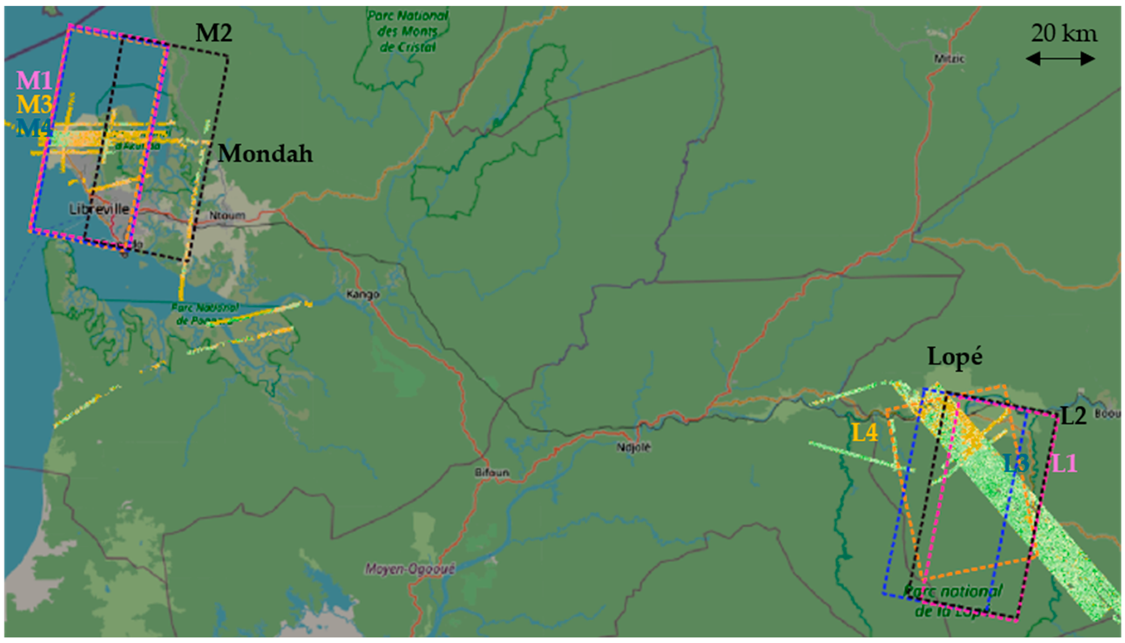
3. Experimental Data

Experimental data collected over two tropical forest sites, Mondah and Lopé, both located in Gabon (see Figure 1), have been used in this study. The Mondah site is a protected coastal forest with relatively flat topography located near the capital of Libreville. The forest is partially flooded and consists of very heterogeneous stands of variable tree height and density, including mature stands with trees above 40 m, degraded stands, mangroves, and woodlands. The Lopé site is located within Lopé National Park in central Gabon. It is characterised by a more diverse landscape of hilly terrain with local slopes exceeding 20°, and includes savannah and dense colonizing rainforest stands with large trees up to 55 m high and high biomass levels.

Interferometric X-band data (9.8 GHz) with 100 MHz bandwidth data were acquired by TanDEM-X in a stripmap HH-polarisation mode with an average incidence angle of 40°. The acquisitions over the two sites were performed between 2010 and 2019 with vertical wavenumbers varying from 0.06 to 0.13 rad/m, corresponding to ambiguity heights (e.g., the height associated with a 2π interferometric phase difference) of 50 to 140 m (see

Table 1. TanDEM-X acquisition parameters for the two sites.

ID	TanDEM-X Acquisition ID: TDM1_SAR__COS_BIST_SM_S_SRA_	Test Site	${\mathbf{k}}_{\mathbf{z}}$ [rad/m]	Ambiguity Height [m]	Orbit
L1	20101231T045618_20101231T045626	Lopé	0.131	48.0	Desc
L2	20111002T045625_20111002T045633	Lopé	0.076	82.7	Desc
L3	20121215T045627_20121215T045635	Lopé	0.068	92.4	Desc
L4	20160125T173041_20160125T173048	Lopé	0.100	62.8	Asc
M1	20151111T050508_20151111T050516	Mondah	0.062	101.3	Desc
M2	20161211T050516_20161211T050524	Mondah	0.052	120.8	Desc
M3	20171117T050524_20171117T050532	Mondah	0.123	51.1	Desc
M4	20190704T050534_20190704T050542	Mondah	0.123	51.1	Desc

and Figure 1) along descending and ascending orbits. The TanDEM-X Coregistered Slant Range Single Look Complex (Co-SSC) data have been used to produce 100-look complex interferometric coherence data, geocoded in the latitude/longitude coordinate system. The volumetric decorrelation was calculated from interferometric coherence after compensating for additive noise decorrelation, whereas temporal decorrelation and various system-induced decorrelations were assumed to be negligible.

Lidar full waveform data were collected during the AfriSAR2016 campaign in February 2016 by NASA’s LVIS airborne lidar configuration. The footprints of LVIS returns range from 18 to 22 m, and the waveforms were resampled to a regular 20 m × 20 m grid with corresponding RH100 and DTM models provided by [8] and shown in Figure 2 and Figure 3.

A 20 m × 20 m forest-non-forest map has been used to mask out the non-forested regions as well as water and settlements in the two sites (see Figure 2 and Figure 3) [41].

4. Results

4.1. General Reconstruction Performance

In this section, the two sets of basis functions, Legendre and lidar-derived eigen-profiles, are compared in terms of their performance to reconstruct the vertical X-band reflectivity profile. The eigen-profiles are obtained from the available lidar waveforms for trees with heights ranging from 40 to 45 m following the approach proposed in [29] and outlined in the previous section. As outlined in Section 2, the range of heights for waveform selection in $\left[\mathrm{P}\right]$ can be defined for a certain height range within the forest sites. As both the Lopé and Mondah sites contain a large number of stands above 40 m, the matrix $\left[\mathrm{P}\right]$ contains a sufficiently large number of samples to produce a statistically meaningful matrix $\left[\mathrm{R}\right]$.

Figure 4 displays the first five lidar eigen-profiles for the Lopé (green curves) and the Mondah (orange curves) sites alongside the conventional Legendre functions (blue curves). The zeroth-order eigen-profiles, i.e., the ones corresponding to the largest eigenvalue, provide a low-frequency representation of the mean scattering contributions at the different heights. Common to both sites, they indicate that most of the scattering contributions are localised at the higher levels, as expected at the X-band. The higher-order profiles capture higher-frequency components of the vertical reflectivity function along the height. The similarity of the lower-order eigen-profiles across the two sites is visually apparent, despite the significantly different forest structural conditions. The site difference is reflected in the higher-order eigen-profiles, which become less similar.

The top row of Figure 5 shows the lidar waveforms along a transect aligned with the 0.85 latitude line in the Mondah site. The waveforms are decomposed (by means of (6)) into both function bases, the Legendre and the eigen-profile bases, and then reconstructed using only the first three components of each basis. The three-component reconstruction in the Legendre basis is shown in the second row of Figure 5, while the three-component reconstruction in the eigen-profile basis is shown in the third row. The three-component reconstruction in the eigen-profile basis appears to have a higher vertical resolution, providing a more detailed approximation of the original waveform than the three-component reconstruction in the Legendre basis.

In order to further investigate the reconstruction accuracy quantitatively, the number of basis functions required to represent 80% of the reflectivity of the lidar waveform is estimated in both bases. The obtained results are shown in Figure 6, for the Legendre basis on the top and the eigen-profile basis on the bottom. The eigen-profile basis proves more effective in representing the lidar waveforms with a lower number of functions compared to the Legendre basis, especially for tall stands: three to four eigen-profiles are sufficient, while five to six Legendre functions are required. Meanwhile, for lower stands, the number of required Legendre functions is either similar or even smaller.

4.2. Single-Baseline Reconstruction

For the single-baseline PCT reconstruction, the same TanDEM-X acquisition has been used for both basis sets. In order to establish a criterion for assessing the reconstruction quality, the reconstructed vertical reflectivity profile ${\mathrm{f}}_{\mathrm{P}\mathrm{C}\mathrm{T}}\left(\mathrm{z}\right)$ is used in (3) to model the volumetric decorrelation for the available vertical wavenumbers ${\mathrm{k}}_{\mathrm{z}}^{\mathrm{m}}$ as [42]

$${\tilde{\mathsf{\gamma }}}_{\mathrm{V}\mathrm{o}\mathrm{l},\mathrm{M}\mathrm{o}\mathrm{d}}^{\mathrm{m}}\left({\mathrm{k}}_{\mathrm{z}}^{\mathrm{m}}\right)=\frac{{\int }_0^1{\mathrm{f}}_{\mathrm{P}\mathrm{C}\mathrm{T}}\left(\mathrm{z}\right)\mathrm{e}\mathrm{x}\mathrm{p}\left(\mathrm{j}{\mathrm{k}}_{\mathrm{Z}}^{\mathrm{m}}{\mathrm{h}}_{\mathrm{v}}^{\mathrm{r}\mathrm{e}\mathrm{f}}\mathrm{z}\right)\mathrm{d}\mathrm{z}}{{\int }_0^1{\mathrm{f}}_{\mathrm{P}\mathrm{C}\mathrm{T}}\left(\mathrm{z}\right)\mathrm{d}\mathrm{z}}.$$

(19)

The modelled ${\tilde{\mathsf{\gamma }}}_{\mathrm{V}\mathrm{o}\mathrm{l},\mathrm{M}\mathrm{o}\mathrm{d}}^{\mathrm{m}}$ are then compared to the measured ones, ${\tilde{\mathsf{\gamma }}}_{\mathrm{V}\mathrm{o}\mathrm{l}}^{\mathrm{m}}$, at the same vertical wavenumbers. The quality of the matching serves as an indicator of the quality of the reconstructed vertical reflectivity profile. A comparison of this matching at different vertical wavenumbers, e.g., for different observations, obviously assumes the profile to remain unchanged across observations. For a quantitative assessment of the matching between modelled and measured volume absolute volumetric decorrelation values, the bias, the root mean square error (RMSE) and the correlation coefficient ${\mathrm{r}}^2$ are used

$$\begin{gathered} {\mathrm{B}\mathrm{i}\mathrm{a}\mathrm{s}}_{\mathrm{m}}=\frac{1}{\mathrm{Q}}{\sum }_{\mathrm{q}}\left({\left|{\tilde{\mathsf{\gamma }}}_{\mathrm{V}\mathrm{o}\mathrm{l},\mathrm{M}\mathrm{o}\mathrm{d}}^{\mathrm{m}}\right|}_{\mathrm{q}}-{\left|{\tilde{\mathsf{\gamma }}}_{\mathrm{V}\mathrm{o}\mathrm{l}}^{\mathrm{m}}\right|}_{\mathrm{q}}\right) \\ {\mathrm{R}\mathrm{M}\mathrm{S}\mathrm{E}}_{\mathrm{m}}=\frac{1}{\mathrm{Q}}\sqrt{{\sum }_{\mathrm{q}}{\left({\left|{\tilde{\mathsf{\gamma }}}_{\mathrm{V}\mathrm{o}\mathrm{l},\mathrm{M}\mathrm{o}\mathrm{d}}^{\mathrm{m}}\right|}_{\mathrm{q}}-{\left|{\tilde{\mathsf{\gamma }}}_{\mathrm{V}\mathrm{o}\mathrm{l}}^{\mathrm{m}}\right|}_{\mathrm{q}}\right)}^2} \\ {\mathrm{r}}_{\mathrm{m}}^2=1-\frac{{\sum }_{\mathrm{q}}{\left({\left|{\tilde{\mathsf{\gamma }}}_{\mathrm{V}\mathrm{o}\mathrm{l},\mathrm{M}\mathrm{o}\mathrm{d}}^{\mathrm{m}}\right|}_{\mathrm{q}}-{\left|{\tilde{\mathsf{\gamma }}}_{\mathrm{V}\mathrm{o}\mathrm{l}}^{\mathrm{m}}\right|}_{\mathrm{q}}\right)}^2}{{\sum }_{\mathrm{q}}{\left({\left|{\tilde{\mathsf{\gamma }}}_{\mathrm{V}\mathrm{o}\mathrm{l},\mathrm{M}\mathrm{o}\mathrm{d}}^{\mathrm{m}}\right|}_{\mathrm{q}}-\overline{\left|{\tilde{\mathsf{\gamma }}}_{\mathrm{V}\mathrm{o}\mathrm{l},\mathrm{M}\mathrm{o}\mathrm{d}}^{\mathrm{m}}\right|}\right)}^2} \end{gathered}$$

(20)

where $\overline{\left|{\tilde{\mathsf{\gamma }}}_{\mathrm{V}\mathrm{o}\mathrm{l},\mathrm{M}\mathrm{o}\mathrm{d}}^{\mathrm{m}}\right|}$ is the mean modelled volume absolute volumetric decorrelation value, and Q is the number of PCT estimated vertical reflectivity profiles.

Figure 7 shows the X-band reconstructed vertical reflectivity profiles in Mondah, using the acquisition M1 with the Legendre basis (top row) and the eigen-profile basis (bottom row). In the eigen-profile basis reconstruction the scattering contributions, identified in correspondence with the local maxima of the reconstructed vertical reflectivity profile, are more concentrated on the higher canopy layer. Meanwhile, in the Legendre basis, they appear more distributed across a wider (and lower) height range.

Figure 8 shows the reconstruction performance for the Mondah site. The vertical reflectivity profiles have been reconstructed from acquisition M1 (see Table 1). The correlation histograms indicate the correspondence between the measured and modelled volumetric decorrelation for the acquisitions M1–M4. The results obtained using the Legendre basis are on the top row, while the results obtained using the eigen-profile basis are on the bottom row. Clearly, the measured volumetric decorrelation matches the modelled one for the acquisition M1, i.e., the same one which was used to produce the PCT vertical reflectivity profiles. For the other interferometric acquisitions M2–M4, discrepancies exist depending on the vertical wavenumber and the type of basis employed. The RMSE varies from 0.1 for the similar vertical wavenumber (though with higher volumetric decorrelation on average) to 0.2 for significantly larger vertical wavenumbers. The ${\mathrm{r}}^2$ value is below 0.1 for both basis types, with a slightly better correlation in the Legendre basis case, while the mean bias is smaller for the eigen-profile basis.

A similar analysis for Lopé is presented in Figure 9, where acquisition L2 was used for the reconstruction of the vertical reflectivity profiles. Unlike the Mondah acquisitions, which all are performed in descending orbits, the Lopé data set includes one ascending orbit (L4). Across the descending orbits, the RMSE varies from 0.12 to 0.24, with slightly better performance for eigen-profile basis reconstruction. For the ascending orbit, the correlation breaks down with ${\mathrm{r}}^2$ not exceeding 0.01.

4.3. Dual-Baseline Reconstruction

The natural extension is to add more interferometric observations at different vertical wavenumbers in the PCT reconstruction, aiming for the reconstruction of higher-frequency components of the vertical reflectivity profile. In Figure 10, the dual-baseline reconstructed vertical reflectivity profiles in Mondah are presented, using the acquisitions M1 and M3, with the Legendre basis (top row) and the eigen-profile basis (bottom row). Figure 11 presents the corresponding correlation histograms. Evidently, the two InSAR acquisitions used to derive the PCT vertical reflectivity profile show the best correlation between measured and modelled volumetric decorrelations. However, no significant difference in performance between the two bases is observed.

This is a consequence of poor conditioning of (9), which can be addressed by applying a regularization on the matrix [F]. The regularisation can be done either through a diagonal loading of the matrix [F] or through a matrix filtering employed by removing the lowest singular value(s) component from the matrix $\left[\mathsf{\Sigma }\right]$ in (10) [21]. In the second case, the conditioning number (CN) is determined by the second smallest singular value. The second approach is used for the dual-baseline matrix regularisation.

Figure 12 demonstrates the effect of regularisation of the [F] matrix, applied through matrix filtering, on the CN for both the Legendre and the eigen-profile basis. The theoretical structure of matrix [F] is studied. The dual-baseline results using ${\mathrm{k}}_{\mathrm{V}}^1$ and ${\mathrm{k}}_{\mathrm{V}}^2$ with small CN are the ones where noise has a lesser effect on the reconstruction performance. For the given $4\times 4$ matrix the CN varies from 1 (well-conditioned) to more than ${10}^5$ (ill-conditioned). The Legendre matrix [${\mathrm{F}}^{\mathrm{L}}$] does not depend on the measured volumetric decorrelation, whereas a general matrix [F] depends on the measured volumetric decorrelation. This is reflected in the specific high CN features of the CN plot for the matrix [F], which, notably, disappears after applying the matrix regularisation.

Accordingly, dual-baseline reconstruction allows a more accurate with higher vertical resolution reconstruction expressed through the ability to interpret a wider range of vertical wavenumbers. However, the ill-conditioned multi-baseline problem can lead to erroneous reconstructions.

5. Discussion

The use of an eigen-profile basis allows a vertical reflectivity profile reconstruction that is better adapted to certain forest conditions compared to the use of the Legendre polynomials. Acting as principal components in the lidar waveform, they converge to the original waveform with only a few components, as visualised in Figure 5. Indeed, as demonstrated by Figure 6, for taller forest stands, 3–4 eigen-profiles appear sufficient to represent 80% of the energy of the lidar waveforms, compared to 5–6 required in the Legendre basis. A qualitative evaluation of the reconstructed vertical reflectivity profiles reveals that the eigen-profile basis allows for a more realistic profile reconstruction when only a small number of components are available. Figure 7 shows that the eigen-profile basis reconstruction localises most of the X-band relative intensity in the top layer of the canopy, while the Legendre basis tends to distribute the relative intensity over a larger height range and towards the middle layer. However, in the absence of reference 3D radar reflectivity measurements, such as those obtained by tomographic SAR measurements, a direct assessment of the accuracy of the reconstructed vertical reflectivity profiles is not possible.

In order to establish an indirect quality criterion, the estimated PCT profiles were used to model the absolute volumetric decorrelation at various vertical wavenumbers. An accurately reconstructed profile should be capable of predicting volumetric decorrelations at any other vertical wavenumber with comparable incidence angles. This approach was applied to both single- and dual-baseline reconstruction scenarios to compare the PCT reconstruction performance of the two basis types.

In the single-baseline scenario, the PCT-reconstructed vertical reflectivity profile using the eigen-profile basis allowed the volumetric decorrelations to be modelled more accurately in terms of mean bias, compared to the Legendre basis, across the given vertical wavenumber range. The ${\mathrm{r}}^2$ value is comparable for both basis types, with a slightly better correlation of the Legendre basis in the Mondah test site. Notably, for similar vertical wavenumbers as those used for the PCT reconstruction, the error in modelling the volumetric decorrelation is low in both the Legendre and eigen-profile bases. The deviations increase when the comparison is performed for acquisitions with significantly different vertical wavenumbers than the ones used for the reconstruction. It is also evident that the vertical reflectivity profiles derived from different look directions cannot be directly compared, especially in sloped areas. As confirmed by Figure 11, the vertical reflectivity profiles from the descending orbit could not be correlated with volumetric decorrelation measurements from the ascending orbit.

The dual-baseline reconstruction allows a better reconstruction, expressed in the extended range of vertical wavenumbers where the reconstructed PCT vertical reflectivity profiles can correctly model the volumetric decorrelation. It also allows the higher-resolution features and structural components which are visible in the lidar reference to be resolved. However, the condition number of dual-baseline reconstruction is generally smaller compared to the single-baseline case, necessitating matrix regularisation. Careful consideration of baseline selection, as well as matrix regularisation, is mandatory to achieve physically significant results in the multi-baseline scenario.

When the temporal separation between interferometric acquisitions becomes large, changes in reflectivity induced by changes in dielectric and, structural conditions cannot be neglected anymore. This makes single-baseline PCT reconstructions more attractive for large-scale spaceborne applications, resulting in a more critical choice of the basis for an accurate reconstruction.

The applicability of certain lidar-based eigen-profile bases to specific forest compositions and terrains is limited by differences between radar and lidar vertical reflectivity profiles, potential errors in lidar waveform reconstructions, and the inability to account for the full range of profile diversity within a given forest type. Additionally, it is expected that in sloped areas, the performance of PCT reconstruction could be reduced not only by errors in the terrain elevation estimation but also by inaccurate basis representation, for instance if basis functions were derived solely in flat terrains. Nevertheless, the use of an eigen-profile basis allows for adaptation to the chosen scenario, which is especially useful when only a small set of interferometric acquisitions is available.

6. Conclusions

In this paper, the performance of two different basis types to reconstruct the X-band vertical reflectivity profile by means of single- and dual-baseline PCT at various interferometric baselines has been investigated. The reconstruction was tested at two different tropical forest sites, covering a wide range of forest stand and topographic conditions.

Lidar waveforms, even if only sparsely available, enable the determination of a set of orthogonal basis functions that can be used to expand the underlying reflectivity as a series. When used in the PCT framework, this eigen-profile basis enables a reconstruction of the vertical reflectivity of a specific forest by estimating the expansion coefficients from interferometric coherence measurements. The use of such a lidar-derived eigen-profile basis outperforms the originally proposed Legendre polynomial basis, especially in the single-baseline inversion scenario, where the ability of the first three basis functions to effectively represent the physical vertical reflectivity profile is critical.

The combination of a lidar-derived basis with interferometric SAR measurements establishes a framework to increase the synergy between missions such as TanDEM-X and GEDI. It may also allow to estimate the change of the PCT-reconstructed coefficients in time, reflecting the change in the dielectric and/or structural properties of the illuminated forest stands. The PCT with an eigen-profile basis approach can potentially be applied to other SAR spaceborne missions, such as ESA’s BIOMASS, which will provide P-band tomographic data sets in the first stage and interferometric data sets in the second stage of the mission. Its tomographic-reconstructed vertical reflectivity profiles derived in the first stage of the mission can be used as a basis for the following interferometric stage, enabling PCT reconstruction and PCT coefficient change monitoring.

References

1. Bohn, F.J.; Huth, A. The Importance of Forest Structure to Biodiversity–Productivity Relationships. R. Soc. Open Sci. 2017, 4, 160521. [Google Scholar]
2. Fischer, R.; Knapp, N.; Bohn, F.; Shugart, H.H.; Huth, A. The Relevance of Forest Structure for Biomass and Productivity in Temperate Forests: New Perspectives for Remote Sensing. Surv. Geophys. 2019, 40, 709–734. [Google Scholar] [CrossRef]
3. Rödig, E.; Cuntz, M.; Rammig, A.; Fischer, R.; Taubert, F.; Huth, A. The Importance of Forest Structure for Carbon Fluxes of the Amazon Rainforest. Environ. Res. Lett. 2018, 13, 054013. [Google Scholar] [CrossRef]
4. Frolking, S.; Palace, M.W.; Clark, D.B.; Chambers, J.Q.; Shugart, H.H.; Hurtt, G.C. Forest Disturbance and Recovery: A General Review in the Context of Spaceborne Remote Sensing of Impacts on Aboveground Biomass and Canopy Structure. J. Geophys. Res. 2009, 114, 2008JG000911. [Google Scholar] [CrossRef]
5. Smith, R.I.; Schreuder, H.T.; Gregoire, T.G.; Wood, G.B. Sampling Methods for Multiresource Forest Inventory. Biometrics 1994, 50, 1235. [Google Scholar] [CrossRef]
6. Dubayah, R.O.; Drake, J.B. Lidar Remote Sensing for Forestry. J. For. 2000, 98, 44–46. [Google Scholar]
7. Asner, G.P.; Mascaro, J.; Muller-Landau, H.C.; Vieilledent, G.; Vaudry, R.; Rasamoelina, M.; Hall, J.S.; Van Breugel, M. A Universal Airborne LiDAR Approach for Tropical Forest Carbon Mapping. Oecologia 2012, 168, 1147–1160. [Google Scholar] [CrossRef]
8. Blair, J.; Hofton, M. AfriSAR LVIS L2 Geolocated Surface Elevation Product, Version 1; NASA National Snow and Ice Data Center Distributed Active Archive Center: Boulder, CO, USA.
9. Dubayah, R.; Blair, J.B.; Goetz, S.; Fatoyinbo, L.; Hansen, M.; Healey, S.; Hofton, M.; Hurtt, G.; Kellner, J.; Luthcke, S.; et al. The Global Ecosystem Dynamics Investigation: High-Resolution Laser Ranging of the Earth’s Forests and Topography. Sci. Remote Sens. 2020, 1, 100002. [Google Scholar] [CrossRef]
10. Yang, W.; Ni-Meister, W.; Lee, S. Assessment of the Impacts of Surface Topography, off-Nadir Pointing and Vegetation Structure on Vegetation Lidar Waveforms Using an Extended Geometric Optical and Radiative Transfer Model. Remote Sens. Environ. 2011, 115, 2810–2822. [Google Scholar] [CrossRef]
11. Del Río, M.; Pretzsch, H.; Alberdi, I.; Bielak, K.; Bravo, F.; Brunner, A.; Condés, S.; Ducey, M.J.; Fonseca, T.; Von Lüpke, N.; et al. Characterization of the Structure, Dynamics, and Productivity of Mixed-Species Stands: Review and Perspectives. Eur. J. For. Res. 2016, 135, 23–49. [Google Scholar] [CrossRef]
12. Pardini, M.; Armston, J.; Qi, W.; Lee, S.K.; Tello, M.; Cazcarra Bes, V.; Choi, C.; Papathanassiou, K.P.; Dubayah, R.O.; Fatoyinbo, L.E. Early Lessons on Combining Lidar and Multi-Baseline SAR Measurements for Forest Structure Characterization. Surv. Geophys. 2019, 40, 803–837. [Google Scholar] [CrossRef]
13. Reigber, A.; Moreira, A. First Demonstration of Airborne SAR Tomography Using Multibaseline L-Band Data. IEEE Trans. Geosci. Remote Sens. 2000, 38, 2142–2152. [Google Scholar] [CrossRef]
14. Lombardini, F.; Reigber, A. Adaptive Spectral Estimation for Multibaseline SAR Tomography with Airborne L-Band Data. In Proceedings of the IGARSS 2003. In Proceedings of the 2003 IEEE International Geoscience and Remote Sensing Symposium, Toulouse, France, 21–25 July 2003; Proceedings (IEEE Cat. No.03CH37477). IEEE: Toulouse, France, 2003; Volume 3, pp. 2014–2016. [Google Scholar]
15. Dubois-Fernandez, P.C.; Le Toan, D.S.; Oriot, H.; Chave, J.; Blanc, L.; Villard, L.; Davidson, M.W.J.; Petit, M. The TropiSAR Airborne Campaign in French Guiana: Objectives, Description, and Observed Temporal Behavior of the Backscatter Signal. IEEE Trans. Geosci. Remote Sens. 2012, 50, 3228–3241. [Google Scholar] [CrossRef]
16. Pardini, M.; Tello, M.; Cazcarra-Bes, V.; Papathanassiou, K.P.; Hajnsek, I. L-and P-Band 3-D SAR Reflectivity Profiles versus Lidar Waveforms: The AfriSAR Case. IEEE J. Sel. Top. Appl. Earth Obs. Remote Sens. 2018, 11, 3386–3401. [Google Scholar]
17. Frey; E. Meier Analyzing Tomographic SAR Data of a Forest with Respect to Frequency, Polarization, and Focusing Technique. IEEE Trans. Geosci. Remote Sens. 2011, 49, 3648–3659. [Google Scholar] [CrossRef]
18. Nannini, M.; Martone, M.; Rizzoli, P.; Prats-Iraola, P.; Rodriguez-Cassola, M.; Reigber, A.; Moreira, A. Coherence-Based SAR Tomography for Spaceborne Applications. Remote Sens. Environ. 2019, 225, 107–114. [Google Scholar] [CrossRef]
19. V. Cazcarra-Bes; M. Pardini; M. Tello; K. P. Papathanassiou Comparison of Tomographic SAR Reflectivity Reconstruction Algorithms for Forest Applications at L-Band. IEEE Trans. Geosci. Remote Sens. 2020, 58, 147–164. [Google Scholar] [CrossRef]
20. Cloude, S.R. Polarization Coherence Tomography. Radio Sci. 2006, 41, 1–27. [Google Scholar] [CrossRef]
21. Cloude, S.R. Dual-Baseline Coherence Tomography. IEEE Geosci. Remote Sens. Lett. 2007, 4, 127–131. [Google Scholar] [CrossRef]
22. Cloude, S. Polarisation: Applications in Remote Sensing; Oxford University Press: Oxford, UK, 2009; ISBN 978-0-19-956973-1. [Google Scholar]
23. Poorazimy, M.; Shataee, S.; Aghababaei, H.; Tomppo, E.; Praks, J. First Demonstration of Space-Borne Polarization Coherence Tomography for Characterizing Hyrcanian Forest Structural Diversity. Remote Sens. 2023, 15, 555. [Google Scholar]
24. Zhao, R.; Cao, S.; Zhu, J.; Fu, L.; Xie, Y.; Zhang, T.; Fu, H. A Dual-Baseline PolInSAR Method for Forest Height and Vertical Profile Function Inversion Based on the Polarization Coherence Tomography Technique. Forests 2023, 14, 626. [Google Scholar]
25. Praks, J.; Kugler, F.; Hyyppa, J.; Papathanassiou, K.; Hallikainen, M. SAR Coherence Tomography for Boreal Forest with Aid of Laser Measurements. In Proceedings of the IGARSS 2008—2008 IEEE International Geoscience and Remote Sensing Symposium, Boston, MA, USA, 7 July 2008; Volume 2, p. II–469. [Google Scholar]
26. Krieger, A.; Moreira, H.; Fiedler, I.; Hajnsek, M.; Werner, M.; Younis, M. Zink TanDEM-X: A Satellite Formation for High-Resolution SAR Interferometry. IEEE Trans. Geosci. Remote Sens. 2007, 45, 3317–3341. [Google Scholar] [CrossRef]
27. Quegan, S.; Le Toan, T.; Chave, J.; Dall, J.; Exbrayat, J.-F.; Minh, D.H.T.; Lomas, M.; D’Alessandro, M.M.; Paillou, P.; Papathanassiou, K.; et al. The European Space Agency BIOMASS Mission: Measuring Forest above-Ground Biomass from Space. Remote Sens. Environ. 2019, 227, 44–60. [Google Scholar] [CrossRef]
28. Zhang, H.; Ma, P.; Wang, C. A New Function Expansion for Polarization Coherence Tomography. IEEE Geosci. Remote Sens. Lett. 2012, 9, 891–895. [Google Scholar] [CrossRef]
29. Guliaev, R.; Cazcarra-Bes, V.; Pardini, M.; Papathanassiou, K. Forest Height Estimation by Means of TanDEM-X InSAR and Waveform Lidar Data. IEEE J. Sel. Top. Appl. Earth Obs. Remote Sens. 2021, 14, 3084–3094. [Google Scholar]
30. Choi, C.; Cazcarra-Bes, V.; Guliaev, R.; Pardini, M.; Papathanassiou, K.P.; Qi, W.; Armston, J.; Dubayah, R.O. Large-Scale Forest Height Mapping by Combining TanDEM-X and GEDI Data. IEEE J. Sel. Top. Appl. Earth Obs. Remote Sens. 2023, 16, 2374–2385. [Google Scholar] [CrossRef]
31. Choi, C.; Pardini, M.; Armston, J.; Papathanassiou, K.P. Forest Biomass Mapping Using Continuous InSAR and Discrete Waveform Lidar Measurements: A TanDEM-X/GEDI Test Study. IEEE J. Sel. Top. Appl. Earth Obs. Remote Sens. 2023, 16, 7675–7689. [Google Scholar] [CrossRef]
32. Qi, W.; Armston, J.; Choi, C.; Stovall, A.; Saarela, S.; Pardini, M.; Fatoyinbo, L.; Papathanasiou, K.; Dubayah, R. Mapping Large-Scale Pantropical Forest Canopy Height by Integrating GEDI Lidar and TanDEM-X InSAR Data. 2023. Available online: https://www.researchsquare.com/article/rs-3306982/v1 (accessed on 20 May 2024).
33. Schlund, M.; Wenzel, A.; Camarretta, N.; Stiegler, C.; Erasmi, S. Vegetation Canopy Height Estimation in Dynamic Tropical Landscapes with TanDEM-X Supported by GEDI Data. Methods Ecol. Evol. 2023, 14, 1639–1656. [Google Scholar] [CrossRef]
34. Yu, Y.; Lei, Y.; Siqueira, P. Large-Scale Forest Height Mapping in the Northeastern U.S. Using L-Band Spaceborne Repeat-Pass SAR Interferometry and GEDI LiDAR Data. In Proceedings of the IGARSS 2023—2023 IEEE International Geoscience and Remote Sensing Symposium, Pasadena, CA, USA, 16 July 2023; pp. 1760–1763. [Google Scholar]
35. Lei, Y.; Siqueira, P.; Torbick, N.; Ducey, M.; Chowdhury, D.; Salas, W. Generation of Large-Scale Moderate-Resolution Forest Height Mosaic with Spaceborne Repeat-Pass SAR Interferometry and Lidar. IEEE Trans. Geosci. Remote Sens. 2018, 57, 770–787. [Google Scholar]
36. Treuhaft, R.N.; Chapman, B.D.; Dos Sãntos, J.R.; Gonçalves, F.G.; Dutra, L.V.; Graça, P.M.; Drake, J.B. Vegetation Profiles in Tropical Forests from Multibaseline Interferometric Synthetic Aperture Radar, Field, and Lidar Measurements. J. Geophys. Res. Atmos. 2009, 114. [Google Scholar] [CrossRef]
37. Fatoyinbo, T.; Armston, J.; Simard, M.; Saatchi, S.; Denbina, M.; Lavalle, M.; Hofton, M.; Tang, H.; Marselis, S.; Pinto, N.; et al. The NASA AfriSAR Campaign: Airborne SAR and Lidar Measurements of Tropical Forest Structure and Biomass in Support of Current and Future Space Missions. Remote Sens. Environ. 2021, 264, 112533. [Google Scholar] [CrossRef]
38. Hagberg, J.O.; Ulander, L.M.; Askne, J. Repeat-Pass SAR Interferometry over Forested Terrain. IEEE Trans. Geosci. Remote Sens. 1995, 33, 331–340. [Google Scholar]
39. Askne, J.I.; Dammert, P.B.; Ulander, L.M.; Smith, G. C-Band Repeat-Pass Interferometric SAR Observations of the Forest. IEEE Trans. Geosci. Remote Sens. 1997, 35, 25–35. [Google Scholar]
40. Chen, H.; Cloude, S.R.; White, J.C. Using GEDI Waveforms for Improved TanDEM-X Forest Height Mapping: A Combined SINC + Legendre Approach. Remote Sens. 2021, 13. [Google Scholar] [CrossRef]
41. Martone, M.; Rizzoli, P.; Wecklich, C.; González, C.; Bueso-Bello, J.-L.; Valdo, P.; Schulze, D.; Zink, M.; Krieger, G.; Moreira, A. The Global Forest/Non-Forest Map from TanDEM-X Interferometric SAR Data. Remote Sens. Environ. 2018, 205, 352–373. [Google Scholar] [CrossRef]
42. Hoekman, D.H.; Varekamp, C. Observation of Tropical Rain Forest Trees by Airborne High-Resolution Interferometric Radar. IEEE Trans. Geosci. Remote Sens. 2001, 39, 584–594. [Google Scholar] [CrossRef]
Figure 1. TanDEM-X scenes intersecting the lidar flights over Mondah and Lopé forests, overlaid with Open Street Map. Colour polygons identify different TanDEM-X acquisition extents.
Remotesensing 16 02146 g001
Figure 2. Mondah forest. From top to bottom: lidar RH100 and digital terrain model, forest-non-forest map.
Remotesensing 16 02146 g002
Figure 3. Lopé forest. From left to right: lidar RH100 and digital terrain model, forest-non-forest map.
Remotesensing 16 02146 g003
Figure 4. From left to right: basis function of zeroth to fourth order for Legendre (Blue), Mondah lidar eigen-profile basis (Orange), Lopé lidar eigen-profile basis (Green).
Remotesensing 16 02146 g004
Figure 5. Mondah forest vertical reflectivity profiles along 0.585 latitude from 9.31 to 9.37 longitude. From top to bottom: lidar waveforms, lidar waveforms decomposed on three coefficients of Legendre basis, lidar waveforms decomposed on three coefficients of eigen-profile basis. The vertical axis is relative to the LVIS DTM, i.e., zero corresponds to the elevation from DTM. Green curve corresponds to the LVIS RH100.
Remotesensing 16 02146 g005
Figure 6. Mondah forest. Number of functions to reconstruct 80% of lidar waveforms using Legendre basis (top) and eigen-profile basis (bottom).
Remotesensing 16 02146 g006
Figure 7. Mondah forest vertical reflectivity profiles along 0.585 latitude from 9.31 to 9.37 longitude. Single-baseline PCT reconstructed vertical reflectivity profiles using Legendre basis (top row) and eigen-profile basis (bottom row). The vertical axis is relative to the LVIS DTM, i.e., zero corresponds to the elevation from DTM. Green curve corresponds to the LVIS RH100. PCT vertical reflectivity profiles were reconstructed using acquisition M1.
Remotesensing 16 02146 g007
Figure 8. Mondah forest. Correlation histograms between measured and modelled volumetric decorrelation using single-baseline PCT reconstructed vertical reflectivity profile with Legendre (top row) and eigen-profile basis (bottom row). From left to right TanDEM-X acquisitions: M1–M4. Acquisition M1 was used to derive the single-baseline PCT vertical reflectivity profiles.
Remotesensing 16 02146 g008
Figure 9. Lopé forest. Correlation histograms between measured and modelled volumetric decorrelation using single-baseline PCT reconstructed vertical reflectivity profile with Legendre (top row) and eigen-profile basis (bottom row). From left to right TanDEM-X acquisitions: L1–L4. Acquisition L2 was used to reconstruct the single-baseline vertical reflectivity profile.
Remotesensing 16 02146 g009
Figure 10. Mondah forest vertical reflectivity profiles along 0.585 latitude from 9.31 to 9.37 longitude. Dual-baseline PCT reconstructed vertical reflectivity profiles using Legendre basis (top row) and eigen-profile basis (bottom row). The vertical axis is relative to the LVIS DTM, i.e., zero corresponds to the elevation from DTM. Green curve corresponds to the LVIS RH100. PCT vertical reflectivity profiles were reconstructed using acquisitions M1 and M3.
Remotesensing 16 02146 g010
Figure 11. Mondah forest. Correlation histograms between measured and modelled volumetric decorrelation using dual-baseline PCT vertical reflectivity profile with Legendre (top row) and eigen-profile basis (bottom row). From left to right are TanDEM-X acquisitions: M1–M4. Acquisitions M1 and M3 were used to reconstruct the dual-baseline vertical reflectivity profiles.
Remotesensing 16 02146 g011
Figure 12. Dual-baseline condition number of Legendre matrix (top row) and eigen-profile matrix (bottom row), not filtered (left column) and filtered (right column).
Remotesensing 16 02146 g012