Two-Dimensional Autofocus for Ultra-High-Resolution Squint Spotlight Airborne SAR Based on Improved Spectrum Modification

Abstract

For ultra-high-resolution (UHR) squint spotlight airborne synthetic aperture radar (SAR), the severe range-azimuth coupling caused by squint mode and the spatial and frequency dependence of the motion error brought by ultra-wide bandwidth both make it difficult to obtain satisfactory imaging results. Although some autofocus methods for squint airborne SAR have been presented in the published literature, their practical applicability in UHR situations remains limited. In this article, a new 2D wavenumber domain autofocus method combined with the Omega-K algorithm dedicated to UHR squint spotlight airborne SAR is proposed. First, we analyze the dependence of range envelope shift error (RESE) and range defocus on the squint angle and then propose a new spectrum modification strategy, after which the spectrum transforms into a quasi-side-looking one. The accuracy of estimation and compensation can be improved significantly in this way. Then, the 2D phase error can be calculated with the 1D estimated error by the mapping relationship, and after that the 2D compensation is performed in the wavenumber domain. Furthermore, the image-blocking technique and range-dependent motion error compensation method are embedded to accommodate the spatial-variant motion error for UHR cases. Simulations are carried out to verify the effectiveness of the proposed method.

1. Introduction

Synthetic aperture radar (SAR) is an active remote-sensing technique that can operate in several different modes [1,2]. With the developments over the past few decades, it can realize ultra-high-resolution (UHR) up to the centimeter level [3,4,5]. For UHR squint spotlight SAR, the squint mode is more flexible compared with the side-looking mode [6,7], and the UHR means more detailed information about the observation scenarios of interest. Although possessing many advantages, it is more challenging to process airborne UHR squint spotlight SAR data [8], for which the severe range-azimuth coupling introduced by the squint angle, and the spatial and frequency dependence of the motion error brought by the ultra-wide bandwidth, both place higher demands on the imaging process.

Due to the severe range-azimuth coupling of squint SAR, traditional SAR imaging algorithms, such as the range-Doppler algorithm (RDA) [9] and the chirp scaling algorithm (CSA) [10], are no longer applicable. Although some modified versions, for example, the squinted RDA [11], the nonlinear CSA (NCSA) [12,13], the extended NCS (ENCS) method [14,15], etc., have been proposed in the literature, they adopt different approximations, which still cannot satisfy the UHR situations. Besides the frequency-domain algorithms mentioned above, the back-projection algorithm (BPA) [16], as a time-domain algorithm, and the Omega-K algorithm ($\omega$KA) [17], as a wavenumber domain algorithm, are both considered to be the most accurate SAR imaging algorithms and can handle the squint SAR data with high accuracy. Since BPA is a point-by-point projection method, it is of great computational complexity and rather low efficiency. Therefore, in this article we adopt $\omega$KA as the imaging algorithm to obtain the coarse-focused image.

Different from the spaceborne SAR, which moves along a fixed orbit, the airborne SAR platform is subject to inevitable trajectory deviations. To obtain an accurately focused image, the slant range error should be limited within a fractional wavelength, which is generally not feasible with the provided positioning equipment, so in addition to motion compensation with the measured trajectory, it is necessary to estimate the error from the raw echo data, which is the autofocus process. Several autofocus methods have been proposed in the past few decades. They can be broadly classified into two categories: (1) the 1D autofocus methods that estimate and compensate the azimuth phase error (APE) based on parametric [18,19,20,21] or nonparametric methods [22,23,24,25,26]; (2) the 2D autofocus methods [27,28,29,30], which take into account not only the APE but also the range envelope shift error (RESE), and even the range defocus caused by higher-order errors along the range dimension.

On the one hand, for the UHR situation, the motion error will cause an obvious RESE that spans several or even dozens of range cells. In addition, the ultra-wide bandwidth makes the frequency dependence of the error non-negligible, which would otherwise cause defocus in the range dimension. Based on these considerations, 1D autofocus, which only considers the APE, cannot meet the requirements, and 2D autofocus is a better choice. On the other hand, for squint cases, it has been revealed in [31] that, with a non-negligible squint angle, even a small phase error will cause significantly amplified RESE after Omega-K imaging. To deal with this problem, several time-domain autofocus algorithms [31,32,33] are proposed, in which, they first perform azimuth deramping on the range downsampled data, and then compensate the residual azimuth-dependent phase terms by estimating the azimuth positions of the targets, after which the azimuth phase error can be estimated, and the motion error is retrieved and compensated on the raw echo data. In this way, both the APE and the amplified RESE are accounted for. However, the linear motion error will lead to a mismatch of the azimuth positions and further affect the accuracy of the subsequent phase error estimation [34]. Different from these time-domain algorithms, frequency-domain autofocus algorithms estimate the phase error in the azimuth-frequency domain [28,29], which avoids the deramp processing, thus circumventing the problem of azimuth position estimation, but the methods proposed in [28,29] are only suitable for side-looking or small squint mode, which cannot be directly used for squint cases. Recently, a novel frequency-domain autofocus algorithm tailored to squint SAR is proposed in [34]. However, the range defocus will affect the estimation accuracy of APE, especially for UHR cases, which is not mentioned in [34], and the approximation adopted during the azimuth alignment processing in [34] will also deteriorate the compensation result. The characteristics and limitations of the above methods are summarized in

Table 1. Comparison of current autofocus methods for UHR squint SAR.

	Time-Domain Methods [31,32,33]	Frequency-Domain Methods [34]
Characteristics	Needs deramp processing and azimuth position estimation; Compensation is applied to the raw data.	Avoids deramp processing and azimuth position estimation; Compensation is applied to the coarse-focused images.
Limitations	The estimation error of azimuth position will affect the subsequent estimation of phase error.	Lack of analysis of range defocus dependence on squint angles; Approximation adopted during azimuth alignment will deteriorate the compensation result.

.

To address the aforementioned issues, we present a novel 2D wavenumber domain autofocus method for UHR squint spotlight SAR in this article. First, with the approximated spectrum, we demonstrate that both the RESE and range defocus worsen as the squint angle increases. To improve the accuracy of the phase error estimation, a new spectrum modification strategy is proposed, which can alleviate the serious range defocus for squint cases and align the spectrum support regions. After spectrum modification, a 2D mapping of APE, which is deduced from the accurate spectrum, is used to compensate for the frequency-dependent phase error in the 2D wavenumber domain. Furthermore, to tackle the non-ignorable spatial variance of motion error for UHR cases, the image-blocking technique [35] and range-dependent motion error compensation methods [36] are embedded in the proposed method.

The remainder of this article is organized as follows. In Section 2.1, the signal model is established, and with the approximated spectrum the dependence of the phase error in the range-Doppler domain on the squint angle is analyzed. After that, the structure of the 2D phase error based on the accurate spectrum is derived. In Section 2.2, the spectrum modification strategy is introduced in detail, and the 2D phase error mapping after spectrum modification is discussed. Several simulation experiments are presented to verify the effectiveness of the proposed method in Section 3. Some discussions are presented in Section 4, and the conclusion is drawn in Section 5.

2. Materials and Methods

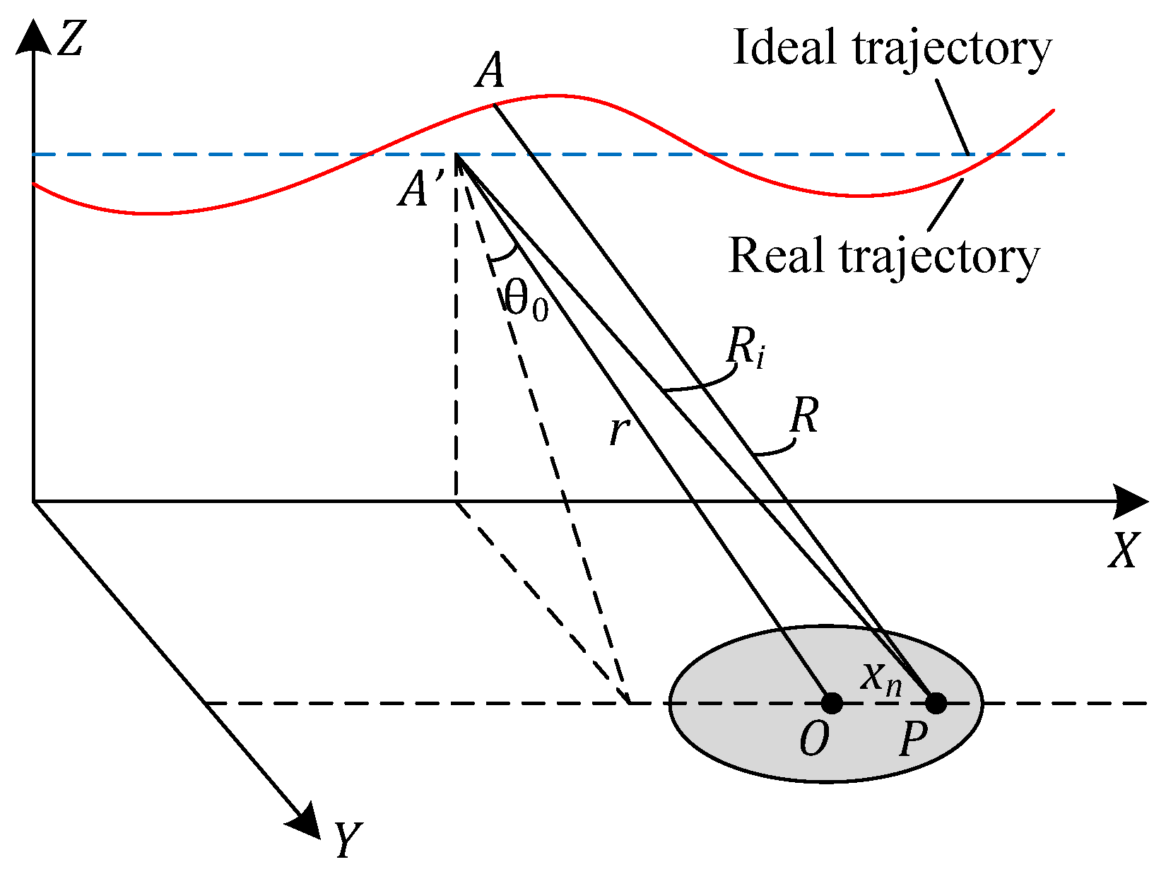
2.1. Signal Model and Problems Discussion

2.1.1. Signal Model

The geometric model of squint spotlight SAR is shown in Figure 1. The blue dashed line is the ideal trajectory and the red curved line denotes the real one affected by the motion error. The squint angle is ${\theta }_0$. r is the slant range from the aperture center to the scene center, O. Considering a target P located at the same range bin as O, the distance between P and O is $x_n$. The instantaneous range between the radar and P is

$$R\left(X\right)=R_i\left(X\right)+\Delta R\left(X\right)=\sqrt{{(rcos{\theta }_0)}^2+{(X-rsin{\theta }_0-x_n)}^2}+\Delta R\left(X\right),$$

(1)

where X is the azimuth position of the radar, $-\left(L/2\right)\le X\le \left(L/2\right)$, L is the aperture length, $R_i\left(X\right)$ denotes the ideal slant range, and $\Delta R\left(X\right)$ represents the slant range error caused by the motion error.

The demodulated received signal of target P can be expressed as

$$\begin{array}{c}\hfill ss(X,t)={\omega }_r\left(t-\frac{2R\left(X\right)}{c}\right){\omega }_a(X-x_n)·exp\left(j\pi k_r{\left(t-\frac{2R\left(X\right)}{c}\right)}^2\right)exp\left(-j\frac{4\pi f_0}{c}R\left(X\right)\right)\end{array},$$

(2)

where ${\omega }_r(·)$ is the envelope of the transmitted signal and ${\omega }_a(·)$ is the azimuth envelope decided by the antenna pattern function. t is the fast time, c is the speed of light, and $f_0$ and $k_r$ represent the carrier frequency and the frequency-modulated rate of the transmitted signal, respectively.

After range compression, the signal turns into

$$s{s}_1(X,t)=p_r\left(t-\frac{2R\left(X\right)}{c}\right){\omega }_a(X-x_n)exp\left(-j\frac{4\pi f_0}{c}R\left(X\right)\right),$$

(3)

where $p_r(·)$ is the range-compressed envelope (generally in a $\sin \mathrm{c}(·)$ form).

The range spectrum of (3) can be obtained by taking Fourier transform (FT) with respect to the fast time, t, which can be written as

$$sS(X,K_r)=W_r\left(K_r\right){\omega }_a(X-x_n)exp\left(-j{K}_{r}R\left(X\right)\right),$$

(4)

where $W_r(·)$ is the range envelope function in the wavenumber domain, $K_r=4\pi (f_0+f_r)/c$ is the range wavenumber, and $f_r$ is the range frequency.

Then, performing azimuth FT on (4) yields the 2D spectrum of target P, that is

$$\begin{array}{cc}\hfill SS(K_x,K_r)=& \int s{S}_1(X,K_r)exp(-j{K}_{x}X)dX\hfill \\ \hfill =& \int \begin{array}{c}{W}_r\left(K_r\right){\omega }_a(X-x_n)exp\left(-j{K}_{r}R\left(X\right)\right)·exp(-j{K}_{x}X)\hfill \end{array}dX\hfill \end{array}.$$

(5)

According to the principle of stationary phase (POSP), the stationary phase point can be calculated by setting the first-order derivative of the integrated phase of (5) to X to zero, i.e.,

$$\frac{d}{dX}\left(-K_{r}R\left(X\right)-K_{x}X\right)=0,$$

(6)

which can be turned into

$$-\frac{X-rsin{\theta }_0-x_n}{\sqrt{{(rcos{\theta }_0)}^2+{(X-rsin{\theta }_0-x_n)}^2}}-\frac{d\Delta R\left(X\right)}{dX}=\frac{K_x}{K_r}.$$

(7)

After solving the stationary phase point $X^{*}$ with (7) and inserting it into (5), we can obtain the expression of the 2D spectrum.

2.1.2. Negative Effects of Squint Angle

In this section, we discuss the negative effects of squint angle by analyzing the approximated spectrum of the signal.

With the ideal stationary point approximation, the stationary point can be solved from (7) as

$$X^{*}\approx -rcos{\theta }_0\frac{K_x}{\sqrt{K_r^2-K_x^2}}+x_n+rsin{\theta }_0.$$

(8)

Then, with (8), the 2D spectrum can be approximated as Equation (22) in [31],

$$S{S}_1(K_x,K_r)=W_x\left(K_x\right)·W_r\left(K_r\right)·exp\left(-j{K}_x{x}_n\right)·exp\left(-jrcos{\theta }_0\sqrt{K_r^2-K_x^2}-j{K}_{x}rsin{\theta }_0\right)·exp\left(-j{K}_r·\Delta R\left(X^{*}\right)\right),$$

(9)

where $K_x$ is the azimuth wavenumber and $W_x(·)$ represents the azimuth envelope function in the wavenumber domain.

Next, with conventional Stolt mapping [7], i.e., $K_y=\sqrt{K_r^2-K_x^2}$, the signal turns into

$$S{S}_2(K_x,K_y)=W_x\left(K_x\right)·W_y\left(K_y\right)·exp\left(-j{K}_x{x}_n\right)·exp\left(-j{K}_{y}rcos{\theta }_0-j{K}_{x}rsin{\theta }_0\right)·exp\left\{-j\sqrt{K_x^2+K_y^2}·\Delta R\left(X^{*}\right)\right\}.$$

(10)

The last term of (10) is the 2D phase error, that is

$${\Phi }_e(K_x,K_y)=-\sqrt{K_x^2+K_y^2}·\Delta R\left(X^{*}\right).$$

(11)

To further explore the relationship between the phase error and the squint angle, we perform Taylor series expansion on (11) with respect to range wavenumber $K_y$ at $K_y=K_{yc}$, that is,

$${\Phi }_e(K_x,K_y)={\varphi }_0\left(K_x\right)+{\varphi }_1\left(K_x\right)·(K_y-K_{yc})+{\varphi }_2\left(K_x\right)·{(K_y-K_{yc})}^2+\cdots ,$$

(12)

where ${\varphi }_0\left(K_x\right)$ denotes APE, ${\varphi }_1\left(K_x\right)$ represents the RESE, and ${\varphi }_2\left(K_x\right)$ and other higher-order terms account for the range defocus. To quantify the impact of the squint angle, we derive the values of coefficients ${\varphi }_1$ and ${\varphi }_2$ at the azimuth wavenumber center $K_x=K_{xc}$ as follows.

$${\varphi }_1\left(K_{xc}\right)\approx -cos{\theta }_0{\left.·\Delta R\left(X^{*}\right)\right|}_{K_y=K_{yc}}-r·\frac{sin{\theta }_0}{cos{\theta }_0}·{\left.\frac{\partial \Delta R\left(X^{*}\right)}{\partial X^{*}}\right|}_{K_y=K_{yc}}$$

(13)

$$\begin{array}{cc}\hfill {\varphi }_2\left(K_{xc}\right)\approx & -\frac{1}{2K_{yc}}·{sin}^2{\theta }_{0}cos{\theta }_0·{\left.\Delta R\left(X^{*}\right)\right|}_{K_y=K_{yc}}+{\left.\frac{1}{K_{yc}}\frac{r{sin}^3{\theta }_0}{cos{\theta }_0}·\frac{\partial \Delta R\left(X^{*}\right)}{\partial X^{*}}\right|}_{K_y=K_{yc}}\hfill \\ \hfill & -{\left.\frac{1}{2K_{yc}}·\frac{r^2{sin}^2{\theta }_0}{cos{\theta }_0}·\frac{{\partial }^2\Delta R\left(X^{*}\right)}{\partial {X^{*}}^2}\right|}_{K_y=K_{yc}}\hfill \end{array}$$

(14)

The detailed derivations are given in Appendix A.

To show the influence of squint angles intuitively, we conduct several simulations with the parameters given in

Table 2. Simulation parameters.

Parameters	Values
Carrier frequency	15.14 GHz
Bandwidth	5.72 GHz
Time width	10 us
Sampling frequency	2500 MHz
Synthetic aperture length	296.34 m
Pulse repetition frequency	3600 Hz
Center slant range	885 m
Velocity	67 m/s

. The trajectory deviation used for the simulation is extracted from a real flight history obtained by an airborne microwave photonic-assisted SAR system [3], as shown in Figure 2. Here, no motion compensation is applied. By setting different squint angles varying from 0 to ${30}^{\circ }$, we obtain corresponding range envelopes in the range-Doppler domain after range cell migration correction (RCMC), as shown in Figure 3.

For side-looking, ${\theta }_0=0$, so ${\varphi }_1\left(K_{xc}\right)$ is linearly dependent on $\Delta R\left(X^{*}\right)$ and ${\varphi }_2\left(K_{xc}\right)\approx 0$, according to (13) and (14). As shown in Figure 3a, the RESE is constricted in about 20 range cells, and no range defocus exists in the middle part. While in the squint case, ${\theta }_0\ne 0$; thus, ${\varphi }_1\left(K_{xc}\right)$ has an additional term, which means larger RESE, and ${\varphi }_2\left(K_{xc}\right)\ne 0$ anymore, which is consistent with Figure 3b–d, where the RESE is significantly larger and the range defocus appears in the middle part. As the squint angle increases, the RESE and range defocus become more severe, which will greatly degrade the estimation accuracy of RESE and APE during autofocus processing.

It should be noted that, although some approximations are made in the above analysis, the simulation results shown in Figure 3 are basically consistent with (13) and (14). Therefore, (13) and (14) can, to some extent, reflect the dependence of the phase error on the squint angle.

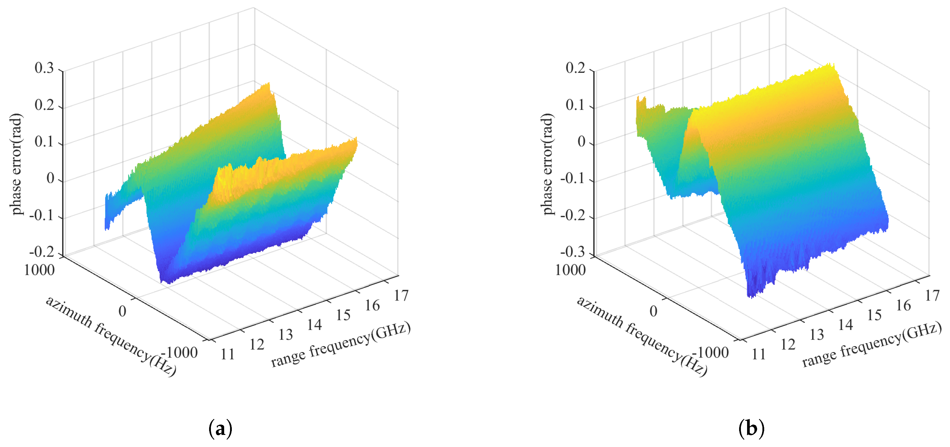
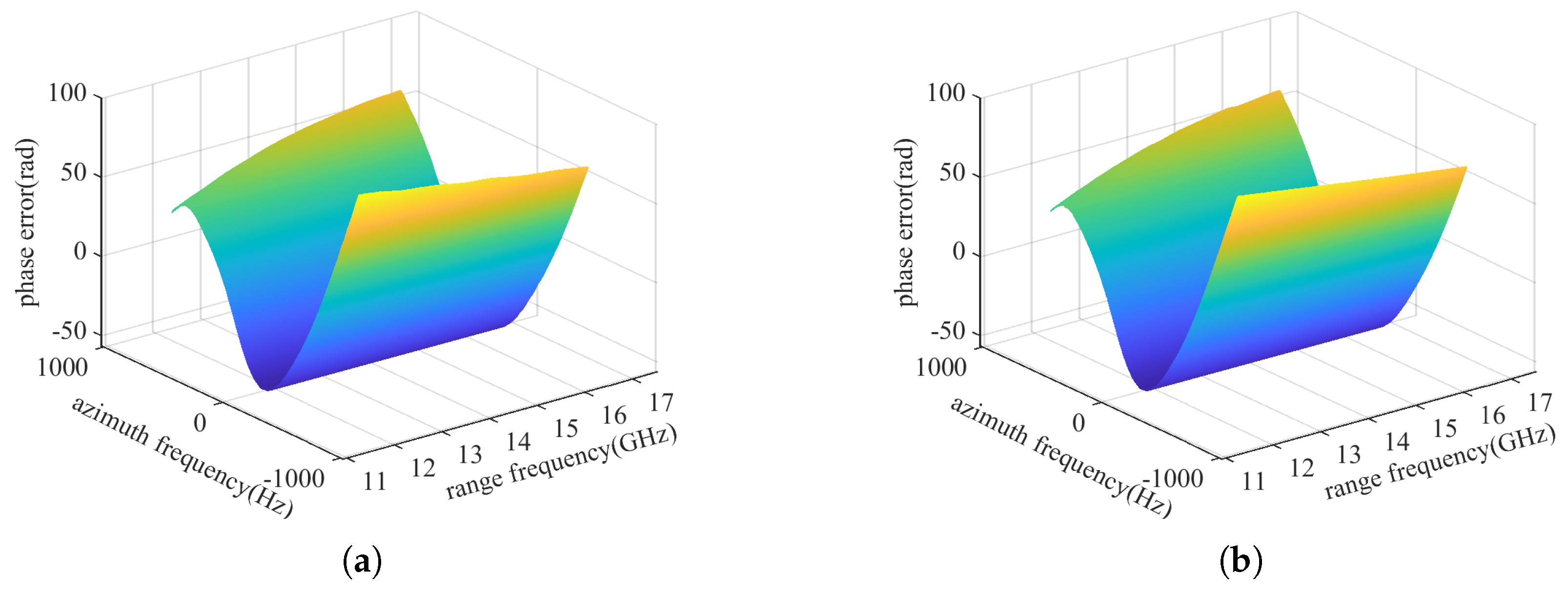
2.1.3. Accurate Structure of the 2D Phase Error

The 2D spectrum expressed in (9) is derived under the ideal stationary point approximation, which is intended to simplify the illustration of the negative influence of squint angles. However, for more accurate estimation and compensation of errors, it is necessary to derive a more accurate structure of the 2D phase error.

According to [28,34], the stationary point without approximation can be written in the following form, i.e.,

$$X^{*}=\xi \left(\frac{K_x}{K_r}\right)+rsin{\theta }_0+x_n,$$

(15)

where $\xi (·)$ is an unknown function that denotes the dependence of $X^{*}$ on $K_x$ and $K_r$.

Substituting (15) into (5) and using $\beta (·)$ to represent the composite function $R\left(X^{*}\left(·\right)\right)$, the spectrum without approximation can be written as

$$S{S}_3(K_x,K_r)=W_x\left(K_x\right)·W_r\left(K_r\right)·exp\left(-j{K}_x{x}_n\right)·exp\left\{-j{K}_r\beta \left(\frac{K_x}{K_r}\right)-j{K}_x\xi \left(\frac{K_x}{K_r}\right)\right\}·exp\left(-j{K}_{x}rsin{\theta }_0\right).$$

(16)

Then, again, substitute the conventional Stolt mapping $K_y=\sqrt{K_r^2-K_x^2}$ into (16), it turns into

$$\begin{array}{cc}\hfill S{S}_4(K_x,K_y)=& W_x\left(K_x\right)·W_y\left(K_y\right)·exp\left(-j{K}_x{x}_n\right)·exp\left(-j{K}_{x}rsin{\theta }_0\right)\hfill \\ \hfill & ·exp\left\{-j\sqrt{K_x^2+K_y^2}\beta \left(\frac{K_x}{\sqrt{K_x^2+K_y^2}}\right)\right\}·exp\left\{-j{K}_x\xi \left(\frac{K_x}{\sqrt{K_x^2+K_y^2}}\right)\right\}\hfill \end{array}.$$

(17)

Comparing (17) with the ideal spectrum, i.e., the first two exponential terms of (10), we can get the 2D error phase written as

$${\Phi }_e(K_x,K_y)=-\sqrt{K_x^2+K_y^2}\beta \left(\frac{K_x}{\sqrt{K_x^2+K_y^2}}\right)-K_x\xi \left(\frac{K_x}{\sqrt{K_x^2+K_y^2}}\right)+K_{y}rcos{\theta }_0.$$

(18)

It can also be written as

$${\Phi }_e(K_x,K_y)=K_y[-\sqrt{1+{\left(\frac{K_x}{K_y}\right)}^2}·\beta \left(\frac{\frac{K_x}{K_y}}{\sqrt{1+{\left(\frac{K_x}{K_y}\right)}^2}}\right)-\frac{K_x}{K_y}·\xi \left(\frac{\frac{K_x}{K_y}}{\sqrt{1+{\left(\frac{K_x}{K_y}\right)}^2}}\right)+rcos{\theta }_0].$$

(19)

Then, (19) can be simplified as

$${\Phi }_e(K_x,K_y)=K_y·\zeta \left(\frac{K_x}{K_y}\right),$$

(20)

where $\zeta (·)$ is defined as

$$\zeta \left(\nu \right)=-\sqrt{1+{\nu }^2}·\beta \left(\frac{\nu }{\sqrt{1+{\nu }^2}}\right)-\nu ·\xi \left(\frac{\nu }{\sqrt{1+{\nu }^2}}\right)+rcos{\theta }_0.$$

(21)

Therefore, although it is derived in the squint mode, the form of the 2D phase error, i.e., (20), is the same as that deduced in the side-looking mode in [28].

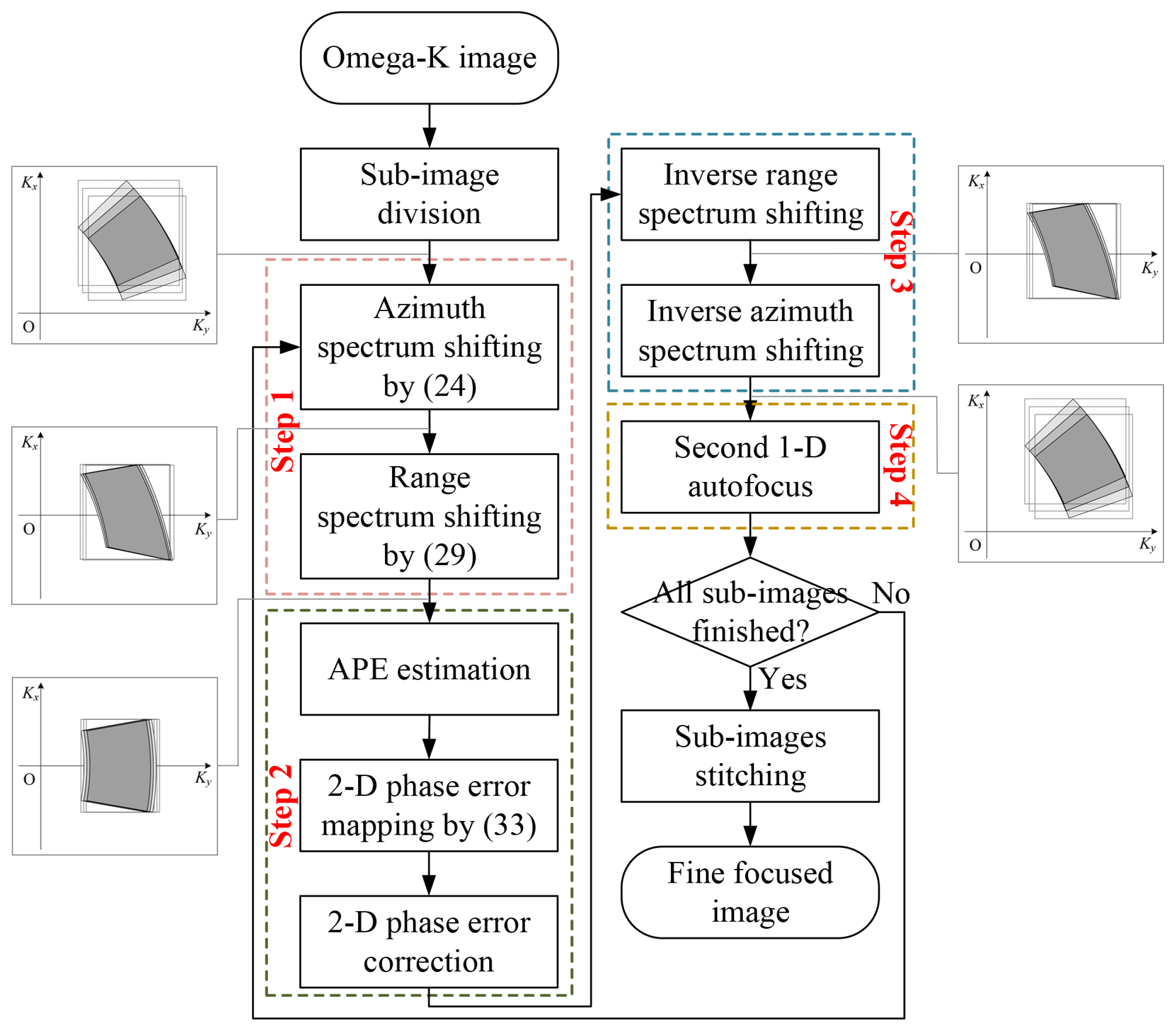
2.2. 2D Autofocus for UHR Squint Spotlight SAR

In this section, we propose a new 2D autofocus approach for UHR squint spotlight airborne SAR based on spectrum modification. According to the analysis in Section 2.1.2, under the same motion error both the RESE and range defocus deteriorate with increasing squint angles. Based on the previous conclusion and the subsequent analysis of the support region, we propose an improved spectrum modification strategy, in which the spectrum of the squint mode is transformed into a quasi-side-looking one. In this way, the range defocus can be greatly alleviated, and thus the estimation accuracy of RESE and APE can be greatly improved. Then, considering the frequency dependence of the phase error, we calculate the 2D phase error using the 2D mapping relationship deduced in Section 2.1.3 and compensate for it in the wavenumber domain.

2.2.1. Support Region Analysis

In fact, the analytical expressions of the 2D spectrum are the same for both side-looking and squint modes, as derived in Section 2.1.3. The main difference between the two modes lies in the support region of the wavenumber domain.

According to the geometric explanation, Chapter 8 in [2], the relationship between $K_x$ (the azimuth wavenumber), $K_r$ (the range wavenumber before Stolt mapping), and $K_y$ (the range wavenumber after Stolt mapping) can be written as

$$\left\{\begin{array}{c}{K}_x=K_{r}sin\theta \\ K_y=K_{r}cos\theta \end{array},\right.$$

(22)

where $\theta$ is the instantaneous squint angle. $K_r$ is determined only by the carrier frequency and bandwidth of the transmitted signal, while $K_x$ and $K_y$ are both affected by $K_r$ and the instantaneous squint angle. In side-looking mode, for a given target the squint angle at the synthetic aperture center is ${\theta }_c=0$, which implies that $K_x$ is symmetric about $K_x=0$ and $K_y$ is centered around $K_y=K_{rc}=4\pi f_0/c$. This means that the center of the support region $(K_{xc},K_{yc})$ is located at $(0,4\pi f_0/c)$. While for squint mode, ${\theta }_c\ne 0$; hence, the center of the support region $(K_{xc},K_{yc})$ will be displaced from $(0,4\pi f_0/c)$ to $(K_{rc}sin{\theta }_c,K_{rc}cos{\theta }_c)$.

Based on the above analysis about the support region, we propose the following spectrum modification strategy to convert the squint mode spectrum into a quasi-side-looking one, that is to say, shift the spectrum support region to make it change from a skew one centered at $K_x=K_{rc}sin{\theta }_c$ to a symmetric one centered at $K_x=0$.

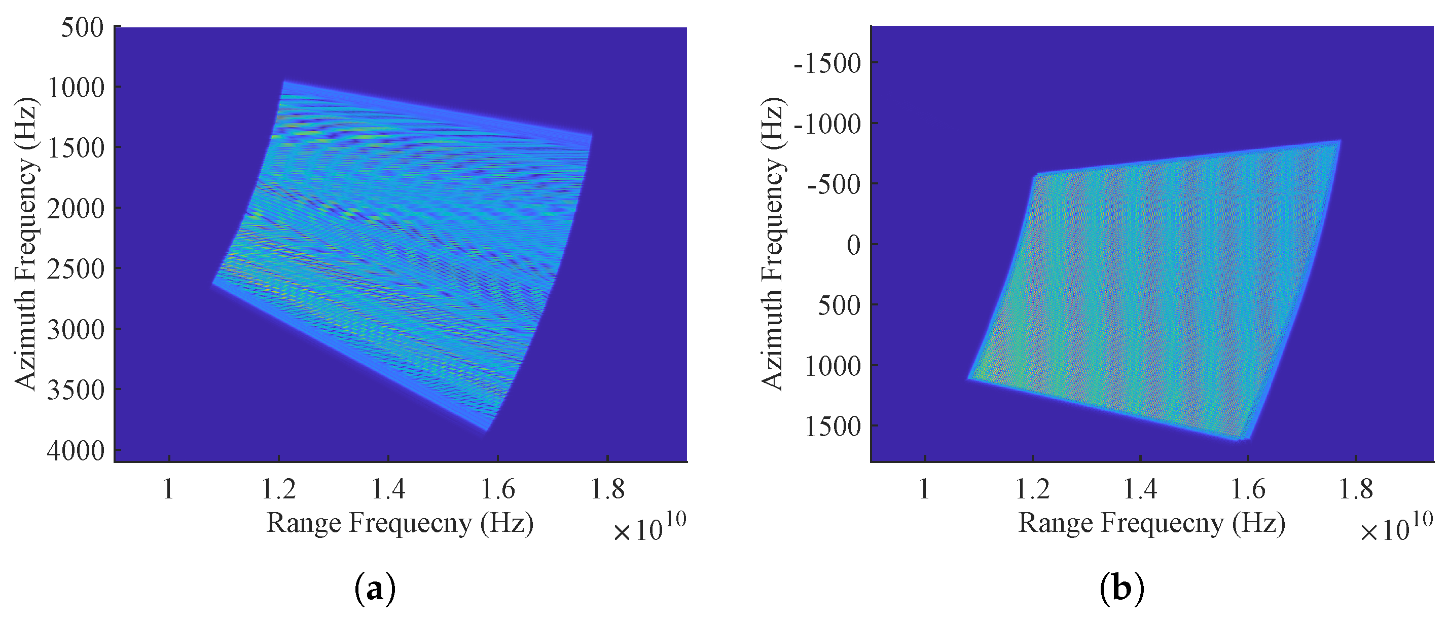
2.2.2. Azimuth Spectrum Shifting

For conventional autofocus methods, it is often assumed that the phase error is space-invariant in the azimuth time domain, while this is not the case in the azimuth-wavenumber domain [28]. Therefore, the purpose of azimuth spectrum shifting is twofold: (1) to align the azimuth wavenumber support regions, so that the phase error can be considered space-invariant in the wavenumber domain, and (2) to translate the azimuth wavenumber center to zero in order to minimize the negative effects brought by squint angles.

Considering a generic target whose azimuth coordinate is x, the center line of the azimuth wavenumber, i.e., the red dashed line $AB$ in Figure 4a, can be written as

$$K_{xc}=K_{y}tan{\theta }_c=K_y·\frac{x+rsin{\theta }_0}{rcos{\theta }_0},$$

(23)

where ${\theta }_c$ is the squint angle for this target at the synthetic aperture center.

Therefore, if we consider only the center line of the azimuth wavenumber, the azimuth spectrum shifting can be implemented in the $(x,K_y)$ domain by the following filter, which is derived by integrating (23) along the x dimension.

$$H_1\left(x,K_y\right)=exp\left(\int -K_y·\frac{x+rsin{\theta }_0}{rcos{\theta }_0}dx\right)=exp\left(-j{K}_y\frac{x^2+2rsin{\theta }_0·x}{2rcos{\theta }_0}\right)$$

(24)

After this step, the support region in the wavenumber domain of the target has changed from Figure 4a to Figure 4b, where the support region is moved near zero-Doppler; meanwhile, the azimuth-wavenumber support regions of different located targets are aligned. It should also be pointed out that since the phase of (24) is linearly dependent on $K_y$, it will cause an azimuth-variant space shift in the range dimension.

Different from the approximation used in Equation (38) in [34], which is written below,

$$K_{xc}=K_{rc}\frac{(x+rsin{\theta }_0)}{\sqrt{r^2+2rsin{\theta }_0·x+x^2}}\approx K_{rc}sin{\theta }_0+K_{rc}\frac{{cos}^2{\theta }_0}{r}x,$$

(25)

we derive the spectrum shift function (24) from the relationship between $K_x$ and $K_y$, not using $K_{rc}$ directly. Since $K_r$ has transformed into $K_y$ after Stolt mapping, it is more accurate in this way. Furthermore, the Taylor expansion approximation used in (25) is also circumvented in our derivation.

2.2.3. Range Spectrum Shifting

Considering the center line of the range wavenumber, i.e., the red dashed line, $CD$, in Figure 4a, it can be expressed as

$$K_{yc1}=\sqrt{K_{rc}^2-K_x^2}.$$

(26)

Then, after azimuth shifting, $CD$ in Figure 4a moved to $C^{\prime }{D}^{\prime }$ in Figure 4b, that is

$$K_{yc2}=\sqrt{K_{rc}^2-{\left(K_x+K_y·\frac{x+rsin{\theta }_0}{rcos{\theta }_0}\right)}^2}.$$

(27)

With (27), the difference of the center line of range wavenumber between squint and side-looking mode can be written as

$$\begin{array}{cc}\hfill \Delta K_{yc}\left(K_x\right)=& K_{yc2}-\sqrt{K_{rc}^2-K_x^2}\hfill \\ \hfill \approx & \sqrt{K_{rc}^2-{\left(K_x+K_{rc}sin{\theta }_0\right)}^2}-\sqrt{K_{rc}^2-K_x^2}\hfill \\ \hfill \approx & -sin{\theta }_0·\left(K_x+\frac{K_{rc}}{2}sin{\theta }_0\right)\hfill \end{array}.$$

(28)

Ignoring the constant term in (28), range spectrum shifting can be realized in the $(K_x,y)$ domain by

$$H_2\left(K_x,y\right)=exp\left\{j{K}_{x}sin{\theta }_0·\left(y-y_{ref}\right)\right\},$$

(29)

where $y_{ref}$ is the center coordinate along the range dimension of the observed region.

Here, only the center line of the range wavenumber is considered and the spatial variance is ignored due to the approximation used in (28). Besides, the same as the azimuth spectrum shifting, the phase of (29) is linearly dependent on $K_x$; thus, it will cause a range-variant space shift in the azimuth dimension. To minimize the space shift, $y_{ref}$ is used in (29).

In fact, the range defocus has been significantly reduced after azimuth spectrum shifting. However, at this stage the spectrum is skewed in the range dimension, as shown in Figure 4b, indicating significant variation of $K_{yc}$ at different $K_x$. The range spectrum shifting is helpful to realize the tilt correction, as shown in Figure 4c, making it more reasonable to use a unified $K_{yc}$ for the 2D phase error mapping.

2.2.4. 2D Phase-Error Mapping

The exact analytical structure of the 2D phase error for Omega-K imaging has been derived as shown in (20). Since we perform the spectrum modification in the azimuth and range dimensions, respectively, it is necessary to analyze how the structure of the 2D phase error changes after the spectrum modification.

From (24) and (29), it can be observed that the wavenumber shift of one dimension is linearly related to the other, which can be simplified as $K_x\to K_x-C_1{K}_y$ and $K_y\to K_y-C_2{K}_x$, respectively, where $C_1$ and $C_2$ are constants for a specific target.

Therefore, after azimuth spectrum shifting, (20) turns into

$${\Phi }_e^{\prime }\left(K_x,K_y\right)=K_y·\zeta \left(\frac{K_x+C_1{K}_y}{K_y}\right).$$

(30)

Then, after range spectrum shifting, (30) turns into

$$\begin{array}{cc}\hfill {\Phi }_e^{\prime \prime }\left(K_x,K_y\right)=& \left(K_y+C_2{K}_x\right)·\zeta \left(\frac{K_x+C_1\left(K_y+C_2{K}_x\right)}{K_y+C_2{K}_x}\right)\hfill \\ \hfill =& K_y\left(1+C_2\frac{K_x}{K_y}\right)\zeta \left(\frac{\left(1+C_1{C}_2\right)\frac{K_x}{K_y}+C_1}{1+C_2\frac{K_x}{K_y}}\right)\hfill \end{array},$$

(31)

which can also be simplified as

$${\Phi }_e^{\prime \prime }\left(K_x,K_y\right)=K_y·\vartheta \left(\frac{K_x}{K_y}\right).$$

(32)

Comparing (20) and (32), it can be observed that, after the spectrum manipulations, despite the specific expression of the 2D phase error changes, the form of the analytical structure remains identical. Therefore, if we perform Taylor series expansion on the 2D phase error of the modified spectrum (32) with respect to $K_y$ at $K_y=K_{yc}$, the analytical relationship between the 2D phase error ${\Phi }_e(K_x,K_y)$ and the 1D APE ${\varphi }_0\left(K_x\right)$ is still the same as Equation (34) in [28], i.e.,

$${\widehat{\Phi }}_e\left(K_x,K_y\right)=\frac{K_y}{K_{yc}}{\widehat{\varphi }}_0\left(\frac{K_{yc}}{K_y}{K}_x\right).$$

(33)

2.2.5. 2D Autofocus Processing

Based on the above analysis, we propose a new 2D autofocus method for UHR squint spotlight SAR. In addition to the spectrum modification used to mitigate the RESE and range defocus, considering the spatial variance of the motion error for UHR cases, the image-blocking technique [35] is used. Furthermore, taking into account both the estimation error and the residual range-variant error, which is ignored in the 2D autofocus, another 1D range-variant autofocus [36,37,38] is performed for each sub-image following the 2D wavenumber domain autofocus. Finally, the well-focused sub-images are stitched together to produce the final output. The entire processing flowchart of the proposed method is shown in Figure 5.

There are four main steps for the autofocus of each sub-image, as detailed below.

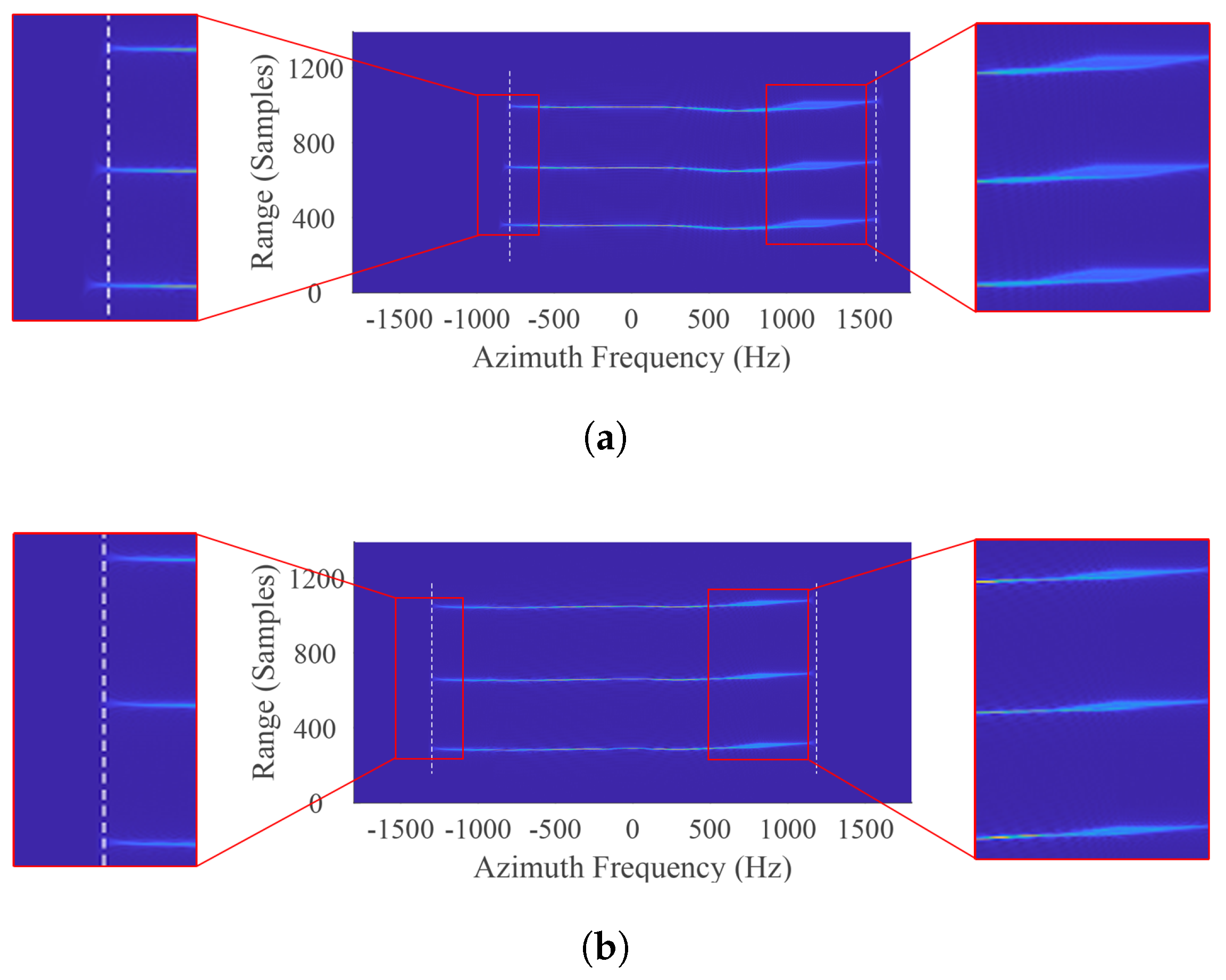
• Spectrum modification. Perform azimuth spectrum shifting with (24) in the $(x,K_y)$ domain and then range spectrum shifting with (29) in the $(K_x,y)$ domain. After that, the squint spectrum transforms into a quasi-side-looking one. The range defocus and RESE can be greatly alleviated, and the support regions of targets at different locations are aligned in the wavenumber domain.
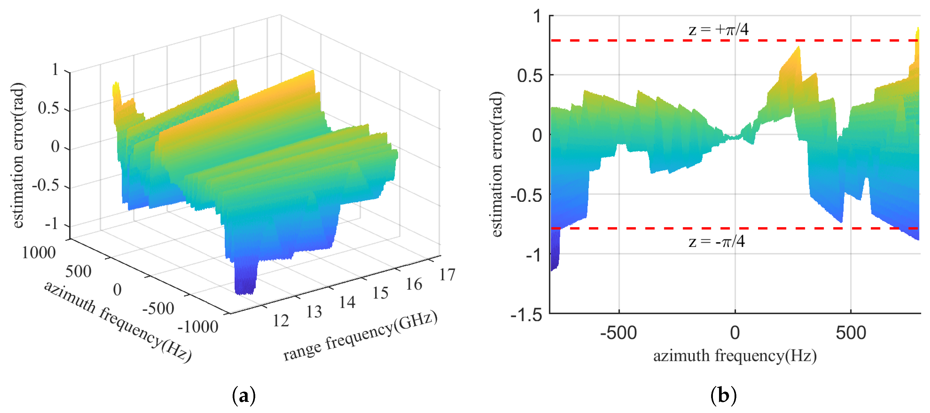
• Phase error estimation and correction. In order to obtain an accurate estimation of APE, we need first to eliminate the effect of the RESE, which can be completed by the downsampling method [27] or minimum entropy method [39]. The former enlarges the range cell by downsampling so that the RESE will be smaller than one range cell. The latter estimates the RESE by entropy minimization of the average range profile. After that, the APE can be estimated with conventional autofocus methods such as PGA [22] in the aligned range-Doppler domain. Then, with the estimated APE, perform 2D mapping using (33) and compensate for it in the 2D wavenumber domain.
• Inverse spectrum modification. This is the inverse process of step 1. Perform range and azimuth spectrum shifting with the conjugate of (29) and (24) sequentially. After this step, the support region of the spectrum is restored to its original position.
• Second 1D autofocus. Considering the estimation error and the residual range-variant RESE and APE within each block after the 2D compensation, we perform 1D range-variant autofocus on the result of step 3 with the method in [36,37,38].

3. Results

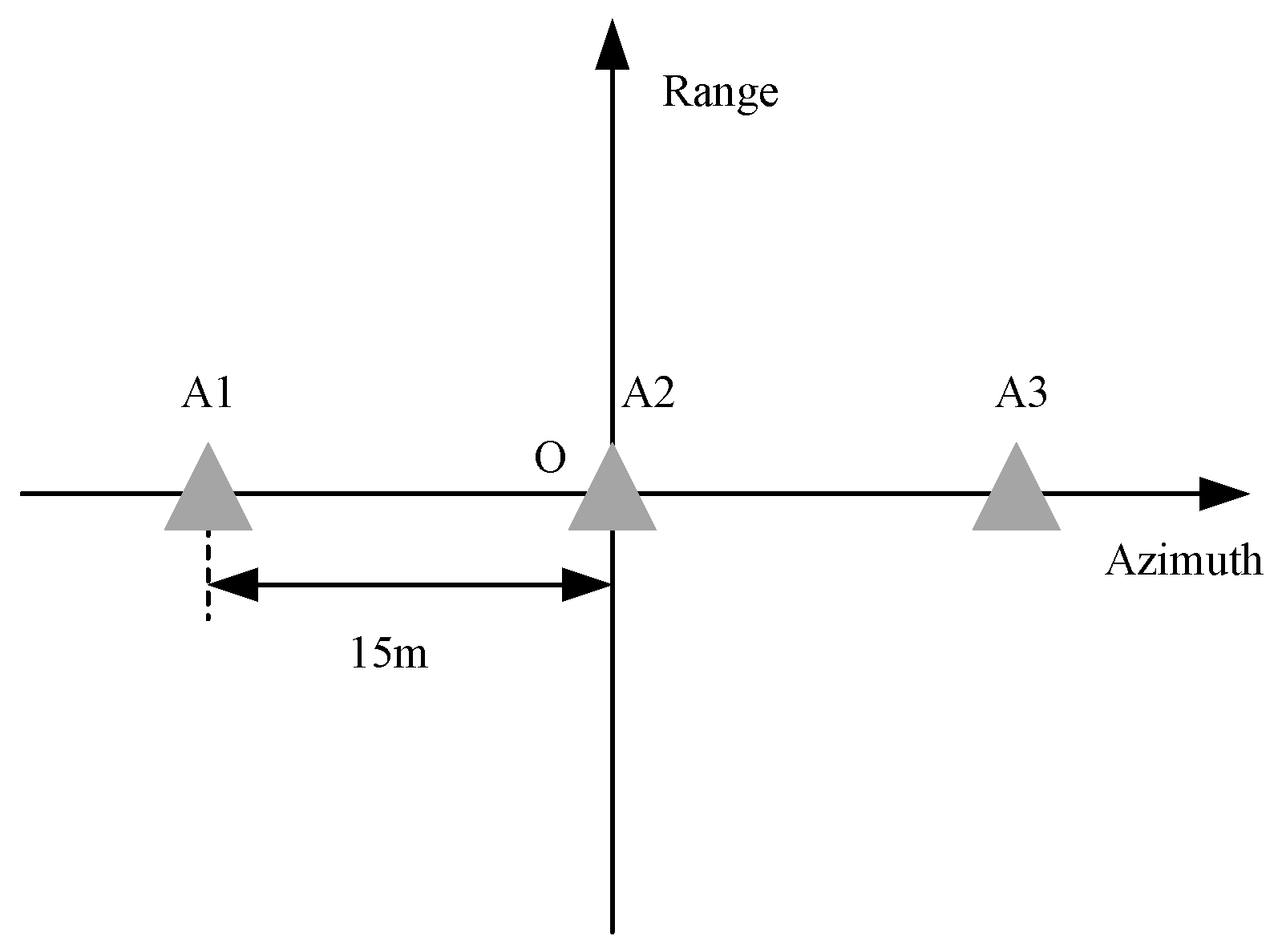
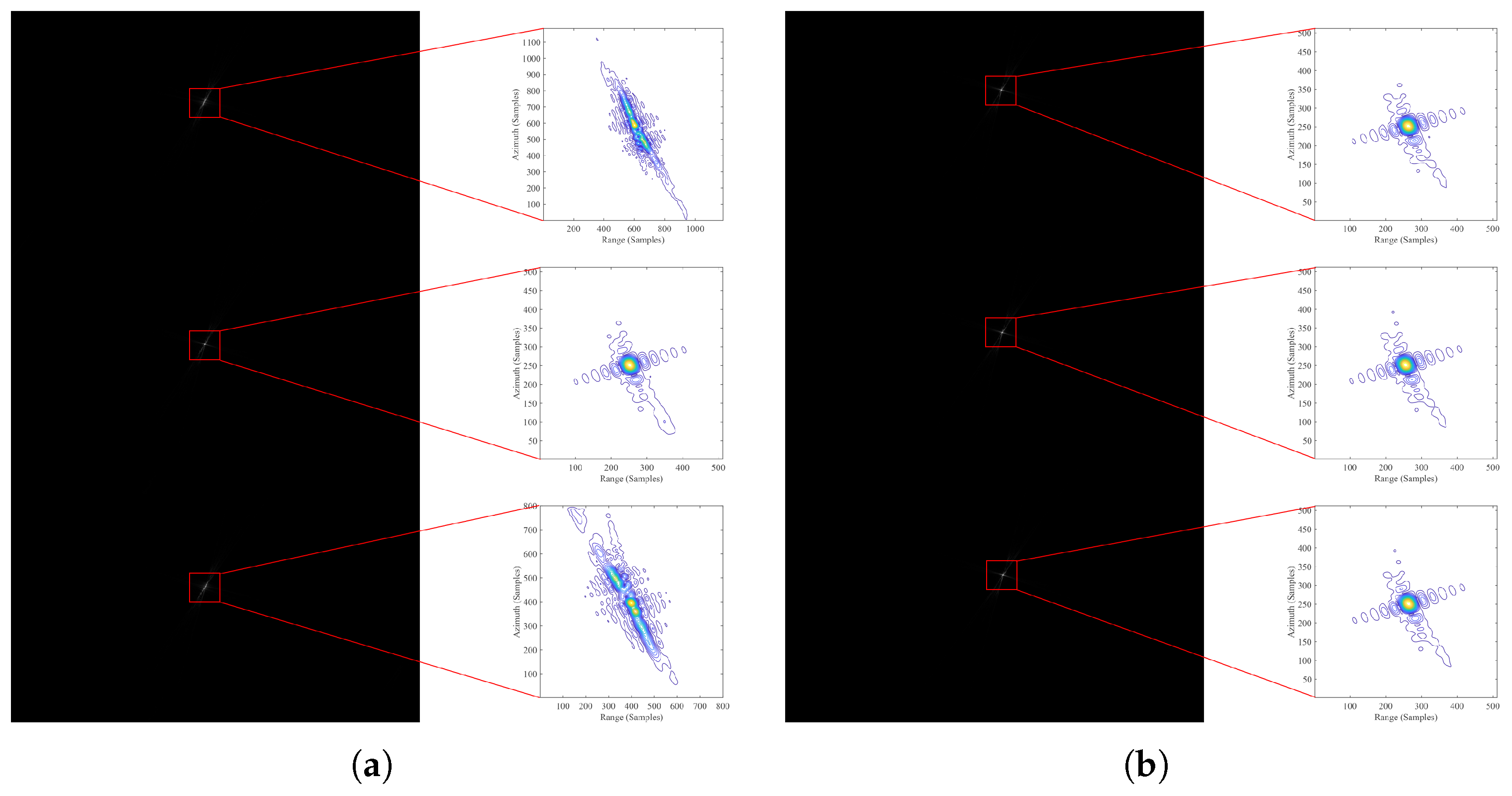
3.1. Phase Error Analysis and Performance Comparison

To analyze the phase error intuitively and show the superiority of the proposed method over the referenced method in [34], we simulate with the parameters shown in Table 2, and the squint angle is set to be ${20}^{\circ }$. The motion error is shown in Figure 2. The scene consists of three point targets distributed along the azimuth direction with adjacent intervals of 15 m, i.e., $A1$(−15 m, 0), $A2$(0, 0), and $A3$(+15 m, 0), as illustrated in Figure 6. The simulated echo data is 16,002 × 26,900 points.

3.1.1. 2D Phase Error Analysis

First, we analyze the rationality of compensating the 2D phase error of these three azimuth-distributed point targets in the wavenumber domain uniformly. The differences of the actual 2D phase error between $A1$ and $A2$, $A3$ and $A2$ after spectrum alignment are presented in Figure 7, from which we can see that the differences of the phase error are smaller than $\pi /4$; hence, it is rational to perform the phase error estimation and compensation using the middle point $A2$ as a reference.

Then, we discuss the necessity of the second 1D autofocus. We examine the estimation error of the middle target, $A2$. Figure 8a,b show the actual and the estimated phase errors of the middle target. Although they have similar shapes, the estimation error is unavoidable, which is shown in Figure 9a. For clarity, we also show the side view of Figure 9a in Figure 9b, where we can see that, at both ends of the azimuth frequency, the estimation error is greater than $\pi /4$. Despite the estimation error, we compensate the 2D phase error using the estimated one. The 2D compensated results are shown in Figure 10, where the second row of range profiles shows that the range dimension is well focused, while the third row of the azimuth dimension indicates that there is still evident phase error along the azimuth dimension. Therefore, a second 1D autofocus is necessary due to the estimation error during the 2D autofocus process, even though the range variance of the error is out of consideration in this simulation.

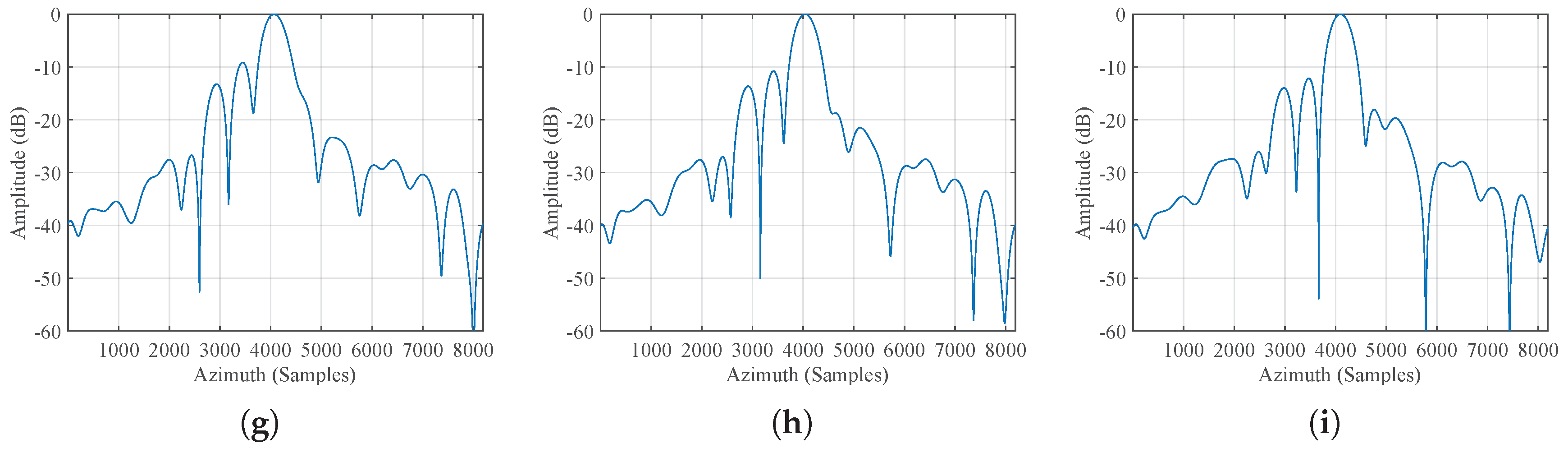
3.1.2. Performance Comparison

After analyzing the phase error in the previous part, we carry out 2D autofocus with the alignment method in [34] and the proposed method, respectively.

Figure 11 shows the variation of the 2D spectrum, where Figure 11a is the original spectrum, corresponding to the sketch in Figure 4a, Figure 11b is the spectrum after alignment with the method in [34], Figure 11c,d are the spectrum after azimuth and rang alignment with the proposed method, corresponding to the sketches in Figure 4c,d, respectively. Due to the approximation used in [34], the spectrum after processing appears to deviates from the zero-Doppler and is not fully aligned, as shown in Figure 11b. Whereas after the proposed azimuth processing, the spectrum is more aligned, as shown in Figure 11c. Furthermore, as shown in Figure 11d, our range processing eliminates any observed tilt in the range dimension.

Figure 12 shows the range envelope in the range-Doppler domain using the alignment method in [34] and the proposed method. Due to the deviation from zero-Doppler, the range defocus in Figure 12a is more severe than that in Figure 12b, as shown in the enlarged red box at the right side, which degrades the estimation accuracy. Furthermore, the compensation effect of the referenced method is also undermined by the misalignment shown in the enlarged red box at the left side of Figure 12a. Whereas the lines in Figure 12b are more aligned, which is beneficial for the subsequent estimation and correction of the phase error. For these reasons, the final result of the referenced method is worse, especially for the edge targets, as shown in Figure 13a. In comparison, the focusing performance of the proposed method is obviously better, as shown in Figure 13b. In order to provide a quantitative demonstration of the superiority of the proposed method over the referenced method in [34], we measured the entropy and contrast of the results of Figure 13, which are presented in

Table 3. Image quality index of the three azimuth-distributed point targets.

	Referenced Method	Proposed Method
Entropy	5.9719	4.4266
Contrast	13.3200	17.5166

.

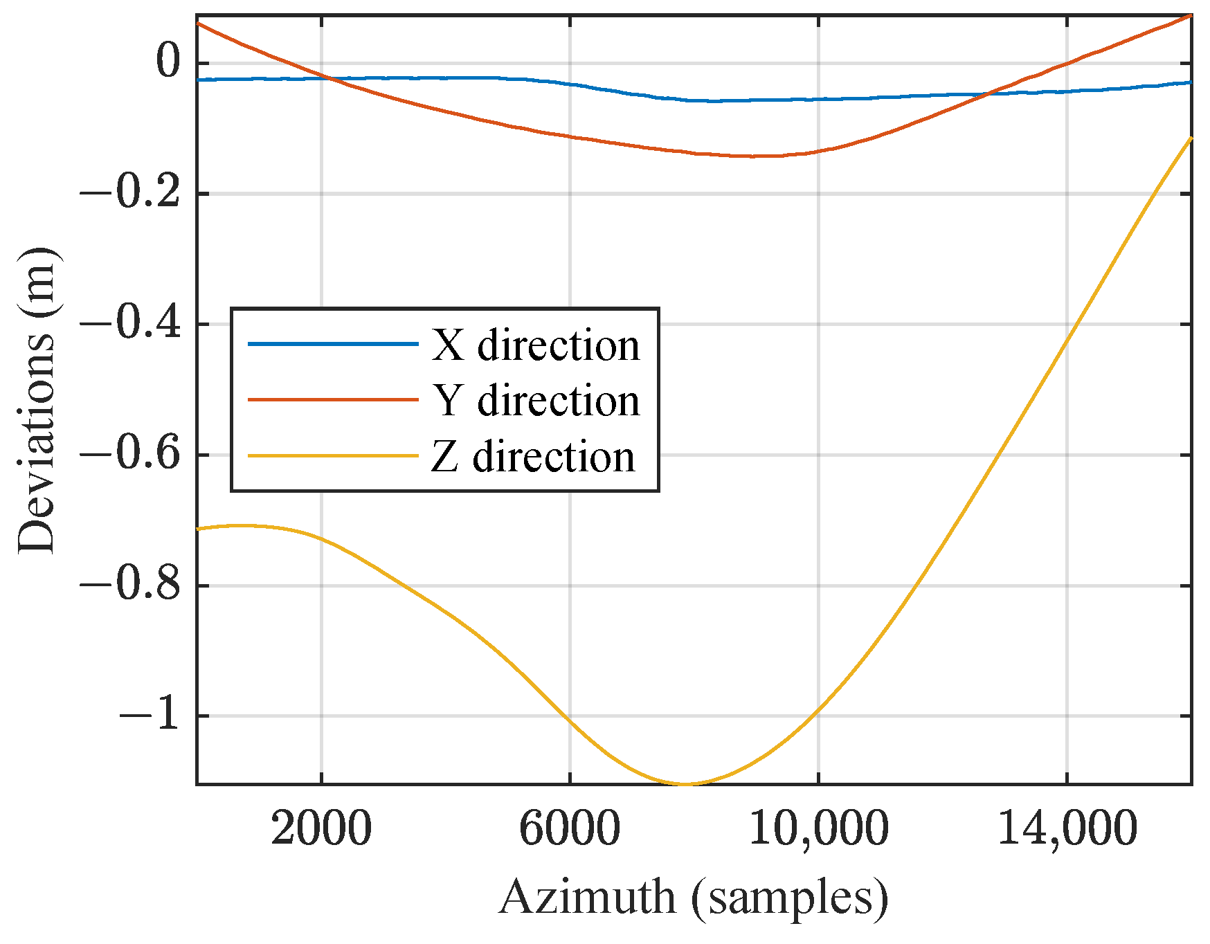
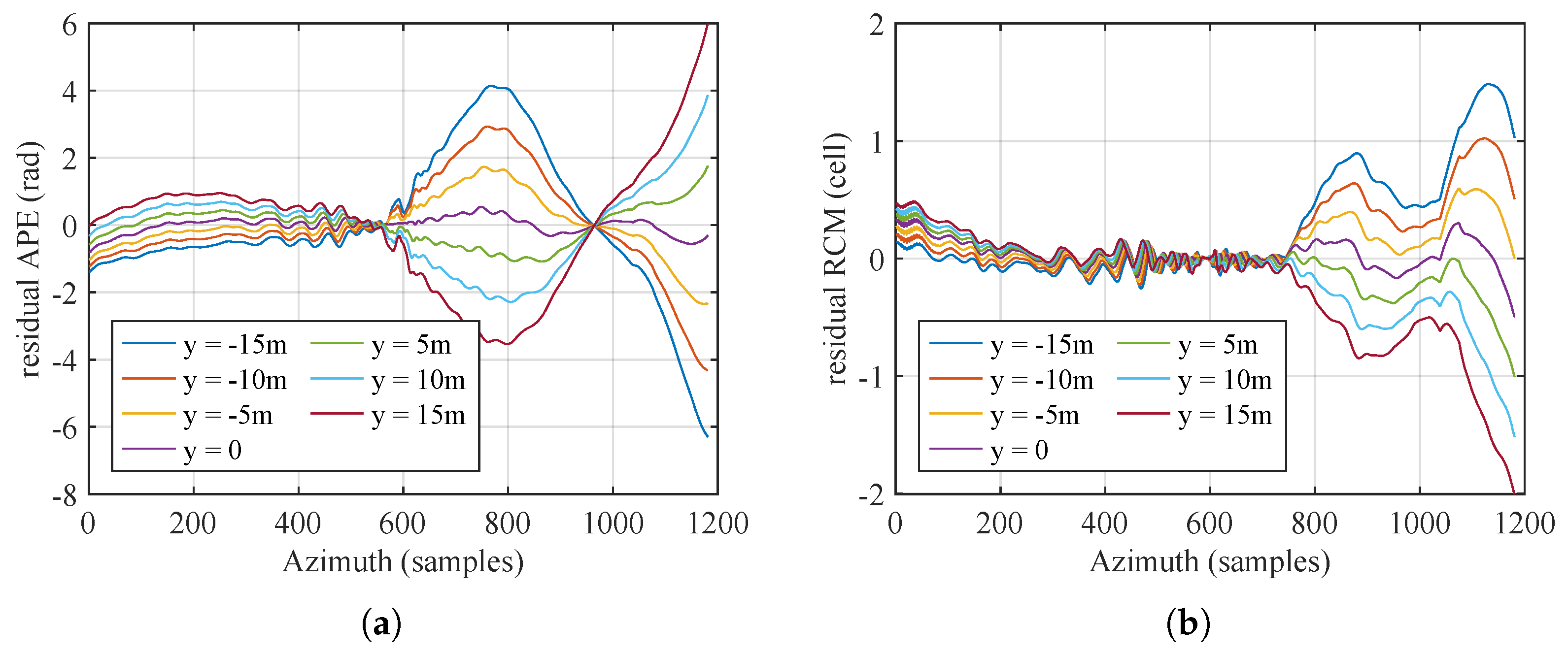
3.2. Range-Variant Compensation

In the previous section, we simulated three azimuth-distributed point targets without considering the range-variance of the phase error. In this section, we simulate seven range-distributed point targets, namely $R1$(0, −15 m), $R2$(0, −10 m), $R3$(0, −5 m), $R4(0,0)$, $R5$(0, +5 m), $R6$(0, +10 m), and $R7$(0, +15 m), as illustrated in Figure 14.

First, we perform 2D compensation using the middle target, $R4$, as a reference. The residual APE ${\varphi }_0\left(K_x\right)$ and RESE ${\varphi }_1\left(K_x\right)$ are shown in Figure 15. We can see that, after uniform 2D compensation, the maximum residual APEs of those non-reference points are greater than $\pi /4$, and the maximum residual RESEs of those non-reference points are larger than $1/2$ range cell.

To deal with such range-variant residual errors, we refer to the LS-based range-variant APE correction method [36] and the CZT-based range-variant RESE correction method [37,38]. After the estimation and correction of the range-variant RESEs and APEs by the second 1D autofocus, the residual RESEs and APEs of the seven targets at this stage are shown in Figure 16, where the residual APEs are less than $\pi /4$ and the residual RESEs are less than $1/2$ range cell, confirming the necessity and effectiveness of the range-variant envelope error and phase error compensation method adopted in the second 1D autofocus.

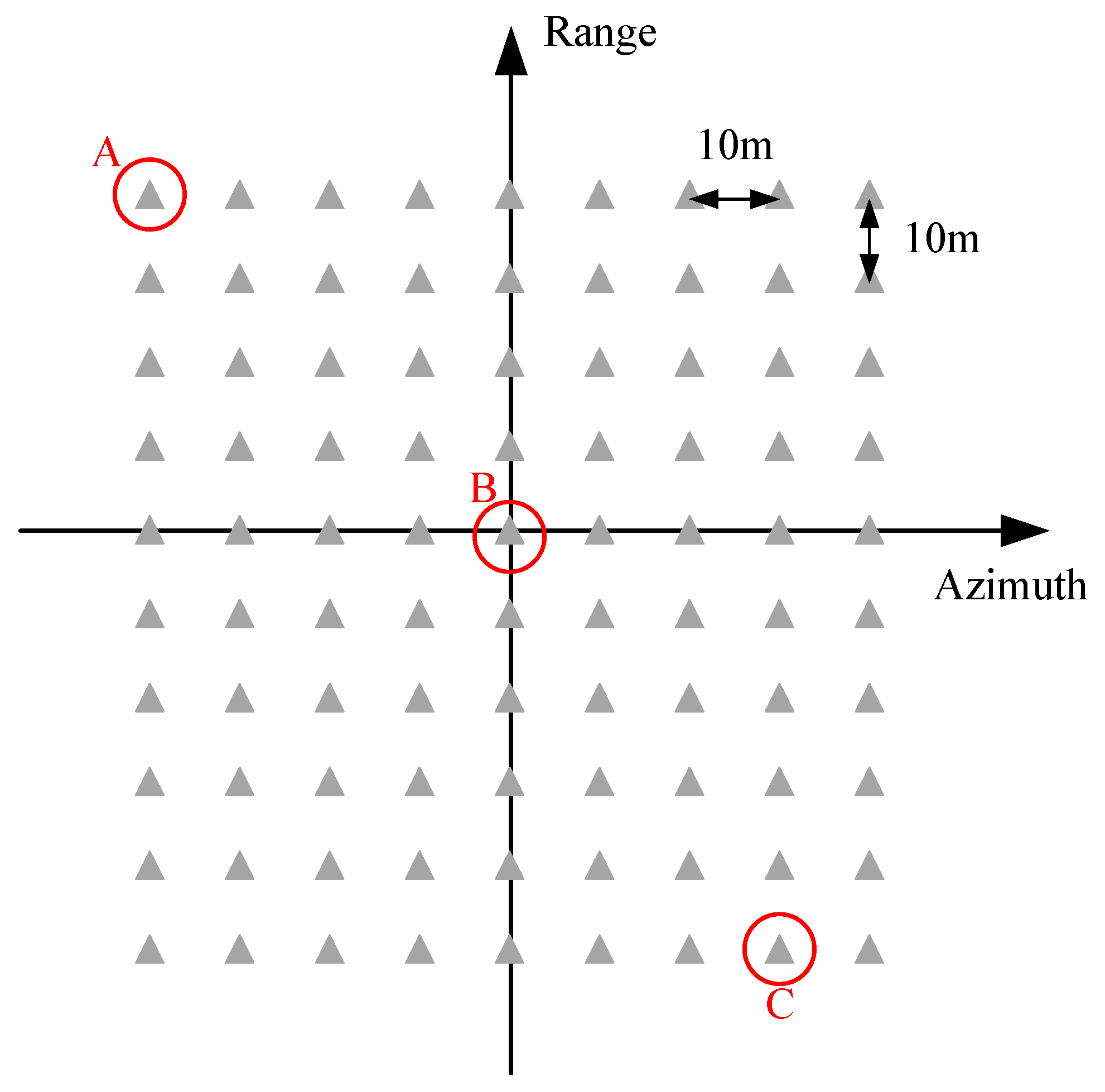
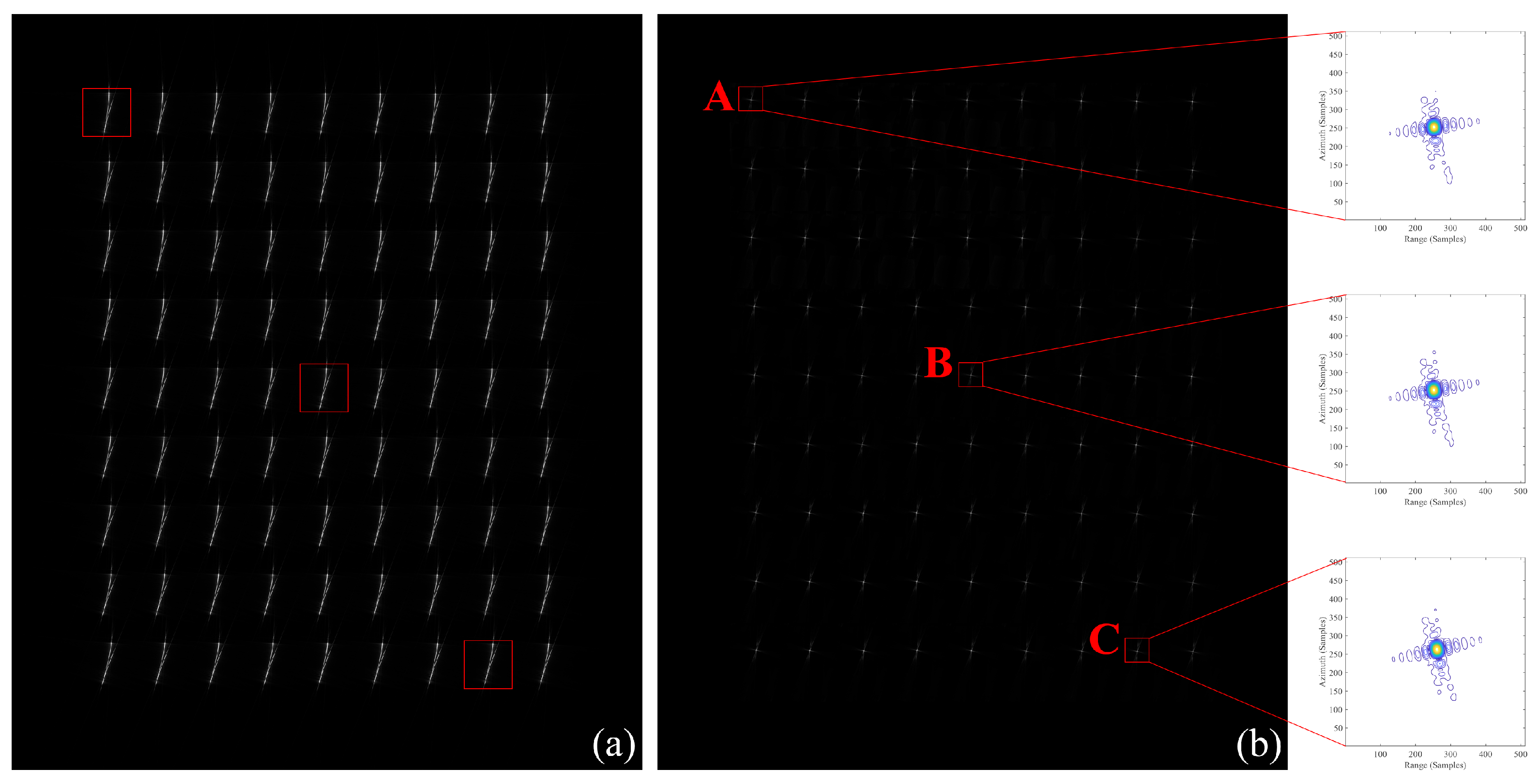
3.3. Large Scenario Verification

To further validate the effectiveness of the proposed method, we simulate with the same parameters and motion errors as shown in Table 2 and Figure 2 for a large scenario. The squint angle is set to be ${10}^{\circ }$. The scene is composed of 81 point targets evenly distributed in the $(x,y)$ direction. The interval of adjacent targets in both directions is 10 m, as illustrated in Figure 17. The simulated echo data is 16,002 × 27,200 points.

Figure 18a shows the original coarse-focused image processed by Omega-K without motion compensation. The entire image is divided into 30 m × 30 m blocks for autofocus processing. The final well-focused image is presented in Figure 18b and the enlarged contour images of the three targets indicated by red boxes are shown on the right side. The quality indexes, including impulse response width (IRW), peak sidelobe ratio (PSLR), and integral sidelobe ratio (ISLR), of the three targets are presented in

Table 4. Index measurement results of the focused targets.

	Range			Azimuth
Point	IRW (m)	PSLR (dB)	ISLR (dB)	IRW (m)	PSLR (dB)	ISLR (dB)
A	0.0236	−13.116	−10.442	0.0260	−12.535	−12.823
B	0.0238	−13.053	−10.298	0.0268	−12.420	−12.612
C	0.0239	−13.076	−10.281	0.0278	−12.358	−12.529

. The enlarged contour images and the quality indexes together confirm the significant effectiveness of the proposed method.

4. Discussion

In this article, a novel 2D autofocus method for UHR squint spotlight airborne SAR is proposed. This method addresses the problem of frequency dependence of the motion error by compensating for higher-order terms through a two-dimensional phase error mapping relationship. Additionally, it tackles the problem of spatial variance of the motion error in UHR cases by integrating the image-blocking technique and range-variant autofocus method into the processing flow.

It is challenging to effectively compensate for the frequency- and spatial-dependence of the motion error. This dilemma arises from the fact that the former requires compensation in the 2D frequency domain, while the latter necessitates compensation in the 2D image domain. It cannot be achieved simultaneously, unless point-by-point processing is employed, which entails significant computational resources. Image-blocking is a compromise between the aforementioned problem. By partitioning the entire image into small pieces, the spatial variance of the higher-order terms of the error is ignored within each sub-image. Then, the second 1D autofocus compensates for part of the range-variant errors, i.e., the constant term, ${\varphi }_0\left(K_x\right)$ and the first-order term, ${\varphi }_1\left(K_x\right)$.

To ensure that the spatial variance of the motion error can be ignored within each sub-image, the size of the image-blocking, which is determined by both the radar parameters and the magnitude of the motion errors, needs careful consideration. For a given azimuth time, $\eta$, the trajectory deviations of the radar in the Y and Z directions are represented by $\Delta y\left(\eta \right)$ and $\Delta z\left(\eta \right)$, respectively. Then, for two differently located target whose incident angle at this azimuth time are ${\gamma }_1\left(\eta \right)$ and ${\gamma }_2\left(\eta \right)$, respectively, the instantaneous slant range error for them can be calculated as follows,

$$\Delta R_i\left(\eta \right)\approx -\Delta x\left(\eta \right)·sin\left({\gamma }_i\left(\eta \right)\right)+\Delta z\left(\eta \right)·cos\left({\gamma }_i\left(\eta \right)\right)(i=1,2).$$

(34)

Then, the phase error of the two targets at $\eta$ can be expressed as

$${\varphi }_i\left(\eta \right)\approx -\frac{4\pi }{\lambda }·\Delta R_i\left(\eta \right)=-\frac{4\pi }{\lambda }·\left(-\Delta x\left(\eta \right)·sin\left({\gamma }_i\left(\eta \right)\right)+\Delta z\left(\eta \right)·cos\left({\gamma }_i\left(\eta \right)\right)\right)(i=1,2).$$

(35)

With (35), the phase error of targets at different locations can be calculated, thereby providing a reference for the selection of the size of the image-blocking. In our simulation, with the given parameters, the maximum difference of the phase error for two targets at a distance of 30 m in the azimuth is approximately 0.25 rad, smaller than $\pi /4$; thus, the phase error within a region of such a size can be considered spatially invariant.

Next, the estimation accuracy of the proposed method is discussed. In the proposed method, the APE is initially estimated, after which the APE estimation result is employed to calculate the 2D phase error. Therefore, the accuracy of the method depends on both the APE estimation accuracy and the interpolation precision during the 2D mapping. In our simulations, we use PGA for APE estimation. To enhance estimation accuracy, improved versions of PGA, such as QPGA [40] and the weighted PGA [41], can also be employed. Besides, PGA is a dominant point-based method, which implies that dominant points are required for obtaining reliable estimation results. As the number of dominant points increases, the estimation results become more accurate. Indeed, all PGA-based autofocus methods are subject to the same problem of being constrained by dominant points. If no dominant scatters exist and there are no available manually placed corner reflectors, other APE estimation algorithms, such as image-optimization-based methods, can be considered as potential alternatives.

Then, the computational complexity of the referenced method in [34] and the proposed method is analyzed and compared. The present analysis solely concerns the autofocus processing of a single sub-image. Suppose the size of one sub-image is $N_a$ and $N_r$ points in the azimuth and range dimensions, respectively, and the interpolation kernel length used for 2D phase error mapping is L. The referenced method comprises three range FFTs/IFFTs, two azimuth FFTs/IFFTs, three phase multiplications, $N_r$ times azimuth interpolation, and one APE estimation. Since APE estimation is identical for the two methods, we use $C_{APE}$ to represent the computational complexity for it, which is dependent on the selected estimation algorithm and the iteration times. Thus, the computational complexity of the reference method can be calculated as

$$\begin{array}{cc}\hfill C_1& =3\times 5N_a{N}_{r}lo{g}_2{N}_r+2\times 5N_a{N}_{r}lo{g}_2{N}_a+3\times 6N_a{N}_r+2(2L-1)N_a{N}_r+C_{APE}\hfill \\ \hfill & =N_a{N}_r\left(15lo{g}_2{N}_r+10lo{g}_2{N}_a+16+4L\right)+C_{APE}\hfill \end{array}.$$

(36)

The proposed method contains six range FFTs/IFFTs, two azimuth FFTs/IFFTs, five phase multiplications, $N_r$ times azimuth interpolation, and one APE estimation, which is calculated as

$$\begin{array}{cc}\hfill C_2& =6\times 5N_a{N}_{r}lo{g}_2{N}_r+2\times 5N_a{N}_{r}lo{g}_2{N}_a+5\times 6N_a{N}_r+2(2L-1)N_a{N}_r+C_{APE}\hfill \\ \hfill & =N_a{N}_r\left(30lo{g}_2{N}_r+10lo{g}_2{N}_a+28+4L\right)+C_{APE}\hfill \end{array}.$$

(37)

Compared with the referenced method, the proposed method has an additional pair of range spectrum shifting operations in the range time-azimuth-frequency domain, thus adding the number of transitions between range time-frequency domains and the phase multiplication times. Nevertheless, a slight increase in computational complexity can be anticipated, which is tolerable in order to achieve enhanced focusing capabilities.

For UHR radar with centimeter resolution, several systems based on microwave photonic (MWP) technology have been built in recent years [42]. The simulation parameters we used in this paper are set according to a real MWP SAR system published in [3]. However, the available measured airborne UHR SAR data are all in broadside mode [3,4,43]. Since the MWP SAR is still in the development stage, the airborne MWP SAR data is scarce and the squint data is not yet available. Although subaperture data can be used to equate the echoes acquired with a squint angle, the azimuth resolution will decrease accordingly, which is not desired for our purpose. Consequently, we present only experiments on simulated data in this paper.

In addition, for UHR airborne SAR systems, the gyro-stabilized sensor is employed to effectively isolate carrier disturbances and maintain platform stability. For instance, the gyro-stabilized sensor mount ‘Leica PAV80’ exhibits a nominal root mean square error of ${0.02}^{\circ }$, which can be ignored during SAR data processing. Therefore, in this paper, we do not consider the squint angle error caused by the attitude variations. Besides, the cases of highly nonlinear flight tracks are not within the scope of this paper.

5. Conclusions

This article proposes a new 2D wavenumber domain autofocus method for UHR squint spotlight airborne SAR based on an improved spectrum modification strategy. Compared to the existing methods, this approach considers the dependence of range defocus on the squint angle and employs an improved spectrum modification strategy, which can transform the spectrum of squint mode into a quasi-side-looking one, and meanwhile achieve alignment in azimuth and tilt correction in range. After that, the compensation in the wavenumber domain is completed with the 2D phase error mapping. Furthermore, to account for the spatial-variant motion error, the proposed method incorporates image-blocking and range-dependent motion error compensation methods. The effectiveness of the proposed method is verified by simulations. Future research will focus on the extension of the proposed method to stripmap mode.

References

1. Carrara, W.G.; Goodman, R.S.; Majewski, R.M. Spotlight Synthetic Aperture Radar: Signal Processing Algorithms; Artech House: Norwood, MA, USA, 1995. [Google Scholar]
2. Cumming, I.G.; Wong, F.H. Digital Signal Processing of Synthetic Aperture Radar Data: Algorithms and Implementation; Artech House: Norwood, MA, USA, 2004. [Google Scholar]
3. Li, R.; Li, W.; Dong, Y.; Wen, Z.; Zhang, H.; Sun, W.; Yang, J.; Zeng, H.; Deng, Y.; Luan, Y.; et al. PFDIR—A Wideband Photonic-Assisted SAR System. IEEE Trans. Aerosp. Electron. Syst. 2023, 59, 4333–4346. [Google Scholar] [CrossRef]
4. Deng, Y.; Xing, M.; Sun, G.C.; Liu, W.; Li, R.; Wang, Y. A Processing Framework for Airborne Microwave Photonic SAR With Resolution Up To 0.03 m: Motion Estimation and Compensation. IEEE Trans. Geosci. Remote Sens. 2022, 60, 1–17. [Google Scholar] [CrossRef]
5. Chen, M.; Qiu, X.; Li, R.; Li, W.; Fu, K. Analysis and Compensation for Systematical Errors in Airborne Microwave Photonic SAR Imaging by 2D Autofocus. IEEE J. Sel. Topics Appl. Earth Observ. Remote Sens. 2023, 16, 2221–2236. [Google Scholar] [CrossRef]
6. Guo, Y.; Wang, P.; Zhou, X.; He, T.; Chen, J. A Decoupled Chirp Scaling Algorithm for High-Squint SAR Data Imaging. IEEE Trans. Geosci. Remote Sens. 2023, 61, 1–17. [Google Scholar] [CrossRef]
7. Chen, X.; Hou, Z.; Dong, Z.; He, Z. Performance Analysis of Wavenumber Domain Algorithms for Highly Squinted SAR. IEEE J. Sel. Topics Appl. Earth Observ. Remote Sens. 2023, 16, 1563–1575. [Google Scholar] [CrossRef]
8. Chen, J.; Xing, M.; Yu, H.; Liang, B.; Peng, J.; Sun, G.C. Motion Compensation/Autofocus in Airborne Synthetic Aperture Radar: A Review. IEEE Geosci. Remote Sens. Mag. 2022, 10, 185–206. [Google Scholar] [CrossRef]
9. Jin, M.Y.; Wu, C. A SAR correlation algorithm which accommodates large-range migration. IEEE Trans. Geosci. Remote Sens. 1984, GE-22, 592–597. [Google Scholar] [CrossRef]
10. Raney, R.K.; Runge, H.; Bamler, R.; Cumming, I.G.; Wong, F.H. Precision SAR processing using chirp scaling. IEEE Trans. Geosci. Remote Sens. 1994, 32, 786–799. [Google Scholar] [CrossRef]
11. Wong, F.H.; Cumming, I.G. Error Sensitivities of a Secondary Range Compression Algorithm for Processing Squinted Satellite Sar Data. In Proceedings of the IGARSS, Vancouver, BC, Canada, 10–14 July 1989; Volume 4, pp. 2584–2587. [Google Scholar] [CrossRef]
12. Moreira, A.; Huang, Y. Airborne SAR processing of highly squinted data using a chirp scaling approach with integrated motion compensation. IEEE Trans. Geosci. Remote Sens. 1994, 32, 1029–1040. [Google Scholar] [CrossRef]
13. Davidson, G.W.; Cumming, I.G.; Ito, M.R. A chirp scaling approach for processing squint mode SAR data. IEEE Trans. Aerosp. Electron. Syst. 1996, 32, 121–133. [Google Scholar] [CrossRef]
14. An, D.; Huang, X.; Jin, T.; Zhou, Z. Extended Nonlinear Chirp Scaling Algorithm for High-Resolution Highly Squint SAR Data Focusing. IEEE Trans. Geosci. Remote Sens. 2012, 50, 3595–3609. [Google Scholar] [CrossRef]
15. Sun, G.; Xing, M.; Liu, Y.; Sun, L.; Bao, Z.; Wu, Y. Extended NCS Based on Method of Series Reversion for Imaging of Highly Squinted SAR. IEEE Geosci. Remote Sens. Lett. 2011, 8, 446–450. [Google Scholar] [CrossRef]
16. Munson, D.; O’Brien, J.; Jenkins, W. A tomographic formulation of spotlight-mode synthetic aperture radar. Proc. IEEE 1983, 71, 917–925. [Google Scholar] [CrossRef]
17. Cafforio, C.; Prati, C.; Rocca, F. SAR data focusing using seismic migration techniques. IEEE Trans. Aerosp. Electron. Syst. 1991, 27, 194–207. [Google Scholar] [CrossRef]
18. Samczynski, P.; Kulpa, K.S. Coherent MapDrift Technique. IEEE Trans. Geosci. Remote Sens. 2010, 48, 1505–1517. [Google Scholar] [CrossRef]
19. Zhang, L.; Hu, M.; Wang, G.; Wang, H. Range-Dependent Map-Drift Algorithm for Focusing UAV SAR Imagery. IEEE Geosci. Remote Sens. Lett. 2016, 13, 1158–1162. [Google Scholar] [CrossRef]
20. Wang, J.; Liu, X. SAR Minimum-Entropy Autofocus Using an Adaptive-Order Polynomial Model. IEEE Geosci. Remote Sens. Lett. 2006, 3, 512–516. [Google Scholar] [CrossRef]
21. Gao, Y.; Yu, W.; Liu, Y.; Wang, R.; Shi, C. Sharpness-Based Autofocusing for Stripmap SAR Using an Adaptive-Order Polynomial Model. IEEE Geosci. Remote Sens. Lett. 2014, 11, 1086–1090. [Google Scholar] [CrossRef]
22. Wahl, D.E.; Eichel, P.H.; Ghiglia, D.C.; Jakowatz, C.V. Phase gradient autofocus-a robust tool for high resolution SAR phase correction. IEEE Trans. Aerosp. Electron. Syst. 1994, 30, 827–835. [Google Scholar] [CrossRef]
23. Van Rossum, W.L.; Otten, M.P.G.; Van Bree, R.J.P. Extended PGA for range migration algorithms. IEEE Trans. Aerosp. Electron. Syst. 2006, 42, 478–488. [Google Scholar] [CrossRef]
24. Zhu, D.; Jiang, R.; Mao, X.; Zhu, Z. Multi-Subaperture PGA for SAR Autofocusing. IEEE Trans. Aerosp. Electron. Syst. 2013, 49, 468–488. [Google Scholar] [CrossRef]
25. Zeng, T.; Wang, R.; Li, F. SAR Image Autofocus Utilizing Minimum-Entropy Criterion. IEEE Geosci. Remote Sens. Lett. 2013, 10, 1552–1556. [Google Scholar] [CrossRef]
26. Morrison, R.L.; Do, M.N.; Munson, D.C. SAR Image Autofocus By Sharpness Optimization: A Theoretical Study. IEEE Trans. Image Process. 2007, 16, 2309–2321. [Google Scholar] [CrossRef]
27. Doerry, A.W. Autofocus Correction of Excessive Migration in Synthetic Aperture Radar Images; Technical Report; Sandia National Laboratories (SNL): Albuquerque, NM, USA; Livermore, CA, USA, 2004.
28. Mao, X.; He, X.; Li, D. Knowledge-Aided 2D Autofocus for Spotlight SAR Range Migration Algorithm Imagery. IEEE Trans. Geosci. Remote Sens. 2018, 56, 5458–5470. [Google Scholar] [CrossRef]
29. Mao, X.; Zhu, D. Two-dimensional Autofocus for Spotlight SAR Polar Format Imagery. IEEE Trans. Comput. Imag. 2016, 2, 524–539. [Google Scholar] [CrossRef]
30. Mao, X.; Ding, L.; Zhang, Y.; Zhan, R.; Li, S. Knowledge-Aided 2-D Autofocus for Spotlight SAR Filtered Backprojection Imagery. IEEE Trans. Geosci. Remote Sens. 2019, 57, 9041–9058. [Google Scholar] [CrossRef]
31. Zhang, L.; Sheng, J.; Xing, M.; Qiao, Z.; Xiong, T.; Bao, Z. Wavenumber-Domain Autofocusing for Highly Squinted UAV SAR Imagery. IEEE Sens. J. 2012, 12, 1574–1588. [Google Scholar] [CrossRef]
32. Xu, G.; Xing, M.; Zhang, L.; Bao, Z. Robust Autofocusing Approach for Highly Squinted SAR Imagery Using the Extended Wavenumber Algorithm. IEEE Trans. Geosci. Remote Sens. 2013, 51, 5031–5046. [Google Scholar] [CrossRef]
33. Ran, L.; Liu, Z.; Li, T.; Xie, R.; Zhang, L. Extension of Map-Drift Algorithm for Highly Squinted SAR Autofocus. IEEE J. Sel. Topics Appl. Earth Observ. Remote Sens. 2017, 10, 4032–4044. [Google Scholar] [CrossRef]
34. Lin, H.; Chen, J.; Xing, M.; Chen, X.; You, D.; Sun, G. 2-D Frequency Autofocus for Squint Spotlight SAR Imaging With Extended Omega-K. IEEE Trans. Geosci. Remote Sens. 2022, 60, 1–12. [Google Scholar] [CrossRef]
35. Zhang, L.; Wang, G.; Qiao, Z.; Wang, H.; Sun, L. Two-Stage Focusing Algorithm for Highly Squinted Synthetic Aperture Radar Imaging. IEEE Trans. Geosci. Remote Sens. 2017, 55, 5547–5562. [Google Scholar] [CrossRef]
36. Chen, J.; Liang, B.; Zhang, J.; Yang, D.G.; Deng, Y.; Xing, M. Efficiency and Robustness Improvement of Airborne SAR Motion Compensation With High Resolution and Wide Swath. IEEE Geosci. Remote Sens. Lett. 2022, 19, 1–5. [Google Scholar] [CrossRef]
37. Chen, J.; Liang, B.; Yang, D.G.; Zhao, D.J.; Xing, M.; Sun, G.C. Two-Step Accuracy Improvement of Motion Compensation for Airborne SAR With Ultrahigh Resolution and Wide Swath. IEEE Trans. Geosci. Remote Sens. 2019, 57, 7148–7160. [Google Scholar] [CrossRef]
38. Chen, J.; Xing, M.; Sun, G.C.; Li, Z. A 2-D Space-Variant Motion Estimation and Compensation Method for Ultrahigh-Resolution Airborne Stepped-Frequency SAR With Long Integration Time. IEEE Trans. Geosci. Remote Sens. 2017, 55, 6390–6401. [Google Scholar] [CrossRef]
39. Zhu, D.; Wang, L.; Yu, Y.; Tao, Q.; Zhu, Z. Robust ISAR Range Alignment via Minimizing the Entropy of the Average Range Profile. IEEE Geosci. Remote Sens. Lett. 2009, 6, 204–208. [Google Scholar] [CrossRef]
40. Chan, H.L.; Yeo, T.S. Noniterative quality phase-gradient autofocus (QPGA) algorithm for spotlight SAR imagery. IEEE Trans. Geosci. Remote Sens. 1998, 36, 1531–1539. [Google Scholar] [CrossRef]
41. de Macedo, K.A.C.; Scheiber, R.; Moreira, A. An Autofocus Approach for Residual Motion Errors With Application to Airborne Repeat-Pass SAR Interferometry. IEEE Trans. Geosci. Remote Sens. 2008, 46, 3151–3162. [Google Scholar] [CrossRef]
42. Panda, S.S.S.; Panigrahi, T.; Parne, S.R.; Sabat, S.L.; Cenkeramaddi, L.R. Recent Advances and Future Directions of Microwave Photonic Radars: A Review. IEEE Sens. J. 2021, 21, 21144–21158. [Google Scholar] [CrossRef]
43. Li, R.; Li, W.; Dong, Y.; Wang, B.; Wen, Z.; Luan, Y.; Yang, Z.; Yang, X.; Yang, J.; Sun, W.; et al. An Ultrahigh-Resolution Continuous Wave Synthetic Aperture Radar with Photonic-Assisted Signal Generation and Dechirp Processing. In Proceedings of the 2020 17th European Radar Conference (EuRAD), Utrecht, The Netherlands, 10–15 January 2021; pp. 13–16. [Google Scholar] [CrossRef]
Figure 1. Geometric model of squint SAR.
Remotesensing 16 02158 g001
Figure 2. Trajectory deviation of the radar platform.
Remotesensing 16 02158 g002
Figure 3. Range envelopes in range-Doppler domain for different squint angles. (a) 0 , (b) 10 , (c) 20 and (d) 30 .
Remotesensing 16 02158 g003
Figure 4. The variations of the spectrum support region. (a) The original support region of a target whose squint angle at the synthetic aperture center is θ c . (b) The support region after azimuth spectrum shifting. (c) The support region after range spectrum shifting.
Remotesensing 16 02158 g004
Figure 5. Flowchart of the proposed 2D autofocus method. The variations of the 2D spectrum of three point targets during processing are shown on both sides.
Remotesensing 16 02158 g005
Figure 6. Three azimuth-distributed point targets with adjacent intervals of 15 m.
Remotesensing 16 02158 g006
Figure 7. The differences of the actual 2D phase error between (a) the targets A 1 and A 2 , (b) the targets A 3 and A 2 .
Remotesensing 16 02158 g007
Figure 8. (a) The actual and (b) estimated 2D phase error of the middle target, A 2 .
Remotesensing 16 02158 g008
Figure 9. (a) Estimation error of the middle target, A 2 . (b) Side view of (a).
Remotesensing 16 02158 g009
Figure 10. (ac) are the enlarged contour images of the three azimuth-distributed point targets after 2D phase error correction. (df) are the range profiles corresponding to (ac). (gi) are the azimuth profiles corresponding to (ac).
Remotesensing 16 02158 g010aRemotesensing 16 02158 g010b
Figure 11. 2D Spectrum. (a) Before processing. (b) After processing with the method in [34]. (c) After azimuth processing of the proposed method. (d) After range processing of the proposed method.
Remotesensing 16 02158 g011aRemotesensing 16 02158 g011b
Figure 12. Range-Doppler domain of the image after azimuth spectrum shifting by (a) the method in [34] and (b) the proposed method.
Remotesensing 16 02158 g012
Figure 13. Processing results and enlarged contour images of three azimuth-distributed point targets with (a) the alignment method in [34] and (b) the proposed method. The sizes of (a,b) are both 2364 × 1392 pixels.
Remotesensing 16 02158 g013
Figure 14. Seven range-distributed point targets with adjacent intervals of 5 m.
Remotesensing 16 02158 g014
Figure 15. (a) The residual APE ϕ 0 ( K x ) and (b) RESE ϕ 1 ( K x ) of the seven range-distributed point targets after 2D compensation.
Remotesensing 16 02158 g015
Figure 16. (a) The residual APE ϕ 0 ( K x ) and (b) RESE ϕ 1 ( K x ) of the seven range-distributed point targets after range-variant 1D autofocus.
Remotesensing 16 02158 g016
Figure 17. Eighty-one point targets evenly distributed in the ( x , y ) direction with adjacent intervals of 10 m in both directions.
Remotesensing 16 02158 g017
Figure 18. (a) The original image of a large scenario processed by Omega-K. (b) Stitched fine-focused result processed by the proposed method. The sizes of (a,b) are both 5910 × 4924 pixels.
Remotesensing 16 02158 g018