Article

Validation of Gross Primary Production Estimated by Remote Sensing for the Ecosystems of Doñana National Park through Improvements in Light Use Efficiency Estimation

by
Pedro J. Gómez-Giráldez
1,*,
Jordi Cristóbal
2,
Héctor Nieto
3,
Diego García-Díaz
1 and
Ricardo Díaz-Delgado
1
1
Estación Biológica de Doñana (EBD-CSIC), C/Americo Vespucio, s/n, 41092 Sevilla, Spain
2
Departament de Geografía, Universitat Autònoma de Barcelona, Campus de Bellaterra, Edifici B, Carrer de la Fortuna, s/n, 08193 Bellaterra, Spain
3
Instituto de Ciencias Agrarias (ICA-CSIC), C/Serrano 115 bis, 28006 Madrid, Spain
*
Author to whom correspondence should be addressed.
Remote Sens. 2024, 16(12), 2170; https://doi.org/10.3390/rs16122170
Submission received: 5 April 2024 / Revised: 5 June 2024 / Accepted: 13 June 2024 / Published: 15 June 2024
(This article belongs to the Special Issue Remote Sensing Application in the Carbon Flux Modelling)

Abstract

:
Doñana National Park is located in the southwest of the Iberian Peninsula, where water scarcity is recurrent, together with a high heterogeneity in species and ecosystems. Monitoring carbon assimilation is essential to improve knowledge of global change in natural vegetation cover. In this work, a light use efficiency (LUE) model was applied to estimate gross primary production (GPP) in two ecosystems of Doñana, xeric shrub (drought resistant) and seasonal marsh (with grasslands dependent on water hydroperiod) and validated with in situ data from eddy covariance (EC) towers installed in both ecosystems. The model was applied in two ways: (1) using the fraction of absorbed photosynthetically active radiation (FAPAR) from Sentinel-2 and meteorological data from reanalysis (ERA5), and (2) using Sentinel-2 FAPAR, reanalysis solar radiation (ERA5) and the Sentinel-2 land surface water index (LSWI). In both cases and for both ecosystems, the error values are acceptable (below 1 gC/m2) and in both ecosystems the model using the LSWI gave better results (R2 of 0.8 in marshes and 0.51 in xeric shrubs). The results also show a greater influence of the water status of the system than of the meteorological variables in this area.

1. Introduction

The Doñana National Park (DNP), located in the southwestern part of the Iberian Peninsula, is one of the most important wetlands in Europe and is home to a great diversity of ecosystems and species. It is estimated that more than 300 species of birds, 1300 species of vascular plants, and 27 species of continental fish live in Doñana [1].
The ecosystems of Doñana play a key role in the carbon cycle, storing and releasing large amounts of CO2 through photosynthesis and respiration [2]. Within the animal community, in addition to wild ungulates, there are native breeds of domestic livestock in an extensive regime, such as the “retuerta” horse and the “mostrenca” cow, which graze in these ecosystems, and thus accounting for carbon assimilation allows us to know the availability of forage. This scenario makes carbon assimilation in Doñana a very relevant parameter to monitor.
Carbon assimilation is essential for understanding the underlying mechanisms of the global carbon cycle [3] and is defined as a derived metric to study and manage biodiversity change [4,5]. However, climate change is affecting plant functioning and altering plant carbon fluxes, with a decrease in carbon assimilation that is particularly pronounced in Mediterranean ecosystems such as the southwestern part of the Iberian Peninsula [6,7,8].
A commonly used indicator of carbon assimilation is gross primary production (GPP) [9,10], which is the rate of carbon fixation per unit time and over a defined area [11,12,13]. In general, methods for measuring GPP and CO2 fluxes have mostly been developed and evaluated for arable land (e.g., [14,15,16]). Therefore, the application of these methods in natural vegetation is the next challenge. This is particularly important in Mediterranean ecosystems, where vegetation represents different layers, low vegetation cover and many different species and plant functional types. Flux towers or eddy covariance (EC) towers provide the necessary measurements to estimate surface energy and carbon fluxes in natural land cover and to calibrate and evaluate land surface models [17,18]. However, an EC only covers an area (footprint) that varies with the tower height, target surface properties, and the wind direction and speed [19]. For regional scale assessment, it is necessary to combine it with other data sources such as Earth observation imagery to estimate GPP at both spatial and temporal scales [20,21]. There are several remote sensing-based models for estimating GPP, which can be broadly classified into four types: (1) statistical models, (2) light use efficiency (LUE) models, (3) process models integrated with RS parameters, and (4) machine learning approaches [22]. Recently, LUE models have experienced rapid development [23] and have been successfully applied to estimate GPP in different ecosystems and climates using different sources of remote sensing imagery (e.g., [24,25,26]). However, there are few studies on carbon assimilation by remote sensing in the Doñana ecosystems (e.g., [27,28,29]), and these are mostly focused on the Doñana marshes. Furthermore, there are no estimates for sparse xeric scrub, which are needed to improve our knowledge of the role of sparsely vegetated areas in carbon assimilation [30].
LUE models are based on the work of Monteith [31,32] and assume that GPP is proportional to the product of the absorbed photosynthetically active radiation (APAR) by vegetation and the efficiency with which this radiation is converted into biomass. APAR is usually calculated as the product of FAPAR and incoming photosynthetically active radiation (PAR), which can be operatively derived from satellite data [33,34]. LUE depends on environmental and physiological factors that may limit photosynthesis, such as temperature, humidity, water stress, or nutrition. This means that there are several ways to approach GPP estimation, with LUE applications focusing more on meteorological variables [35] and others using water stress indices [36].
The objective of this paper is to analyze two parameterizations for LUE to estimate the GPP with Sentinel-2 imagery in two different ecosystems in the Doñana protected area: (i) marshes, which are seasonal wetlands flooded in winter, and (ii) xeric Mediterranean scrub adapted to drought, using the LUE model. Two LUE model approaches will be applied, depending on how the light use efficiency is parameterized: (i) using meteorological data, and (ii) focusing on water availability. The results will be evaluated with data collected by two flux towers (eddy covariance, EC) installed by the Singular Scientific and Technological Infrastructure of the Doñana Biological Reserve (ICTS-DBR) in both ecosystems from 2020 to 2022 for the xeric Mediterranean scrub, and 2021–2022 for the Doñana marsh.

2. Materials and Methods

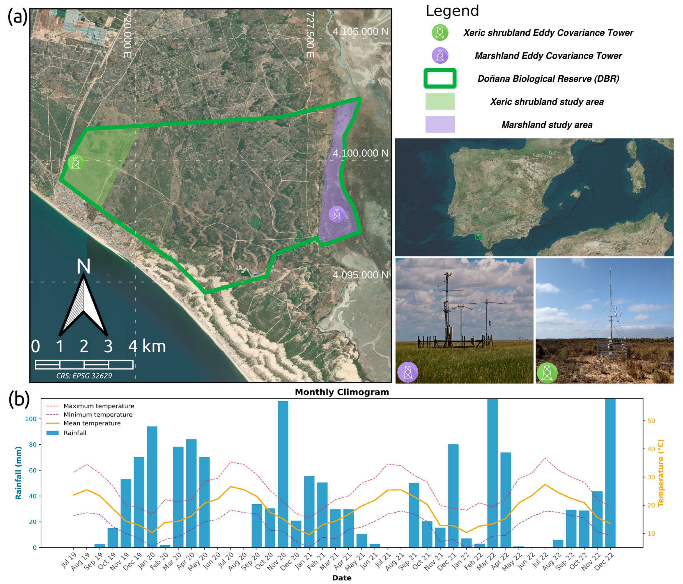
2.1. Study Site, Instrumentation and Data Sources

The DNP, covering 53,700 ha, is a UNESCO Biosphere Reserve and Natural Heritage and a Ramsar Site, located in the southwest of the Iberian Peninsula. It includes the Doñana Biological Reserve (DBR) of 6109 ha (Figure 1a), a core conservation area where ICTS-DBR has established a scientific infrastructure providing long-term monitoring data and access to the scientific community. Figure 1b shows the climogram of the area on a monthly scale. It shows the accumulated precipitation as well as the averages of maximum, minimum and mean temperatures. The average annual precipitation is 548.6 mm and the average annual temperature is 18.4 °C, based on data from the DBR meteorological stations. However, there is a large interannual and seasonal variability in precipitation and temperature, which affects the hydrological and ecological dynamics of the Doñana ecosystems. Different ecosystems are represented in the DBR, such as lagoons, dunes, marshes, shrub areas or forest areas of pine, juniper, or cork oak. The morphology of the area defines two distinct soil zones: sand (littoral and aeolian systems) and mud-clay (estuarine system) [37]. Our study focuses on two Doñana ecosystems: xeric Mediterranean scrub on sandy soils and seasonal marsh on mud-clay soils (Figure 1a), two ecosystems with opposite water dependencies but close enough to be exposed to the same climatic conditions. In this study, similar time frames were chosen depending on the availability of EC data, from July 2019 to December 2022 for xeric shrublands and from October 2020 to December 2022 for marshes.
The xeric Mediterranean scrub is a semi-arid ecosystem, which represents about 629 ha of the DBR, dominated by xeric shrubs such as Rosmarinus officinalis, Halymium halymifolium, and Halymium commutatum, growing on sandy soils with low organic matter and with functional traits for drought [38,39]. The Doñana marsh is a seasonal wetland that is flooded in winter by rainfall and tributaries, forming an extensive floodplain (537.78 ha in the DBR), mainly dominated by the helophytes Bolboschoenus maritimus, Schoenoplectus lacustris, Juncus subulatus and Arthrocnemum macrostachyum, and the macrophytes Ranunculus peltatus, Rupia drepanensis, Chara galiodes and Myriohpyllum alterniflorum.
In both ecosystems, the ICTS-DBR installed an EC system (Figure 1a) with a height of 4.75 m for the xeric shrubland (latitude: 37.020206, longitude: −6.554403) and 3.9 m for the swamp (latitude: 36.998539, longitude: −6.434575). The sensors and variables used in this study are listed in Table 1.
The remote sensing products used, along with their source, spatial resolution, and number of images, are summarized in Table 2. The products used for this study are described in detail in the following sections.

2.2. LUE Model

An adaptation of the LUE model, which relates incident solar radiation to the photosynthetic activity of vegetation according to Equation (1) [31,32], was used.
GPP = FAPAR × PAR × ε
where GPP (gC/m2) is the gross primary production, FAPAR (dimensionless) is the fraction of photosynthetically active radiation absorbed by the plant, PAR (MJ/m2) is the photosynthetically active radiation, and ε (gC/MJ) is the light use efficiency parameter. FAPAR and PAR were estimated in the same way for both xeric shrubland and swamp ecosystems, while two different methods were used for ε (see sections below).

2.2.1. FAPAR Estimation

A time series of 257 FAPAR scenes was selected from the high-resolution vegetation phenology and productivity product of the Copernicus Land Monitoring Service (CMLS) (https://land.copernicus.eu/en/products/vegetation (accessed on 13 January 2023)) with a spatial resolution of 10 m and a temporal resolution of 5 days. This product uses a 6S radiative transfer model in the canopy methodology implemented in the SNAP Toolbox (SNAP—ESA Sentinel Application Platform v2.0.2, http://step.esa.int (accessed on 12 January 2023)) to estimate FAPAR at 20 m spatial resolution. The methodology of [40] is then applied to obtain a final product at 10 m spatial resolution [41]. This methodology was implemented to generate biophysical products such as leaf area, index, FAPAR and fractional vegetation cover from multiple sensors. It consists mainly in generating a comprehensive database of vegetation characteristics and associated Sentinel 2 top of canopy (TOC) reflectances. Later, neural networks are trained to estimate the canopy characteristics from the TOC reflectances along with defined corresponding angles that determine the observation configuration. For the massive download of all images for the entire study period and their subsequent clipping to the DBR area, a Python package was created (https://pypi.org/project/pyvpp (accessed on 19 October 2023)). Finally, the resulting images were linearly interpolated pixel by pixel to produce a daily image.

2.2.2. PAR Estimation

The PAR estimate is based on the daily incoming shortwave radiation data using a conversion factor from shortwave (400–2500 nm) to PAR (400–700 nm) of 0.48. This coefficient was determined by [42] from measurements at several points around the globe. The daily incoming shortwave radiation data were obtained from the ERA5 land reanalysis at a spatial resolution of 11,132 m and were produced by replaying the land component of the ECMWF ERA5 climate reanalysis [43]. A total of 1278 daily aggregated periods corresponding to the surface_solar_radiation_downwards_sum dataset were extracted using the Google Earth Engine platform [44].

2.2.3. ε Estimation

The estimation of ε is based on the determination of a maximum ε value (εmax), which is reduced by environmental parameters/conditions. The value of εmax (gC/MJ) is specific to each land cover and even to each species [45], with variations also depending on the geographical area. In this case, a value of 3 g/MJ was used for xeric shrublands, which is similar to the values for woody cover in semi-arid zones [46,47], and a value of 2 g/MJ was used for swamps, since the dominant species can be an intermediate value between grasslands [48] and annual crops [49].
To reduce εmax to these maximum values at both sites, two approaches were applied using meteorological variables and a water stress index.

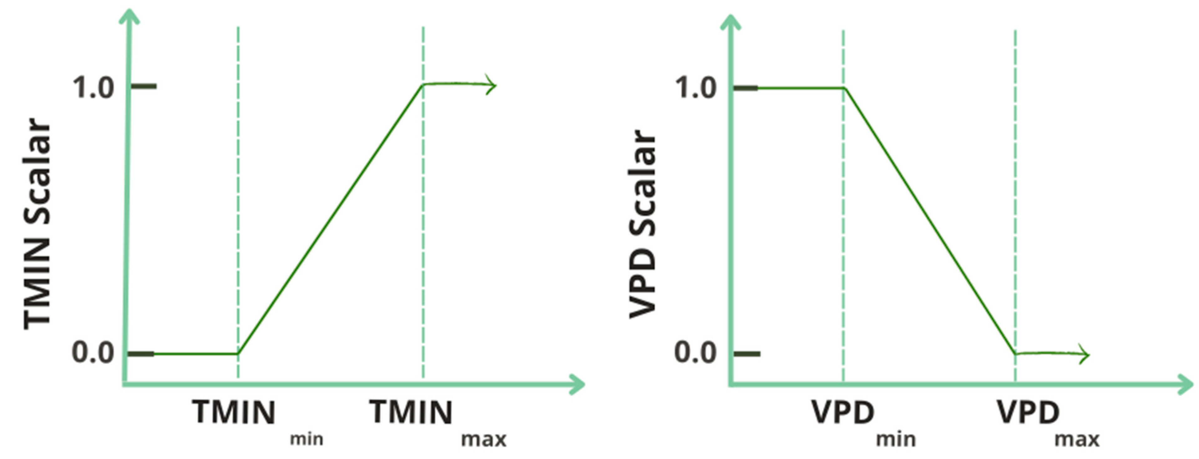
ε Reduction with Meteorological Variables

The value for εmax is modified according to the meteorological variables that reduce the efficiency of the system, the daily minimum air temperature (Tmin), and the vapor pressure deficit (VPD) according to Equation (2) [50].
ε = εmax × Tmin_sc × VPD_sc
where ε is the light use efficiency parameter, εmax is its maximum value defined in the previous section, and Tmin_sc and VPD_sc (dimensionless) are simple linear functions between 0 and 1 derived from the daily values of Tmin and VPD (Figure 2). These linear functions are obtained using threshold values, where the minimum and maximum values for Tmin are 0 and 1 of the scalar Tmin (increasing function), respectively; and the minimum and maximum values for VPD correspond to 1 and 0 of the scalar VPD (decreasing function), respectively.
Upper and lower thresholds for both variables were taken from the Biome-Property-Look-Up-Table (BPLUT) [50], using open shrubland cover (−8 and 8.8 °C for Tmin; and 0.65 and 4.8 kPa for VPD) for xeric shrubland and grassland cover (−8 and 12.02 °C for Tmin; and 0.65 and 5.3 kPa for VPD) for marshland.
Tmin was obtained from the ERA5-Land, 1278 daily aggregated arrays corresponding to the temperature_2m_min dataset.
VPD was obtained using Equation (3).
VPD = (es − a)
where VPD is the vapor pressure deficit (kPa), es is the saturated vapor pressure (kPa) obtained from Equation (4), while ea is the actual vapor pressure (kPa) obtained from Equation (5):
es = (0.611 × exp ((17.27 × Tmed)/(237.3 + Tmed)))
where Tmed is the mean air temperature (°C) obtained from the ERA5-Land, 1278 daily aggregated arrays corresponding to the temperature_2m dataset.
ea = es × RH
where RH is the relative humidity (%) obtained from Equation (6):
RH = exp((17.269 × Td)/(273.3 + Td) − (17.269 × Tmed)/(237.3 + Tmed))
where Td is the dew point temperature (K) obtained from the ERA5-Land, 1278 daily aggregated arrays corresponding to the dewpoint_temperature_2m dataset.

ε Reduction with a Water Index

For this reduction, the Land Surface Water Index (LSWI) [51] (Equation (3)) was used as a water availability index. This dimensionless index was previously applied to evaluate moisture content in vegetation as well as to evaluate soils associated with humidity in semi-arid ecosystems [52]. It is computed using Sentinel-2 bands B8 (near infrared, NIR: 835.1 nm for S2A, 833 nm for S2B) and B12 (shortwave infrared 2, SWIR2: 2202.4 nm for S2A, 2185.7 nm for S2B) according to Equation (7).
LSWI = (B8 − B12)/(B8 + B12)
where B8 and B12 are NIR and SWIR2 bands from Sentinel-2.
This index was calculated for 150 granules of Sentinel-2 images, corresponding to all available images in the study area with less than 15% of cloud coverage for the whole study period of the atmospherically corrected bottom of the atmosphere product (Level 2A) available from the European Space Agency. LSWI was resampled to 10 m and extracted in the DBR area using Google Earth Engine. The resulting images were linearly interpolated pixel by pixel in order to obtain a daily image.
Once a daily image of LSWI was obtained, the index was standardized to values between 0 and 1 to obtain a scalar LSWI (LSWI_sc) using Equation (8), similar to [53], and it was used to estimate the final value of ε using Equation (9).
LSWI_sc = (1 + LSWI)/2
where LSWI_sc is the scalar land surface water index and LSWI is the land surface water index.
ε = εmax × LSWI_sc
where ε (gC/MJ) is the light use efficiency parameter, εmax (gC/MJ) is its maximum value defined in Section 2.2.3. above and LSWI_sc is the scalar land surface water index.

2.3. Evaluation Procedure

The EC towers installed in both ecosystems were used to evaluate the model. High-frequency data (10 Hz in Table 1) were processed using the express mode of the EddyPro software (version 7.0.9 LI-COR, Lincoln, NE, USA) to generate 30-min averaged measurements of net ecosystem exchange (NEE), sensible heat (H), and latent heat (LE). The processing included several steps: correction for anemometer tilt according to [54]; despiking, which involved identifying and removing short-term outliers in the time series, often caused by electronic spikes during precipitation; identifying periods of low signal variation relative to the instrumental resolution, common in weak winds and stable conditions; and detecting relatively short periods where the time series remained constant, indicating potential problems [55]. To calculate the GPP, the measured NEE had to be partitioned. A diurnal flux partitioning algorithm [56] was used in this study through the R language package REddyproc [57]. Friction velocity (u*) filtering during periods of low turbulent mixing was also used: the minimum value was estimated according to Papale et al. (2006) [58] and applied to detect NEE saturation with increasing u* [59]. Finally, in REddyProc, a gap filling of the eddy covariance and meteorological data is performed with methods similar to Falge et al. (2005) [60], taking into account the co-variation of the fluxes with meteorological variables and the temporal autocorrelation of the fluxes, as described by Reichstein et al. (2005) [61]. Finally, the EC footprint was estimated according to Hsieh et al. (2000) [62], with the crosswind extension of Detto et al. (2006) [63], to evaluate the 2D contribution of each point in the ground to the turbulent fluxes recorded by the EC system. The footprint calculation was performed using a Python package (https://github.com/hectornieto/footprint-analysis (accessed on 24 May 2024)).
In order to compare the GPP data of the EC towers with the images resulting from the LUE models, the daily GPP and footprint data were obtained from the 30-min data. The daily footprint was resampled to the resolution of the images (10 m).
The 10 m resolution daily footprints were applied to the LUE model images, and then the EC and model data were compared using the coefficient of determination (R2) of the linear regressions to indicate the precision of the estimates relative to the observations, the root mean squared error (RMSE) and the normalized root mean squared error (NRMSE) to measure error differences, and the mean bias error (MBE) to indicate cumulative offsets between measured and observed values. These metrics were applied at both daily and monthly scales.
Finally, to obtain a spatial visualization of the results, the LUE model that yielded the best result was spatially applied, with a spatial resolution of 10 m for both ecosystems for each hydrological year (which ranges from October 1 to September 3 of the following year in the study area [64]). The terrestrial vegetation map of Doñana [65] was used to delineate these ecosystems.

3. Results

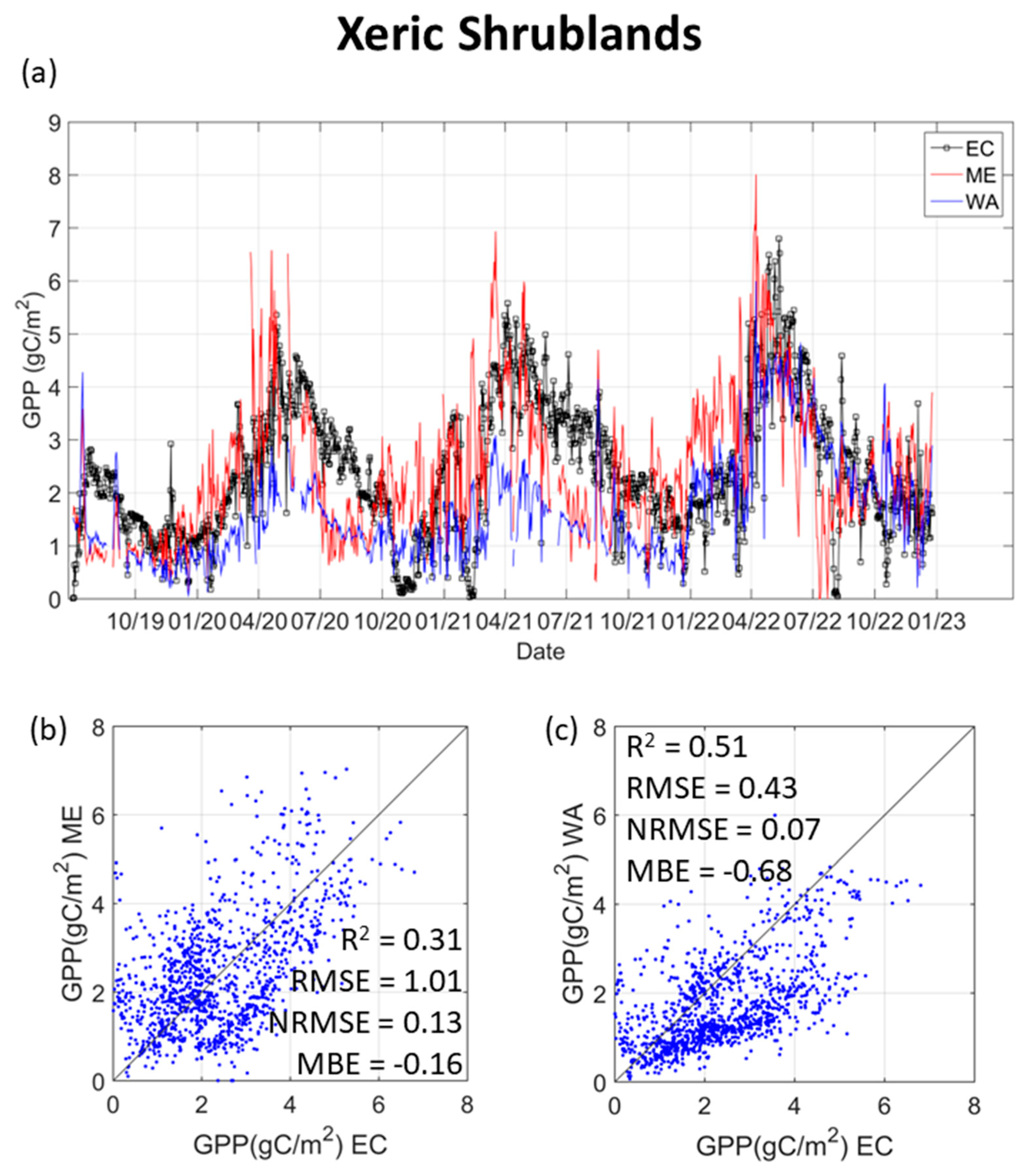
3.1. Xeric Shrubland
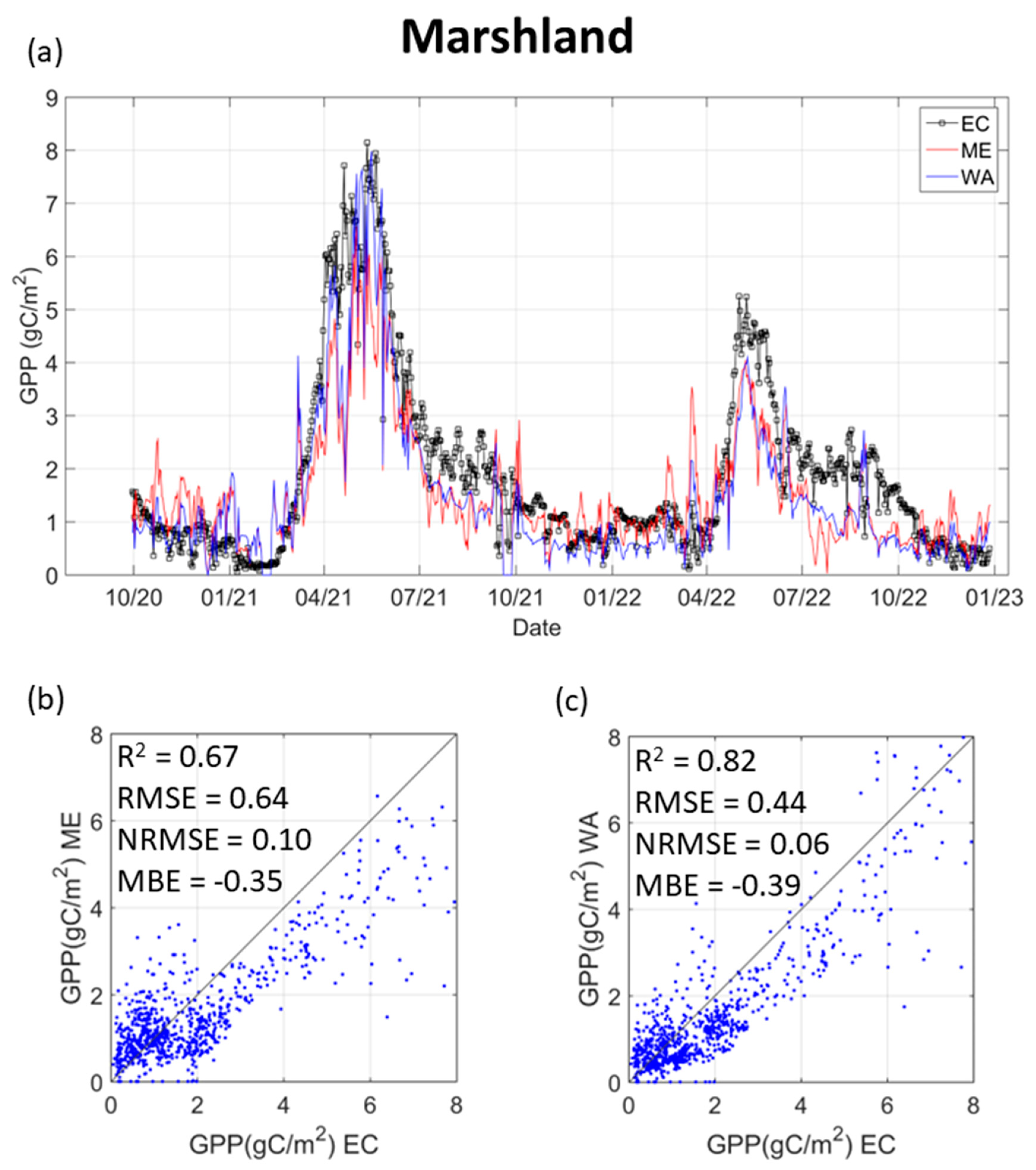
Figure 3a shows the temporal dynamics of the GPP in this ecosystem, obtained from the eddy covariance system and from the LUE models for the period from July 2019 to December 2022 at the daily scale. Cyclical behavior can be observed, with the maximum values occurring at the end of spring and the minimum at the beginning of fall, which is well reflected in the LUE models, although both show an advance in the maximum values. Regarding the interannual behavior, there is a general increase in GPP, ranging from a maximum of about 5 gC/m2days−1 in 2020 to 7 gC/m2days−1 in 2022.
The values given by the LUE model using meteorological data from ERA5-Land (hereafter ME) showed a similar but noisier trend, while the values given by the LUE model using a water availability index (hereafter WA) showed a general underestimation in the first two years studied (2019–2021), but a better fit in 2022.
These trends are evident in Figure 3b,c, which show the 1:1 plots of both models with respect to the EC data throughout the study period, together with R2, RMSE, NRMSE and MBE. ME showed more scattered values resulting in R2 of 0.31, RMSE of 1.01 gC/m2 and NRMSE of 0.13. On the other hand, the WA gave a better fit (R2 = 0.51) and lower error (RMSE = 0.43 gC/m2 and NRMSE = 0.07) despite the underestimation mentioned above. This underestimation of the WA resulted in a higher bias, with relatively high MBE values (−0.68 gC/m2) compared to those of ME (−0.16 gC/m2).
When the results were aggregated on a monthly basis (Table 3), there was an improvement in both LUE models, showing better R2 and RMSE, especially in WA, where the RMSE drops to only 0.21 gC/m2 and the R2 reaches 0.74, while the MBE and NRMSE remain constant.
Finally, using the LUE model that gave the best results, WA, the annual GPP accumulated by hydrological year in the xeric shrubland zone of the DBR, is presented in Figure 4. Several differences can be observed, from the firebreak area (redder values) without assimilation to the denser shrub areas (blue). It should be noted that although the maximum values in GPP increase, especially in 2021/2022, in the EC validation zone, at the spatial level it does not show this trend.

3.2. Marshland

The temporal dynamics of GPP in the marshland ecosystem for the period between October 2020 and December 2022 at the daily scale are shown in Figure 5a, both for the EC data and for those obtained by both LUE models. In this ecosystem, a more pronounced cycle is observed than in the case of xeric shrublands, more like a grassland ecosystem, with maximum values at the end of spring and almost zero at the beginning of winter. In the period analyzed, a significant decrease in the maximum values of carbon assimilation was observed, from about 8 g/m2 in 2021 to 5 g/m2 in 2022. In this case, both LUE models slightly underestimate, which is more noticeable at the end of summer and beginning of fall.
Both LUE models slightly underestimate, with this more pronounced in late summer and early fall (Figure 5). Despite this underestimation, both LUE models produce better results for marshlands than for xeric shrublands (shown in the 1:1 plots and their errors in Figure 5b,c). R2 is high for both approaches, although better in WA (0.82 and 0.67 for WA and ME, respectively). RMSE and NRMSE showed a similar pattern, but with lower values for WA, 0.43 gC/m2 and 0.06 compared to 0.64 gC/m2 and 0.1 for ME. Finally, the MBE showed similar values, consistent with the slight underestimation (−0.35 gC/m2 for ME and −0.39 gC/m2 for WA).
Table 4 shows the results using the monthly aggregates. The results improve in both LUE models when using monthly averages, much more clearly than in xeric shrublands, lowering the RMSE values and reaching very high R2 values, reaching up to 0.93 in the case of WA. The MBE and NRMSE remain constant with similar values compared to the daily scale.
Figure 6 shows the annual accumulated GPP using the LUE-WA model. In this case, a decrease in carbon assimilation from the hydrological year 2020/2021 to 2021/2022 can be seen very clearly.

4. Discussion

4.1. GPP Dynamics

The study of the xeric shrubland and marsh ecosystems within the DBR provides valuable insights into the dynamics of these environments and provides an example of the variability of this natural reserve. In both ecosystems, cyclical behavior was observed, with peaks centered at the end of spring, which is common in Mediterranean environments [66]. However, in the case of the xeric shrublands (Figure 3a), the decrease from maximum to minimum values is more gradual and extends over a longer period than in the marshes (Figure 5a). In fact, higher than expected values were observed in this ecosystem, being 2–3 gC/m2 higher than those of the 500 m spatial resolution product of MODIS (MOD17A2HGF) or those of other similar ecosystems [67,68]. This is because xeric shrublands are adapted to drought conditions, while swamps are not, which is also reflected in the slight increase in GPP during the study period in xeric shrublands, while there was a strong decrease in swamps, The study area is experiencing a long and intense drought, particularly dramatic in the last two hydrological years (2020/2021 and 2021/2022), with total annual precipitation below 400 mm (Figure 1b), which also negatively affects the marshland due to the faster response of the herbaceous species present in this ecosystem [69].

4.2. LUE—Models Validation

The correct application of LUE models is limited by several factors, such as uncertainty in the input data, since they are derived from remote sensing, or by the specific implementation of the model itself [70]. Both application areas have been considered sufficiently large and homogeneous for the proper use of remote sensing. However, the spatial heterogeneity of the xeric shrublands in terms of cover and different species, as well as the temporal heterogeneity in the swamp, could negatively influence the results.
It is also worth mentioning that in both ecosystems, GPP was used as a comparator of carbon assimilation without considering autotrophic respiration. There are two main reasons for this: EC does not discriminate respiration and adding it would introduce more uncertainty through different estimation methods, and LUE models are specifically designed for estimating GPP [70].

4.2.1. LUE-Models Validation in Xeric Shrublands

In this type of ecosystem, the GPP values estimated by both models were acceptable, but showed some variation. The main reason for the difficulty in estimating GPP in this ecosystem on a daily scale is its own structure. The high heterogeneity of species as well as the variability in the ratio of vegetation cover to bare ground resulted in noisy footprint calculations [62]. The footprint area depends on the wind speed and direction of the day, thus marking the study area [71], and producing maximum distance variations between 10 and 200 m in this area.
The WA model gave better results than the ME, both in terms of error and agreement (Figure 3), with an acceptable R2 and a low error (despite showing a higher bias), improving the results obtained for a nearby juniper ecosystem also in Doñana, although at a higher spatial resolution [72]. The problem with this model is the general underestimation of the first two years. This did not occur in 2022, so it seems that the WA model improves its behavior in drought periods, adapting better to the extreme behavior of this type of vegetation. Furthermore, the use of monthly aggregates reduces the daily variability, yielding further improvement results for WA (Table 4).
The heterogeneity in GPP values is also reflected in the map of GPP accumulated in the area (Figure 4), demonstrating that the WA model captures this variability in the study area.

4.2.2. LUE-Models Validation in Marshland

In this type of ecosystem, the results with both LUE models were very satisfactory (Figure 5). In both LUE models, there was a slight underestimation, which could be due to low FAPAR values due to the effect of water in the pixel [34] during the periods when the marsh is flooded (ranging from 0.15 to 0.4).
The ME showed similar results to other studies in grasslands, such as those in [73,74]. On the other hand, WA showed the best results of this study, with very high correlation values (R2 = 0.82 at the daily scale and 0.92 at the monthly scale), RMSE below 0.5 gC/m2 lower than other studies in the area (e.g., [29]), and the lowest NRSME in this study despite the underestimation mentioned above. This improvement corroborates studies such as [75] or [76], which show how the results in GPP estimation are improved using satellite water indices in grasslands, especially in dry years.
Regarding the spatial application of the WA model in marshes (Figure 6), it reflects the decrease in GPP from 2021 to 2022 and shows that this type of ecosystem has a much more homogeneous spatial distribution.

5. Conclusions

The study of xeric shrubland and marshland ecosystems within the Doñana Biological Reserve provided valuable insights into the dynamics of these environments and an example of the GPP variability of this natural reserve. There were some differences in the rate and extent of decline from maximum to minimum GPP values, reflecting the adaptation of xeric shrublands to drought conditions and the vulnerability of marshlands, especially during periods of prolonged drought.
In xeric shrublands, the high heterogeneity in species and vegetation cover/bare soil ratio posed a challenge, leading to a noisy temporal evolution in daily GPP estimates, which is well compensated by monthly aggregates. Despite a general underestimation in the first two years, the WA model improved its performance in 2022, suggesting an improved adaptability to extreme vegetation behavior during accumulated drought.
In wetlands, both LUE models gave satisfactory results, with a slight underestimation possibly due to low FAPAR values during flooded periods. The ME was in line with expectations for grasslands, while the WA model showed superior performance, with the highest correlation values and low RMSE due to a faster response to drought by the herbaceous species present in this area.
In general, for both ecosystems and LUE models, higher estimated GPP values result in greater MBE as the underestimation becomes more apparent. Nevertheless, the results of this study suggest that the WA model is a useful tool for estimating GPP in both xeric shrubland and marshland ecosystems with a very low and similar NRMSE (0.07 for xeric shrubland and 0.06 for marshland), suggesting that the more limiting water is for the plant, the better the model works.

Author Contributions

Conceptualization, P.J.G.-G. and R.D-D.; methodology, P.J.G.-G. and R.D-D.; software, P.J.G.-G., H.N. and D.G.-D.; data curation, P.J.G.-G. and J.C.; writing, review, and editing, P.J.G.-G., J.C., H.N. and R.D.-D.; graphical deployment, P.J.G.-G. and D.G.-D.; supervision, R.D.-D. All authors have read and agreed to the published version of the manuscript.

Funding

This study was funded by MICINN through the European Regional Development Fund [SUMHAL, LIFEWATCH-2019-09-CSIC-4, POPE 2014-2020]. The PJG contract is funded by the Spanish Ministry of Science, Innovation and Universities (MICIU) through the research projects SpaFLEXVal (PID2022-137022OB-C33) and FLEX-S3 (PCI2023-145988-2). Part of this work was also funded by the eLTER Plus project (INFRAIA, Horizon 2020, Agreement no. 871128). J. Cristóbal’s participation in this study is thanks to the support of the Project ET4DROUGHT (No. PID2021-127345OR-C31) funded by the Ministry of Science and Innovation (MICINN-AEI) of Spain and DigiSPAC [TED2021-131237B-C21]. R. Díaz-Delgado has benefited from “Salvador de Madariaga” mobility grant (PRX22/00726) funded by the Spanish Ministry of Science, Innovation and Universities (MICIU).

Data Availability Statement

The raw data supporting the conclusions of this article will be made available by the authors on request.

Acknowledgments

Data from EC Towers and complementary sensors were kindly provided by ICTS-RBD (Doñana Biological Station, CSIC). The authors are also participants in the CSIC Interdisciplinary Thematic Platforms (PTI) PTI EcoBioDiv and PTI Teledetect and in the thematic network NetOps (RED2022-134438-T) funded by MICIU. This publication has been prepared using European Union’s Copernicus Land Monitoring Service information.

Conflicts of Interest

The authors declare no conflicts of interest. The funders had no role in the design of the study; in the collection, analyses, or interpretation of data; in the writing of the manuscript, or in the decision to publish the results.

References

  1. Green, A.J.; Bustamante, J.; Janss, G.F.E.; Fernández-Zamudio, R.; Díaz-Paniagua, C. Doñana Wetlands. In The Wetland Book: II: Distribution, Description and Conservation; Finlayson, C.M., Milton, G.R., Prentice, R.C., Davidson, N.C., Eds.; Springer: Dordrecht, The Netherlands, 2016; pp. 1–14. (In Spainish) [Google Scholar]
  2. Morris, E.P.; Flecha, S.; Figuerola, J.; Costas, E.; Navarro, G.; Ruiz, J.; Rodriguez, P.; Huertas, E. Contribution of Doñana Wetlands to Carbon Sequestration. PLoS ONE 2013, 8, e71456. [Google Scholar] [CrossRef] [PubMed]
  3. Pettorelli, N.; Schulte to Buhne, H.; Tulloch, A.; Dubois, G.; Macinnis-Ng, C.; Queiros, A.M.; Wegmann, M.; Schrodt, F.; Stellmes, F.; Sonnenschein, R.; et al. Satellite remote sensing of ecosystem functions: Opportunities, challenges and way forward. Remote Sens. Ecol. Conserv. 2018, 4, 71–93. [Google Scholar] [CrossRef]
  4. Arakida, H.; Miyoshi, T.; Ise, T.; Shima, S. Data Assimilation Experiments with Simulated LAI Observations and the Dynamic Global Vegetation Model SEIB-DGVM. In Proceedings of the Japan Geoscience Union Meeting, Chiba, Japan, 24–28 May 2015. [Google Scholar]
  5. Schimel, D.; Pavlick, R.; Fisher, J.B.; Asner, G.P.; Saatchi, S.; Townsend, P.; Miller, C.; Frankenberg, C.; Hibbard, K.; Cox, P. Observing terrestrial ecosystems and the carbon cycle from space. Glob. Chang. Biol. 2015, 21, 1762–1776. [Google Scholar] [CrossRef] [PubMed]
  6. Ciais, P.; Reichstein, M.; Viovy, N.; Granier, A.; Ogée, J.; Allard, V.; Aubinet, M.; Buchmann, N.; Bernhofer, C.; Carrara, A.; et al. Europe-Wide Reduction in Primary Productivity Caused by the Heat and Drought in 2003. Nature 2005, 437, 529–533. [Google Scholar] [CrossRef]
  7. Unger, S.; Máguas, C.; Pereira, J.; Aires, L.; David, T.; Werner, C. Partitioning Carbon Fluxes in a Mediterranean Oak Forest to Disentangle Changes in Ecosystem Sink Strength during Drought. Agric. For. Meteorol. 2009, 149, 949–961. [Google Scholar] [CrossRef]
  8. Giner, C.; Martínez, B.; Gilabert, M.A.; Alcaraz-Segura, D. Trends in vegetation greenness and gross primary production in Spain (2000–2009)|. Rev. Teledetec. 2012, 38, 51–64. [Google Scholar]
  9. Sjöström, M.; Zhao, M.; Archibald, S.; Arneth, A.; Cappelaere, B.; Falk, U.; Grandcourt, A.; Hanan, N.; Kergoat, L.; Kutsch, W.; et al. Evaluation of MODIS gross primary productivity for Africa using eddy covariance data. Remote Sens. Environ. 2013, 131, 275–286. [Google Scholar] [CrossRef]
  10. Huang, X.; Xiao, J.; Wang, X.; Ma, M. Improving the global MODIS GPP model by optimizing parameters with FLUXNET data. Agric. For. Meteorol. 2021, 300, 108314. [Google Scholar] [CrossRef]
  11. Roxburgh, S.; Berry, S.; Buckley, T.; Barnes, B.; Roderick, M. What Is NPP? Inconsistent Accounting of Respiratory Fluxes in the Definition of Net Primary Production. Funct. Ecol. 2005, 19, 378–382. [Google Scholar] [CrossRef]
  12. Beer, C.; Reichstein, M.; Tomelleri, E.; Ciais, P.; Jung, M.; Carvalhais, N.; Rödenbeck, C.; Arain, M.A.; Baldocchi, D.; Bonan, G.B.; et al. Terrestrial Gross Carbon Dioxide Uptake: Global Distribution and Covariation with Climate. Science 2010, 329, 834–838. [Google Scholar] [CrossRef]
  13. Ryu, Y.; Berry, J.A.; Baldocchi, D.D. What is Global Photosynthesis? History, Uncertainties and Opportunities. Remote Sens. Environ. 2019, 223, 95–114. [Google Scholar] [CrossRef]
  14. Knipper, K.R.; Kustas, W.P.; Anderson, M.C.; Nieto, H.; Alfieri, J.G.; Prueger, J.H.; Hain, C.R.; Gao, F.; McKee, L.G.; Alsina, M.M.; et al. Using high-spatiotemporal thermal satellite ET retrievals to monitor water use over California vineyards of different climate, vine variety and trellis design. Agric. Water Manag. 2020, 241, 106361. [Google Scholar] [CrossRef]
  15. Celis, J.; Xiao, X.; Basara, J.; Wagle, P.; McCarthy, H. Simple and Innovative Methods to Estimate Gross Primary Production and Transpiration of Crops: A Review. In Digital Ecosystem for Innovation in Agriculture; Chaudhary, S., Biradar, C.M., Divakaran, S., Raval, M.S., Eds.; Studies in Big Data; Springer: Singapore, 2023; Volume 121. [Google Scholar]
  16. Wellington, M.; Kuhnert, P.; Lawes, R.; Renzullo, L.; Pittock, J.; Ramshaw, P.; Moyo, M.; Kimaro, E.; Tafula, M.; van Rooyen, A. Decoupling crop production from water consumption at some irrigation schemes in southern Africa. Agric. Water Manag. 2023, 284, 108358. [Google Scholar] [CrossRef]
  17. Cristóbal, J.; Prakash, A.; Anderson, M.C.; Kustas, W.P.; Alfieri, J.G.; Gens, R. Surface Energy Flux Estimation in Two Boreal Settings in Alaska Using a Thermal-Based Remote Sensing Model. Remote Sens. 2020, 12, 4108. [Google Scholar] [CrossRef]
  18. Gilmanov, T.G.; Verma, S.B.; Sims, P.L.; Meyers, T.P.; Bradford, J.A.; Burba, G.G.; Suyker, A.E. Gross primary production and light response parameters of four Southern Plains ecosystems estimated using long-term CO2-flux tower measurements. Glob. Biogeochem. Cycles 2003, 17, 1071. [Google Scholar] [CrossRef]
  19. Chu, H.; Luo, X.; Ouyang, Z.; Chan, W.S.; Dengel, S.; Biraud, S.C.; Torn, M.S.; Metzger, S.; Kumar, J.; Arain, M.A.; et al. Representativeness of Eddy-Covariance flux footprints for areas surrounding AmeriFlux sites. Agric. For. Meteorol. 2021, 301–302, 108350. [Google Scholar]
  20. Hilker, T.; Coops, N.; Wulder, M.; Black, T.; Guy, R. The use of remote sensing in light use efficiency based models of gross primary production: A review of current status and future requirements. Sci. Total Environ. 2008, 404, 411–423. [Google Scholar] [CrossRef] [PubMed]
  21. Tagesson, T.; Tian, F.; Schurgers, G.; Horion, S.; Scholes, R.; Ahlström, A.; Ardö, J.; Moreno, Á.; Madani, N.; Olin, S.; et al. A Physiology-based Earth Observation Model Indicates Stagnation in the Global Gross Primary Production during Recent Decades. Glob. Chang. Biol. 2020, 27, 836–854. [Google Scholar] [CrossRef] [PubMed]
  22. Zhu, W.; Xie, Z.; Zhao, C.; Zheng, Z.; Qiao, K.; Peng, D.; Fu, Y.H. Remote sensing of terrestrial gross primary productivity: A review of advances in theoretical foundation, key parameters and methods. Gisci. Remote Sens. 2024, 61, 2318846. [Google Scholar] [CrossRef]
  23. Pei, Y.; Dong, J.; Zhang, Y.; Yuan, W.; Doughty, R.; Yang, J.; Zhou, D.; Zhang, L.; Xiao, X. Evolution of Light Use Efficiency Models: Improvement, Uncertainties, and Implications. Agric. For. Meteorol. 2022, 317, 108905. [Google Scholar] [CrossRef]
  24. Ingle, R.; Bhatnagar, S.; Ghosh, B.; Gill, L.; Regan, S.; Connolly, J.; Saunders, M. Development of hybrid models to estimate gross primary productivity at a near-natural Peatland using sentinel 2 data and a light use efficiency model. Remote Sens. 2023, 15, 1673. [Google Scholar] [CrossRef]
  25. Wang, S.; Garcia, M.; Bauer-Gottwein, P.; Jakobsen, J.; Zarco-Tejada, P.J.; Bandini, F.; Sobejano Paz, V.; Ibrom, A. High spatial resolution monitoring land surface energy, water and CO2 fluxes from an Unmanned Aerial System. Remote Sens. Environ. 2019, 229, 14–31. [Google Scholar] [CrossRef]
  26. Zhang, Y.; Hu, Z.; Wang, J.; Gao, X.; Yang, C.; Yang, F.; Wu, G. Temporal upscaling of MODIS instantaneous FAPAR improves forest gross primary productivity (GPP) simulation. Int. J. Appl. Earth Obs. Geoinf. 2023, 121, 103360. [Google Scholar] [CrossRef]
  27. Huertas, I.E.; Flecha, S.; Figuerola, J.; Costas, E.; Morris, E. Effect of Hydroperiod on CO2 Fluxes at the Air-water Interface in the Mediterranean Coastal Wetlands of Doñana. J. Geophys. Res. Biogeosci. 2017, 122, 1615–1631. [Google Scholar] [CrossRef]
  28. Lumbierres, M.; Méndez, P.F.; Bustamante, J.; Soriguer, R.; Santamaría, L. Modeling biomass production in seasonal wetlands using MODIS NDVI land surface phenology. Remote Sens. 2017, 9, 392. [Google Scholar] [CrossRef]
  29. Spinosa, A.; Fuentes-Monjaraz, M.A.; El Serafy, G. Assessing the Use of Sentinel-2 Data for Spatio-Temporal Upscaling of Flux Tower Gross Primary Productivity Measurements. Remote Sens. 2023, 15, 562. [Google Scholar] [CrossRef]
  30. Wei, S.; Yi, C.; Fang, W.; Hendrey, G. A Global Study of GPP Focusing on Light-Use Efficiency in a Random Forest Regression Model. Ecosphere 2017, 8, e01724. [Google Scholar] [CrossRef]
  31. Monteith, J.L. Solar radiation and productivity in tropical ecosystems. J. Appl. Ecol. 1972, 9, 747–766. [Google Scholar] [CrossRef]
  32. Monteith, J.L. Climate and the efficiency of crop production in Britain. Philos. Trans. R. Soc. Lond. B Biol. Sci. 1977, 281, 277–294. [Google Scholar]
  33. Choudhury, B. Estimating Gross Photosynthesis Using Satellite and Ancillary Data: Approach and Preliminary Results. Remote Sens. Environ. 2001, 75, 1–21. [Google Scholar] [CrossRef]
  34. Fensholt, R.; Sandholt, I.; Rasmussen, M. Evaluation of MODIS LAI, fAPAR and the relation between fAPAR and NDVI in a semi-arid environment using in situ measurements. Remote Sens. Environ. 2004, 91, 490–507. [Google Scholar] [CrossRef]
  35. Running, S.W.; Thornton, P.E.; Nemani, R.R.; Glassy, J.M. Global terrestrial gross and net primary productivity from the earth observing system. In Methods in Ecosystem Science; Springer: New York, NY, USA, 2000; pp. 44–57. [Google Scholar]
  36. Du, D.; Zheng, C.; Jia, L.; Chen, Q.; Jiang, M.; Hu, G.; Lu, J. Estimation of global cropland gross primary production from satellite observations by integrating water availability variable in light-use-efficiency model. Remote Sens. 2022, 14, 1722. [Google Scholar] [CrossRef]
  37. Siljeström, P.A.; Moreno, A.; Garcia, L.V.; Clemente, L.E. Doñana National Park (south-west Spain): Geomorphological characterization through a soil-vegetation study. J. Arid Environ. 1994, 26, 315–323. [Google Scholar] [CrossRef]
  38. de la Riva, E.G.; Lloret, F.; Pérez-Ramos, I.M.; Marañón, T.; Saura-Mas, S.; Díaz-Delgado, R.; Villar, R. The Importance of Functional Diversity on the Stability of Mediterranean Shrubland Communities after the Impact of Extreme Climatic Events. J. Plant Ecol. 2017, 10, 281–293. [Google Scholar] [CrossRef]
  39. Pérez-Ramos, I.M.; Díaz-Delgado, R.; de la Riva, E.G.; Villar, R.; Lloret, F.; Marañón, T. Climate Variability and Community Stability in Mediterranean Shrublands: The Role of Functional Diversity and Soil Environment. J. Ecol. 2017, 105, 1335–1346. [Google Scholar] [CrossRef]
  40. Weiss, M.; Baret, F. S2ToolBox Level 2 Products: LAI, FAPAR, FCOVER, Version 1.1. Available online: http://step.esa.int/docs/extra/ATBD_S2ToolBox_L2B_V1.1.pdf (accessed on 2 May 2016).
  41. Smets, B.; Cai, Z.; Eklund, L.; Tian, F.; Bonte, K.; Van Hoost, R.; De Roo, B.; Jacobs, T.; Camacho, F.; Sánchez-Zapero, J.; et al. Copernicus Land Monitoring Service High Resolution Vegetation Phenology and Productivity (HR-VPP), Algorithm Theoretical Base Document (ATBD); European Environment Agency: Copenhagen, Denmark, 2024. [Google Scholar]
  42. Szeicz, G. Solar Radiation for Plant Growth. J. Appl. Ecol. 1974, 11, 617–636. [Google Scholar] [CrossRef]
  43. Muñoz Sabater, J. ERA5-Land hourly datafrom 1981 to present. Copernicus Climate Change Service (C3S) Climate Data Store (CDS). Available online: https://doi.org/10.24381/cds.e2161bac (accessed on 15 October 2023).
  44. Gorelick, N.; Hancher, M.; Dixon, M.; Ilyushchenko, S.; Thau, D.; Moore, R. Google Earth Engine: Planetary-scale geospatial analysis for everyone. Remote Sens. Environ. 2017, 202, 18–27. [Google Scholar] [CrossRef]
  45. Running, S.W.; Nemani, R.R.; Heinsch, F.A.; Zhao, M.; Reeves, M.; Hashimoto, H. A continuous satellite-derived measure of global terrestrial primary production. Bioscience 2004, 54, 547. [Google Scholar] [CrossRef]
  46. Elfarkh, J.; Johansen, K.; El Hajj, M.M.; Almashharawi, S.K.; McCabe, M.F. Evapotranspiration, gross primary productivity and water use efficiency over a high-density olive orchard using ground and satellite based data. Agric. Water Manag. 2023, 287, 108423. [Google Scholar] [CrossRef]
  47. Garbulsky, M.F.; Peñuelas, J.; Papale, D.; Ardö, J.; Goulden, M.L.; Kiely, G.; Richardson, A.D.; Rotenberg, E.; Veenendaal, E.M.; Filella, I. Patterns and controls of the variability of radiation use efficiency and primary productivity across terrestrial ecosystems. Glob. Ecol. Biogeogr. 2010, 19, 253–267. [Google Scholar] [CrossRef]
  48. Gómez-Giráldez, P.J.; Aguilar, C.; Caño, A.B.; GarcíaMoreno, A.; González-Dugo, M.P. Remote sensing estimation of net primary production as monitoring indicator of holm oak savanna management. Ecol. Indic. 2019, 106, 105526. [Google Scholar] [CrossRef]
  49. Padilla, F.L.M.; Maas, S.J.; González-Dugo, M.P.; Mansilla, F.; Rajan, N.; Gavilán, P.; Domínguez, J. Monitoring regional wheat yield in Southern Spain using the GRAMI model and satellite imagery. Field Crop. Res. 2012, 130, 145–154. [Google Scholar] [CrossRef]
  50. Running, S.W.; Zhao, M. User’s Guide Daily GPP and Annual NPP (MOD17A2H/A3H) and Year-end GapFilled (MOD17A2HGF/A3HGF) Products NASA Earth Observing System MODIS Land Algorithm (For Collection 6). 2021. Available online: https://modis-land.gsfc.nasa.gov/pdf/MOD17C61UsersGuideV11Mar112021.pdf (accessed on 11 March 2021).
  51. Gao, B.-C. NDWI—A normalized difference water index for remote sensing of vegetation liquid water from space. Remote Sens. Environ. 1996, 58, 257–266. [Google Scholar] [CrossRef]
  52. Mohammadi, A.; Costelloe, J.F.; Ryu, D. Application of time series of remotely sensed normalized difference water, vegetation and moisture indices in characterizing flood dynamics of large-scale arid zone floodplains. Remote Sens. Environ. 2017, 190, 70–82. [Google Scholar] [CrossRef]
  53. Xiao, X.; Braswell, B.; Zhang, Q.; Boles, S.; Frolking, S.; Moore, B. Sensitivity of vegetation indices to atmospheric aerosols: Continental-scale observations in Northern Asia. Remote Sens. Environ. 2003, 84, 3. [Google Scholar] [CrossRef]
  54. Wilczak, J.M.; Oncley, S.P.; Stage, S.A. Sonic anemometer tilt correction algorithms. Bound.—Layer Meteorol. 2001, 99, 127–150. [Google Scholar] [CrossRef]
  55. Vickers, D.; Mahrt, L. Quality control and flux sampling problems for tower and aircraft data. J. Atmos. Ocean. Technol. 1997, 14, 512–526. [Google Scholar] [CrossRef]
  56. Lasslop, G.; Reichstein, M.; Papale, D.; Richardson, A.; Arneth, A.; Barr, A.; Stoy, P.; Wohlfahrt, G. Separation of net ecosystem exchange into assimilation and respiration using a light response curve approach: Critical issues and global evaluation. Glob. Chang. Biol. 2010, 16, 187–208. [Google Scholar] [CrossRef]
  57. Wutzler, T.; Lucas-Moffat, A.; Migliavacca, M.; Knauer, J.; Sickel, K.; Šigut, L.; Menzer, O.; Reichstein, M. Basic and extensible post-processing of eddy covariance flux data with REddyProc. Biogeosciences 2018, 15, 5015–5030. [Google Scholar] [CrossRef]
  58. Papale, D.; Reichstein, M.; Aubinet, M.; Canfora, E.; Bernhofer, C.; Kutsch, W.; Longdoz, B.; Rambal, S.; Valentini, R.; Vesala, T.; et al. Towards a standardized processing of net ecosystem exchange measured with eddy covariance technique: Algorithms and uncertainty estimation. Biogeosciences 2006, 3, 571–583. [Google Scholar] [CrossRef]
  59. Barr, A.G.; Richardson, A.D.; Hollinger, D.Y.; Papale, D.; Arain, M.A.; Black, T.A.; Bohrer, G.; Dragoni, D.; Fischer, M.L.; Gu, L.; et al. Use of change-point detection for friction–velocity threshold evaluation in eddy-covariance studies. Agric. For. Meteorol. 2013, 171, 31–45. [Google Scholar] [CrossRef]
  60. Falge, E.; Baldocchi, D.; Olson, R.; Anthoni, P.; Aubinet, M.; Bernhofer, C.; Burba, G.; Ceulemans, R.; Clement, R.; Dolman, H.; et al. Gap filling strategies for long term energy flux data sets. Agric. For. Meteorol. 2001, 107, 71–77. [Google Scholar] [CrossRef]
  61. Reichstein, M.; Falge, E.; Baldocchi, D. On the separation of net ecosystem exchange into assimilation and ecosystem respiration: Review and improved algorithm. Glob. Chang. Biol. 2005, 11, 1424–1439. [Google Scholar] [CrossRef]
  62. Hsieh, C.I.; Katul, G.; Chi, T.W. An approximate analytical model for footprint estimation of scalar fluxes in thermally stratified atmospheric flows. Adv. Water Resour. 2000, 23, 765–772. [Google Scholar] [CrossRef]
  63. Detto, M.; Montaldo, N.; Albertson, J.D.; Mancini, M.; Katul, G. Soil moisture and vegetation controls on evapotranspiration in a heterogeneous Mediterranean ecosystem on Sardinia, Italy. Water Resour. Res. 2006, 42, 8. [Google Scholar] [CrossRef]
  64. Serrano, L.; Esquivias-Segura, M.P.; Zunzunegui, M. Long-term hydrological changes over a seventeen-year period in temporary ponds of the Doñana NP (SW Spain). Limnetica 2008, 27, 065–078. [Google Scholar] [CrossRef]
  65. ICTS-RBD, ICTS de la Reserva Biológica de Doñana. Programa de Seguimiento de Procesos y Recursos Naturales. Espacio Natural de Doñana. Memoria 2018; CSIC—Estación Biológica de Doñana (EBD): Sevilla, Spain, 2019; Available online: https://digital.csic.es/handle/10261/279075 (accessed on 18 April 2023).
  66. Frank, D.; Reichstein, M.; Miglietta, F.; Pereira, J.S. Impact of climate variability and extremes on the carbon cycle of the Mediterranean region. In Regional Assessment of Climate Change in the Mediterranean: Volume 2: Agriculture, Forests and Ecosystem Services and People; Springer: Dordrecht, The Netherlands, 2013; pp. 31–47. [Google Scholar]
  67. Cueva, A.; Bullock, S.H.; Méndez-Alonzo, R.; López-Reyes, E.; Vargas, R. Foliage Senescence as a Key Parameter for Modeling Gross Primary Productivity in a Mediterranean Shrubland. J. Geophys. Res. Biogeosci. 2021, 126, e2020JG00583. [Google Scholar] [CrossRef]
  68. Jia, X.; Mu, Y.; Zha, T.; Wang, B.; Qin, S.; Tian, Y. Seasonal and interannual variations in ecosystem respiration in relation to temperature, moisture, and productivity in a temperate semi-arid shrubland. Sci. Total Environ. 2020, 709, 136210. [Google Scholar] [CrossRef] [PubMed]
  69. Rich, P.M.; Breshears, D.D.; White, A.B. Phenology of mixed woody–herbaceous ecosystems following extreme events: Net and differential responses. Ecology 2008, 89, 342–352. [Google Scholar] [CrossRef] [PubMed]
  70. Shunlin, L.; Xiaowen, L.; Jindi, W. Vegetation production in terrestrial ecosystems. In Advanced Remote Sensing; Meat & Livestock; Australia Limited ABN: Sydney, Australia, 2012; pp. 501–531. [Google Scholar]
  71. Chen, B.; Black, T.A.; Coops, N.C.; Hilker, T.; Trofymow, J.A.; Morgenstern, K. Assessing tower flux footprint climatology and scaling between remotely sensed and eddy covariance measurements. Bound.—Layer Meteorol. 2009, 130, 137–167. [Google Scholar] [CrossRef]
  72. Gómez-Giráldez, P.J.; Cristóbal, J.; Nieto, H.; Díaz-Delgado, R. Estimation of surface energy and CO2 fluxes through remote sensing in a Juniper tree ecosystem at the National Park of Doñana. In Sixth Recent Advanced in Quantitative Remote Sensing; RAQRS: Valencia, Spain, 2022; pp. 34–39. [Google Scholar]
  73. Gilabert, M.A.; Moreno, A.; Maselli, F.; Martínez, B.; Chiesi, M.; Sánchez-Ruiz, S.; García-Haro, F.J.; Pérez-Hoyos, A.; Campos-Taberner, M.; Pérez-Priego, O.; et al. Daily GPP estimates in Mediterranean ecosystems by combining remote sensing and meteorological data. ISPRS J. Photogramm. 2015, 102, 184–197. [Google Scholar] [CrossRef]
  74. Migliavacca, M.; Meroni, M.; Busetto, L.; Colombo, R.; Zenone, T.; Matteucci, G.; Manca, G.; Seufert, G. Modeling Gross Primary Production of Agro-Forestry Ecosystems by Assimilation of Satellite-Derived Information in a Process-Based Model. Sensors 2009, 9, 922–942. [Google Scholar] [CrossRef] [PubMed]
  75. Ding, L.; Li, Z.; Xu, K.; Huang, M.; Shen, B.; Hou, L.; Xiao, L.; Liang, S.; Shi, Z.; Wang, X.; et al. A water stress factor based on normalized difference water index substantially improved the accuracy of light use efficiency model for arid and semi-arid grasslands. J. Environ. Manag. 2024, 349, 119566. [Google Scholar] [CrossRef] [PubMed]
  76. Zhang, Z.; Zhou, Y.; Ju, W.; Chen, J.; Xiao, J. Accumulated soil moisture deficit better indicates the effect of soil water stress on light use efficiency of grasslands during drought years. Agric. For. Meteorol. 2023, 329, 109276. [Google Scholar] [CrossRef]
Figure 1. (a) Location map of the Doñana Biological Reserve (DBR) and the two flux towers. (b) Climogram: average daily precipitation and temperature in the DBR during the study period.
Remotesensing 16 02170 g001
Figure 2. Scheme of linear equations for the approach using meteorological variables.
Remotesensing 16 02170 g002
Figure 3. (a) Temporal dynamics of the GPP for xeric shrublands from July 2019 to December 2022 at daily scale. Black line: GPP from eddy covariance data (EC) system, red line: GPP estimated with the LUE model using meteorological data from ERA5-Land (ME), blue line: GPP estimated with the LUE model using a water availability index (WA). Validation presented in 1:1 graphs of the data EC vs. LUE models in xeric shrublands in the study period: (b) ME; (c) WA.
Remotesensing 16 02170 g003
Figure 4. Hydrological year maps of accumulated GPP in xeric shrublands using the LUE-WA model.
Remotesensing 16 02170 g004
Figure 5. (a) Temporal dynamics of the GPP for marshland from October 2020 to December 2022 at daily scale. Black line: GPP from the eddy covariance (EC) system, red line: GPP estimated with the LUE model ME, blue line: GPP estimated with the LUE model WA. Validation presented in 1:1 graphs of the data EC vs. LUE models in xeric shrublands in the study period: (b) ME; (c) WA.
Remotesensing 16 02170 g005
Figure 6. Hydrological year maps of accumulated GPP in marshland using the LUE-WA model.
Remotesensing 16 02170 g006
Table 1. Sensor models installed in the eddy covariance systems, measured variables used and frequency.
EcosystemSensorVariableFrequency
Xeric shrublandCNR4 Kipp & Zonnen 1Incoming shortwave radiation5 min
LI-7500 DS 2Carbon and water storage10 Hz
WindMaster 3D 3Sonic temperature, three-dimensional wind speed and direction10 Hz
HMP155A 4Air temperature and relative humidity5 min
MarshlandCNR4 Kipp & Zonnen 1Incoming shortwave radiation5 min
LI-7500 DS 2Carbon and water storage10 Hz
Gill HS-50 3Sonic temperature, three-dimensional wind speed and direction10 Hz
WXT520 4Air temperature and relative humidity5 min
1 OTT HydroMe. 2 LI-COR, Inc. 3 Gill Instruments Limited. 4 Vaisala OyJ.
Table 2. Remote sensing products used in this work for the whole study period (July 2019 to December 2022), sources and number of images used.
DatasetVariableSourceSpatial Resolution (m)Number of Images
Sentinel-2FAPARCopernicus High Resolution Vegetation Phenology and Productivity10257
Bands 8 and 12Google Earth Engine10150
ERA5-Landsurface_solar_radiation_downwards_sum, temperature_2m_min, temperature_2m, dewpoint_temperature_2mECMWF11,1321278
Table 3. Results of the metrics in xeric shrubland using monthly aggregates for ME and WA. RMSE and MBE given in gC/m2.
LUE ModelMetricValue
MER20.36
RMSE0.73
NRMSE0.19
MBE−0.19
WAR20.74
RMSE0.21
NRMSE0.06
MBE−0.55
Table 4. Results of the agreement and error metrics in marshland using monthly aggregates for ME and WA RMSE and MBE given in gC/m2.
LUE ModelMetricValue
MER20.86
RMSE0.40
NRMSE0.09
MBE−0.35
WAR20.93
RMSE0.40
NRMSE0.06
MBE−0.41
Disclaimer/Publisher’s Note: The statements, opinions and data contained in all publications are solely those of the individual author(s) and contributor(s) and not of MDPI and/or the editor(s). MDPI and/or the editor(s) disclaim responsibility for any injury to people or property resulting from any ideas, methods, instructions or products referred to in the content.

