
A First Look at Internal Waves in the Great Barrier Reef Lagoon
Remote Sensing Division, U.S. Naval Research Laboratory, Washington, DC 20375, USA
Remote Sens. 2024, 16(12), 2180; https://doi.org/10.3390/rs16122180
Submission received: 2 May 2024
/
Revised: 6 June 2024
/
Accepted: 12 June 2024
/
Published: 15 June 2024
(This article belongs to the Section Ocean Remote Sensing)
Abstract
:The Great Barrier Reef lagoon is a large, relatively shallow area of the Australian continental shelf, isolated from the open ocean by a dense matrix of coral reefs. As the lagoon is generally vertically well mixed by strong tidal currents and wind, it is perhaps not surprising there is no mention in the open literature of the occurrence of internal waves there. Nevertheless, high-resolution satellite imagery is shown in this article to reveal the characteristic surface expressions of nonlinear internal waves in the lagoon. The waves are confined to periods of low winds in austral spring and summer, making them a potentially important mechanism for the dispersal of algae and planktonic larvae. The imagery suggests a link between the waves and tidally forced submesoscale jets and vortices, but the actual mechanism generating the internal waves is unclear and requires investigation.

1. Introduction
The Great Barrier Reef (GBR) lagoon is a wide, shallow body of relatively open water occupying the middle shelf of the southern section of the GBR off the coast of Queensland, Australia (Figure 1a). Most coral reefs lie on the outer half of the shelf, extending to the shelf break. These reefs form a dense matrix with narrow gaps in between individual reefs. Water depth in the lagoon is typically about 50 m, and strong tidal currents and wind lead to a vertically well-mixed water column for most of the time, with a few exceptions (see Section 2). As internal waves exist only in stratified water, it is perhaps not surprising there has been no mention in the open literature of their ever occurring in the lagoon. The possibility of their occurrence is worthy of investigation, however, as they have at least the potential to affect several physical and biological processes in the lagoon.
In the present paper, therefore, we report the results of a systematic search for evidence of internal waves in high-resolution satellite imagery (Sentinel-1, Sentinel-2, and LANDSAT 8-9) over a representative part of the lagoon—the study area shown in Figure 1. Our objectives are to demonstrate through image examples that internal waves do occur in the lagoon; to investigate under what conditions internal waves may occur; and to speculate as to how internal waves might be generated.
2. Materials and Methods
2.1. Study Area Characteristics
The study area (Figure 1) is 40 km by 45 km in extent, is located about 100 km from the shelf break, and lies between latitude 20.869°S and 21.175°S and longitude 149.966°E and 150.228°E. The water depth is about 50 m, and the bottom is relatively flat except for five steep-sided, shallow reefs (features 1–5, Figure 1b). A satellite image showing what appears to be internal waves south of reef 3 appears in a recent review article [1]. This intriguing observation provides the rationale for focusing on this particular area in the present study.
Hydrodynamics are dominated by a large semi-diurnal M2 tide, with a period of 12.42 h and a spring tide sea-level range of over 4 m. The tidal ellipses near the study area are orientated in a southwest-northeast direction. Strong tidal currents (~0.7 m/s) and wind lead to a vertically well-mixed water column for most of the time, with three major exceptions: (1) intrusive upwelling of cool Coral Sea waters at the shelf break; (2) buoyant river plumes extending into the lagoon during summer flood events; and (3) stratification arising from solar heating during occasional calm periods [2,3]. Neither of the first two sources is relevant to our study area; the frequency and duration of the third will be examined in this study.
The strong tidal flow interacts with the complex topography and bathymetry of the GBR to create a rich submesoscale field of tidal jets, vortices, unsteady wakes, lee eddies, and free shear layers [4]. These flow features are often revealed in satellite imagery by patterns of re-suspended sediment. An example (Figure 1c) shows tidally generated vortices shed from reefs 1–3 and from reefs 4 and 5.
On many continental shelf areas, internal waves are generated through a direct interaction of tidal currents with shelf break and then freely propagate across the shelf [5]. But as a source of internal waves in the lagoon, the shelf break can be excluded as an impossibility, as flow through the dense reef complex is turbulent throughout the water column [6]; hence, there is no stratification to support internal waves.
2.2. Satellite Imagery
Imagery sources include the following: (1) The Operational Land Imager (OLI) aboard the Landsat 8 and Landsat 9 satellites; (2) The Multi-spectral Instrument (MSI) aboard the Sentinel-2 satellite; and (3) The synthetic aperture radar (SAR) aboard the Sentinel-1 satellite. For Landsat and Sentinel-2 imagery, the green wavelength band (band 3, 530 to 590 nm) was judged to provide the best contrast for portraying both internal waves and other features of interest. The spatial resolution of these data is 30 m for Landsat and 10 m for Sentinel-2. For the SAR imagery, our search was made of data acquired in Interferometric Wide Swath mode, for which the spatial resolution is 10 m. Both Landsat and Sentinel-2 image the study area at about 10:00 am local time, while Sentinel-1 views the area at about 05:30 am local time.
In either optical or SAR imagery, internal waves are made visible through changes in sea-surface reflectivity (of either sunlight or radar radiation). These changes arise from current convergence and divergence zones on the sea surface, which move in phase with an internal wave. The convergent leading edge of an internal wave can appear relatively bright through a steepening of small-scale wind waves, while an internal wave’s trailing edge will appear dark through an attenuation of those waves [7]. In the present work, a common expression in the optical imagery is a bright leading edge because of the accumulation of floating algae in the wave’s convergence zone. Also, because isopycnal surfaces alternately rise and fall as an internal wave propagates, the thickness of an upper turbid layer will vary over the wave, resulting in a modulation of the intensity of back-scattered sunlight.
2.3. Approach
The procedure was first to identify periods most likely to have a stratified water column. As there are no applicable in situ data, daily mean values of water temperature were extracted for the study area from hind-cast archives of the 1 km resolution eReefs hydrodynamic model of the Great Barrier Reef (https://research.csiro.au/ereefs/models/model-outputs/gbr1/, accessed on 1 March 2024). Values of wind speed, current components, and sea-level height were also extracted. Water-column stratification is dominated by temperature variations, and as a simple measure of that, we use the temperature difference ΔT between the depths of 2.4 m and 49.0 m. As an example, Figure 2 shows a time series of ΔT for the year 2022. It will be noticed that, as expected, periods having larger values of ΔT coincide with periods of lower wind speed. As a criterion for choosing which periods to examine, we use a threshold value of ΔT = 0.75 °C (i.e., the horizontal line drawn in the plot). An additional criterion for the visible data (Sentinel-2 and Landsat imagery) was that cloud coverage could be no more than 50%. A search of the imagery catalogs was performed using the EO Browser (https://www.sentinel-hub.com/explore/eobrowser/, accessed on 1 March 2024) for the years 2015 through 2023.
3. Results
3.1. Results of Imagery Search
All satellite overpasses satisfying the ΔT criterion and showing signatures resembling internal waves within the study area are listed in Table 1. Examples are relatively rare, as only 19 cases were found over the nine years examined. The most in a given year was five in 2022 (see also Figure 2); one year (2023) had none at all. While SAR imagery has often been used to study ocean internal waves [7], it was not very useful in the present study as only one clear case was found; this is shown as Figure S1. The cases fall within the period of 29 August to 14 March—essentially the austral spring and summer seasons. All phases of the tide are represented in the results. Values of ΔT at the approximate time of each overpass range from a low of 0.43 °C to a high of 3.53 °C and have a mean of 1.5 °C (0.80 s.d.). A ΔT value of 1.5 °C corresponds to a change in water density Δρ of about 0.46 kg/m3, or a relative density change Δρ/ρ0 of 4.5 × 10⁻⁴, ρ0 being a reference density. With two exceptions, the cases in Table 1 have hourly wind speeds less than about 4 m/s. At higher wind speeds, Langmuir circulation and surface wave breaking cause a disintegration of the internal wave signatures. Though cases 5 and 12 do have higher wind speeds (4.8 and 5.4 m/s), they still have recognizable, though weaker, internal wave signatures.
Twelve additional image acquisitions occurred under favorable stratification and wind conditions but did not exhibit internal wave signatures. Some of these cases do, however, show internal waves occurring outside the study area; for some others, it was unclear whether features in the imagery were internal waves or something else. It may be that others of these cases of internal waves exist in the water column but have too small an amplitude to induce a detectible surface expression, or perhaps the wind was so low that there was insufficient ambient surface roughness to reveal internal wave-generated slick bands. (Low wind may also account for not finding more SAR cases, as Sentinel-1 images the study area near sunrise, when the near-surface atmospheric boundary layer is stable and, as a result, the wind stress is lower.)
Imagery acquired during non-favorable stratification and wind conditions (e.g., Figure 1c) was also examined, though not as thoroughly as for favorable conditions. Not unexpectedly, such imagery did not show internal waves.
3.2. Case Studies
In this section, four cases from Table 1 are examined. The first three focus on the area near reefs 1–3 at low tide, mid-flood, and high tide (cases 10, 2, and 18, respectively; Table 1); the fourth shows conditions around reefs 4 and 5 during an ebb tide (case 17). For each of the four cases, a profile of water temperature near the time the imagery was collected is shown in Figure 3a. The profiles show a thermocline having a thickness h~10 m, lying between a shallow surface layer and a deep isothermal layer. (As the lower layer is homogeneous, only the upper half of the water column is shown in the figure). An overnight evolution of the temperature profile for one case is shown in Figure 3b. The major change is that the surface layer deepens by a few meters through night-time convection, and then it re-stratifies in response to early-morning solar heating. The thermocline is little affected; thus, water-column stratification will persist from day to day as long as the wind speed remains low.
3.2.1. Reefs 1–3 (Low Tide)
Conditions around reefs 1–3 during low tide are shown in Figure 4. The many narrow bright lines occurring in the image at various scales and orientations are aggregations of surface algae resulting from convergence at the sea surface. Features A, B, and C, located southeast of reef 3, are similar-appearing groups of curved bright lines. These features resemble trains, or packets, of nonlinear internal waves [7], and it will be our working hypothesis that that is indeed what they are. The individual waves are made visible at the sea surface largely by the accumulation of algae along the leading edge of each wave but, in many cases, also by a dark band over the wave’s trailing edge (see below). An arrow placed near the center of each packet indicates its local propagation direction, which is approximately towards the south-southwest. The highly curved shapes of the wave packets suggest a radial expansion from a local source of generation. Two other wave packets (features D and E) are propagating in the opposite direction, suggesting they derive from a different source; their surface expression consists of only dark bands, which are a little difficult to see.
In a nonlinear internal wave packet, individual waves appear ranked, or ordered, such that there is a general trend of decreasing wavelengths, or spacings, behind the leading wave [5]. A closer look at wave packet A shows this trend (Figure 5). There are about fourteen waves in all; the leading wave spacing is about 300 m, while the spacings near the rear of the packet are about 100 m. The width of the leading bright lines is about 30 m, while that of the trailing dark bands (clearest in the first three waves) is about 100 m. Note that the bright signatures in the image are generally smooth curves but that there are also areas within the packet where the curves are disrupted, as if there had been some local, physical disturbance to the underlying waves.
3.2.2. Reefs 1–3 (Mid-Flood)
Figure 6 shows the same area as in Figure 4 but during the middle of a flood tide. The appearance is now quite different. First, there are no clear internal wave packets, though there is a set of dark curves in the upper-right part of the figure that might be internal waves, and there are internal waves in the eastern part of the study area at this time. Second, the strong flood current has created a long, broad wake extending south-southeast from the reefs. Brighter areas within the wake indicate enhanced levels of sunlight backscattered from sediment re-suspended by the current and mixed vertically through the water column. The wake exhibits both vortical and jet-like flow features. In particular, there appears to be a narrow curving jet between reefs 1 and 2 that feeds into a developing vortex dipole, although, at this time, only a clockwise vortex is clearly formed. There is a clear demarcation between the brighter mixed water and the darker ambient water, which should also correspond to a surface temperature front separating colder mixed water from warm ambient water. Several swirling-like features in the wake have either a single narrow, dark band near their periphery or (in one case) a double band, e.g., see features 1–4. A speculation is that these bands represent either incipient internal waves or locations where internal waves might be formed subsequently. This is examined further in Section 4.
3.2.3. Reefs 1–3 (High Tide)
Figure 7 shows the same area again but at high tide. Internal waves are once again present, but unlike the low-tide case (Figure 4), the signatures are now primarily dark bands. The curved shape and size of the packets (features A–D) are generally similar to those in Figure 4, as are the propagation directions. The packet locations, however, are different: Figure 7’s packets lie to the west, and Figure 4’s packets lie to the southeast. The spacing between packets is also generally similar, about 7 or 8 km, though there seems to be a packet missing in Figure 7 (between packets B and C). Between packets A and B is a kilometer-sized bright spot, which is the equivalent of the clockwise vortex in Figure 6. A possible surface front trails southward off this vortex and then turns counterclockwise toward the east. Packet B seems to be radiating from this vortex-frontal area.
3.2.4. Reefs 4 and 5
The situation around reefs 4 and 5 is complicated by propagation into the area of internal waves from both farther east and from reefs 1–3 (see Figure S1 in the Supplementary Material). An interesting case, though, is shown in Figure 8, from 19 September 2022 (Case 17, Table 1). On that day, the area had high concentrations of algae, as indicated by high chlorophyll-a values measured by the Sentinel-3 satellite (Figure 8b). Algae reveal internal waves through surface aggregation, as seen in Figure 4, but also through a modulation of the depth of the algae layer. (The distinction can be demonstrated by comparing data from Sentinel-2’s green and near-infrared bands). The latter effect is at work in packets A-C in Figure 8c, being clearest in packet C. These three packets are propagating toward the east or northeast. A fourth wave packet, feature D (in the southwest corner of the figure), lies just outside the area of algae and is propagating westward. In the absence of much algae, its waves appear as weakly visible dark bands.
4. Discussion
In this section, we address the following two questions: (1) How are the internal waves being generated? and (2) Are the internal waves of any ecological significance?
4.1. Internal Wave Generation
The images shown in Figure 4, Figure 6 and Figure 7 do not form a true time series, but they are suggestive of the following sequence of events: (1) During ebb tide, pre-existing internal wave packets move southeast of reef 3 as a result of combined propagation and tidal advection; (2) During flood, new internal waves are generated; and (3) By the end of flood, distinct internal wave packets occur west of reefs 2 and 3. A conjecture is that the internal waves are being created locally during the stronger flood tidal cycle and are in some way connected to the flow between reefs or to the vortices created by flow past reefs. This is examined further below.
4.1.1. Flood-Tide Scenario
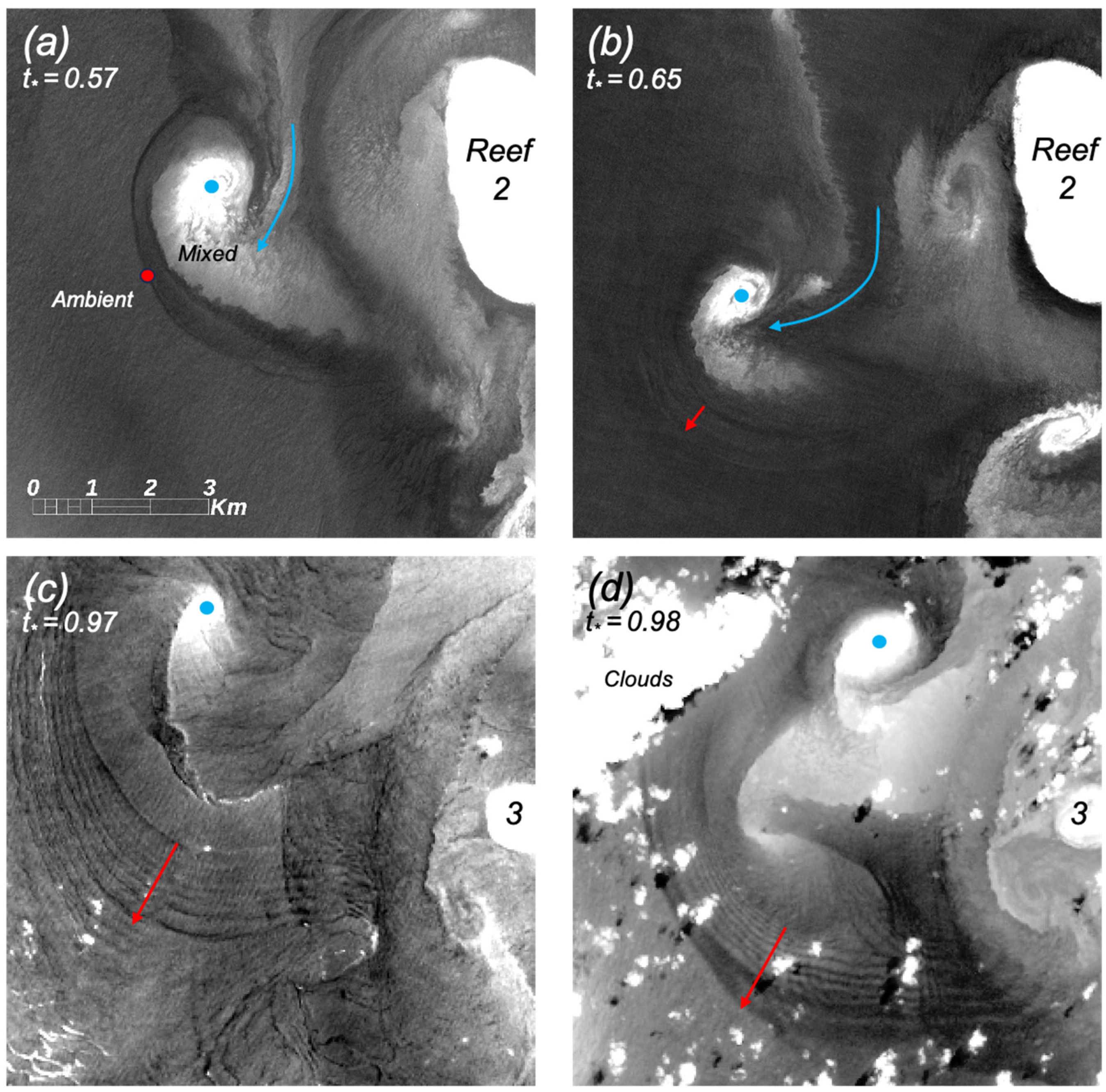
We further explore the above conjecture through a comparison of two mid-flood cases and two high-tide cases (Figure 9). The mid-flood cases (upper row) have comparable flood-tide height ranges (4.19 m and 4.37 m), but the second case occurs 0.53 h later in the flood cycle. Both cases reveal a similar localized flow between reefs 1 and 2, feeding into a vortex-frontal feature. A difference between the two cases is that in place of the earlier solitary, curved dark band in Figure 9a, Figure 9b shows (albeit faintly) evidence of several curved dark bands. Under the assumption these bands are internal waves or the beginnings of internal waves, they are marked with a short red arrow to indicate propagation direction. Note these bands extend farther from the vortex-frontal feature than the earlier solitary band, which would be consistent with wave propagation. As for the two high-tide cases (lower row), each shows a nearly semi-circular packet containing 8 to 10 waves and propagating toward the southwest. Features lie slightly farther south in Figure 9d, likely because that case had the stronger tidal forcing—a range of 4.42 m vs. 3.5 m for Figure 9c.
A hypothesis, then, is that the wave packets in Figure 9c,d are generated locally from the vortex-frontal feature and that they grow over the three hours between mid-flood and high tide. The occurrence of multiple wave packets in a single image (e.g., Figure 4 and Figure 7) with a spacing of about 7 km would be consistent with tidal generation from this single source acting in successive flood tidal cycles, though it is also possible there are multiple source locations. Just how the waves might be generated is discussed next.
4.1.2. Frontal Intrusion as a Generating Mechanism
A train of solitary internal waves can be created by the gravitational collapse of a mixed region in a stratified fluid [8]. This is a “dam break” problem, in which a volume of mixed fluid of density ρ2 is released into a two-layer system having vertical density difference Δρ = ρ3 − ρ1. Maxworthy [8] found that as long as the ambient fluid is capable of supporting internal wave motions, such motions will invariably arise from almost any form of mixing process. In our case, the mixing process is the turbulent stirring of the water column by tidally driven flow past the reefs, and this creates a water mass denser than the ambient near-surface layer (ρ1) but less dense than the ambient lower layer (ρ3). This mixed fluid intrudes into the ambient thermocline beneath the surface front separating the mixed and ambient water masses; a first wave will then form near the forward-most part, or head, of the intrusion. Possibly, the solitary dark bands in the mid-flood imagery (e.g., Figure 9a) are evidence of this initial wave, with additional waves forming subsequently (Figure 9b).
The gravitational collapse of mixed fluids forced by across-front velocity has been investigated by Bourgault et al. [9]. For the two-dimensional case, several different initial conditions for velocity and water density were examined, including ones having no across-front velocity. While the amplitude of the solitary waves formed varied considerably, all cases showed that the head of the intrusion continuously emits waves, one wave being emitted roughly every six buoyancy periods. The buoyancy period is given by τ = 2π/N, where N = [g (Δρ/ρ0)/h]1/2 is the buoyancy frequency in the ambient water, g being the gravitational acceleration. While the dynamical settings are not identical, we can try applying their result to our situation. Using Δρ/ρ0 ~ 4.5 × 10⁻⁴ (Section 3.1) and a thermocline thickness h~10 m (Section 3.2) yields a value for τ of about 5 min; so, one internal wave would be emitted every 30 min. In the interval between mid-flood and high tide, one might thus expect six waves to have formed. While Figure 9 shows more waves than this (about ten), the mechanism of gravitational collapse seems a plausible candidate for generating the internal waves we see, though obviously, further investigation is needed.
4.2. Possible Ecological Significance
Given the relative rarity of imagery of internal waves in the study area, one may wonder just how often internal waves do occur and whether that is often enough for them to play any significant role. The likelihood of occurrence of internal waves can be addressed by estimating how many internal wave-favorable days are likely in a given year. Using a conservative criterion ΔT > 1 °C as a proxy for favorable conditions, it is found that over the period of 2015 through 2023, the number of favorable days ranged from a low of 11 to a high of 75 per year, with a mean value of 40.6 (s.d. = 18.1). Also, favorable days usually occur as runs of consecutive days; these range in length from 5 to 43 days, with a mean of 19 days (s.d. = 12 days). Runs increase the chances of detecting internal waves, as more waves are likely to be generated and accumulate over time. As indicated in Section 3.1, favorable days occur predominantly in austral spring and summer seasons, i.e., the months of September to November and December to February. During that half-year period, the probability of a favorable day occurring is about 22%, though not every favorable day may exhibit internal waves (Section 3.1). Still, the conditions under which internal waves might be found are not as infrequent as the imagery search suggests. Also, while no systematic examination was made of other parts of the lagoon, it was clear while examining the cases in Table 1 that internal waves also occurred well outside the study area (an example is shown in the Graphical Abstract for Calder Island, about 45 km west-northwest of reef 1). This suggests that when conditions are favorable, internal waves can occur broadly.
Can the internal waves be of any ecological significance? The bloom-forming cyanobacterium Trichodesmium plays a key role in the biogeochemistry of the GBR lagoon because of its ability to fix nitrogen. In the south GBR lagoon, blooms of Trichodesmium occur in October and November, with the largest surface aggregations associated with low wind speed (<6 m/s) and surface water warmer than 24 °C [10]. These conditions are favorable for the occurrence of internal waves in the lagoon. Indeed, the area of high chlorophyll-a in Figure 8 is likely cyanobacteria, as are the prominent surface aggregations in Figure 4. Also, it is in October and November when corals inject large amounts of larvae into the water. The larvae are buoyant and, in winds under 5 m/s, aggregate into long surface slicks that are closely associated with tidally generated vortices, jets, and fronts [11,12]. While not previously considered, internal waves occurring during such spawning periods may be of some significance as an agent for the dispersal and transport of the larvae. Finally, there is the potential role of internal waves in cooling reef habitats that lie near the thermocline depth [13], but as most reefs lie seaward of the lagoon, any effect would likely be quite limited.
5. Conclusions
In summary, we have presented evidence that internal waves do indeed occur in the lagoon. The following conclusions can be drawn:
- Favorable conditions for the occurrence of internal waves are a shallow stratification (thermocline centered at about 8 m depth) and low wind (usually 4 m/s or less).
- Those conditions may not be sufficient, however, as some favorable days do not have visible internal wave signatures.
- At least some internal wave packets appear to be generated locally through a link with tidally forced submesoscale jets and vortices, but the actual mechanism generating the waves is unclear.
- As the internal waves occur during austral spring and summer, they may play some role in the dispersion and transport of cyanobacteria and planktonic larvae.
This study has been an exploratory first step, and further investigation is needed. This could be a broadening of scope to other parts of the lagoon; conducting in situ experiments to examine additional aspects of the waves, such as their amplitude, propagation speed, and longevity; and testing ideas about how the waves are generated.
Supplementary Materials
The following supporting information can be downloaded at: https://www.mdpi.com/article/10.3390/rs16122180/s1, Figure S1: Sentinel-1 synthetic aperture radar image of the study area; Figure S2: Representative temperature profile at the time of the SAR image.
Funding
This research was funded by the Office of Naval Research.
Data Availability Statement
Data are publicly available as described in the text.
Acknowledgments
This is contribution NRL/JA/7233--0079-24.
Conflicts of Interest
The author declares no conflicts of interest.
References
- Wolanski, E.; Kingsford, M.; Lambrechts, J.; Marmorino, G. The Physical Oceanography of the Great Barrier Reef: A Review. In Oceanographic Processes of Coral Reefs Physical and Biological Links in the Great Barrier Reef, 2nd ed.; Wolanski, E., Kingsford, M.J., Eds.; CRC Press: Boca Raton, FL, USA, 2023; Chapter 2; 26p. [Google Scholar] [CrossRef]
- Luick, J.L.; Mason, L.; Hardy, T.; Furnas, M.J. Circulation in the Great Barrier Reef Lagoon using numerical tracers and in situ data. Cont. Shelf Res. 2007, 27, 757–778. [Google Scholar] [CrossRef]
- Mao, Y.; Ridd, P.V. Sea surface temperature as a tracer to estimate cross-shelf turbulent diffusivity and flushing time in the Great Barrier Reef lagoon. J. Geophys. Res. Ocean. 2015, 120, 4487–4502. [Google Scholar] [CrossRef]
- Delandmeter, P.; Lambrechts, J.; Marmorino, G.O.; Legat, V.; Wolanski, E.; Remacle, J.F.; Chen, W.; Deleersnijder, E. Submesoscale tidal eddies in the wake of coral islands and reefs: Satellite data and numerical modelling. Ocean Dyn. 2017, 67, 897–913. [Google Scholar] [CrossRef]
- Jackson, C.R.; da Silva, J.C.B.; Jeans, G. The generation of nonlinear internal waves. Oceanography 2012, 25, 108–123. [Google Scholar] [CrossRef]
- Marmorino, G. Investigation of Turbulent Tidal Flow in a Coral Reef Channel Using Multi-Look WorldView-2 Satellite Imagery. Remote Sens. 2022, 14, 783. [Google Scholar] [CrossRef]
- Jackson, C.R.; da Silva, J.C.B.; Jeans, G.; Alpers, W.; Caruso, M.J. Nonlinear internal waves in synthetic aperture radar imagery. Oceanography 2013, 26, 68–79. [Google Scholar] [CrossRef]
- Maxworthy, T. On the formation of nonlinear internal waves from the gravitational collapse of mixed regions in two and three dimensions. J. Fluid Mech. 1980, 96, 47–64. [Google Scholar] [CrossRef]
- Bourgault, D.; Galbraith, P.S.; Chavanne, C. Generation of internal solitary waves by frontally forced intrusions in geophysical flows. Nat. Commun. 2016, 7, 13606. [Google Scholar] [CrossRef] [PubMed]
- Blondeau-Patissier, D.; Brando, V.; Lønborg, C.; Leahy, S.; Dekker, A. Phenology of Trichodesmium spp. blooms in the Great Barrier Reef lagoon, Australia, from the ESAMERIS 10-year mission. PLoS ONE 2018, 13, e0208010. [Google Scholar] [CrossRef] [PubMed]
- Oliver, J.K.; Willis, B.L. Coral-spawn slicks in the Great Barrier Reef: Preliminary observations. Mar. Biol. 1987, 94, 521–529. [Google Scholar] [CrossRef]
- Pattiaratchi, C. Physical oceanographic aspects of the dispersal of coral spawn slicks: A review. Bio-Phys. Mar. Larval Dispersal 1994, 45, 89–105. [Google Scholar]
- Wyatt, A.S.J.; Leichter, J.J.; Toth, L.T.; Miyajima, T.; Aronson, R.B.; Nagata, T. Heat accumulation on coral reefs mitigated by internal waves. Nat. Geosci. 2020, 13, 28–34. [Google Scholar] [CrossRef]
Figure 1.
(a) Bathymetry for the southern section of the GBR. Red rectangle shows study area. (b) Enlargement of study area. Numbers identify particular reefs: 1, Tern Reef; 2, Bushy-Redbill Reef; 3, Sandpiper Reef; 4, Prince Reef; and 5, Alarm Reef. (c) A Sentinel-2 satellite image of the study area, showing tidally generated vortices, as revealed by patterns of re-suspended sediment. Image data are from 28 March 2021, acquired at the end of a flood tide and under a north wind of about 8 m/s.
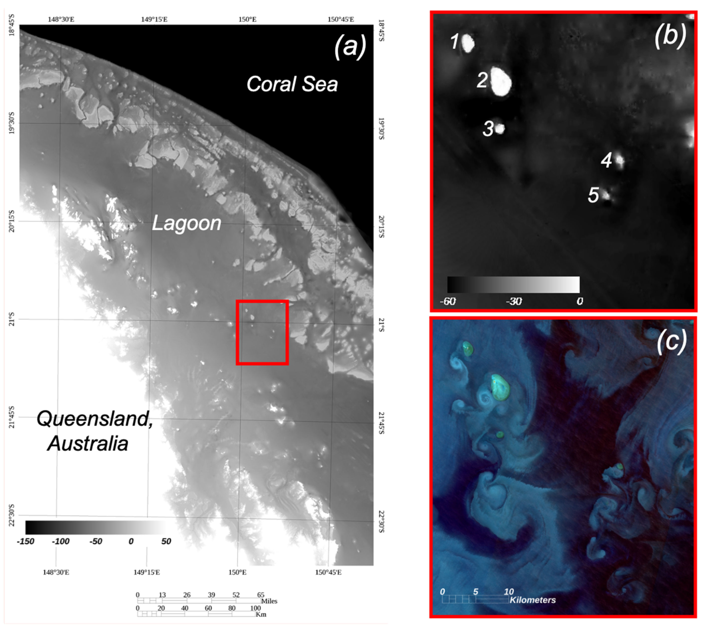
Figure 2.
Values of eReefs model wind speed and water stratification ΔT for year 2022. Daily mean values are shown; ΔT is the temperature at 2.4 m depth minus that at 49.0 m. Black vertical lines in the ΔT panel indicate occurrences of internal waves (cases 15 to 19, Table 1); horizontal black line indicates a threshold value of 0.75 °C.
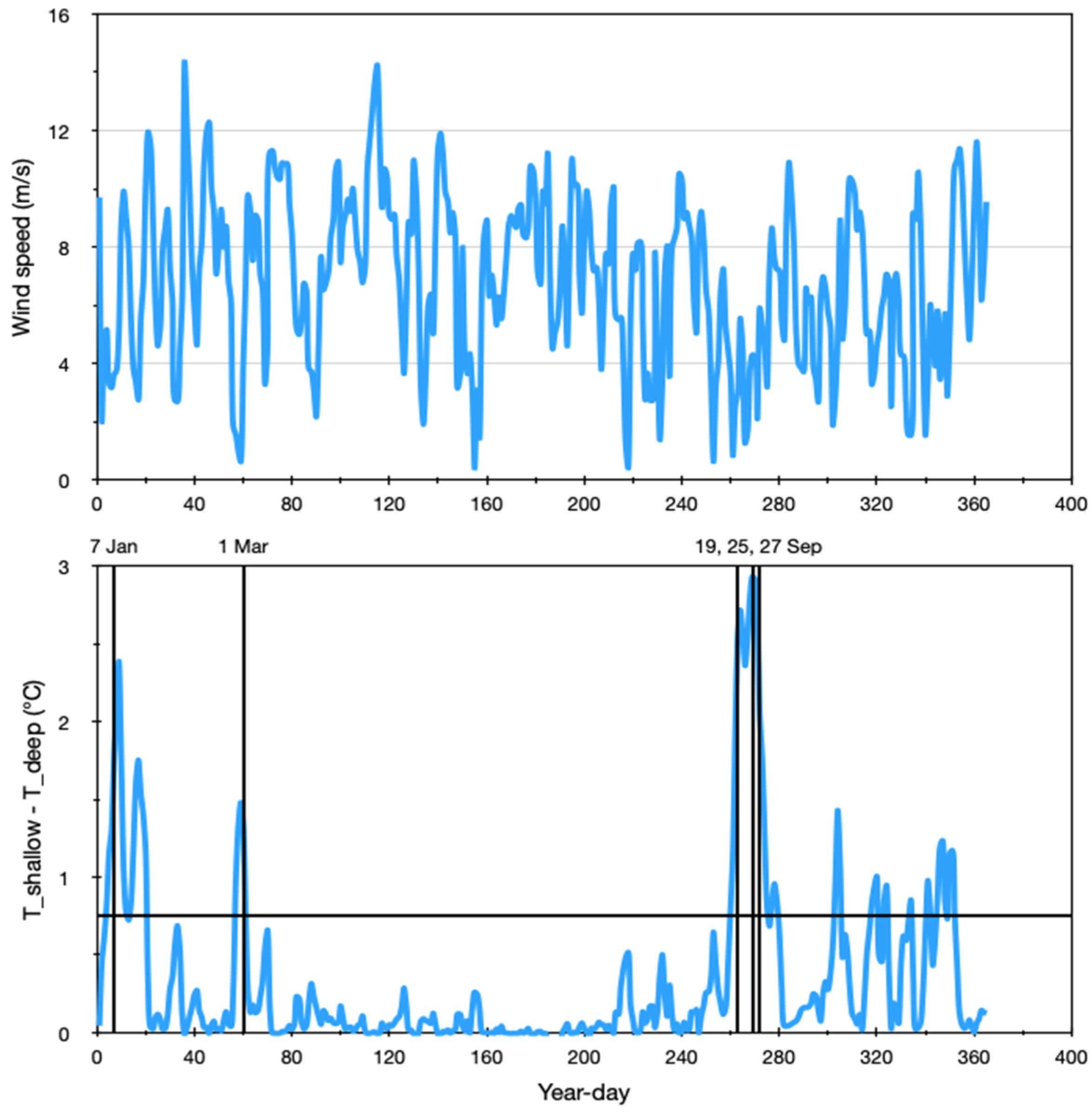
Figure 3.
(a) Temperature profiles corresponding to cases 2, 10, 17, and 18 (Table 1). Data are eReefs hourly mean values at 10:00 a.m. local time. As the lower layer is homogeneous, only the upper half of the water column is shown. (b) Evolution of the temperature profile for case 18 over 15 h, from 7:00 p.m. of the previous evening to 10:00 a.m.
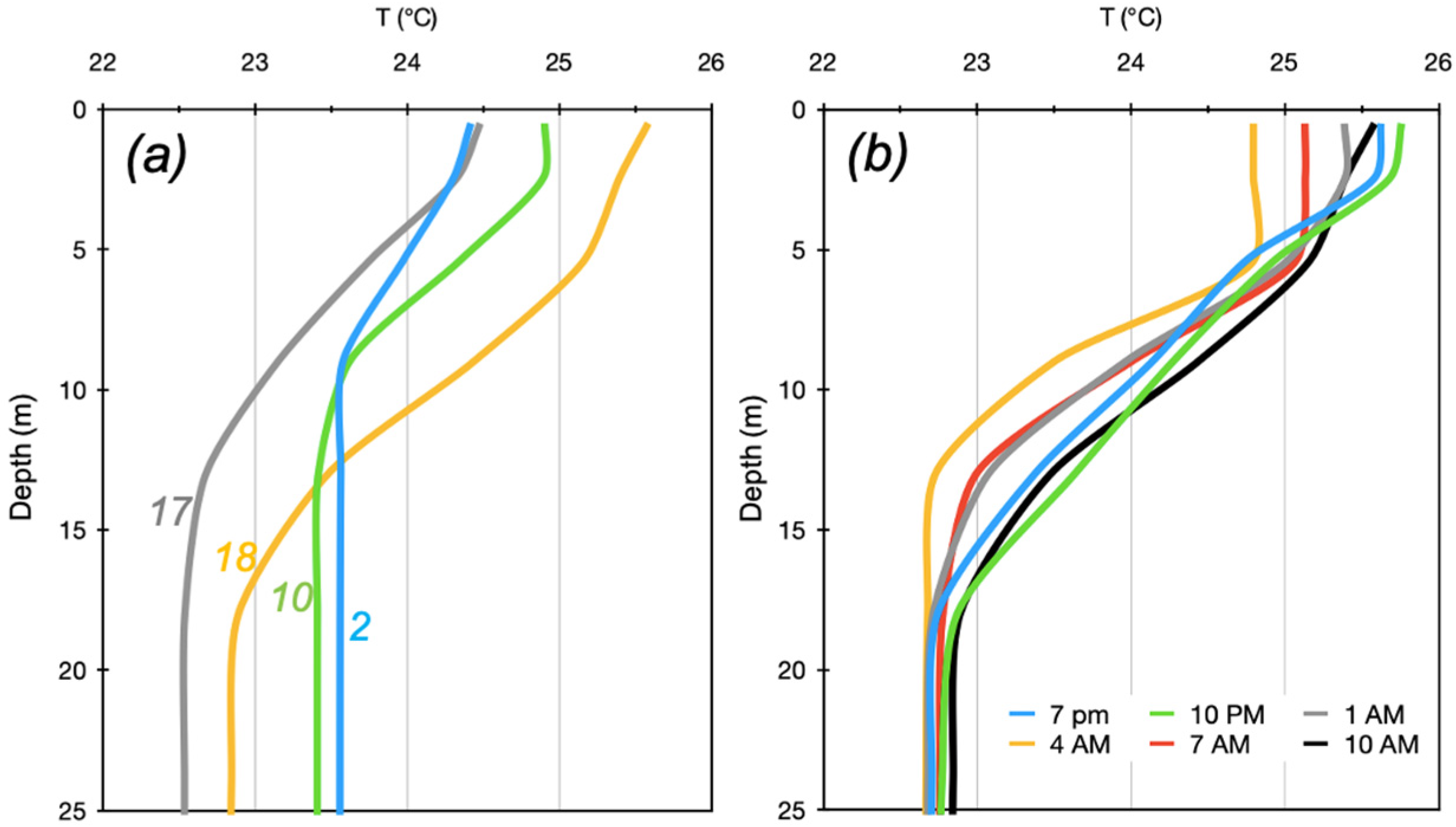
Figure 4.
Conditions around reefs 1–3 during low tide on 24 September 2020 (Case 10 of Table 1). The image has been contrast-stretched to emphasize the internal waves. Vector (upper right) shows eReefs hourly current at 0.5 m depth. Clouds predominate in the upper-right part of the image. Red arrows indicate local internal wave propagation direction.
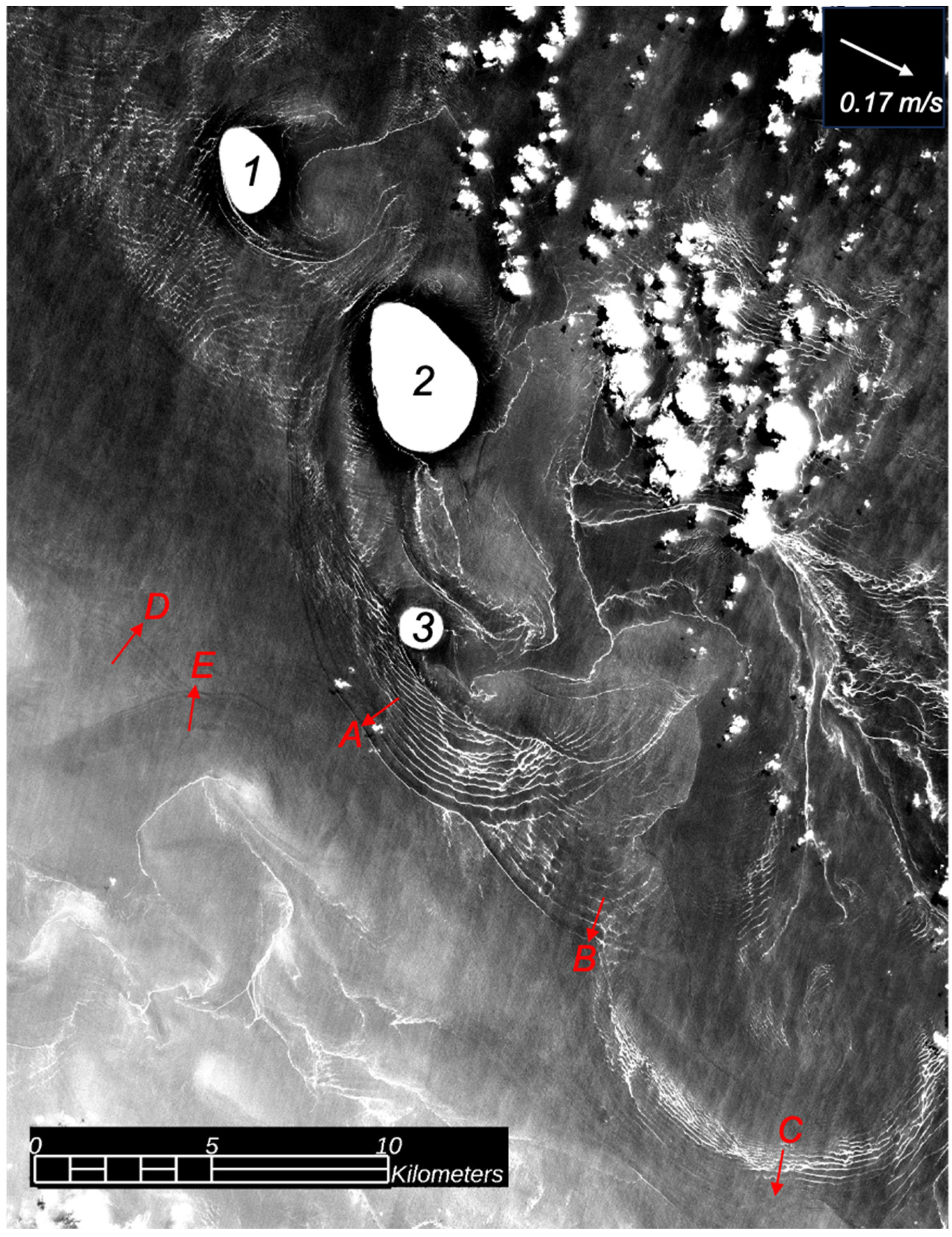
Figure 5.
Internal wave packet south of reef 3, enlarged from previous figure. A transect made along the red line (inset) shows a general trend of decreasing wavelength behind the leading wave. To reduce noise, the data have been averaged over 25 pixels (250 m) in the across-transect direction; varying peak heights are of no significance. Three thick line segments in the plot correspond to trailing-edge dark bands (see text).
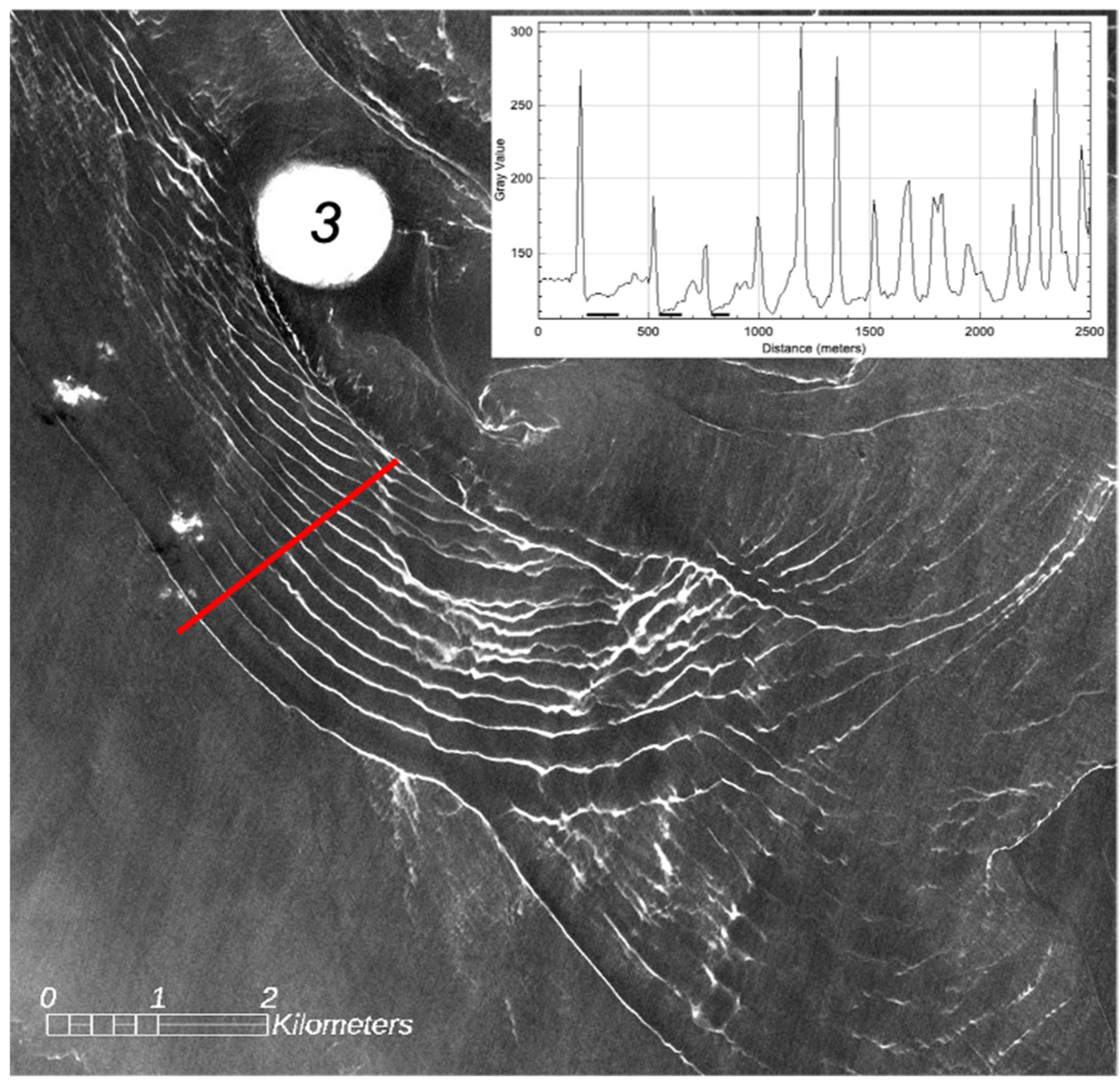
Figure 6.
As in Figure 4, but during the middle of a flood tide on 20 September 2016 (Case 2 of Table 1). Clouds appear across the lower part of the image. Hypothetical flow patterns are indicated by cyan-colored arrows. Features 1–4 are narrow dark bands.
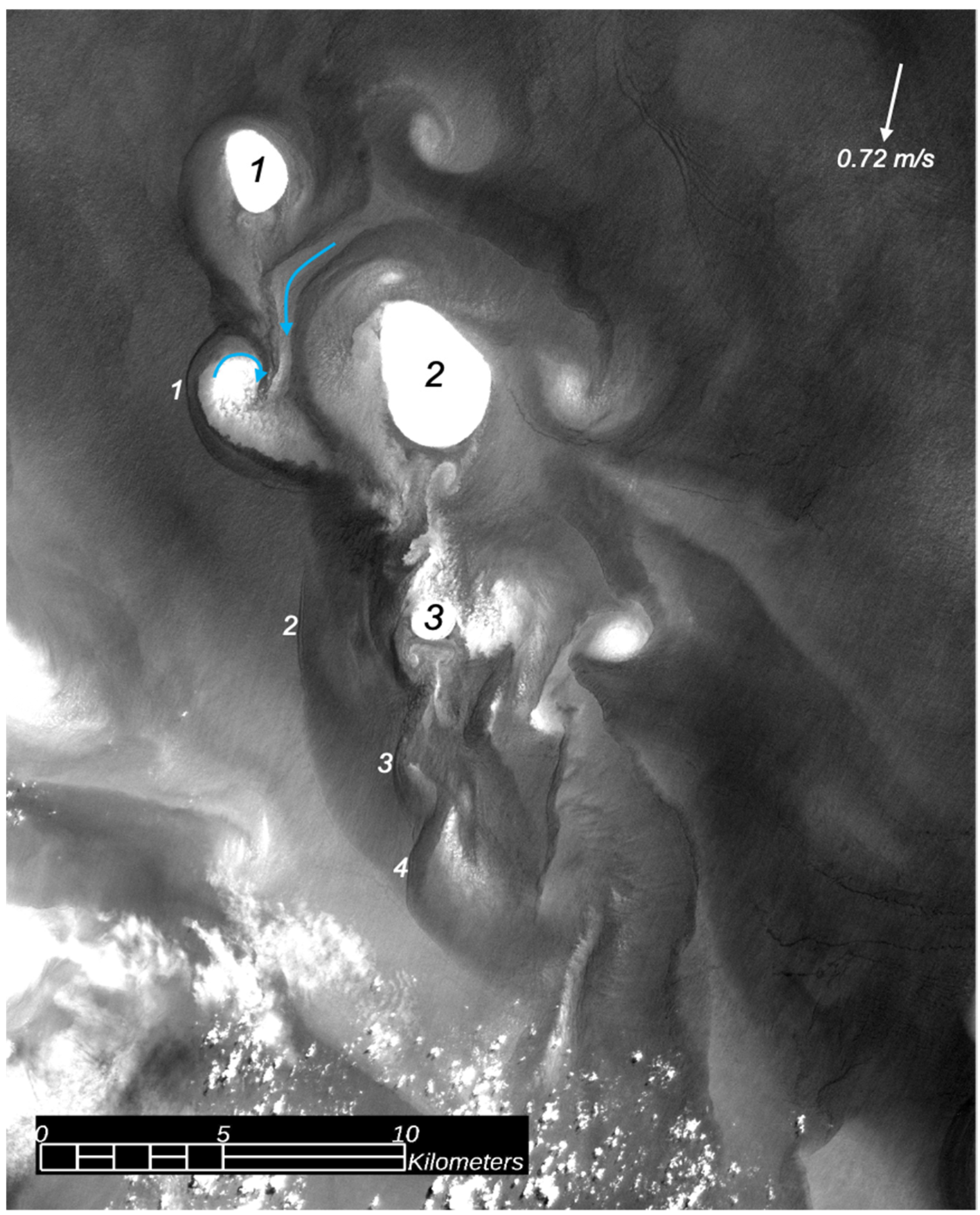
Figure 7.
As in Figure 4, but during high tide on 25 September 2022 (Case 18 of Table 1). Small clouds are scattered across the lower-left part of the image.
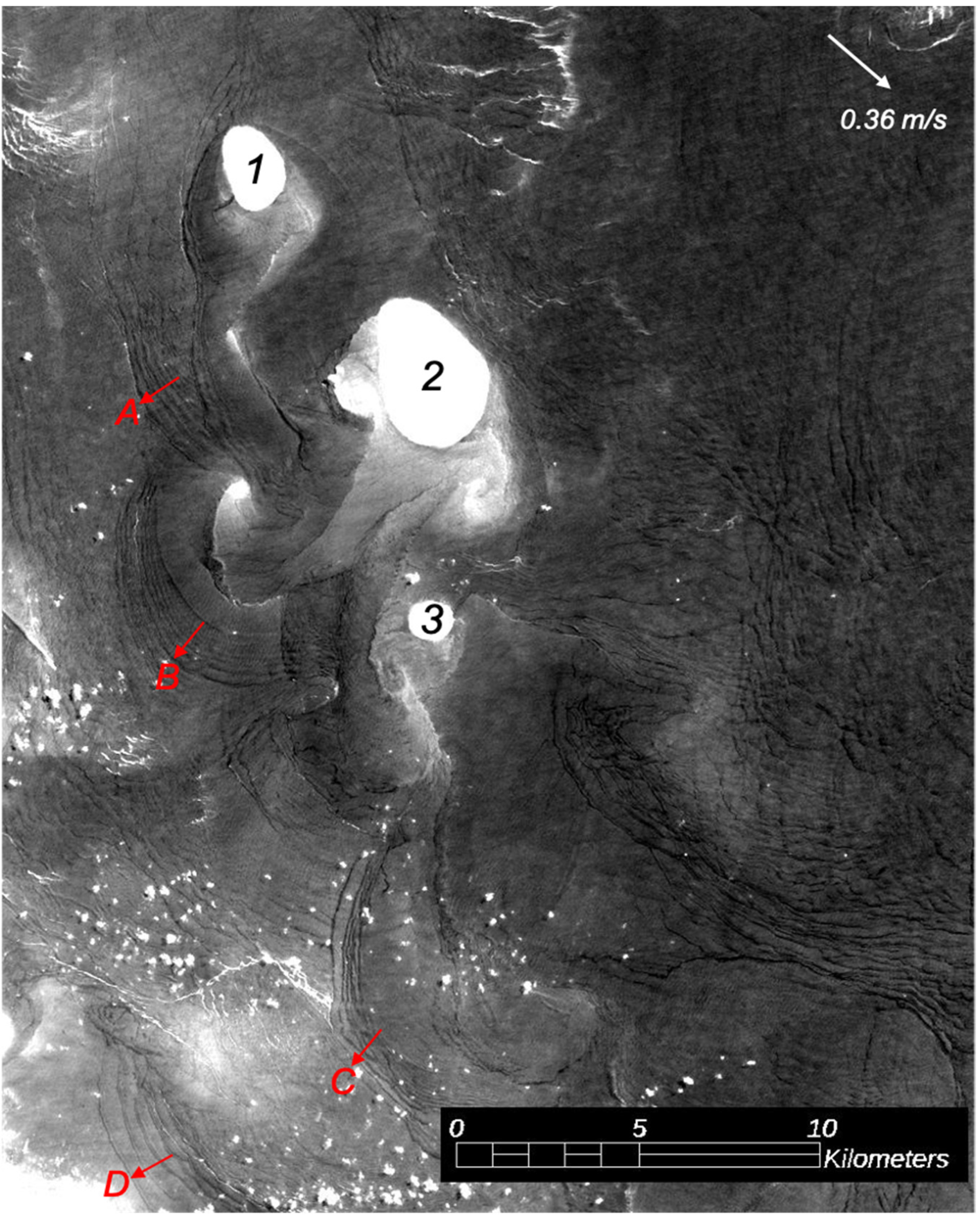
Figure 8.
(a) Sentinel-2 image of the entire study area at 10:13 AEST on 19 September 2022, about one hour before low tide (Case 17 of Table 1). Vector shows eReefs hourly current at 0.5 m depth. (b) Nearly coincident chlorophyll-a concentration, as measured by the Ocean and Land Color Instrument aboard the Sentinel-3 satellite. Data were acquired at 09:26 AEST on 19 September 2022 and have a spatial resolution of 300 m. Brightest water areas in the Sentinel-2 image correspond to areas of highest chlorophyll-a concentration of about 1 mg/m3 (areas in yellow); red areas result from shallow-water algorithm errors. (c) Enlargement of area highlighted in panel (a), showing conditions around reefs 4 and 5. Red arrows indicate the propagation direction of several internal wave packets.
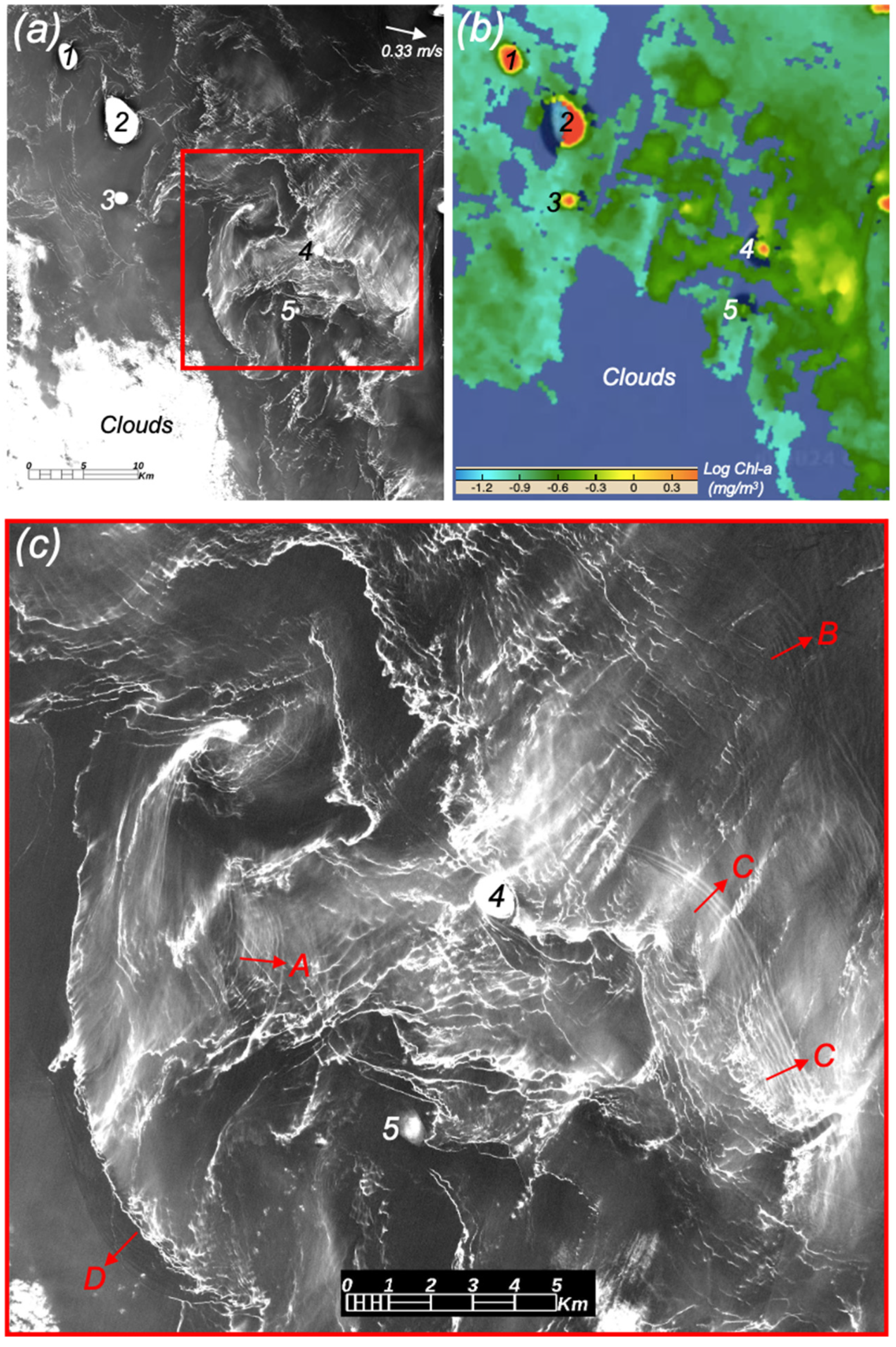
Figure 9.
Imagery near reefs 2 and 3 during flood (upper row) and at high tide (lower row). (a) Sub-area from Figure 6 (Case 2). (b) Same area but for case 12. (c) Sub-area from Figure 7 (Case 18). (d) Same area but for Case 1. As the duration of flood tide is variable, a non-dimensional time t* is used to indicate the progression from low (t* = 0) to high water (t* = 1). Each panel is 9 km by 9 km in extent; length-scale bar given in panel (a). Hypothetical flow patterns and vortex indicated by cyan color; internal waves, by red arrows; possible incipient internal wave, by red dot.

Table 1.
Satellite overpasses that show internal waves in the study area, along with environmental parameters at the approximate time of each overpass. AEST is Australian Eastern Standard Time, which is ten hours ahead of UTC. Current speed is at 0.5 m depth; ΔT is the temperature at 2.4 m depth minus that at 49.0 m. Values are eReefs model-derived hourly averages. Cases for which imagery is presented are indicated in the final column; case 14 is shown in the Supplementary Material.
| Case | Satellite | Overpass Time [AEST] | Tidal Phase | Current [m/s] | Wind [m/s] | ΔT [°C] | Figure |
|---|---|---|---|---|---|---|---|
| 1 | Landsat-8 | 2015 Aug 29 09:58 | High water | 0.40 | 4.1 | 0.43 | 9 |
| 2 | Sentinel-2 | 20 September 2016 10:12 | Flood | 0.72 | 3.2 | 0.85 | 6,9 |
| 3 | Landsat-8 | 8 December 2017 09:59 | Flood | 0.64 | 3.5 | 1.45 | |
| 4 | Sentinel-2 | 20 October 2018 10:11 | Ebb | 0.29 | 3.4 | 1.01 | |
| 5 | Sentinel-2 | 12 February 2019 10:13 | Low water | 0.42 | 4.8 | 1.07 | |
| 6 | Landsat-8 | 13 February 2019 09:59 | Ebb | 0.34 | 3.0 | 1.34 | |
| 7 | Sentinel-2 | 14 March 2019 10:22 | Low water | 0.33 | 2.7 | 0.75 | |
| 8 | Sentinel-2 | 23 January 2020 10:13 | High water | 0.36 | 3.8 | 2.46 | |
| 9 | Sentinel-2 | 15 August 2020 10:13 | Ebb | 0.55 | 2.6 | 0.54 | |
| 10 | Sentinel-2 | 24 September 2020 10:13 | Low water | 0.17 | 1.0 | 1.49 | 4,5 |
| 11 | Sentinel-2 | 23 December 2020 10:13 | Ebb | 0.35 | 2.8 | 1.38 | |
| 12 | Sentinel-2 | 9 October 2021 10:13 | Flood | 0.70 | 5.4 | 0.77 | 9 |
| 13 | Landsat-9 | 11 December 2021 09:59 | Low water | 0.28 | 2.5 | 3.53 | |
| 14 | Sentinel-1 | 24 December 2021 05:28 | Low water | 0.16 | 2.3 | 1.25 | S1 |
| 15 | Sentinel-2 | 7 January 2022 10:13 | Flood | 0.67 | 2.3 | 1.58 | |
| 16 | Landsat-9 | 1 March 2022 09:59 | High water | 0.26 | 2.8 | 1.20 | |
| 17 | Sentinel-2 | 19 September 2022 10:13 | Ebb | 0.33 | 1.8 | 1.80 | 8 |
| 18 | Landsat-9 | 25 September 2022 09:59 | High water | 0.36 | 4.0 | 2.57 | 7,9 |
| 19 | Sentinel-2 | 27 September 2022 10:23 | Flood | 0.63 | 3.6 | 2.54 |
Disclaimer/Publisher’s Note: The statements, opinions and data contained in all publications are solely those of the individual author(s) and contributor(s) and not of MDPI and/or the editor(s). MDPI and/or the editor(s) disclaim responsibility for any injury to people or property resulting from any ideas, methods, instructions or products referred to in the content. |
© 2024 by the author. Licensee MDPI, Basel, Switzerland. This article is an open access article distributed under the terms and conditions of the Creative Commons Attribution (CC BY) license (https://creativecommons.org/licenses/by/4.0/).
Share and Cite
MDPI and ACS Style
Marmorino, G. A First Look at Internal Waves in the Great Barrier Reef Lagoon. Remote Sens. 2024, 16, 2180. https://doi.org/10.3390/rs16122180
AMA Style
Marmorino G. A First Look at Internal Waves in the Great Barrier Reef Lagoon. Remote Sensing. 2024; 16(12):2180. https://doi.org/10.3390/rs16122180
Chicago/Turabian StyleMarmorino, George. 2024. "A First Look at Internal Waves in the Great Barrier Reef Lagoon" Remote Sensing 16, no. 12: 2180. https://doi.org/10.3390/rs16122180
Note that from the first issue of 2016, this journal uses article numbers instead of page numbers. See further details here.