From Dawn to Dusk: High-Resolution Tree Shading Model Based on Terrestrial LiDAR Data

Abstract

Light availability and distribution play an important role in every ecosystem as these affect a variety of ecosystem processes and functions. To estimate light availability and distribution, light simulations can be used. Many previous models were based on highly simplified tree models and geometrical assumptions about tree form, or were sophisticated and computationally demanding models based on 3D data which had to be acquired in every season to be simulated. The aim of this study was to model the shadow cast by individual trees at high spatial and temporal resolution without the need for repeated data collection during multiple seasons. For our approach, we captured trees under leaf-off conditions using terrestrial laser scanning and simulated leaf-on conditions for individual trees over the remainder of the year. The model was validated against light measurements ($n=\mathrm{20,436}$) collected using 60 quantum sensors underneath an apple tree (Malus domestica Borkh.) on a sunny and cloudless summer day. On this day, the leaves and the shadow were simulated with a high spatial (1 cm) and temporal resolution (1 min). The simulated values were highly correlated with the measured radiation at $r=0.84$. Additionally, we simulated the radiation for a whole year for the sample apple tree (tree height: 6.6 m, crown width: 7.6 m) with a resolution of 10 cm and a temporal resolution of 10 min. Below the tree, an area of 49.55 m² is exposed to a radiation reduction of at least 10%, 17.74 m² to at least 20% and only 0.12 m² to at least 30%. The model could be further improved by incorporating branch growth, curved leaf surfaces, and gravity to take the weight of the foliage into account. The presented approach offers a high potential for modelling the light availability in the surroundings of trees with an unprecedented spatial and temporal resolution.

1. Introduction

Light availability, distribution, and spectral composition are environmental factors that play a critical role in ecosystems. For plants, light availability is the main driver of photosynthesis and it controls the net assimilation rate, which in turn drives biomass production. The available solar radiation, the length of the growing season and the available leaf area are limiting plant growth, when plants are not limited in their growth by nutrients or water [1,2]. Conversely, excessive light can also cause light stress in some species, depending on their shade tolerance [3]. The spectral composition of light, sometimes referred to as light quality, also influences plant growth and development [4,5]. On the ecosystem level, light availability influences species composition and diversity [6,7]. On the microclimatic level, a number of environmental parameters and processes, including soil temperature and moisture, air humidity, and evapotranspiration are sensitive to light availability [8]. These microclimatic conditions can in turn significantly impact ecosystem processes and biodiversity [9]. Besides light availability, spatial light heterogeneity also evidently plays a role in species diversity [10]. However, not only the spatial but also the temporal variation of radiation is crucial to ecosystems. Sun flecks, i.e., the short and small-scale occurrence of high radiation intensity, are crucial for the carbon fixation of shaded leaves and understory vegetation on both the daily and annual scales [11]. Measuring light at high spatial and temporal scales could thus improve our understanding of ecosystem dynamics and processes in various ecosystems [9].

Agroforestry systems (AFS) are one type of agricultural management system where light availability is of particular importance. AFS can be defined as a combination of perennial woody plants such as trees and shrubs interacting with crop and/or livestock within the same management unit [12]. The interactive influence of the trees on the crop or livestock is highly relevant. The effects of tree shade on crop yields have been studied for a broad variety of silvoarable systems, i.e., AFS with crop production. While some studies found yields to decrease, especially with increasing shading intensity [13,14], other studies found no differences between shaded and non-shaded sites or even found yield increases [15,16]. Presumably, the extent of the shading effect depends on various factors, such as the type of crop and tree species, tree spacing and crown expansion, management, climate and soil type [17]. For silvopastoral systems, the positive impact of tree shade on livestock is well documented [18,19]. The reduction in livestock heat stress by the inclusion of trees on ranch land can serve as an adaptation strategy to climate change [20]. However, many farmers currently perceive shading by trees generally as a disadvantage due to crop yield reduction concerns [21]. This perception could change for the better in the context of climate change, rising temperatures, and resulting challenges in crop yield maintenance.

Light availability in ecosystems is typically measured directly or indirectly at specific points in time or space. For example, hemispherical photos can be used to assess the availability of light in forests indirectly via photographing the sky from the ground using an ultra-wide angle or fish-eye lens. The images are then analysed to assess canopy characteristics that allow conclusions to be drawn about light availability [22,23]. The leaf area index (LAI), a ratio between the leaf and the ground area, is another indirect approach to estimate light availability [4,24]. LAI sensors measure the light transmission through a canopy at defined points or along transects [25]. Engelbrecht and Herz [26] compared direct and indirect light measurements. They concluded that indirect light measurements are not sufficient to measure light accurately. Quantum sensors can be used to measure light directly and with high accuracy. However, direct measurements with quantum sensors are expensive and time-consuming, especially when covering large areas [26]. All of these methods for estimating or measuring light may vary in their accuracy, but all demonstrate spatial and/or temporal limitations in their application.

An alternative to in-situ light measurements are light simulation approaches. Light simulations neither require the maintenance of a sensor network over long time periods nor replicated measurement campaigns over the season. When the shape and location of any object are known, its shadow can be calculated. However, for objects with complex structures such as trees, the simulation of shade is less straightforward. Especially for large trees which comprise thousands of leaves and branches, shade mapping is challenging. Nevertheless, simulations have the big advantage of the fact that shadow can be mapped at any desired point in time and space. However, many light simulations involving trees that are either kept simple and are based on simple geometric assumptions or are very complex and aim to model shading as realistically as possible. The complexity of the light models varies both in terms of the geometric representation of the trees and the underlying light simulation algorithms. The simpler models rely on a small number of geometric primitives such as cylinders, cones, and ellipsoids to represent tree trunks and crowns and use simple algorithms to calculate shadows [27,28,29,30]. At the other end of the spectrum are sophisticated models that require high-resolution 3D data from trees and use complex algorithms such as ray tracing or radiative transfer models [31,32]. While simple models are limited in their accuracy, complex models are computationally demanding and require 3D data from all seasons to simulate light availability over the course of a year. Depending on the objective of the model application, either a simple or a complex model may be advantageous. To estimate the approximate size of tree shading and if 3D data are unavailable, simple models may be preferable. If the aim is to model microclimate, for example, and high-resolution 3D data are available, complex models are required. When modelling light availability in AFS, neither of these extremes of model complexity are desirable. Very simple models are likely to overestimate shading [27] or fail to map shading heterogeneity [29] due to the lacking inclusion of crown structure and architecture. Very complex models, on the other hand, are likely to be too costly due to the high computational and data requirements [30,33].

For the light simulation in AFS, it may better to use models that fall between these extremes in terms of complexity, e.g., approaches that use complex tree models but simple shading algorithms. To represent the complex structures of the trees, terrestrial laser scanning (TLS) can be used. TLS produces dense, high quality point clouds and is frequently used in forestry sciences to capture and analyse the various aspects of individual trees or forest stands [34,35,36,37]. A typical application of TLS in forestry is the derivation of forest inventory attributes such as tree position, stem diameter and height [38]. TLS can also be used to estimate parameters that are difficult or impossible to obtain from traditional field measurements, such as intricate branching structures [34,39]. More advanced tree-related TLS applications include species identification, stem quality assessment, and micro-habitat mapping [34]. In the field of agricultural sciences, TLS is currently considered impractical for surveying crops [40]. However, there have been horticultural studies using TLS to analyse fruit trees in orchards [41,42].

For many applications, it is necessary to simplify the complex 3D point clouds using parametric structural models. This simplification can be achieved, for example, through the use of quantitative structure models (QSMs). QSMs are simplified 3D models that represent the stem and branches of trees as a collection of geometric primitives, classically cylinders [43]. QSMs quantitatively describe the geometric, volumetric, and topological characteristics of individual trees [44]. A wide range of parameters can be derived from them, some of which are difficult or impossible to determine through fieldwork, such as whole tree volume and fine branching structures. As QSMs only represent the woody structures of trees, foliage would have to be simulated if light was to be simulated over the course of a whole year. This approach has been previously used by Rosskopf et al. [45], Bohn Reckziegel et al. [46] and Calders et al. [47]. They created leaf-off tree models using TLS and QSMs, simulated leaf-on conditions, and calculated the shade cast using geometric operations. The advantage of this approach is that data need to be collected only once under leaf-off conditions. However, Rosskopf et al. [45] represented the foliage as ellipsoids around the branches rather than simulating individual leaves. In the study by Bohn Reckziegel et al. [46], individual leaves were simulated, but the leaves were always oriented on a horizontal plane, which do not resemble realistic leaf angles. Calders et al. [47], on the other hand, used angled individual leaves but used a complex radiative transfer model that is computationally very demanding.

In this study, we present and validate an improved shading simulation based on TLS data and QSMs with simulated leaves. Our work represents an advance over previous approaches as we efficiently implemented realistically angled individual leaves and made our code available as an R package. Here, we validate our approach by scanning a deciduous tree in winter without leaves, measuring the radiation under the tree in summer with leaves, modelling the shade with simulated leaves, and comparing the measurements with the simulation. Furthermore, we simulate shade over a full year and combine it with radiation data to estimate the reduction in radiation under the sample tree over the course of a year.

2. Materials and Methods

In the following, the simulation process is explained, including the proposed data preparation. An overview of the entire workflow, from data acquisition to the final product of our leaf and shadow simulation, is shown in Figure 1. Next, the validation process is described. Finally, the simulation is applied to a single tree for a whole year as an example.

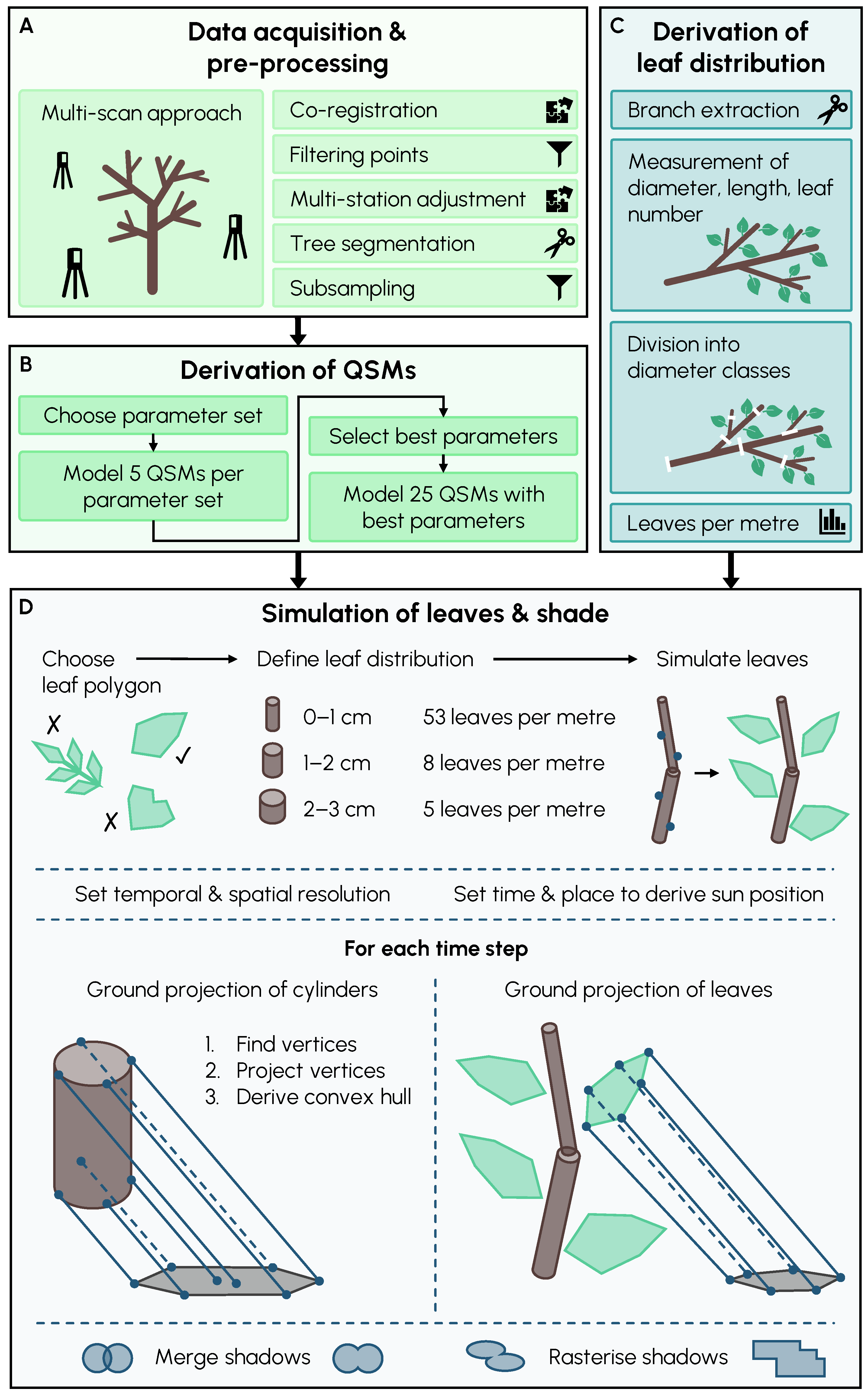
2.1. Simulation Workflow

2.1.1. Data Preparation

First, TLS data need to be acquired and pre-processed (Figure 1A). We recommend scanning trees from multiple directions to achieve the full coverage of all tree parts. The scans must then be co-registered with each other. It has been shown that multi-station adjustment can improve co-registration and the QSMs obtained in subsequent steps [48]. Furthermore, point clouds need to be filtered to remove noise. We also recommend filtering the points according to their range, as the quality of the point clouds decreases with increasing scanning distance [49]. The individual trees must be segmented from the point clouds and the ground must be removed. Depending on the resolution of the point cloud, it is recommended to subsample the point cloud to reduce the computational cost of the QSM derivation.

In order to reconstruct the QSMs (Figure 1B), we utilise TreeQSM v2.4.1 [44,50]. This is an established software that has already been validated several times [50,51,52]. TreeQSM is a library for Matlab (MathWorks, Natick, MA, USA) that is used to derive QSMs from single tree point clouds. The software uses an iterative and stochastic process to identify stem and branch segments and fit cylinders into them. TreeQSM requires the optimisation of several hyperparameters. The optimal hyperparameter values vary depending on various factors such as tree size and point cloud density [44]. To select the best hyperparameter values, an initial set of plausible values must be selected, then several models per hyperparameter combination must be calculated and compared. It is necessary to calculate multiple models because TreeQSM contains stochastic elements and produces different results at each model run. The developers suggest performing a simple grid search over the chosen hyperparameter space [44]. Typically, the best set of hyperparameters is determined by choosing the hyperparameter values that yield the smallest average distance between the 3D points and the fitted cylinders. Using the optimised hyperparameter values, a final set of QSMs must be calculated.

Next, the leaf distribution needs to be parameterised (Figure 1C). For this purpose, it is necessary to sample the branches of the studied tree species. The aim of the sampling is to determine the average number of leaves per metre of branch length in all relevant diameter classes. Typically, leaves are only attached to small diameter branches. Leaf density per diameter class can be determined in different ways. We suggest to perform a series of diameter and length measurements along with counting the leaves in order to categorise branches and corresponding leaves into branch diameter classes.

2.1.2. Simulating Leaves and Shade

The complete code for simulating the leaves and the shadow is written in R [53]. A package for reading QSMs from TreeQSM into R is available from https://github.com/zoeschindler/qsm2r (accessed on 23 May 2024) [54], while the leaf and shadow modelling is available at https://github.com/zoeschindler/qsm2shade (accessed on 23 May 2024) [55].

The leaf simulation process is shown in Figure 1D and explained in more detail in Appendix B. In the following, the algorithm is roughly outlined. The package uses the QSM of an individual tree as a starting point and models leaves onto the cylinders based on a specified leaf distribution. According to the leaf distribution, the number of leaves per cylinder is determined based on cylinder length and diameter. For the leaf shape, simple 2D polygons are used to maintain computational efficiency. The angle between the leaf surfaces and the ground can be set to any desired value.

For the shadow simulation, it is necessary to choose the desired temporal and spatial resolution. Theoretically, any spatial resolution and any temporal resolution down to seconds can be used. In practice, the resolution is limited by the length of the time series to be examined, the extent of the desired output raster and, above all, available computer memory. Next, the time frame and the location of the tree must be specified. This information is necessary to calculate the position of the Sun in relation to the tree for each time step. In the following steps, the program loops through the derived Sun positions and calculates shade cast of the woody tree parts and leaves for each time step.

The module for calculating the shadow is based on the tree’s woody biomass components, i.e., the stem and branches represented as leafless QSM. This follows the methodology introduced by Rosskopf et al. [45], adapted to increase computational efficiency. For a detailed description of the algorithm, see Rosskopf et al. [45]. In general, vertices on the top and bottom circles of the cylinders are obtained, the vertices are projected to the ground using parallel projection, and a convex hull is derived around the projected vertices of each cylinder. The main difficulty is to calculate the vertices that delimit the cylinder shadow on the ground. Projecting the leaves onto the ground is straightforward because the leaf polygons are 2D objects with a known order of vertices. Therefore, the vertices can be projected onto the ground and can simply be rearranged into polygons.

Finally, the shadows of all cylinders and leaves are merged and rasterised to the previously specified raster extent and resolution. For the rasterisation, the terra package [56] was used. The used function assigns polygon values to grid cells whose centres lie within the rasterised polygon. When additionally providing radiation data, shaded cells receive the diffuse radiation as a value, while non-shaded raster cells receive the global radiation sum as a value. If the aim is only to predict whether shading will occur, but not the light or shading intensity, it is sufficient to conduct the simulation without additional radiation data.

2.2. Model Validation

To validate our shadow simulation, we measured the radiation on the ground under an apple tree (Malus domestica Borkh.) on a cloudless summer day in August 2023 under leaf-on conditions using quantum sensors (hereafter referred to as “summer scan”). The setting was scanned with TLS to enable the accurate georeferencing of the quantum sensors. The same tree was scanned again in February 2024 to obtain data under leaf-off conditions (hereafter referred to as “winter scan”). The winter scan was spatially aligned with the summer scan and then used to create QSMs. The leaf simulation for apple trees was parameterized using additional leaf density data collected during a field work campaign in summer 2022. Using these data, the leaves and the shade were simulated with a spatial resolution of 1 cm and a temporal resolution of 1 min. Finally, the results of the simulation were compared with the sensor measurements.

2.2.1. Study Site

All parts of this study were conducted at sites close to Freiburg im Breisgau, in southwest Germany. Freiburg is located in the temperate oceanic climate zone (Köppen–Geiger: Cfb, [57]). The long-term average temperature between 1991 and 2020 was 11 °C, while the average annual rainfall sum was 896 mm [58]. The apple tree used for the validation of the shade and leaf model had no direct neighbouring trees and was managed in a similar way to an extensively managed orchard. At the time of the first data collection in August 2023, the tree had a diameter at breast height (DBH, measured at 1.3 m above the ground) of 19 cm, a height of 6.6 m, a crown base height of 2.1 m, an average crown width of 7.6 m and a crown projection area of 44.8 m². For the parameterisation of the simulated leaves, one to two branches each of 70 apple trees ($n=135$) located in five orchards near Freiburg were removed and examined. All these trees originated from systems similar to orchards. The trees had a DBH between 11 cm and 62 cm.

2.2.2. Terrestrial Laser Scanning

For both the summer and the winter scan, the apple tree was surveyed using TLS (Figure 1A). For both TLS campaigns, a RIEGL VZ-400i (RIEGL Laser Measurement Systems GmbH, Horn, Austria) terrestrial laser scanner was used. During both scanning operations, the tree was scanned from multiple positions around the tree to obtain a complete representation of the entire crown. After data acquisition, the scans were automatically registered and filtered in RiSCAN PRO v2.18.1 (RIEGL Laser Measurement Systems GmbH, Horn, Austria). As described below, the data were further processed in CloudCompare v2.12.4 (https://www.cloudcompare.org/ accessed on 23 May 2024). Figure 2 illustrates the processed single-tree point clouds from both scanning campaigns.

For the summer scan, we used a pulse repetition rate of 1200 kHz and an angular resolution of 0.04°. Since the quantum sensors were repositioned during the radiation data collection, the setup was scanned both before and after said sensor repositioning. The point clouds were filtered for isolated points (<5 neighbours in 10 cm radius), highly deviated points (deviation ≥ 15), dark points (reflectance ≤ −10 dB), and distant points (range > 15 m). The data of both setups were exported separately to CloudCompare, which was then utilised to manually georeference the quantum sensors.

For the winter scan, we employed a pulse repetition rate of 1200 kHz, but a higher angular resolution of 0.03°. We chose a higher resolution due to recent findings regarding the limitations of TLS and QSM for capturing fine branches [49]. Except for point brightness, the point clouds were filtered with the same settings. The point clouds were filtered less harshly for brightness (reflectance ≤ −15 dB) to ensure the high coverage of all woody structures. In addition, the registration of the scans was enhanced using the multi-station adjustment tool (MSA2), which has been shown to improve QSMs [48]. In CloudCompare, the ground and vegetation near the trunk were manually removed. To reduce noise, the statistical outlier removal tool was employed ($k=5$, $n=1$). This tool calculates the average distance of all points to their k nearest neighbours and removes points that are further away than the average distance plus n times the standard deviation. Finally, the point cloud was subsampled to a minimum point spacing of 5 mm and manually aligned to the summer point cloud.

2.2.3. Quantitative Structure Models

We employed TreeQSM v2.4.1 [44,50] to reconstruct QSMs from the filtered and subsampled winter scan (Figure 1B). We delineated a hyperparameter space based on previous experience. For each of the six resulting different hyperparameter sets, five QSMs were computed. The best hyperparameter set was selected based on the smallest average distance between the fitted cylinders and the point clouds. Using the optimised hyperparameter set, a final set of 25 QSMs was compiled. We derived multiple QSMs to later average the simulation results across all QSMs to account for the inherent uncertainties in the QSM reconstruction. To reduce the number of cylinders in the QSMs, these QSMs were simplified using a function contained in TreeQSM, which replaces two consecutive cylinders with a single cylinder. Figure 3 shows one of the final QSMs of the sampled apple tree.

2.2.4. Simulating Leaves and Shade

Data from 70 trees and 135 branches were used to parameterise the leaf distribution (Figure 1C). The branches were sourced from different crown sections and were randomly selected. For each branch, it was recorded whether it was from the lower, middle, or upper third of the crown and whether it was from the inner or outer crown layer. The outer crown layer was defined as the outer 2 m of the crown. The diameter of the branches’ cut faces ranged from 6 mm to 22 mm. Larger branches were not sampled because leaves were mainly attached to parts of branches with small diameters, and extracting larger branches could impact tree health and form. Each branch was divided into 1 cm diameter classes based on the length and diameter measurements using a caliper and tape measure. The number of leaves on the branches was counted and assigned to the different diameter classes. We compared leaf densities within the different crown sections, but found no large differences (see Figure A1). Therefore, the leaf density per branch length in the diameter classes was averaged over all measured branches, regardless of the crown sections from which the branches were sampled.

When simulating the leaves (Figure 1D) with the measured diameter distribution, the leaves were very sparsely distributed. This arises from the tendency of QSMs to overestimate the radii of the cylinders [48,49]. This effect is particularly strong for small branches because (1) they are typically further away from the TLS device during the scanning and the quality of the point cloud deteriorates with increasing scanning distance [49], and because (2) even small diameter overestimation on small branches leads to a large overestimation relative to their actual diameter [48]. To account for this cylinder inflation effect, we shifted the leaf density distribution by one class, i.e., the leaf density of class 0–1 cm was assigned to class 1–2 cm, and so on. After the diameter classes were shifted, the smallest diameter class that no longer had a leaf density was assigned its original value, so that this value was now assigned to the two smallest diameter classes. To derive the required leaf size, the length of several leaves in the summer scan was measured using CloudCompare. On average, the leaves had a length of 10 cm. Visual comparison between the summer point cloud and the winter QSM with simulated leaves showed good agreement. Figure 3 shows an example result of the leaf and shadow simulation for the sampled apple tree.

Table A1. Parameters used for the simulation. The tree location is described by “tree latitude” and “tree longitude”. The “spatial resolution” and “temporal resolution” give the respective simulation resolution. The “leaf width” and “leaf length” refer to the size of the leaf polygon. The “leaf stem length” refers to the length of the leaf petioles. The “leaf axis angle” refers to the angle of the leaf axis to the ground, with 0° being horizontal leaves and 90° being vertical leaves. The “leaf density” refers to the leaf density used for the cylinder diameter classes.

Simulation Parameter	Value Used for the Validation
Tree latitude	48.0
Tree longitude	7.8
Spatial resolution	1 cm
Temporal resolution	1 min
Leaf width	6 cm
Leaf length	10 cm
Leaf stem length	1 cm
Leaf axis angle	45°
Leaf density	0–1 cm → 53.4 leaves/m
	1–2 cm → 53.4 leaves/m
	2–3 cm → 7.6 leaves/m
	3–4 cm → 4.6 leaves/m

contains the leaf parameters used for the simulation. For other tree species, these parameters would have to be adjusted. Furthermore, depending on the minimum branch thickness of the respective tree species, our approach of shifting the leaf density in the diameter classes might require a different shift to achieve plausible results.

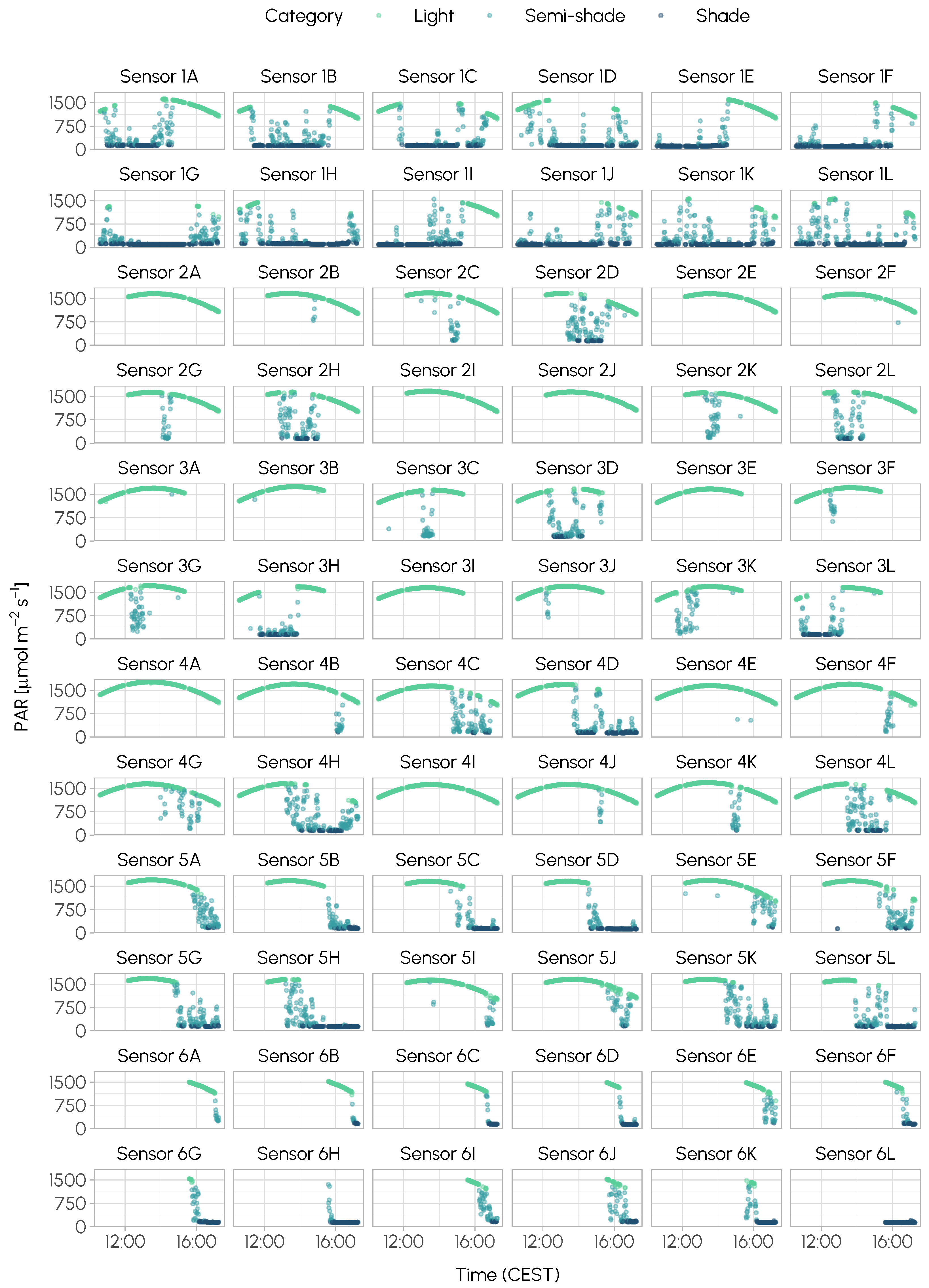
2.2.5. Light Measurements

To validate the simulated shadow with reference data, light measurements were taken under the apple tree using quantum sensors. On 10 August 2023, 60 light sensors were placed on the ground north of the stem base. On that day, the weather was cloudless and there was no rain. From 8:00 to 18:00 CEST, the average diffuse radiation was 30.3 J/cm²/h and the average global radiation was 242.3 J/cm²/h [58]. We used SQ-110 quantum sensors (Apogee Instruments, Logan, UT, USA) and recorded the measurements with Adafruit Feather 32u4 Adalogger data loggers (Adafruit Industries, New York City, NY, USA). These sensors record radiation in a spectral range from 410 nm to 655 nm, corresponding to photosynthetically active radiation (PAR). Each logger was wired to 12 sensors that were mounted to wooden frames (2 m × 3 m) to increase their visibility within the TLS data, to elevate them above the grass sward, and to level them (see Figure 4).

The sensors recorded the incoming light radiation once per minute from 10:35 to 17:15 CEST. During this period, the wooden sensor frames were repositioned twice, between 11:55 and 12:10 CEST and between 15:20 and 15:35 CEST. The data collected by the sensors during these time windows were excluded from the analysis. We repositioned the wooden frames that over time became fully exposed to the Sun, since the goal was to collect data at the edges between light and shade influenced by the tree crown. The sensors were manually georeferenced in CloudCompare using the TLS data. Scanning was only accomplished for two of the three time slots as we initially had issues connecting the TLS device with the GNSS base station. Therefore, not all original frame positions could be reconstructed after the first repositioning event. For this reason, only the data derived from the three frames that remained in situ in the first and second time slot were georeferenced and available for further analysis. For the second and third time slots, data from all five loggers were georeferenced and available for analysis.

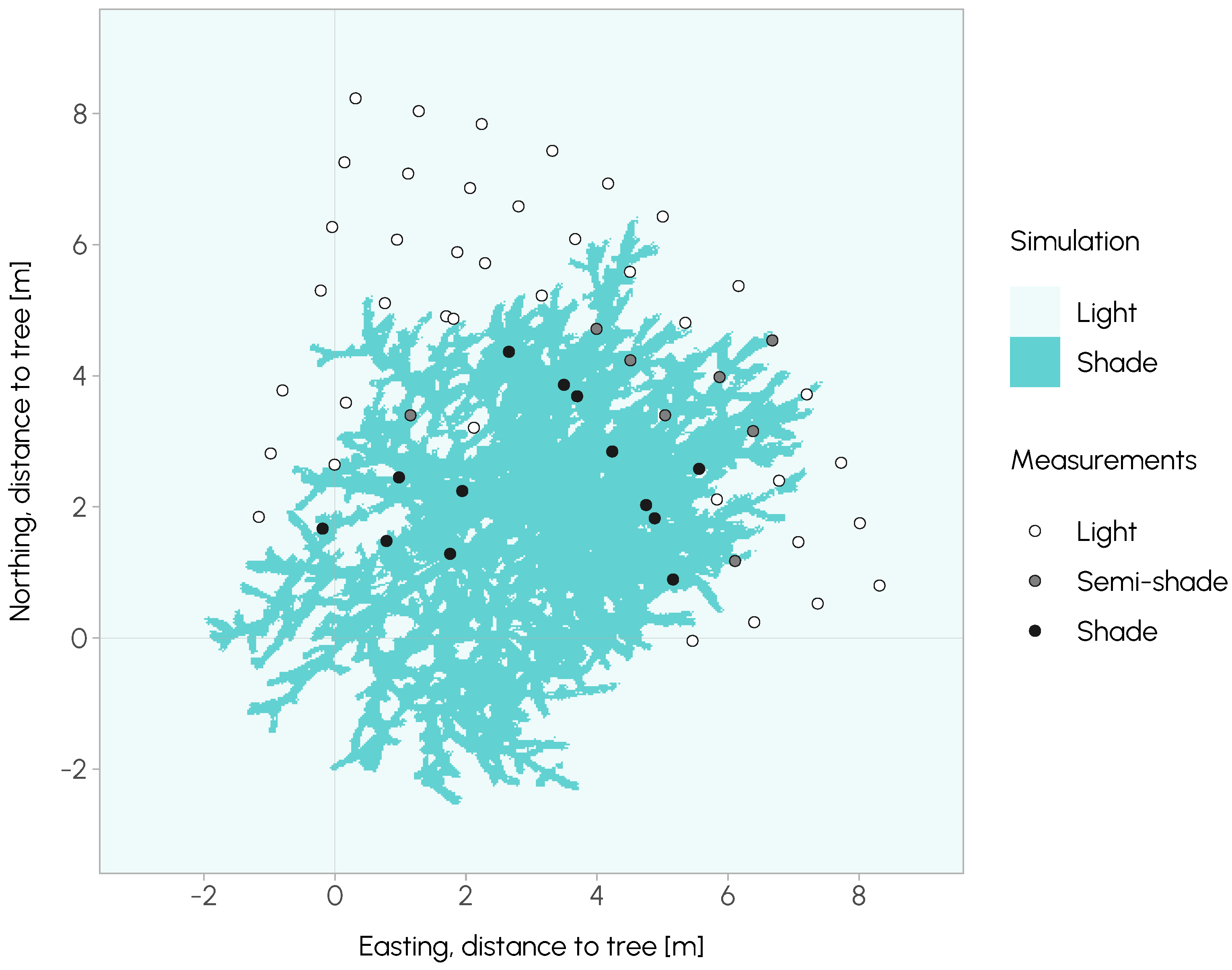
2.2.6. Simulation vs. Measurements

To enable the comparisons between the simulated and measured values that are not affected by the daily radiation pattern, we classified the PAR measurements. The sensors recorded slightly different values, even when positioned under the same light conditions. These small differences are likely due to small differences in their sensitivity and opening angle, as the thin wooden batons were slightly twisted. Therefore, we manually determined thresholds to determine full light or shadow. For each time step i, ${\mathrm{PAR}}_i$ ≥ max(${\mathrm{PAR}}_i$) − 190 µmol ${\mathrm{m}}^{-2}$ ${\mathrm{s}}^{-1}$ was defined as “light”, ${\mathrm{PAR}}_i$ ≤ min(${\mathrm{PAR}}_i$) + 75 µmol ${\mathrm{m}}^{-2}$ ${\mathrm{s}}^{-1}$ was defined as “shade”, and all values in between were defined as “semi-shade”. The classification of each sensor’s measurements is shown in Figure A2. Furthermore, we calculated the relative PAR for each measurement, where 0 = full shade and 1 = full light. The relative PAR was calculated by scaling the values between the minimum and maximum observed PAR values at each time step.

For the simulation, the leaves were simulated based on the manually measured leaf distribution and the leaf size measured from the summer scan. An overview over the simulation parameters is given in Table A1. We simulated the shade for the sampled time frame using a temporal resolution of 1 min and a spatial resolution of 1 cm. We simulated the leaves and the shade for each of the final 25 QSMs. To obtain one final result per time step, we determined whether a cell was shaded or not based on a majority vote, with the most frequent value across all 25 output rasters being the assigned value. From the final output, the values at the sensor locations were extracted (see supplementary materials). Finally, correlations between the simulated and measured values were tested.

2.3. Example Application

To demonstrate the capabilities of our simulation workflow, we simulated leaves and the shade under the study apple tree for one year. According to phenological data from the Deutscher Wetterdienst [58], the bud burst of apple trees in Germany in the years 1996–2016 began on average at the beginning of April, and half of the leaves had fallen by the end of October. Therefore, within our simulation, we assume that apple trees do not bear leaves from November to March. Since we measured the leaf size in August, we assume that we recorded the full leaf length. For the simulation, we assume that the leaves are only half as long in April because they are just starting to grow, and that they have a full leaf length for the remainder of the vegetation period. To account for increasing the leaf density due to new leaf growth, we reduced the leaf density to 75% of full leaf density in April and May. To simulate leaf shedding in autumn, we reduced the leaf density by half in October. For this shade simulation, we chose a temporal resolution of 10 min and a spatial resolution of 10 cm. For each time step, we obtained and averaged the diffuse and global radiation of the last 5 years (2019–2023) from the Deutscher Wetterdienst [58]. Diffuse radiation was assigned to the shaded area and global radiation to the non-shaded area. The results were aggregated once for the whole year and once for the growing season. For this simulation, only one randomly selected QSM was used.

3. Results

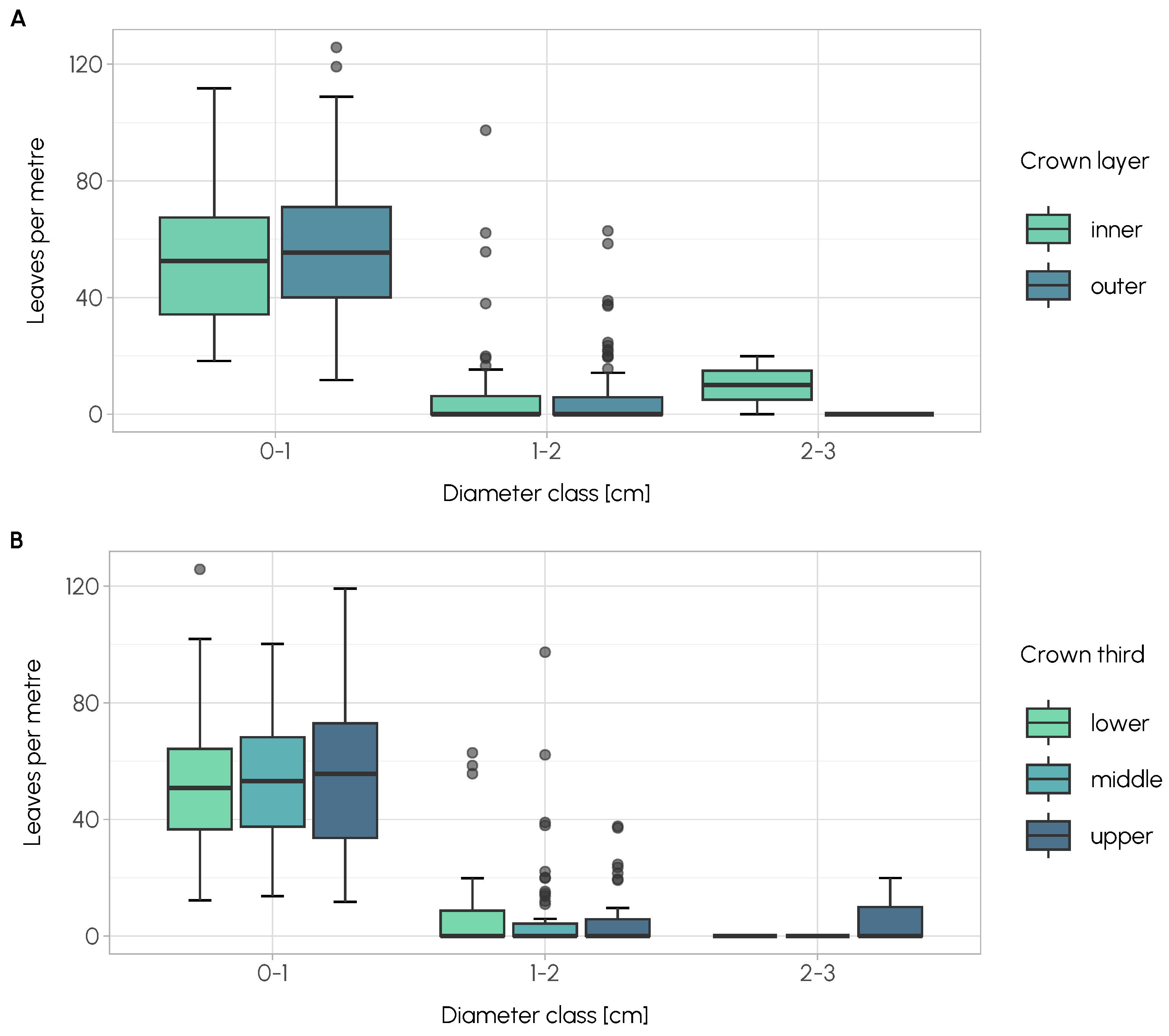
3.1. Leaf Distribution

The results of our manual measurements on the branches show that the leaves were mainly attached to branch segments with a small diameter. As branch diameter increased, the number of leaves per branch length decreased. In the diameter class from 0 cm to 1 cm, there were on average 53.4 leaves/m, in the class from 1 cm to 2 cm, there were 7.6 leaves/m, and in the class from 2 cm to 3 cm there were 4.6 leaves/m. These values are the arithmetic means within the diameter classes, weighted by the sampled length within each class per branch. Data points describing longer branch segments were weighted more heavily.

3.2. Simulation vs. Measurements

The radiation measured by all sensors over the sample period ($n=\mathrm{20,436}$) is shown in Figure 5A. The values between the minimum and maximum measurements resemble a random scatter. However, when inspecting the data from every sensor separately (Figure A2), it becomes evident that the scattering is not randomly distributed. Instead, it shows small-scale changes in light availability, likely caused by the shadows of small branches or sun flecks. The measured radiation pattern is similar to the reference data from the Deutscher Wetterdienst [58]. Full-light measurements resemble the global radiation, and full shadow measurements resemble the diffuse radiation (see Figure 5).

The rasterised simulation output is depicted in Figure 6 for several points in time. As can be seen, we were able to simulate shading at a high temporal and spatial resolution. The high spatial resolution allows us to discern the shadows of individual branches on the ground, as well as small sun flecks between the shadows of outer branches and where the canopy was sparse.

Figure 6 shows both the simulation outputs and corresponding categorised light measurements. In the areas where the simulation predicted full sun, the sensors mostly show corresponding values. In the areas in which shadow was simulated, the sensors predominantly recorded full shade or partial shade. The areas in which semi-shade was measured are located at the edges of the simulated shade and in light patches within the crown shadow (see Figure A3). The simulation and the measurements obtained throughout the entire sampling campaign are compared in Figure 7. As illustrated in the confusion matrix, full light was predicted in the simulation for the large majority of measurements with high radiation (98.33%), and shade was predicted for the majority of low radiation measurements (91.38%). Light measurements of the quantum sensors that were categorised as semi-shade were assigned by our model to either the light (43.03%) or shade category (56.97%), as our model does not contain a corresponding category.

In order to statistically compare the simulation with the measurements, various correlations were calculated using Pearson’s correlation coefficient r. All correlations were found to be significant at $p<0.001$. The correlation between the simulated values (shade: 0, light: 1) and the measured PAR values was $r=0.82$. When using the relative PAR, i.e., the PAR values scaled between the minimum and maximum PAR values per time step, the correlation is slightly stronger at $r=0.84$. Since the aim of our model is to predict full shadow or full light, without semi-shade, we also calculated the correlation between the simulation and the measurements excluding all semi-shade measurements. In this case, the simulation correlates with the measured PAR with a correlation coefficient of $r=0.88$, and with the relative PAR with a correlation coefficient of $r=0.91$.

3.3. Example Application

The results of the shadow simulation for an entire year and for the vegetation period of one year are shown in Figure 8. For both periods, the shadow is located to the north of the tree in the form of an ellipse. The base of the tree trunk is located near the centre of the ellipse. The closer to the centre, the greater the radiation reduction. In the simulation for a whole year, an area of 49.55 m² is subject to a light reduction of at least 10%, 17.74 m² to a light reduction of at least 20% and 0.12 m² to a light reduction of at least 30%. The maximum light reduction is 55% with an area of 0.03 m² directly at the stem base. When simulating the light reduction for the vegetation period only, an area of 57.08 m² experiences at least 10% light reduction, 25.01 m² experiences at least 20% light reduction, 4.34 m² experiences at least 30% light reduction and 0.04 m² experiences at least 40% light reduction. The greatest reduction in light availability observed in this simulation is 57% over an area of 0.03 m² at the stem base.

3.4. Computational Efficiency

For the computation, we used a computer with 128 GB of DDR3-RAM and a 16-core processor (3.40 GHz each). The leaf and shade simulation for the final 25 QSMs over the entire measurement period in a temporal resolution of 1 min, i.e., 401 time steps including the measurement breaks, and a spatial resolution of 1 cm within an area of 375 m² around the tree took about 2.75 h. Thus, on average, the calculation for one QSM took about 7 min. It should be mentioned that most shadow simulation applications probably do not require such a high temporal and spatial resolution. The leaf shade simulation for a single QSM over one year in a temporal resolution of 10 min, i.e., 26,466 time steps excluding night time, and a spatial resolution of 10 cm within an area of 300 m² around the tree took about 3.5 h.

4. Discussion

In this study, we present a shade simulation approach that is based on the 3D data of trees and simulated leaves. To validate the approach, we used a dense and extensive network of 60 quantum sensors and measured the light availability under the tree for one day. Upon validation with the light measurements, we found the simulation to strongly correlate with the measurements ($r\ge 0.82$). Finally, shading under the sample apple tree was simulated over the course of a year. The computation times were considerably reduced compared to a similar previous study. In the following, we discuss the accuracy, advantages, and disadvantages of the approach and illustrate potential applications in the context of AFS.

4.1. Simulation Accuracy

This study demonstrates that it is possible to efficiently simulate leaves and the resultant shade with high accuracy. Our results show good agreement between the light measurements and the shading simulation. From the results, it is evident that the model is very accurate for full light and full shade, but has weaknesses regarding semi-shaded areas. This is underpinned by the different correlations between the measurements and the simulation when including or excluding semi-shade measurements. Caused by the lack of a semi-shade category within our model, this can be attributed to the simulation approach itself. Nevertheless, we are confident that our approach is a good compromise between model accuracy and model complexity. The slight transparency and blurred edges of shadows, i.e., semi-shade, are likely negligible in an area and value when simulating and aggregating across longer time frames, but the absence of such areas becomes evident when simulating radiation at a spatial high resolution for single points in time.

Although we already achieved a high level of predictive power, our model could be further improved by taking the effect of gravity and tree growth into account. In our approach, simulated leaves are placed on a scanned scaffold structure derived from scans taken under leaf-off conditions. However, we expect that branch placement, especially in terms of height, likely varies between leaf-on and leaf-off conditions due to the additional weight of the leaf biomass. Previous studies showed that the ratio of leaf to wood biomass can reach up to 14%, although this varies between tree species [59]. A lowering of total branch angle of wild cherry (Prunus avium L.) was previously measured using TLS over a three-year period [60], here the additional branch weight was due to the branch extension over time, and the same effect can be expected with an increased branch weight due to increased leaf biomass. Wood characteristics such as hardness or bending strength vary depending on various factors [61] and the likely effect of branch reactions to added weight. Therefore, it would be extremely difficult to implement gravity in our model and replicate real branch angles under leaf-on conditions. Furthermore, there is a time lag when simulating shading in another season than that in which the data were collected. If the tree is scanned in the winter before the simulation, it has marginally shorter and thinner branches in the simulation than it would actually have during the simulation period. In a retrospective simulation, as carried out in the validation process, the branches of the QSM are longer and thicker than they would actually be. However, branch growth in terms of length and diameter is hard to predict, since tree growth depends on various factors such as light availability, water supply, temperatures, soil fertility and individual tree management such as pruning [62].

Matching every simulation approach based on remote sensing data, our approach is also limited by the data quality. Currently, TLS is considered to produce the more accurate 3D point clouds of trees compared to other techniques, especially regarding small trees and branches [63,64]. Nevertheless, recent studies have shown the limitations of TLS for capturing small diameter branches, whose diameters are overestimated and the lengths are underestimated [48,49] especially at an increasing distance from the scanner. Due to the small dimension of the tree and the multi-scan approach, we were able to minimise this error source. Still, our approach is susceptible to these effects because the leaves are added and distributed within the branch scaffold based on branch diameters. To circumvent these issues, we shifted the leaf distribution by one diameter class.

Aside from issues inherent to the approach, the calculated accuracy of our simulation is also limited by the validation approach. First of all, we only derived one static set of leaves for each QSM. However, over the course of a day, branches and leaves move due to wind but also due to circadian rhythms, which can alter leaf angles due to variable turgor pressure or as a reaction to solar radiation [65]. Neglecting these movements may have affected our accuracy, but this effect is likely small. Despite this minor uncertainty, our tool can be applied to simulate different leaf sets with different leaf angles for every time step. Furthermore, there is likely some noise in the light measurements. For the validation, we aimed to place the quantum sensors within regions on the ground where we assumed our model would have the most difficulty in making predictions. For all of these reasons, we posit that the actual accuracy of our approach may be slightly superior to that which we estimated.

The accuracy of our approach might also be slightly affected by the unevenness of the ground, the utilisation of 2D leaves and leaf clumping. Leaf spatial distribution has been shown to have a significant effect on the differences in branch-scale light interception [66]. Currently, our approach assumes a flat terrain to maintain computational efficiency. Slope and small undulations are not accounted for within the model. This could have led to small inaccuracies, as the ground below the tree was not perfectly even, thus, skewing the shaded area. To implement a ground texture, the shadow would have to be projected onto a mesh along the direction of the sun, which would require more complex mathematical operations. Furthermore, we implemented leaves as 2D polygons. Although it would be computationally more expensive, 3D leaves may produce more realistic results. This could be part of the reason why we slightly tended to overestimate light. To implement 3D leaves in a way that enables complex leaf shapes containing concave elements, the shape would have to be divided into a number of simple geometries, e.g., triangles, which would have to be projected separately onto the ground. Furthermore, some noise might be explained by leaf clumping. Our approach assumes a homogeneous leaf distribution, but in reality, leaves are often clustered. The implementation of leaf clumping would likely involve some random factors, which could introduce instability into the model.

4.2. Comparison with Other Approaches

Comparison with other shading simulation approaches is hampered by the lack of validation with the real measurements of previous studies [45,46,47]. Validation is often bypassed, as it can be tedious and requires a large number of data points over a large area, in our case, collected using quantum sensors [26]. To enable a fair comparison between different shading models, a large and publicly available benchmark dataset would be required. Although we acquired a large dataset ($n=\mathrm{20,436}$), we assume that an even larger dataset over longer time periods under different environmental conditions, e.g., including individual trees and stands, flat and sloped terrain and different tree species, would be necessary to validate our approach across those conditions.

Similar problems arise when trying to compare the computational efficiency with prior approaches. Most similar previous studies did not report the required computation time [45,47]. One similar study that did reported the time required for computation suggested the simulation of the shade of one QSM of a similar-sized tree, in a spatial and temporal resolution of 10 min and 10 cm, took 16 h to simulate shading for one month without leaves and 52 h for one month with leaves [46]. Assuming the same leaf phenology as we applied, this would result in a total computation time of 444 h for one simulated year. Comparing this with our reported computation time, our approach was faster by a factor of approximately $\times 125$. Even though the simulations might not be completely comparable due to the different number of cylinders in the QSMs and since they rasterised their polygons over a larger area, it is obvious that our code works faster. Both our study and that from Bohn Reckziegel et al. [46] are based on the code from Rosskopf et al. [45]. Here, we were able to increase computational efficiency by vectorising mathematical computations and parallelising the computation.

Compared to other approaches, our approach stands out due to a technically unlimited spatial and temporal resolution. The spatial resolution is factually unlimited since the approach relies on vector data, which can be rasterised to any resolution. The temporal resolution is only limited by the availability of data regarding the sun’s position. Furthermore, in contrast to some other approaches, e.g., approaches based on the turbid medium analogy [67] or on crown ellipsoids with a clumping factor [29], we are able to showcase the heterogeneity of tree shadows in terms of the gaps in the canopy or between outer branches (see Figure A3). In general, the simulation of single leaves likely produces more realistic results than other approaches aggregating leaves [45] or even the whole crown as shapes such as ellipsoids [29]. Another advantage of our method over other approaches is the reduced need for 3D data acquisition. For other approaches that are purely driven by remote sensing data (e.g., [31,32,68]), it is necessary to capture the deciduous trees both under leaf-on and leaf-off conditions if light is to be simulated for a whole year. Our approach provides efficiencies, since once data concerning leaf distribution are available, each target tree only needs to be scanned once without leaves. Therefore, the time and material costs of data acquisition can be reduced.

For our approach, detailed information is required regarding branch diameter and length, leaf size and frequency alongside their distribution between branch diameters. Although they entail their own shortcomings, other approaches that rely on the repeated collection of 2D data do not require such additional information. These parameters are likely affected by an array of environmental conditions. For instance, factors such as water and light availability, air temperature, plant size, and the occurrence of a late-frost can influence leaf size and canopy transparency [69,70,71,72,73]. For this reason, such data might only be transferable to sites where trees experience similar environmental conditions and management. For example, pruning can influence tree growth and health [62,74,75], which in turn might alter leaf distribution and size. Another limitation of our approach is that the light is modelled indirectly by calculating the shadow cast and inferring light availability from radiation data. This requires local solar radiation data, in which the local effects of clouds are already included. However, this limitation probably applies to other light simulations as well. In our case, we recorded the data on a cloudless day.

4.3. Example Application

The basic aim of this study was to utilise 3D remote sensing data for the evaluation of shading caused by trees in AFS. Using our presented approach, it is possible to predict the amount of incoming solar radiation on the ground under trees, which is available to crops planted in an AFS, at any location around a tree at any point in time. In general, light management within the farmed landscape is of high importance, as it may result in reduced yields, dependent on crop, location and the degree and duration of shading [76,77].

Our example application across one year showed that radiation was more strongly decreased within the vegetation period than across the whole year. This is likely caused by the smaller difference between diffuse and global radiation and the denser shade due to the foliage. In a recent meta-analysis, crop-specific meta-regressions as a function of reduced solar radiation were presented as a result of shading and intercropping experiments [77]. Laub et al. [77] modelled increased yields up to a 50% reduction in solar radiation for berries, fruits, and fruity vegetables before yield reductions become evident as shading increases further. Larger reductions in yield were suggested for other crop types such as leafy vegetables, grains, tubers, and legumes from relatively small reductions in incoming solar radiation. Applying this research to our simulation, under the conservative assumption that crops were not planted within a radius of 2 m from the stem, a maximum reduction in solar radiation reached 34% during the vegetation period, and 29% over the whole year. Applying the work of Laub et al. [77] to our simulation, we can suggest that there would be no negative shading effect for fruit and berry crops and only moderate impacts on cereals and grains below our sample apple tree. Furthermore, shading effects are not uniform in all directions as the shade is localised to the north of the tree. As demonstrated, the simulated radiation reduction may be used to estimate shading effects on crop yield.

In our simulation, we used a spatial resolution of 10 cm. Since every grid cell with a shadow polygon below its cell centre is fully categorised as a “shade”, our simulation likely slightly overestimates the shading and, therefore, gives conservative estimates. Furthermore, it should be mentioned that our assumed phenology might not be perfectly accurate for the chosen tree. We utilised aggregated average data derived from a third party [58] as a baseline estimate. However, we acknowledge that there will be variation in phenology due to specific site conditions, topography, and individual tree characteristics [78,79]. To obtain the highest quality shading simulation, the specific phenology of the individually investigated trees could be assessed.

Currently, our tool calculates radiation for single trees, which can be considered one of the smallest building blocks within AFS. In the future, the approach could be enhanced to accommodate groups of trees, hedgerows, or other woody landscape features. By upscaling the approach, it could be incorporated into planning tools that provide decision support at the field or farm level. Such a tool could assist practitioners in early planning stages such as at the time of tree planting. This may include decisions such as tree species choice (in terms of tree size, leaf density, or time of leaf burst alongside defined production goals) as well as their spatial arrangement and density. Equally important aspects to consider are the matching of suitable crops that interact with the tree canopy, i.e., those that display a matching shade tolerance to the induced site conditions. For example, C4 plants are known to react more negatively to shading than C3 plants, which can sometimes benefit from increased shading [15]. Furthermore, essential management activities such as the pruning of primary branches for the production of valuable timber can be more effectively planned to influence shading intensity [80] and can moreover be targeted for maximum or minimum impact on a crop at selected times of the year.

5. Conclusions

In this paper, we present and validate a shade simulation approach based on TLS data and leaf simulations on tree structure models. The validation using a dense network of quantum sensors showed good agreement between measured and simulated light. Our approach enables simulations at extremely high spatial and temporal resolutions and offers improved computational efficiency compared to previous models. Since the leaves are simulated, TLS data must only be collected once during winter dormancy, increasing efficiency and decreasing cost. This work further demonstrates the versatility of TLS and QSMs beyond the sole modelling of 3D structures.

Future research could use our model to investigate tree shading in agricultural landscapes, e.g., to estimate yield changes or to optimise the spatial arrangement of AFS to minimise or maximise shading. Although our approach has demonstrated many advantages, it has some limitations that highlight possible future developments. Future improvements could include the use of 3D leaf shapes instead of 2D leaf polygons. Implementing sloped and uneven terrain using digital terrain models could also improve the simulations and is a challenging but logical next step. In addition, accounting for downward branch movement or growth over multiple seasons could further improve the accuracy of the simulations. Expanding the model to include larger tree sizes and more tree species could also be a priority. However, although there is room for improvement, we consider the simulation approach in its current state an efficient compromise between model accuracy and model complexity.

References

1. Blackman, G.E.; Black, J.N. Physiological and ecological studies in the analysis of plant environment. Ann. Bot. 1959, 23, 131–145. [Google Scholar] [CrossRef]
2. Lupi, C.; Morin, H.; Deslauriers, A.; Rossi, S. Xylem phenology and wood production: Resolving the chicken-or-egg dilemma. Plant Cell Environ. 2010, 33, 1721–1730. [Google Scholar] [CrossRef] [PubMed]
3. Kothari, S.; Montgomery, R.A.; Cavender-Bares, J. Physiological responses to light explain competition and facilitation in a tree diversity experiment. J. Ecol. 2021, 109, 2000–2018. [Google Scholar] [CrossRef]
4. Leuchner, M.; Hertel, C.; Rötzer, T.; Seifert, T.; Weigt, R.; Werner, H.; Menzel, A. Solar radiation as a driver for growth and competition in forest stands. In Growth and Defence in Plants; Ecological Studies; Matyssek, R., Schnyder, H., Osswald, W.F., Ernst, D., Munch, J.C., Pretzsch, H., Eds.; Springer: Berlin/Heidelberg, Germany, 2012; Volume 220, pp. 175–191. [Google Scholar] [CrossRef]
5. Ptushenko, O.S.; Ptushenko, V.V.; Solovchenko, A.E. Spectrum of light as a determinant of plant functioning: A historical perspective. Life 2020, 10, 25. [Google Scholar] [CrossRef] [PubMed]
6. Friedel, A.; von Oheimb, G.; Dengler, J.; Härdtle, W. Species diversity and species composition of epiphytic bryophytes and lichens–A comparison of managed and unmanaged beech forests in NE Germany. Feddes Repert. 2006, 117, 172–185. [Google Scholar] [CrossRef]
7. Sagar, R.; Singh, A.; Singh, J.S. Differential effect of woody plant canopies on species composition and diversity of ground vegetation: A case study. Trop. Ecol. 2008, 49, 189. [Google Scholar]
8. Fu, P.; Rich, P.M. A geometric solar radiation model with applications in agriculture and forestry. Comput. Electron. Agric. 2002, 37, 25–35. [Google Scholar] [CrossRef]
9. Zellweger, F.; de Frenne, P.; Lenoir, J.; Rocchini, D.; Coomes, D. Advances in microclimate ecology arising from remote sensing. Trends Ecol. Evol. 2019, 34, 327–341. [Google Scholar] [CrossRef] [PubMed]
10. Helbach, J.; Frey, J.; Messier, C.; Mörsdorf, M.; Scherer-Lorenzen, M. Light heterogeneity affects understory plant species richness in temperate forests supporting the heterogeneity-diversity hypothesis. Ecol. Evol. 2022, 12, e8534. [Google Scholar] [CrossRef]
11. Way, D.A.; Pearcy, R.W. Sunflecks in trees and forests: From photosynthetic physiology to global change biology. Tree Physiol. 2012, 32, 1066–1081. [Google Scholar] [CrossRef]
12. Nair, P.K.R.; Kumar, B.M.; Nair, V.D. Definition and concepts of agroforestry. In An Introduction to Agroforestry; Springer International Publishing: Cham, Switzerland, 2021; pp. 21–28. [Google Scholar] [CrossRef]
13. Dufour, L.; Metay, A.; Talbot, G.; Dupraz, C. Assessing light competition for cereal production in temperate agroforestry systems using experimentation and crop modelling. J. Agron. Crop. Sci. 2013, 199, 217–227. [Google Scholar] [CrossRef]
14. Ehret, M.; Graß, R.; Wachendorf, M. The effect of shade and shade material on white clover/perennial ryegrass mixtures for temperate agroforestry systems. Agrofor. Syst. 2015, 89, 557–570. [Google Scholar] [CrossRef]
15. Lin, C.; McGraw, R.; George, M.; Garrett, H. Shade effects on forage crops with potential in temperate agroforestry practices. Agrofor. Syst. 1998, 44, 109–119. [Google Scholar] [CrossRef]
16. Somporn, C.; Kamtuo, A.; Theerakulpisut, P.; Siriamornpun, S. Effect of shading on yield, sugar content, phenolic acids and antioxidant property of coffee beans (Coffea arabica L. cv. Catimor) harvested from north-eastern Thailand. J. Sci. Food Agric. 2012, 92, 1956–1963. [Google Scholar] [CrossRef] [PubMed]
17. Kohli, R.K.; Singh, H.P.; Batish, D.R.; Jose, S. Ecological interactions in agroforestry: An overview. In Ecological Basis of Agroforestry; CRC Press: Boca Raton, FL, USA, 2008; pp. 3–14. [Google Scholar]
18. Valtorta, S.E.; Leva, P.E.; Gallardo, M.R. Evaluation of different shades to improve dairy cattle well-being in Argentina. Int. J. Biometeorol. 1997, 41, 65–67. [Google Scholar] [CrossRef] [PubMed]
19. Mancera, K.F.; Zarza, H.; de Buen, L.L.; García, A.A.C.; Palacios, F.M.; Galindo, F. Integrating links between tree coverage and cattle welfare in silvopastoral systems evaluation. Agron. Sustain. Dev. 2018, 38, 19. [Google Scholar] [CrossRef]
20. Pezzopane, J.R.M.; Nicodemo, M.L.F.; Bosi, C.; Garcia, A.R.; Lulu, J. Animal thermal comfort indexes in silvopastoral systems with different tree arrangements. J. Therm. Biol. 2019, 79, 103–111. [Google Scholar] [CrossRef] [PubMed]
21. Tsonkova, P.; Mirck, J.; Böhm, C.; Fütz, B. Addressing farmer-perceptions and legal constraints to promote agroforestry in Germany. Agrofor. Syst. 2018, 92, 1091–1103. [Google Scholar] [CrossRef]
22. Evans, G.C.; Coombe, D.E. Hemisperical and woodland canopy photography and the light climate. J. Ecol. 1959, 47, 103–113. [Google Scholar] [CrossRef]
23. Hale, S.E.; Edwards, C. Comparison of film and digital hemispherical photography across a wide range of canopy densities. Agric. For. Meteorol. 2002, 112, 51–56. [Google Scholar] [CrossRef]
24. Ferment, A.; Picard, N.; Gourlet-Fleury, S.; Baraloto, C. A comparison of five indirect methods for characterizing the light environment in a tropical forest. Ann. For. Sci. 2001, 58, 877–891. [Google Scholar] [CrossRef]
25. Yan, G.; Hu, R.; Luo, J.; Weiss, M.; Jiang, H.; Mu, X.; Xie, D.; Zhang, W. Review of indirect optical measurements of leaf area index: Recent advances, challenges, and perspectives. Agric. For. Meteorol. 2019, 265, 390–411. [Google Scholar] [CrossRef]
26. Engelbrecht, B.M.J.; Herz, H.M. Evaluation of different methods to estimate understorey light conditions in tropical forests. J. Trop. Ecol. 2001, 17, 207–224. [Google Scholar] [CrossRef]
27. Reid, R.; Ferguson, I.S. Development and validation of a simple approach to modelling tree shading in agroforestry systems. Agrofor. Syst. 1992, 20, 243–252. [Google Scholar] [CrossRef]
28. Dupraz, C.; Liagre, F. Agroforesterie: Des Arbres et des Cultures, 2nd ed.; Éditions France Agricole: Paris, France, 2011. [Google Scholar]
29. Talbot, G.; Dupraz, C. Simple models for light competition within agroforestry discontinuous tree stands: Are leaf clumpiness and light interception by woody parts relevant factors? Agrofor. Syst. 2012, 84, 101–116. [Google Scholar] [CrossRef]
30. Somarriba, E.; Zamora, R.; Barrantes, J.; Sinclair, F.L.; Quesada, F. ShadeMotion: Tree shade patterns in coffee and cocoa agroforestry systems. Agrofor. Syst. 2023, 97, 31–44. [Google Scholar] [CrossRef]
31. Bittner, S.; Gayler, S.; Biernath, C.; Winkler, J.B.; Seifert, S.; Pretzsch, H.; Priesack, E. Evaluation of a ray-tracing canopy light model based on terrestrial laser scans. Can. J. Remote. Sens. 2012, 38, 619–628. [Google Scholar] [CrossRef]
32. Li, W.; Guo, Q.; Tao, S.; Su, Y. VBRT: A novel voxel-based radiative transfer model for heterogeneous three-dimensional forest scenes. Remote. Sens. Environ. 2018, 206, 318–335. [Google Scholar] [CrossRef]
33. Roupsard, O.; Dauzat, J.; Nouvellon, Y.; Deveau, A.; Feintrenie, L.; Saint-André, L.; Mialet-Serra, I.; Braconnier, S.; Bonnefond, J.M.; Berbigier, P.; et al. Cross-validating sun-shade and 3D models of light absorption by a tree-crop canopy. Agric. For. Meteorol. 2008, 148, 549–564. [Google Scholar] [CrossRef]
34. Dassot, M.; Constant, T.; Fournier, M. The use of terrestrial LiDAR technology in forest science: Application fields, benefits and challenges. Ann. For. Sci. 2011, 68, 959–974. [Google Scholar] [CrossRef]
35. Calders, K.; Adams, J.; Armston, J.; Bartholomeus, H.; Bauwens, S.; Bentley, L.P.; Chave, J.; Danson, F.M.; Demol, M.; Disney, M.; et al. Terrestrial laser scanning in forest ecology: Expanding the horizon. Remote Sens. Environ. 2020, 251, 112102. [Google Scholar] [CrossRef]
36. Schindler, Z.; Morhart, C.; Sheppard, J.P.; Frey, J.; Seifert, T. In a nutshell: Exploring single tree parameters and above-ground carbon sequestration potential of common walnut (Juglans regia L.) in agroforestry systems. Agrofor. Syst. 2023, 97, 1007–1024. [Google Scholar] [CrossRef]
37. Schindler, Z.; Seifert, T.; Sheppard, J.P.; Morhart, C. Allometric models for above-ground biomass, carbon and nutrient content of wild cherry (Prunus avium L.) trees in agroforestry systems. Ann. For. Sci. 2023, 80, 28. [Google Scholar] [CrossRef]
38. Liang, X.; Kankare, V.; Hyyppä, J.; Wang, Y.; Kukko, A.; Haggrén, H.; Yu, X.; Kaartinen, H.; Jaakkola, A.; Guan, F.; et al. Terrestrial laser scanning in forest inventories. ISPRS J. Photogramm. Remote. Sens. 2016, 115, 63–77. [Google Scholar] [CrossRef]
39. Malhi, Y.; Jackson, T.; Bentley, L.P.; Lau, A.; Shenkin, A.; Herold, M.; Calders, K.; Bartholomeus, H.; Disney, M.I. New perspectives on the ecology of tree structure and tree communities through terrestrial laser scanning. Interface Focus 2018, 8, 20170052. [Google Scholar] [CrossRef] [PubMed]
40. Lumme, J.; Karjalainen, M.; Kaartinen, H.; Kukko, A.; Hyyppä, J.; Hyyppä, H.; Jaakkola, A.; Kleemola, J. Terrestrial laser scanning of agricultural crops. Int. Arch. Photogramm. Remote. Sens. Spat. Inf. Sci. 2008, XXXVII, 563–566. [Google Scholar]
41. Tamás, J.; Riczu, P.; Nagy, G.; Nagy, A.; Jancsó, T.; Nyéki, J.; Szabó, Z. Applicability of 3D laser scanning in precision horticulture. Int. J. Hortic. Sci. 2011, 17, 55–58. [Google Scholar] [CrossRef]
42. Wu, D.; Johansen, K.; Phinn, S.; Robson, A. Suitability of airborne and terrestrial laser scanning for mapping tree crop structural metrics for improved orchard management. Remote Sens. 2020, 12, 1647. [Google Scholar] [CrossRef]
43. Kunz, M.; Hess, C.; Raumonen, P.; Bienert, A.; Hackenberg, J.; Maas, H.G.; Härdtle, W.; Fichtner, A.; von Oheimb, G. Comparison of wood volume estimates of young trees from terrestrial laser scan data. iForest-Biogeosci. For. 2017, 10, 451–458. [Google Scholar] [CrossRef]
44. Raumonen, P.; Åkerblom, M. InverseTampere/TreeQSM, Version 2.4.1; Zenodo: Geneva, Switzerland, 2022. [Google Scholar] [CrossRef]
45. Rosskopf, E.; Morhart, C.; Nahm, M. Modelling shadow using 3D tree models in high spatial and temporal resolution. Remote Sens. 2017, 9, 719. [Google Scholar] [CrossRef]
46. Bohn Reckziegel, R.; Larysch, E.; Sheppard, J.P.; Kahle, H.P.; Morhart, C. Modelling and comparing shading effects of 3D tree structures with virtual leaves. Remote Sens. 2021, 13, 532. [Google Scholar] [CrossRef]
47. Calders, K.; Origo, N.; Burt, A.; Disney, M.; Nightingale, J.; Raumonen, P.; Åkerblom, M.; Malhi, Y.; Lewis, P. Realistic forest stand reconstruction from terrestrial LiDAR for radiative transfer modelling. Remote Sens. 2018, 10, 933. [Google Scholar] [CrossRef]
48. Demol, M.; Wilkes, P.; Raumonen, P.; Krishna Moorthy, S.M.; Calders, K.; Gielen, B.; Verbeeck, H. Volumetric overestimation of small branches in 3D reconstructions of Fraxinus excelsior. Silva Fenn. 2022, 56, 10550. [Google Scholar] [CrossRef]
49. Morhart, C.; Schindler, Z.; Frey, J.; Sheppard, J.P.; Calders, K.; Disney, M.; Morsdorf, F.; Raumonen, P.; Seifert, T. Limitations of estimating branch volume from terrestrial laser scanning. Eur. J. For. Res. 2024, 143, 687–702. [Google Scholar] [CrossRef]
50. Raumonen, P.; Kaasalainen, M.; Åkerblom, M.; Kaasalainen, S.; Kaartinen, H.; Vastaranta, M.; Holopainen, M.; Disney, M.; Lewis, P. Fast automatic precision tree models from terrestrial laser scanner data. Remote Sens. 2013, 5, 491–520. [Google Scholar] [CrossRef]
51. Calders, K.; Newnham, G.; Burt, A.; Murphy, S.; Raumonen, P.; Herold, M.; Culvenor, D.; Avitabile, V.; Disney, M.; Armston, J. Nondestructive estimates of above-ground biomass using terrestrial laser scanning. Methods Ecol. Evol. 2015, 6, 198–208. [Google Scholar] [CrossRef]
52. Gonzalez de Tanago, J.; Lau, A.; Bartholomeus, H.; Herold, M.; Avitabile, V.; Raumonen, P.; Martius, C.; Goodman, R.C.; Disney, M.; Manuri, S.; et al. Estimation of above-ground biomass of large tropical trees with terrestrial LiDAR. Methods Ecol. Evol. 2018, 9, 223–234. [Google Scholar] [CrossRef]
53. R Core Team. R: A Language and Environment for Statistical Computing. Available online: https://www.R-project.org/ (accessed on 23 May 2024).
54. Schindler, Z. qsm2r: Import and Analyze QSMs from TreeQSM in R. Available online: https://github.com/zoeschindler/qsm2r (accessed on 23 May 2024).
55. Schindler, Z. qsm2shade: Analyze shade cast of QSMs. Available online: https://github.com/zoeschindler/qsm2shade (accessed on 23 May 2024).
56. Hijmans, R.J. Terra: Spatial Data Analysis, R Package Version 1.7-39; R Core Team: Vienna, Austria, 2023. [Google Scholar]
57. Peel, M.C.; Finlayson, B.L.; McMahon, T.A. Updated world map of the Köppen-Geiger climate classification. Hydrol. Earth Syst. Sci. 2007, 4, 439–473. [Google Scholar] [CrossRef]
58. Deutscher Wetterdienst. Climate Data Center. Available online: https://www.dwd.de/EN/climate_environment/cdc/cdc_en.html (accessed on 17 April 2024).
59. Mensah, S.; Glèlè Kakaï, R.; Seifert, T. Patterns of biomass allocation between foliage and woody structure: The effects of tree size and specific functional traits. Ann. For. Res. 2014, 59, 49–60. [Google Scholar] [CrossRef]
60. Sheppard, J.; Morhart, C.; Hackenberg, J.; Spiecker, H. Terrestrial laser scanning as a tool for assessing tree growth. iFor. Biogeosci. For. 2017, 10, 172–179. [Google Scholar] [CrossRef]
61. Zhu, J.; Shi, Y.; Fang, L.; Liu, X.; Ji, C. Patterns and determinants of wood physical and mechanical properties across major tree species in China. Sci. China Life Sci. 2015, 58, 602–612. [Google Scholar] [CrossRef] [PubMed]
62. Kozlowski, T.T.; Pallardy, S.G. Growth Control in Woody Plants; Physiological Ecology Series; Academic Press: San Diego, CA, USA, 1997. [Google Scholar]
63. Bienert, A.; Georgi, L.; Kunz, M.; Maas, H.G.; von Oheimb, G. Comparison and combination of mobile and terrestrial laser scanning for natural forest inventories. Forests 2018, 9, 395. [Google Scholar] [CrossRef]
64. Brede, B.; Calders, K.; Lau, A.; Raumonen, P.; Bartholomeus, H.M.; Herold, M.; Kooistra, L. Non-destructive tree volume estimation through quantitative structure modelling: Comparing UAV laser scanning with terrestrial LiDAR. Remote Sens. Environ. 2019, 233, 111355. [Google Scholar] [CrossRef]
65. Lüttge, U.; Hertel, B. Diurnal and annual rhythms in trees. Trees Struct. Funct. 2009, 23, 683–700. [Google Scholar] [CrossRef]
66. Massonnet, C.; Regnard, J.L.; Lauri, P.E.; Costes, E.; Sinoquet, H. Contributions of foliage distribution and leaf functions to light interception, transpiration and photosynthetic capacities in two apple cultivars at branch and tree scales. Tree Physiol. 2008, 28, 665–678. [Google Scholar] [CrossRef] [PubMed]
67. Meloni, S.; Sinoquet, H. Assessment of the spatial distribution of light transmitted below young trees in an agroforestry system. Ann. For. Sci. 1997, 54, 313–333. [Google Scholar] [CrossRef]
68. Van der Zande, D.; Stuckens, J.; Verstraeten, W.W.; Muys, B.; Coppin, P. Assessment of light environment variability in broadleaved forest canopies using terrestrial laser scanning. Remote Sens. 2010, 2, 1564–1574. [Google Scholar] [CrossRef]
69. Parkhurst, D.F.; Loucks, O.L. Optimal leaf size in relation to environment. J. Ecol. 1972, 60, 505. [Google Scholar] [CrossRef]
70. St. Clair, S.B.; Monson, S.D.; Smith, E.A.; Cahill, D.G.; Calder, W.J. Altered leaf morphology, leaf resource dilution and defense chemistry induction in frost-defoliated aspen (Populus tremuloides). Tree Physiol. 2009, 29, 1259–1268. [Google Scholar] [CrossRef]
71. Xu, F.; Guo, W.; Xu, W.; Wei, Y.; Wang, R. Leaf morphology correlates with water and light availability: What consequences for simple and compound leaves? Prog. Nat. Sci. 2009, 19, 1789–1798. [Google Scholar] [CrossRef]
72. Wright, I.J.; Dong, N.; Maire, V.; Prentice, I.C.; Westoby, M.; Díaz, S.; Gallagher, R.V.; Jacobs, B.F.; Kooyman, R.; Law, E.A.; et al. Global climatic drivers of leaf size. Science 2017, 357, 917–921. [Google Scholar] [CrossRef] [PubMed]
73. Baumgarten, F.; Gessler, A.; Vitasse, Y. No risk—No fun: Penalty and recovery from spring frost damage in deciduous temperate trees. Funct. Ecol. 2023, 37, 648–663. [Google Scholar] [CrossRef]
74. Hevia, A.; Álvarez-González, J.G.; Majada, J. Comparison of pruning effects on tree growth, productivity and dominance of two major timber conifer species. For. Ecol. Manag. 2016, 374, 82–92. [Google Scholar] [CrossRef]
75. Burgess, T.I.; Howard, K.; Steel, E.; Barbour, E.L. To prune or not to prune; pruning induced decay in tropical sandalwood. For. Ecol. Manag. 2018, 430, 204–218. [Google Scholar] [CrossRef]
76. Sheppard, J.P.; Bohn Reckziegel, R.; Borrass, L.; Chirwa, P.W.; Cuaranhua, C.J.; Hassler, S.K.; Hoffmeister, S.; Kestel, F.; Maier, R.; Mälicke, M.; et al. Agroforestry: An appropriate and sustainable response to a changing climate in Southern Africa? Sustainability 2020, 12, 6796. [Google Scholar] [CrossRef]
77. Laub, M.; Pataczek, L.; Feuerbacher, A.; Zikeli, S.; Högy, P. Contrasting yield responses at varying levels of shade suggest different suitability of crops for dual land-use systems: A meta-analysis. Agron. Sustain. Dev. 2022, 42, 51. [Google Scholar] [CrossRef]
78. Rousi, M.; Pusenius, J. Variations in phenology and growth of European white birch (Betula pendula) clones. Tree Physiol. 2005, 25, 201–210. [Google Scholar] [CrossRef] [PubMed]
79. Bamba, H.; Korbo, A.; Sanou, H.; Ræbild, A.; Kjær, E.D.; Hansen, J.K. Genetic differentiation in leaf phenology among natural populations of Adansonia digitata L. follows climatic clines. Glob. Ecol. Conserv. 2019, 17, e00544. [Google Scholar] [CrossRef]
80. Bohn Reckziegel, R.; Sheppard, J.P.; Kahle, H.P.; Larysch, E.; Spiecker, H.; Seifert, T.; Morhart, C. Virtual pruning of 3D trees as a tool for managing shading effects in agroforestry systems. Agrofor. Syst. 2022, 96, 89–104. [Google Scholar] [CrossRef]
Figure 1. Overview of the general workflow for modelling leaves and shadows. (A) shows the data acquisition using TLS and the pre-processing of the data in RiSCAN PRO. (B) shows the derivation of QSMs using TreeQSM. (C) shows the derivation of the leaf distribution from field data. (D) shows how the leaves and the shade are simulated.
Remotesensing 16 02189 g001
Figure 2. Point clouds of the tree scanned in August 2023 (summer scan, left) and in February 2024 (winter scan, right). The colours of the points indicate the height above the ground.
Remotesensing 16 02189 g002
Figure 3. QSM of the tree scanned in winter mode, with simulated shade (left) and with simulated leaves and shade (right).
Remotesensing 16 02189 g003
Figure 4. Overview of the validation setup. (A) Location of Freiburg im Breisgau within Germany (dark turquoise) in the state of Baden-Württemberg (light turquoise). (B) Photo of the survey setup. (C) Top-view on the tree, with brighter colours indicating larger height. The rectangles are the wooden frames with mounted quantum sensors (dots and diamonds). The dark pink dots are sensors that measured in the same position all day, while the light pink diamonds are sensors that were repositioned.
Remotesensing 16 02189 g004
Figure 5. Radiation during the validation period. (A) Radiation measured using the quantum sensors, with colours indicating the respective logger. Logger 6 is the repositioned logger 3. (B) Reference radiation data from the Deutscher Wetterdienst [58], coloured according to the type of radiation (diffuse, direct, global).
Remotesensing 16 02189 g005
Figure 6. Simulation and measurement of the radiation under the apple tree at different points in time. The dark turquoise area indicates simulated shade, while the light area indicates simulated light. The dots indicate the positions of the quantum sensors. Depending on the brightness of the dots, the sensors recorded full light (light grey), semi-shade (dark grey) or full shade (black). The stem base is placed at ( 0 | 0 ) .
Remotesensing 16 02189 g006
Figure 7. Confusion matrix of the reference data measured with the quantum sensors and the predicted categories based on our model. The category “semi-shade” refers to measurements between full shade and full light. The colours refer to the fraction of the reference class that was correctly classified.
Remotesensing 16 02189 g007
Figure 8. Simulation of the radiation under the apple tree for a whole year or the vegetation period only. Colours indicate the level of light reduction below the tree, compared to open land conditions. The stem base is placed at ( 0 | 0 ) . The black outline shows the outline of the crown projection area.
Remotesensing 16 02189 g008
Disclaimer/Publisher’s Note: The statements, opinions and data contained in all publications are solely those of the individual author(s) and contributor(s) and not of MDPI and/or the editor(s). MDPI and/or the editor(s) disclaim responsibility for any injury to people or property resulting from any ideas, methods, instructions or products referred to in the content.