Self-Calibration Strip Bundle Adjustment of High-Resolution Satellite Imagery

Abstract

The attitude accuracy of high-resolution satellite images is the main factor affecting their geometric positioning accuracy. Bundle block adjustment is the main method for realizing the simultaneous estimation of attitude models for overlapping images over a large area. In the current research on the joint positioning of high-resolution multi-line array satellite images, the adjustment is usually carried out with the view or load as a unit without considering the consistency of the error of the same platform. In this paper, we develop a self-calibration strip bundle adjustment scheme that considers the boresight misalignment among multiple cameras. By introducing the installation angle between multiple loads, we fully utilized their geometric constraint relationship with the same platform to establish a unified attitude compensation model for multiple loads. The experimental results of the ZiYuan3 (ZY-3) satellite image show that, when the ground control points (GCPs) are laid only at four corner points of the image, the image plane and elevation accuracies are 1.85 m and 1.87 m after an adjustment using this method, which can achieve comparable accuracies with those obtained by a traditional program based on an adjustment with more GCPs.

1. Introduction

Current high-resolution optical remote sensing satellites mostly adopt a linear array charge-coupled device (CCD) push-broom scanning imaging method for Earth observation images [1]. Because of the formation of a certain angle in the orbital direction of its multiple line arrays, high-resolution multi-line array satellites can acquire stereo data in the same orbit, which play an important role in Earth observation and deep space [2,3,4,5,6].

The high-accuracy geometric positioning of high-resolution satellite images is the basis for the geometric processing of remote sensing images, obtaining high-accuracy georeferenced information, and the basic guarantee for measuring and producing topographic maps of various scales. Benefiting from the development of high-accuracy orbit determination, attitude determination, and geometric calibration technologies, the current highest-accuracy civil agile satellites, WorldView-3 [7] and Pleiades-1B [8], can be directly positioned within 4 m of the plane (Circular Error 90%, CE90). The factors that have a direct impact on the satellite positioning accuracy are the orbit accuracy and attitude determination accuracy. Because the orbit determination accuracy can be above the sub-meter level [9,10] and the orbit errors can usually be equated to the attitude angle errors [11], the effect of the orbit errors on the geometric positioning accuracy of the images can be ignored. While remote sensing satellites have high flight altitudes, a small attitude error will bring a large ground offset. Therefore, the positioning accuracy of satellite images puts forward high requirements for the accuracy of satellite attitude determination.

Bundle block adjustment is the main method for realizing the simultaneous estimation of attitude models for overlapping images over a large area to improve image accuracy. There are two main modes for the block adjustment of high-resolution satellite images: the direct estimation of the attitude model based on control points, and the estimation of the attitude compensation model. In the early stage, when the accuracy of the attitude measurement was not high, the mainstream method was to take the attitude and orbit measurements as the initial values and estimate them using ground control points (GCPs) based on the assumption of the attitude model. Since Hofmann et al. developed the principle of a three-line-array stereo imaging and an orientation image interpolation model in 1984 [12], block adjustment based on orientation points has become one of the main methods for three-line-array image orientation. Wang developed a linear matrix CCD (LMCCD) camera design based on a three-line array CCD camera with two small CCD matrix arrays on each side of the nadir (NAD) array, which were used to capture the center projection image of the tie points (TPs) of the aerial triangular lock [13]. An equivalent frame photo (EFP) orientation image block adjustment method for the LMCCD camera was presented and applied to the design and practice of the Tianhui-1 (TH-1) satellite [14]. Ebner et al. found that the orbit-constrained adjustment approach solves for fewer parameters and has a better accuracy than the orientation point adjustment approach in MOMS satellite engineering [15]. Poli presented a piecewise polynomial model (PPM) based on orientation points for attitude and orbit modeling [16]. With the continuous development of attitude and orbit determination technologies, the accuracy of attitude and orbit measurements has been increasing. The adjustment method for estimating the attitude and orbit compensation model has the advantages of a high positioning accuracy [17], fewer control points needed [18], and the ability to realize the modeling of attitude jitter [19]; therefore, it is widely used in high-resolution line push-broom satellites. Radhadevi et al. developed generalized polynomial models for modeling sensor positions and attitudes and used them for the adjustment of the Cartosat-1 and Cartosat-2 satellite imagery based on rigorous sensor models [20]. Rottensteiner et al. performed the adjustment with the strip as a unit and reduced the number of GCPs required for the accurate georeferencing of Advanced Land Observation Satellite (ALOS) images by as much as 90%, with an accuracy of better than 1 pixel [21]. Di et al. presented a self-calibration bundle adjustment method by introducing an additional interior orientation parameter into the traditional beam method bundle adjustment model, effectively eliminating the inconsistency between the Chang’E-2 CCD images [22]. Zhang et al. used a quadratic polynomial, systematic error compensation, and orientation image models to conduct adjustment experiments on the three-line array ultra-long orbit images of the TH-1 satellite and analyzed the accuracy levels achieved by different models [23]. Zheng et al. introduced different aberration models to perform the self-calibration bundle adjustment on long-strip images of the China and Brazil Earth Resource Satellite 02B (CBERS-02B), which effectively improved the geometric accuracy of the images [24]. Cao et al. presented a high-resolution satellite image sensor location method based on strip constraints that can simultaneously solve the bias compensation parameters of each standard scene image in a strip with sparse GCPs [25].

The ZiYuan3 (ZY-3) Series 01 satellite was China’s first civilian high-resolution stereo mapping satellite, independently designed and launched on 9 January 2012. The ZY-3 satellite is equipped with a three-line array camera with a forward (FWD) and backward (BWD) view resolution of 3.5 m, a NAD view resolution of 2.1 m, and a multispectral camera with a resolution of 5.8 m [26]. The ZY-3 satellite uses three-line array imaging to acquire the same orbital stereo image and has a side-swing ability to acquire cross-track stereo images. Owing to changes in the thermal environment of space when a high-resolution multi-line array satellite is in orbit, the installation relationship between the multi-line array camera and the star sensitizer carried on the star changes dynamically, resulting in an attitude error that changes in space and time, which has become the key factor restricting the high-accuracy direct positioning of high-resolution multi-line array satellites. The roll angle error introduces an offset in the scanning direction of the image, the pitch angle error introduces an offset in the flight direction [27], and the yaw angle introduces offsets in both the scanning and flight directions. Zhang et al. used 19 strip images for the in-orbit calibration of ZY-3 and introduced a systematic error compensation model to compensate for the position and attitude errors. After the adjustment based on high-accuracy control points, the image plane positioning accuracy and elevation positioning accuracy are 1.3 m and 1.7 m, respectively [28]. Zhang et al. used an attitude offset model for each orbit image to perform the adjustment of ZY-3 long-strip data; the image square residuals were more than one image element [29]. The linear compensation model yielded better results when considering the drift characteristics of low-frequency attitude errors. The ZY-3 satellite image with a length of 560 km can achieve sub-pixel level positioning based on the attitude linear model [30]. In some instances, higher-order models are required [31]. Cao et al. used cubic splines to compensate for the nonlinear deviation caused by the attitude jitter of ZY-3 without ground control points, where the spline coefficients were obtained from the residual estimation of the virtual control points [32].

Owing to the differences in the camera observation angle, image resolution, and imaging time, the geometric accuracy of image products may be inconsistent among the multi-loads of high-resolution stereos mapping satellites. However, the current joint positioning based on multi-line array satellite images usually assumes that the angle between the multi-line arrays is fixed or that the multi-line array data are independent of each other, and the consistency of the error on the same platform as well as the correlation of the attitude error are not considered. However, the installation angle of a three-line array camera is not fixed during orbit [30]. Therefore, it is necessary to fully utilize the geometric constraints of the same platform of multi-line arrays to improve the consistency among multiple loads and reduce the impact of attitude errors on the image positioning accuracy while reducing the need for external control.

Owing to the dynamic changes in the installation error of a high-resolution satellite multi-line array, it is crucial to construct a bundle block adjustment with attitude and installation decoupling. Therefore, this paper develops a self-calibration adjustment scheme for high-resolution satellite images that considers the installation information. The attitude error of a high-resolution multi-line array camera is decomposed into the camera installation relationship change and attitude error, and the attitude error and multi-line array installation error are modeled and jointly estimated. In traditional multi-line array block adjustments, different models are typically used to model the attitude error for multiple-line arrays. However, in this paper, we realize the self-calibration adjustment that considers the installation by introducing the installation constraints among multiple line arrays and using the ZY-3 satellite as an example to model the attitude error using a unified model.

The remainder of this paper is organized as follows: In Section 2, a rigorous sensor model that considers the installation is developed. Then, the attitude error compensation scheme is described, and, finally, a detailed description of the process of self-calibration strip adjustment that considers the installation is presented. In Section 3, the experiments and results are presented and discussed in Section 4. Finally, the conclusions are presented in Section 5.

2. Methodology

Block adjustment based on high-resolution stereo satellite images is a key technology for error correction in large-range multi-view satellite images. Owing to the dynamic variation in the installation error of high-resolution multi-line array satellites, it is crucial to construct the block adjustment of high-resolution multi-line array satellite images by decoupling the attitude and installation. Therefore, this paper develops a self-calibration adjustment scheme that considers the installation information for multi-line array satellite images. The attitude error of the high-resolution multi-array camera is decomposed into the camera installation relationship change and attitude error, and separate modeling of the attitude error and the installation error between the multi-line array camera and the joint estimation are realized. The main processing flow of this scheme is illustrated in Figure 1.

2.1. Rigorous Sensor Model Taking into Account the Installation

The imaging geometry model is the basis for bundle adjustment of high-resolution optical satellite images. The current commonly used imaging geometric models for optical satellite images are the rational function model (RFM) [33] and the rigorous sensor model (RSM) [34]. The RFM directly expresses the image point co-ordinates as the ratio of the polynomials to the corresponding ground point co-ordinates as independent variables. RFM is simple and versatile; however, it hides information about the sensor, attitude, and orbit parameters of the satellite. The RSM uses exterior orientation parameters to describe the position and attitude of the sensor and establishes the geometric correspondence between the image and object based on the collinearity condition equation. As a theoretically rigorous mathematical expression, the construction of the RSM is closely related to the type of sensor that can truly reflect various error sources in the imaging process; therefore, the model will have a higher positioning accuracy. As each scanning line of the linear array satellite conforms to central projection imaging, a geometric positioning model can be established according to the collinearity condition equation. Therefore, in this study, we mainly used the RSM to describe the correspondence between image points in satellite images and ground points.

The RSM restores the line of sight (LOS) in ground co-ordinates ${\left[\begin{array}{ccc}X& Y& Z\end{array}\right]}_{ECEF}^T$ from the pixel $(r,c)$. For the three-line camera (TLC) carried by the ZY-3 satellite, we used the NAD camera as the reference load and decomposed the attitude error into a change in the installed relationship between the FWD and BWD cameras relative to the NAD camera and the attitude error. The RSM model of the NAD camera is as follows:

$${\left[\begin{array}{c}X\\ Y\\ Z\end{array}\right]}_{ECEF}={\left[\begin{array}{c}{X}_S(t_r)\\ Y_S(t_r)\\ Z_S(t_r)\end{array}\right]}_{ECEF}+m\cdot {\mathit{R}}_{orbit}^{ECEF}\left(t_r\right)\cdot {\mathit{R}}_{nav}^{orbit}\left(t_r\right)\left[\begin{array}{c}tan({\psi }_y(c))\\ -tan({\psi }_x(c))\\ 1\end{array}\right]$$

(1)

where ${\left[\begin{array}{ccc}X& Y& Z\end{array}\right]}_{ECEF}^T$ are the ground co-ordinates of the pixel $(r,c)$ in the Earth-centered Earth-fixed (ECEF) co-ordinate system; ${\left[\begin{array}{ccc}{X}_S\left(t_r\right)& Y_S\left(t_r\right)& Z_S\left(t_r\right)\end{array}\right]}_{ECEF}^T$ is the camera position; $t_r$ is the imaging time calculated by the scanline $r$ of the image; $m$ is the scale parameter; ${\mathit{R}}_{orbit}^{ECEF}\left(t_r\right)$ is the transformation matrix from the orbital co-ordinate system to the ECEF co-ordinate system, which is calculated by the orbital parameters and $t_r$; ${\mathit{R}}_{nav}^{orbit}\left(t_r\right)$ is the transformation matrix from the navigation co-ordinate system to the orbital co-ordinate system, consisting of the attitude angle $\phi (t_r),\omega (t_r),\kappa (t_r)$ of the NAD camera, which is defined as Equation (2); ${\mathit{R}}_{install}$ is the installation matrix; and $\left({\psi }_x\left(c\right),{\psi }_y\left(c\right)\right)$ are the interior orientation parameters (IOPs) in the body co-ordinate system.

$$\begin{array}{l}{\mathit{R}}_{nav}^{orbit}(t)={\mathit{R}}_{\phi (t)}\cdot {\mathit{R}}_{\omega (t)}\cdot {\mathit{R}}_{\kappa (t)}\\ =\left[\begin{array}{ccc}cos\phi (t)& 0& sin\phi (t)\\ 0& 1& 0\\ -sin\phi (t)& 0& cos\phi (t)\end{array}\right]\cdot \left[\begin{array}{ccc}1& 0& 0\\ 0& cos\omega (t)& -sin\omega (t)\\ 0& sin\omega (t)& cos\omega (t)\end{array}\right]\cdot \left[\begin{array}{ccc}cos\kappa (t)& -sin\kappa (t)& 0\\ sin\kappa (t)& cos\kappa (t)& 0\\ 0& 0& 1\end{array}\right]\end{array}$$

(2)

The rigorous sensor models of the FWD and BWD cameras are given by Equations (3) and (4), respectively:

$${\left[\begin{array}{c}X\\ Y\\ Z\end{array}\right]}_{ECEF}={\left[\begin{array}{c}{X}_S(t_r)\\ Y_S(t_r)\\ Z_S(t_r)\end{array}\right]}_{ECEF}+m\cdot {\mathit{R}}_{orbit}^{ECEF}\left(t_r\right)\cdot {\mathit{R}}_{nav}^{orbit}\left(t_r\right)\cdot {\mathit{R}}_{FN}\left[\begin{array}{c}tan({\psi }_y(c))\\ -tan({\psi }_x(c))\\ 1\end{array}\right]$$

(3)

$${\left[\begin{array}{c}X\\ Y\\ Z\end{array}\right]}_{ECEF}={\left[\begin{array}{c}{X}_S(t_r)\\ Y_S(t_r)\\ Z_S(t_r)\end{array}\right]}_{ECEF}+m\cdot {\mathit{R}}_{orbit}^{ECEF}\left(t_r\right)\cdot {\mathit{R}}_{nav}^{orbit}\left(t_r\right)\cdot {\mathit{R}}_{BN}\left[\begin{array}{c}tan({\psi }_y(c))\\ -tan({\psi }_x(c))\\ 1\end{array}\right]$$

(4)

where ${\mathit{R}}_{FN}$ and ${\mathit{R}}_{BN}$ are the installation matrices of the FWD and BWD cameras relative to the NAD camera, respectively; and ${\phi }_{FN},{\omega }_{FN},{\kappa }_{FN}$ and ${\phi }_{BN},{\omega }_{BN},{\kappa }_{BN}$ are the installation angles of the FWD and BWD cameras relative to the NAD camera, respectively. The specific form is as follows:

$$\begin{array}{l}{\mathit{R}}_{FN}={\mathit{R}}_{{\phi }_{FN}}\cdot {\mathit{R}}_{{\omega }_{FN}}\cdot {\mathit{R}}_{{\kappa }_{FN}}\\ =\left[\begin{array}{ccc}cos{\phi }_{FN}& 0& sin{\phi }_{FN}\\ 0& 1& 0\\ -sin{\phi }_{FN}& 0& cos{\phi }_{FN}\end{array}\right]\cdot \left[\begin{array}{ccc}1& 0& 0\\ 0& cos{\omega }_{FN}& -sin{\omega }_{FN}\\ 0& sin{\omega }_{FN}& cos{\omega }_{FN}\end{array}\right]\cdot \left[\begin{array}{ccc}cos{\kappa }_{FN}& -sin{\kappa }_{FN}& 0\\ sin{\kappa }_{FN}& cos{\kappa }_{FN}& 0\\ 0& 0& 1\end{array}\right]\\ {\mathit{R}}_{BN}={\mathit{R}}_{{\phi }_{BN}}\cdot {\mathit{R}}_{{\omega }_{BN}}\cdot {\mathit{R}}_{{\kappa }_{BN}}\\ =\left[\begin{array}{ccc}cos{\phi }_{BN}& 0& sin{\phi }_{BN}\\ 0& 1& 0\\ -sin{\phi }_{BN}& 0& cos{\phi }_{BN}\end{array}\right]\cdot \left[\begin{array}{ccc}1& 0& 0\\ 0& cos{\omega }_{BN}& -sin{\omega }_{BN}\\ 0& sin{\omega }_{BN}& cos{\omega }_{BN}\end{array}\right]\cdot \left[\begin{array}{ccc}cos{\kappa }_{BN}& -sin{\kappa }_{BN}& 0\\ sin{\kappa }_{BN}& cos{\kappa }_{BN}& 0\\ 0& 0& 1\end{array}\right]\end{array}$$

(5)

2.2. Attitude Error Compensation

2.2.1. Satellite Attitude Representation

The most common representations of satellite attitudes are Euler angles and quaternions, which can be converted into each other. Quaternions do not create a singularity problem but have no obvious geometric significance and are difficult to visualize. Euler angles have an obvious geometric significance and can effectively describe the operational status of high-resolution optical satellites. Therefore, the Euler angles were used to represent the satellite attitude parameters in this study. Because the attitude orbit control system is based on the orbital co-ordinate system when the camera is imaging, we convert the attitude to the Euler angle in the orbital co-ordinate system to avoid gimbal locking of the attitude. The Euler angles rotated around the X, Y, and Z axes under the navigation co-ordinate system are defined as $\phi$, $\omega$, and $\kappa$, and the corresponding rotation matrices are obtained as follows:

$${\mathit{R}}_{\omega }=\left[\begin{array}{ccc}1& 0& 0\\ 0& cos\omega & -sin\omega \\ 0& sin\omega & cos\omega \end{array}\right], {\mathit{R}}_{\phi }=\left[\begin{array}{ccc}cos\phi & 0& sin\phi \\ 0& 1& 0\\ -sin\phi & 0& cos\phi \end{array}\right], {\mathit{R}}_{\kappa }=\left[\begin{array}{ccc}cos\kappa & -sin\kappa & 0\\ sin\kappa & cos\kappa & 0\\ 0& 0& 1\end{array}\right]$$

(6)

Different rotation orders of the co-ordinate axes result in different representations of the rotation matrix. One commonly used rotation sequence is to rotate around the Y, X, and Z axes, respectively, and express the rotation angles as pitch angle $\phi$, roll angle $\omega$, and yaw angle $\kappa$, in turn. Then, the corresponding rotation matrix can be obtained as follows:

$${\mathit{R}}_{nav}^{orbit}={\mathit{R}}_{\phi }\cdot {\mathit{R}}_{\omega }\cdot {\mathit{R}}_{\kappa }=\left[\begin{array}{ccc}cos\phi cos\kappa +sin\phi sin\omega sin\kappa & -cos\phi sin\kappa +sin\phi sin\omega cos\kappa & sin\phi cos\omega \\ cos\omega sin\kappa & cos\omega cos\kappa & -sin\omega \\ -sin\phi cos\kappa +cos\phi sin\omega sin\kappa & sin\phi sin\kappa +cos\phi sin\omega cos\kappa & cos\phi cos\omega \end{array}\right]$$

(7)

2.2.2. Attitude Compensation Model

The ZY-3 satellite uses time-delay-and-integration charge-coupled device (TDICCD) line array push-broom imaging. Solving the exterior orientation elements of the linear push-broom satellite image involves solving the exterior orientation elements of each scanning line. When the measurement area is large, solving all the exterior orientation elements during the bundle adjustment process makes the number of unknown parameters very large and difficult to solve. Therefore, it is necessary to use mathematical models to describe the changes in satellite attitude and orbit information to calculate the attitude and orbit parameters at any moment.

The models commonly used include polynomials, orientation images, system error compensation, and piecewise polynomials models. Based on the observed values, the unknown parameters of the models were solved, and the attitude and orbit information of the satellites were fitted with these models to recover the position and attitude of the satellite at the moment of imaging and improve the positioning accuracy of the satellite images. A polynomial model is used to directly fit the satellite attitude and orbit information; however, this model is only suitable for short orbits. When the orbit is longer, fitting the satellite’s attitude-orbit information with polynomials no longer conforms to the actual motion of the satellite, which leads to system errors. The systematic error compensation model utilizes low-order polynomial fitting to compensate for the systematic errors of the attitude and orbit data corresponding to each scanning line. The corresponding polynomial coefficients were obtained by bundle adjustment, and the attitude and orbit data corrected by systematic error were obtained [35]. This model is suitable for orbit data of medium length; however, it is highly dependent on the accuracy of the original data. For longer orbital data, an orientation image model or piecewise polynomial model is generally used to divide the entire orbit into several segments and fit them independently.

Because the ZY-3 satellite images used in this study are long-strip images, to minimize the generation of systematic errors, we adopted systematic error compensation models based on polynomials of different orders to fit the attitude errors of the NAD camera. Specifically, the forms of the system error compensation models based on the zeroth-order (i.e., translation model), first-order, and second-order polynomials are as follows:

$$\left\{\begin{array}{c}\phi (t)={\phi }_{S0}(t)+{\phi }_0\\ \omega (t)={\omega }_{S0}(t)+{\omega }_0\\ \kappa (t)={\kappa }_{S0}(t)+{\kappa }_0\end{array}\right.$$

(8)

$$\left\{\begin{array}{c}\phi (t)={\phi }_{S0}(t)+{\phi }_0+{\phi }_1\cdot t\\ \omega (t)={\omega }_{S0}(t)+{\omega }_0+{\omega }_1\cdot t\\ \kappa (t)={\kappa }_{S0}(t)+{\kappa }_0+{\kappa }_1\cdot t\end{array}\right.$$

(9)

$$\left\{\begin{array}{c}\phi (t)={\phi }_{S0}(t)+{\phi }_0+{\phi }_1\cdot t+{\phi }_2\cdot t^2\\ \omega (t)={\omega }_{S0}(t)+{\omega }_0+{\omega }_1\cdot t+{\omega }_2\cdot t^2\\ \kappa (t)={\kappa }_{S0}(t)+{\kappa }_0+{\kappa }_1\cdot t+{\kappa }_2\cdot t^2\end{array}\right.$$

(10)

where $t$ is the imaging time corresponding to the scanning line; $\phi (t),\omega (t),\kappa (t)$ are the interpolated attitude; ${\phi }_{S0}(t),{\omega }_{S0}(t),{\kappa }_{S0}(t)$ are the initial attitude values of the scanned line corresponding to the imaging time $t$ of the NAD camera; and ${\phi }_i,{\omega }_i,{\kappa }_i(i=0,1,2)$ are the polynomial coefficients to be solved.

When using the multi-line array satellite along-track stereoscopic imaging, due to the characteristics of time-delay imaging of multi-line array camera and the dynamic change of the camera installation relationship, relative to the attitude of the NAD camera $\phi (t),\omega (t),\kappa (t)$, the attitude of the FWD and BWD camera at the same location is shown in Equations (11) and (12), respectively:

$$\left\{\begin{array}{c}{\phi }_F(t+t_0)=\phi (t+t_0)+{\phi }_{FN}\\ {\omega }_F(t+t_0)=\omega (t+t_0)+{\omega }_{FN}\\ {\kappa }_F(t+t_0)=\kappa (t+t_0)+{\kappa }_{FN}\end{array}\right.$$

(11)

$$\left\{\begin{array}{c}{\phi }_B(t+t_0)=\phi (t+t_0)+{\phi }_{BN}\\ {\omega }_B(t+t_0)=\omega (t+t_0)+{\omega }_{BN}\\ {\kappa }_B(t+t_0)=\kappa (t+t_0)+{\kappa }_{BN}\end{array}\right.$$

(12)

where $t_0$ is the time delay; ${\phi }_F(t+t_0)$, ${\omega }_F(t+t_0)$, and ${\kappa }_F(t+t_0)$ are the FWD camera attitudes; ${\phi }_B(t+t_0)$, ${\omega }_B(t+t_0)$, and ${\kappa }_B(t+t_0)$ are the BWD camera attitudes; and ${\phi }_{FN},{\omega }_{FN},{\kappa }_{FN}$ and ${\phi }_{BN},{\omega }_{BN},{\kappa }_{BN}$ are the installation angles of the FWD and BWD cameras relative to the NAD camera, respectively, independent of the imaging time $t$.

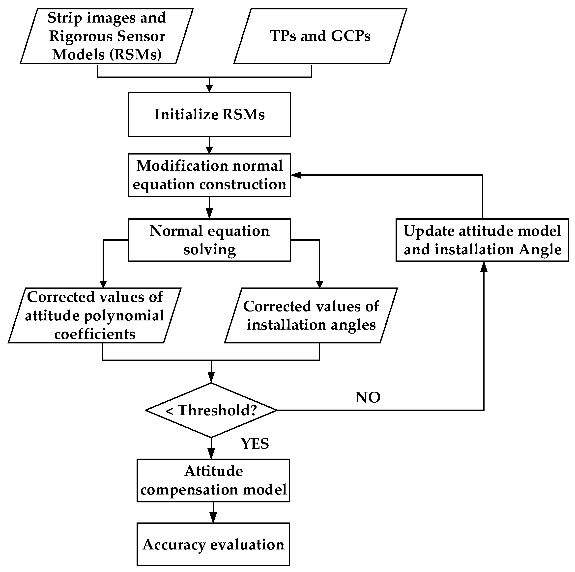
2.3. Self-Calibration Strip Adjustment Taking into Account the Installation

In the self-calibration strip adjustment scheme that considers the installation information, as shown in Figure 1, the geometric imaging models of all images are first initialized according to Equations (1), (3), and (4). Then, error equations are constructed to solve for the attitude compensation parameters and correction values of the installation angles between the multi-line array cameras.

For a multi-line array camera with $n$ loads, the unknown parameters to be solved are the $3(k+1)$ attitude polynomial coefficients (where k is the order of the polynomial) and $3(n-1)$ installation angles of other loads relative to the reference load. Therefore, for the three-line array camera of ZY-3, taking the second-order model as an example, the unknowns to be solved in the adjustment process are the nine attitude polynomial coefficients ${\phi }_i,{\omega }_i,{\kappa }_i(i=0,1,2)$, installation angle ${\phi }_{FN},{\omega }_{FN},{\kappa }_{FN}$ of the FWD camera relative to the NAD camera, and installation angle ${\phi }_{BN},{\omega }_{BN},{\kappa }_{BN}$ of the BWD camera relative to the NAD camera. For the GCPs, the unknowns are the 15 adjustment parameters mentioned above; for the TPs, the unknowns also include the corresponding object co-ordinates $(X,Y,Z)$. After initializing the rigorous geometric imaging models for all loads, an error equation was established and solved for the unknown parameters above.

For the NAD camera, the deformation of the RSM can be obtained as follows:

$$\left[\begin{array}{c}X-X_S\\ Y-Y_S\\ Z-Z_S\end{array}\right]=m\cdot {\mathit{R}}_{orbit}^{ECEF}\left(t_r\right)\cdot {\mathit{R}}_{nav}^{orbit}\left(t_r\right)\left[\begin{array}{c}tan({\psi }_y(c))\\ -tan({\psi }_x(c))\\ 1\end{array}\right]$$

(13)

The bundle adjustment accuracy is evaluated based on the number of pixels. The LOS of each pixel was used as the IOP because it can be determined by geometric calibration. Therefore, $(p_x,p_y)$ is introduced in the adjustment using the following definitions:

$$\left[\begin{array}{c}{p}_x\cdot \mu \\ p_y\cdot \mu \\ f\end{array}\right]=\left[\begin{array}{c}tan{\psi }_y\\ -tan{\psi }_x\\ 1\end{array}\right], \mathit{M}={\mathit{R}}_{orbit}^{nav}(t_r)\cdot {\mathit{R}}_{ECEF}^{orbit}\left(t_r\right)=\left[\begin{array}{ccc}{m}_{11}& m_{12}& m_{13}\\ m_{21}& m_{22}& m_{23}\\ m_{31}& m_{32}& m_{33}\end{array}\right]$$

(14)

This can be converted into a form similar to the collinear conditional equation commonly used in photogrammetric geometry processing, as follows:

$$\left\{\begin{array}{c}{p}_x=\frac{f}{\mu }\cdot \frac{m_{11}(X-X_S)+m_{12}(Y-Y_S)+m_{13}(Z-Z_S)}{m_{31}(X-X_S)+m_{32}(Y-Y_S)+m_{33}(Z-Z_S)}\\ p_y=\frac{f}{\mu }\cdot \frac{m_{21}(X-X_S)+m_{22}(Y-Y_S)+m_{23}(Z-Z_S)}{m_{31}(X-X_S)+m_{32}(Y-Y_S)+m_{33}(Z-Z_S)}\end{array}\right.$$

(15)

The processing of the FWD and BWD cameras is similar to that of the NAD camera, except that the parameter values of the matrix $\mathit{M}$ are different:

$$\begin{array}{l}{\mathit{M}}_{FN}=({\mathit{R}}_{FN}{)}^{-1}\cdot {\mathit{R}}_{orbit}^{nav}(t_r)\cdot {\mathit{R}}_{ECEF}^{orbit}(t_r)\\ {\mathit{M}}_{BN}=({\mathit{R}}_{BN}{)}^{-1}\cdot {\mathit{R}}_{orbit}^{nav}(t_r)\cdot {\mathit{R}}_{ECEF}^{orbit}(t_r)\end{array}$$

(16)

where ${\mathit{M}}_{FN}$ and ${\mathit{M}}_{BN}$ are the $\mathit{M}$ matrices corresponding to the FWD and BWD cameras, respectively.

Because the error equation is nonlinear, it is necessary to linearize Equation (15) before the least-squares adjustment. By expanding this to the first term according to the Taylor series, a linearized error equation can be obtained as follows:

$$\left\{\begin{array}{c}\begin{array}{ll}{v}_{p_x}=& \frac{\partial p_x}{\partial {\phi }_i}d{\phi }_i+\frac{\partial p_x}{\partial {\omega }_i}d{\omega }_i+\frac{\partial p_x}{\partial {\kappa }_i}d{\kappa }_i+\frac{\partial p_x}{\partial {\phi }_{FN}}d{\phi }_{FN}+\frac{\partial p_x}{\partial {\omega }_{FN}}d{\omega }_{FN}+\frac{\partial p_x}{\partial {\kappa }_{FN}}d{\kappa }_{FN}\\ & +\frac{\partial p_y}{\partial {\phi }_{BN}}d{\phi }_{BN}+\frac{\partial p_y}{\partial {\omega }_{BN}}d{\omega }_{BN}+\frac{\partial p_y}{\partial \delta {\kappa }_{BN}}d{\kappa }_{BN}+\frac{\partial p_x}{\partial X}dX+\frac{\partial p_x}{\partial Y}dY+\frac{\partial p_x}{\partial Z}dZ\\ & -(p_x-(p_x))\end{array}\\ \begin{array}{ll}{v}_{p_y}=& \frac{\partial p_y}{\partial {\phi }_i}d{\phi }_i+\frac{\partial p_y}{\partial {\omega }_i}d{\omega }_i+\frac{\partial p_y}{\partial {\kappa }_i}d{\kappa }_i+\frac{\partial p_x}{\partial {\phi }_{FN}}d{\phi }_{FN}+\frac{\partial p_x}{\partial {\omega }_{FN}}d{\omega }_{FN}+\frac{\partial p_x}{\partial {\kappa }_{FN}}d{\kappa }_{FN}\\ & +\frac{\partial p_y}{\partial {\phi }_{BN}}d{\phi }_{BN}+\frac{\partial p_y}{\partial {\omega }_{BN}}d{\omega }_{BN}+\frac{\partial p_y}{\partial \delta {\kappa }_{BN}}d{\kappa }_{BN}+\frac{\partial p_y}{\partial X}dX+\frac{\partial p_y}{\partial Y}dY+\frac{\partial p_y}{\partial Z}dZ\\ & -(p_y-(p_y))\end{array}\end{array}\right.(i=0,1,2)$$

(17)

where $\partial p/\partial {\phi }_i$, $\partial p/\partial {\omega }_i$, $\partial p/\partial {\kappa }_i$, $\partial p/\partial {\phi }_{FN}$, $\partial p/\partial {\omega }_{FN}$, $\partial p/\partial {\kappa }_{FN}$, $\partial p/\partial {\phi }_{BN}$, $\partial p/\partial {\omega }_{BN}$, $\partial p/\partial {\kappa }_{BN}$, $\partial p/\partial X$, $\partial p/\partial Y$, and $\partial p/\partial Z$ are the partial derivatives of the adjustment model with respect to each unknown parameter, respectively; $(p_x,p_y)$ are the observed values of the image point co-ordinates; $((p_x),(p_y))$ are the image point co-ordinates obtained by substituting the approximate value of the unknown into Equation(13); and $(v_{p_x},v_{p_y})$ are the corrections of the observation equation established based on the TPs or GCPs.

The indirect adjustment model can be obtained by writing Equation (17) in matrix form:

$$\mathit{V}=\left[\begin{array}{cc}\mathit{A}& \mathit{B}\end{array}\right]\left[\begin{array}{c}\mathit{t}\\ \mathit{X}\end{array}\right]-\mathit{L},\mathit{P}$$

(18)

where $\mathit{t}$ is the correction value of the attitude compensation parameter and installation angle; $\mathit{X}$ is the correction value of the ground co-ordinates of the TPs; $\mathit{L}$ is the difference between the observed and estimated values; $\mathit{A}$ is the coefficient matrix of the unknowns $\mathit{t}$; $\mathit{B}$ is the coefficient matrix of the unknowns $\mathit{X}$; and $\mathit{P}$ is the weight matrix.

$$\mathit{t}={[\begin{array}{llllllllllll}d{X}_i\hfill & d{Y}_i\hfill & d{Z}_i\hfill & d{\phi }_i\hfill & d{\omega }_i\hfill & d{\kappa }_i\hfill & d{\phi }_{FN}\hfill & d{\omega }_{FN}\hfill & d{\kappa }_{FN}\hfill & d{\phi }_{BN}\hfill & d{\omega }_{BN}\hfill & d{\kappa }_{BN}\hfill \end{array}]}^{\mathrm{T}} (i=0,1,2)$$

(19)

$$\mathit{X}={[dX,dY,dZ]}^T$$

(20)

$$\mathit{L}={[\begin{array}{cc}{p}_x-(p_x)& p_y-(p_y)\end{array}]}^T$$

(21)

For each image point, an error equation can be established in the form of Equation (17), and the corresponding normal equation is:

$$\left[\begin{array}{cc}{\mathit{A}}^{\mathit{T}}\mathit{P}\mathit{A}& {\mathit{A}}^{\mathit{T}}\mathit{P}\mathit{B}\\ {\mathit{B}}^{\mathit{T}}\mathit{P}\mathit{A}& {\mathit{B}}^{\mathit{T}}\mathit{P}\mathit{B}\end{array}\right]\left[\begin{array}{c}\mathit{t}\\ \mathit{X}\end{array}\right]=\left[\begin{array}{c}{\mathit{A}}^{\mathit{T}}\mathit{P}\mathit{L}\\ {\mathit{B}}^{\mathit{T}}\mathit{P}\mathit{L}\end{array}\right]$$

(22)

One type is typically eliminated for error equations containing two types of unknown variables. In general, the number of unknowns in $\mathit{X}$ is much larger than that in $\mathit{t}$. Therefore, it is possible to eliminate the second type of unknowns $\mathit{X}$ in Equation (21) to construct a modification equation and obtain the solution for the unknown $\mathit{t}$:

$$\mathit{t}={\left({\mathit{A}}^{\mathit{T}}\mathit{P}\mathit{A}-{\mathit{A}}^{\mathit{T}}\mathit{P}\mathit{B}\cdot {({\mathit{B}}^{\mathit{T}}\mathit{P}\mathit{B})}^{-1}\cdot {\mathit{B}}^{\mathit{T}}\mathit{P}\mathit{A}\right)}^{-1}\cdot \left({\mathit{A}}^{\mathit{T}}\mathit{P}\mathit{L}-{\mathit{A}}^{\mathit{T}}\mathit{P}\mathit{B}\cdot {({\mathit{B}}^{\mathit{T}}\mathit{P}\mathit{B})}^{-1}\cdot {\mathit{B}}^{\mathit{T}}\mathit{P}\mathit{L}\right)$$

(23)

As shown in Figure 1, the correction values of the attitude error compensation model coefficients and installation angles of the FWD and BWD cameras relative to the NAD camera were solved by using Equation (23). Then, we used the space intersection to calculate the ground co-ordinates of the tie-points and update the attitude model and installation angle when the correction values were smaller than the threshold value. The final attitude error compensation model was obtained through iterative solving, and the compensated attitude information was obtained by substituting it into the original attitude measurements.

To verify the accuracy of adjustment, it is usually necessary to calculate the root mean square error (RMSE) of the TPs or check points (CKPs). RMSE is used to reflect the deviation between the estimated value and the true value. The RMSE of TPs in the image space is calculated as follows:

$$\left\{\begin{array}{c}RMS{E}_x=\sqrt{\frac{1}{n}{\displaystyle \sum _{i=1}^n{(x_i-x_i^{\prime })}^2}}\\ RMS{E}_y=\sqrt{\frac{1}{n}{\displaystyle \sum _{i=1}^n{(y_i-y_i^{\prime })}^2}}\\ RMS{E}_{plane}=\sqrt{\frac{1}{n}{\displaystyle \sum _{i=1}^n{(x_i-x_i^{\prime })}^2+{(y_i-y_i^{\prime })}^2}}\end{array}\right.$$

(24)

where $RMS{E}_x$ is the RMSE in the scanning direction of the image; $RMS{E}_y$ is the RMSE in the flight direction of the image; $RMS{E}_{plane}$ is the RMSE in the image plane; $(x,y)$ is the true image point co-ordinates; and $(x\prime ,y\prime )$ is the estimated value of the image point co-ordinates obtained from the ground point co-ordinates after the intersection using the RSM.

The RMSE of CKPs in the object space is calculated as follows:

$$\left\{\begin{array}{c}RMS{E}_X=\sqrt{\frac{1}{N}{\displaystyle \sum _{i=1}^N{(X_i-X_i^{\prime })}^2}}\\ RMS{E}_Y=\sqrt{\frac{1}{N}{\displaystyle \sum _{i=1}^N{(Y_i-Y_i^{\prime })}^2}}\\ RMS{E}_Z=\sqrt{\frac{1}{N}{\displaystyle \sum _{i=1}^N{(Z_i-Z_i^{\prime })}^2}}\end{array}\right.$$

(25)

where $(X,Y,Z)$ is the true ground co-ordinates of the CKPs; and $(X\prime ,Y\prime ,Z\prime )$ is the estimated ground co-ordinates of the image point co-ordinates computed by the RSM.

3. Experimental Results

3.1. Experimental Datasets

The high-resolution satellite images used in this study were ZY-3 satellite Orbit 381 strip images. These images were captured on 3 February 2012, across the Taihang Mountain region. The strip covers 12 standard scenes, including FWD, BWD, and NAD images, and simultaneously provides standard scenes and strip image products. The image information is presented in

Table 1. ZY-3 satellite Orbit 381 images’ information.

Number of Scenes	Image Acquisition Time	Image Coverage Ground Size	Image Coverage (Latitude and Longitude)
12 × 3	3 February 2012	560 km × 51 km	E114.947709° N42.064374°
			E115.547510° N41.956830°
			E114.107452° N37.138009°
			E113.544067° N37.226530°

. To verify and analyze the accuracy of self-calibration bundle adjustment, 225 GCPs were used as control or check points in the experiment. GCPs are mainly measured using a static global positioning system, most of which are selected at road intersections, and the accuracy can reach 0.1 m.

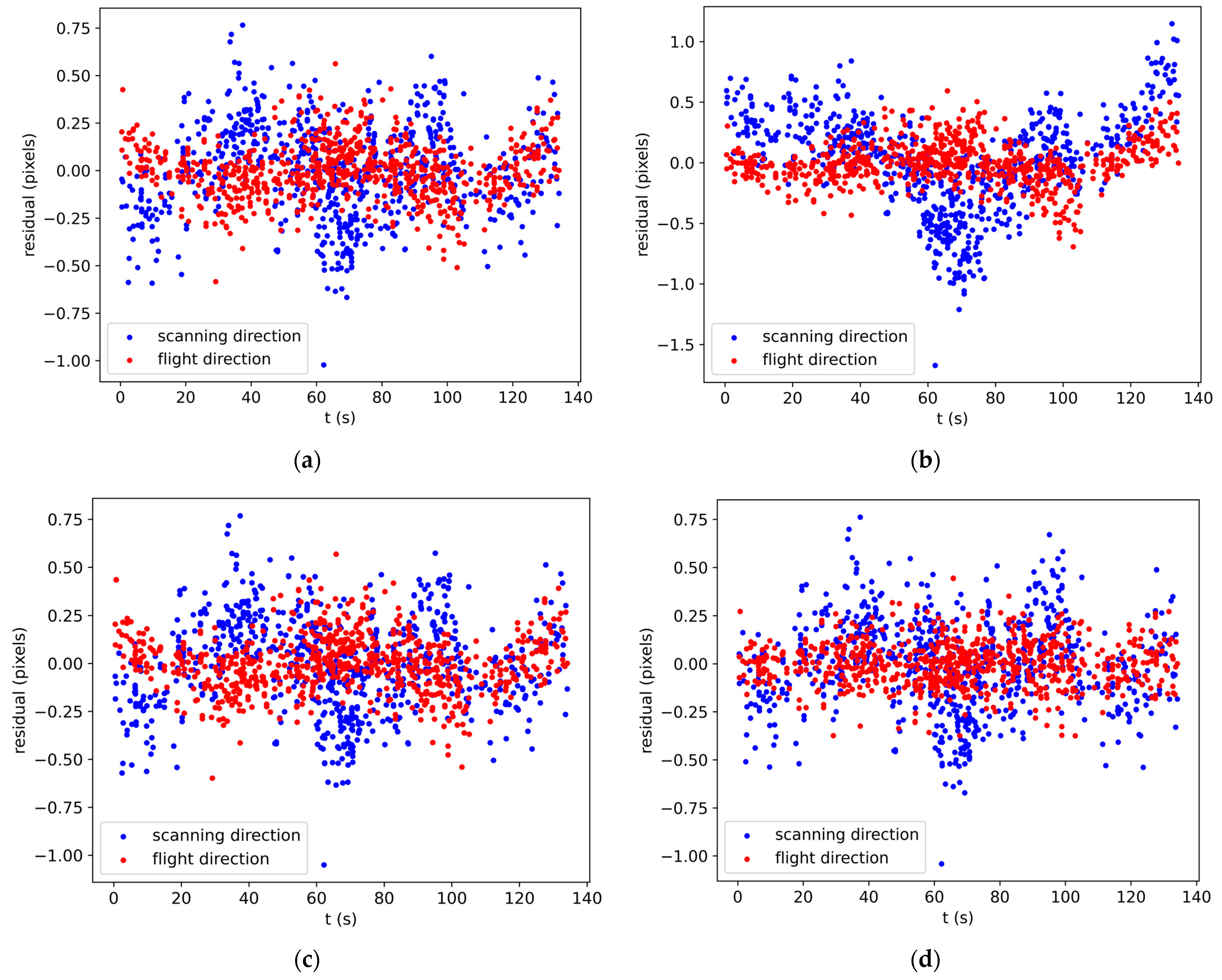
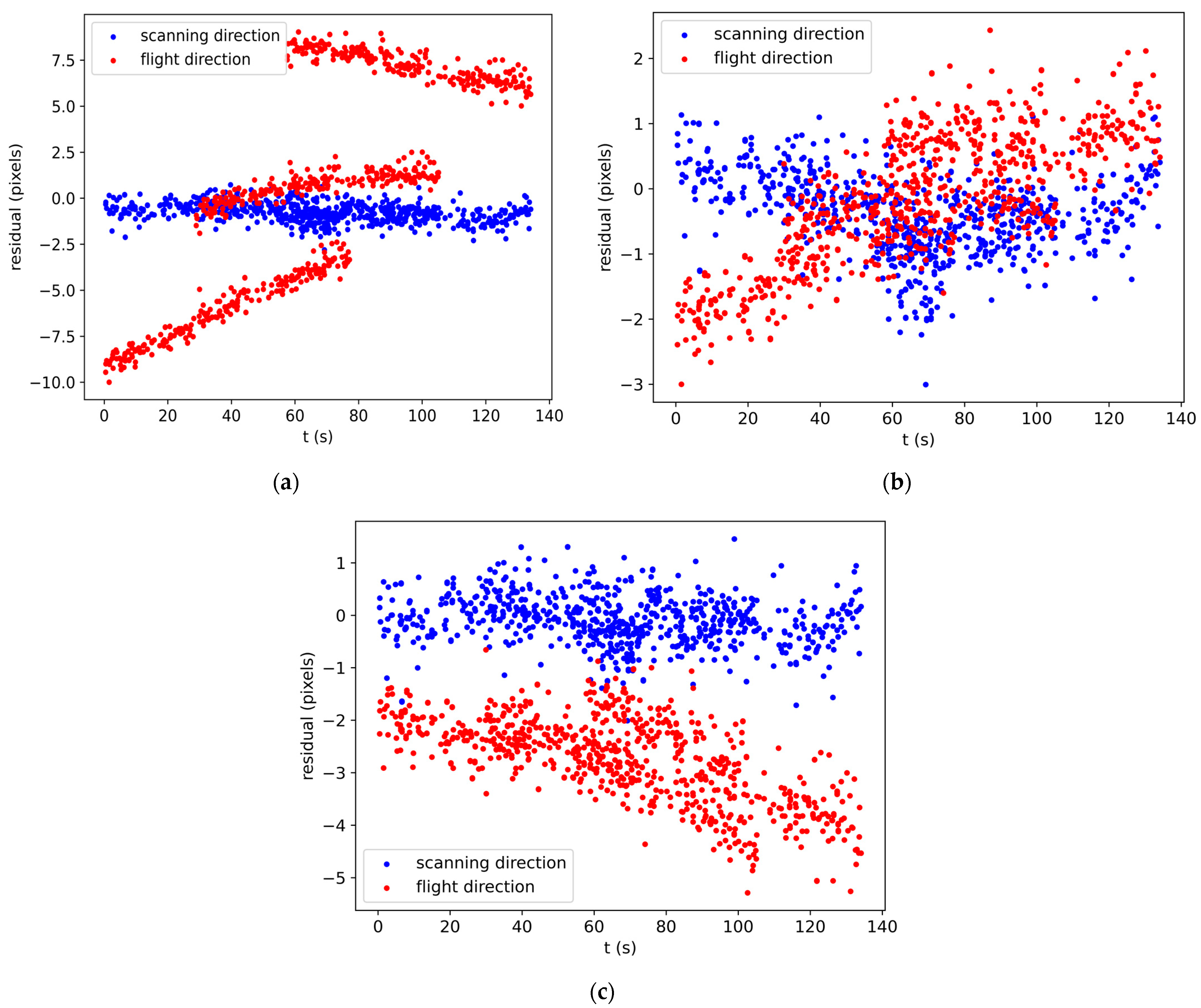
3.2. Bundle Adjustment without GCPs

Considering the installation information, we conducted adjustment experiments on an Orbit 381 image with and without a few ground control points to verify the effectiveness of the self-calibration adjustment method developed in this paper. This section presents the results of the adjustment experiments without ground control points.

The bundle block adjustment of high-resolution satellite images without ground control points is also referred to as free-net adjustment. The free-net adjustment of stereo images mainly utilizes the epipolar and tie-point constraints, which leads to consistent attitude uncertainty. Based on the consistent attitude error of the same satellite platform, we established an integrated adjustment scheme that considers the installation information.

In this study, four experimental plans were designed to synthesize and evaluate the experimental results. The details are as follows:

Plan A:

Three-line-array-cameras independent adjustment with first-order attitude compensation model.

Plan B:

Self-calibration adjustment with translation attitude compensation model considering installation.

Plan C:

Self-calibration adjustment with first-order attitude compensation model considering installation.

Plan D:

Self-calibration adjustment with second-order attitude compensation model considering installation.

Among them, Plan A is the most commonly used method in the current study of multi-line array satellite image adjustment, and the independent adjustment of the three-line array cameras is to establish different attitude compensation models for the FWD, BWD, and NAD cameras, and the adjustment unit is a single load. Plans B, C, and D are developed in this paper to establish a unified attitude compensation model for the three cameras by introducing the installation angle between the three-line array cameras. The only difference among these three schemes is the polynomial order used in the attitude compensation model. In this section, the four aforementioned plans are implemented without GCPs.

The accuracy indices of the satellite images include the accuracy in the image space and object space. Bundle adjustment was performed on the Orbit 381 image under the four schemes above, and all GCPs were used as CKPs. After the adjustment, the root mean square errors (RMSEs) of the TPs in the image space are listed in

Table 2. The RMSE of TPs in the image space after adjustment without GCPs for Orbit 381.

Plan	The RMSE of TPs in the Image Space (Pixels)
	Scanning Direction	Flight Direction	Plane
Plan A	0.240	0.145	0.280
Plan B	0.402	0.172	0.438
Plan C	0.241	0.145	0.281
Plan D	0.238	0.117	0.265

, and those of the CKPs in the object space are listed in

Table 3. The RMSE of CKPs in the object space after adjustment without GCPs for Orbit 381.

Plan	The RMSE of CKPs in the Object Space (m)
	East	North	Plane	Height
Plan A	3.873	2.553	4.639	53.270
Plan B	7.293	15.638	17.255	53.918
Plan C	2.308	3.217	3.960	53.287
Plan D	6.110	4.518	7.599	53.892

. The trend of the residuals of the TPs with the imaging time was plotted as shown in Figure 2, where the imaging time of the connection point can be interpolated from the imaging time of each row of the image. The blue points are the residuals of the TPs in the scanning direction, and the red points are the residuals in the flight direction.

Table 2 and Table 3 show that the self-calibration adjustment scheme based on the translation attitude compensation model (Plan B) has a slightly worse accuracy in the image and object spaces than the three-line array independent adjustment scheme (Plan A). This is because the main errors of the ZY-3 three-line array camera are the attitude drifts in the pitch and roll angles at different drift rates [30], which means that utilizing only the translation parameter is insufficient to compensate for the error terms in the attitude. Therefore, we further introduced drift parameters based on the first-order attitude compensation model to carry out a self-calibration adjustment (Plan C) for Orbit 381, and the accuracy after adjustment reached the same level as that of Plan A.

To verify whether the scheme developed in this study correctly calculated the installation relationship between the three-line array cameras, we calculated the reprojection errors of the CKPs under the above three schemes based on the real ground co-ordinates of the CKPs. We plotted their distributions, as shown in Figure 3. It can be seen that the distribution of the reprojection errors of the CKPs in the flight direction is presented in the form of three parallel lines when Plan A is used for the adjustment of the three-line array images. Figure 3b,c show that the distribution of the reprojection errors of the CKPs in the flight direction is already continuous when Plans B and C are used for the adjustment of the three-line array images. This shows that, in the absence of ground control points, the self-calibration adjustment scheme based on a translation model or a first-order model that considers the installation can compute the installation relationship between the three-line array cameras.

However, as shown in Figure 2, the distributions of the residuals of the TPs with imaging time after an adjustment based on Plans A, B, and C are chaotic, and the consistency of the geometric accuracy is poor. Therefore, we utilized the second-order attitude compensation model for the self-calibration adjustment (Plan D). The consistency of the residuals in the flight direction of the TPs was significantly improved after the adjustment, and the obvious error jitter was eliminated; however, the object space plane accuracy decreased slightly. This is because the number of unknown parameters to be solved increased, and it is difficult to solve them using only the internal constraints of images without ground control information.

3.3. Bundle Adjustment with GCPs

In Section 3.2, the experimental results of the adjustment without GCP show that the image-space and object-space accuracy of the image do not improve after using Plan B for adjustment. Therefore, the adjustment experiments with GCPs in this section focus only on Plans A, C, and D for a comparative analysis.

Three different GCP layout schemes were set up for the cases of 4, 16, and 27 GCPs when performing adjustments with GCPs. When four GCPs were used, the GCPs were distributed at the four corner points of the entire track image. When 16 and 27 GCPs were used, the GCPs were evenly distributed in the image. To verify the adjustment accuracy under different GCP distributions, we considered all the remaining unused control points as CKPs and calculated the object-space RMSE of the CKPs as a reflection of the object space accuracy after adjustment. The RMSEs of the TPs in the image space after adjustment are listed in

Table 4. The RMSE of TPs in the image space after adjustment with GCPs for Orbit 381.

GCP Layout Scheme	Plan	The RMSE of TPs in the Image Space (Pixels)
		Scanning Direction	Flight Direction	Plane
4 GCPs	Plan A	0.248	0.145	0.287
	Plan C	0.249	0.167	0.300
	Plan D	0.246	0.152	0.289
16 GCPs	Plan A	0.269	0.175	0.321
	Plan C	0.269	0.194	0.331
	Plan D	0.263	0.181	0.319
27 GCPs	Plan A	0.290	0.218	0.363
	Plan C	0.290	0.248	0.382
	Plan D	0.288	0.229	0.368

, and those of the CKPs in the object space are listed in

Table 5. The RMSE of CKPs in the object space after adjustment with GCPs for Orbit 381.

GCP Layout Scheme	Plan	The RMSE of CKPs in the Object Space (m)
		East	North	Plane	Height
4 GCPs	Plan A	1.680	1.385	2.177	1.571
	Plan C	1.679	1.355	2.158	2.313
	Plan D	1.297	1.332	1.859	1.876
16 GCPs	Plan A	1.333	1.331	1.884	1.505
	Plan C	1.328	1.340	1.887	2.275
	Plan D	1.309	1.285	1.834	1.717
27 GCPs	Plan A	1.259	1.341	1.839	1.340
	Plan C	1.260	1.343	1.841	2.224
	Plan D	1.233	1.298	1.790	1.360

.

Table 4 and Table 5 show that Plan C can achieve planimetric accuracy comparable to Plan A under all three GCP layout schemes, but the elevation accuracy will be slightly worse. This is because the attitude error of ZY-3 is locally linear. Therefore, the accuracy of the attitude compensation by building a segment of the linear model for each camera individually is better than the accuracy of the attitude compensation by using a uniform linear model for all cameras. When we further used the second-order attitude compensation model for adjustment (Plan D), the plane accuracies of the images can reach a comparable level with Plan A under all three GCP layout schemes; the elevation accuracies will be slightly worse when there are only sparse GCPs, and the elevation accuracies of those two schemes are comparable when the number of GCPs reaches 27. In summary, by comparing the RMSE, it can be seen that, with the increase in the number of GCPs, the accuracies of the self-calibration adjustment scheme considering the installation developed in this paper are all improved.

To further verify whether the effects of different adjustment plans were similar or statistically significantly different, we performed statistical significance tests on the errors after adjustment using Student’s t-test at a significance level of α = 0.05. We conducted four sets of tests. The first two groups of tests were comparisons between different schemes with identical GCP layout schemes (4GCP), and the results are shown in

Table 6. Results of t-tests between different adjustment plans (with 4 GCPs).

Test Scheme	Comparison Plan	Plane		Height
		ME (m)	p-Value	ME (m)	p-Value
Test 1	Plan A	1.904	0.924	0.751	0.455
	Plan C	1.914		0.618
Test 2	Plan C	1.914	2.190 × 10−4	0.618	0.194
	Plan D	1.551		0.864

. Table 6 shows that the plane and elevation accuracies of Plan C are not significantly different from those of Plan A. However, there is a significant difference in the plane accuracy of Plan D compared to Plan C, with an improvement in plane accuracy indicated by the mean error (ME). It indicates that the self-calibration adjustment scheme based on the first-order model can achieve a comparable accuracy with the traditional scheme, while using the second-order model further enhances the plane accuracy of images. Therefore, using the second-order attitude compensation model in the developed adjustment scheme proves to be more effective.

Based on the analysis above, we compared the effects under different GCP layout schemes for Plan D. The results are shown in

Table 7. Results of t-tests between the different GCP layout schemes for Plan D.

Test Scheme	GCP Layout Scheme	Plane		Height
		ME (m)	p-Value	ME (m)	p-Value
Test 3	4 GCPs	1.551	0.895	0.864	0.009
	16 GCPs	1.538		0.436
Test 4	16 GCPs	1.538	0.676	0.436	0.020
	27 GCPs	1.496		0.079

. Table 7 shows that, with the increase in the number of GCPs, there is no significant difference between the plane accuracies after adjustment, and the MEs are relatively close to each other, which indicates that using only four GCPs can be sufficient to satisfy our needs. The elevation accuracy improved with the increase in the number of GCPs, but the MEs and RMSEs (Table 5) of elevation show that the improvement in elevation accuracy is limited. Moreover, as the number of GCPs increases, the measurement cost of GCPs also increases. Therefore, when there are not enough available GCPs due to the conditions, four GCPs can satisfy the application requirements.

Table 5 shows that, when using only four GCPs with the developed Plan D for bundle adjustment, the image plane and elevation accuracies are 1.859 m and 1.876 m. The plane accuracy is comparable to that based on 16 GCPs or more GCPs using the traditional scheme. Combined with the results of the Student’s t-test, this further demonstrates that, compared to the traditional scheme, the self-calibration adjustment scheme based on the second-order attitude compensation model that considers the installation developed in this paper not only considers the consistency of the same-platform error of the multi-line array cameras but also ensures image accuracy with the introduction of only sparse GCPs.

4. Discussion

The variation in the space thermal environment in orbit causes the attitude of the high-resolution multi-line array satellite to vary over time and space, resulting in a positioning error of the acquired remote sensing image showing the characteristics of temporal and spatial variation, which becomes the key factor restricting high-resolution multi-line array satellite direct positioning with a high accuracy. Bundle block adjustment is a key technology for error correction in large-scale and multi-view satellite images. Owing to the dynamic change in the installation error of a high-resolution satellite multi-line array camera, it is crucial to construct the attitude and installation of a decoupled high-resolution multi-line array satellite image block adjustment. However, existing studies usually assume that multi-line array data are independent of each other without considering the consistency of the same-platform error and the correlation of the attitude error. The method developed in this paper makes full use of the geometric constraints of multi-line arrays on the same platform to ensure the positioning accuracy of the image, while reducing the need for external control.

In the absence of ground control points, we conducted self-calibration adjustment experiments on the ZY-3 images, considering the installation based on three different orders of attitude compensation models. Compared with the traditional three-line array independent adjustment scheme, the accuracy of the adjustment scheme based on the translation model is slightly worse because there is an attitude drift in the ZY-3 image, making the translation model insufficient to compensate for it. However, at this time, it has been able to calculate the installation relationship between the three-line array cameras. The adjustment scheme based on the first-order model can achieve an accuracy comparable to that of the traditional scheme; however, the distribution of the residuals in the image space is still relatively chaotic. Therefore, we introduced an adjustment scheme based on a second-order model. The consistency of the residuals in the flight direction of the TPs was significantly improved after the adjustment, and the obvious error jitter was eliminated; however, the object space plane accuracy decreased slightly. This is because the number of unknown additional parameters to be solved increases as the order of the attitude compensation model increases, and it is difficult to solve them using only the internal constraints of the image without ground control information.

In the adjustment experiments without GCPs, we found that the adjustment scheme based on the translation attitude compensation model did not improve the accuracy of the image. Therefore, in the adjustment with GCPs, we discuss only self-calibration adjustment schemes based on the first-order and second-order attitude models. In this study, we set up three different control point placement schemes: 4GCP, 16GCP, and 27GCP. Among all three GCP layout schemes, the adjustment scheme based on the first-order model achieved a planimetric accuracy comparable to that of the traditional three-line array independent adjustment scheme; however, the elevation accuracy was slightly worse. This is because the attitude error behaves locally linearly. Therefore, a different first-order attitude compensation model for each camera will provide a better accuracy than using the same first-order model for all cameras for attitude compensation. When we adopt the second-order attitude compensation model for the adjustment, the plane accuracies of the images under all three GCP layout schemes are all comparable to those of the traditional schemes. When there are only sparse GCPs, the elevation accuracy is slightly worse, and, when the number of GCPs reaches 27, the elevation accuracies of the two schemes are comparable. To further validate the effectiveness of the developed adjustment scheme, we performed statistical significance tests on the errors after an adjustment using Student’s t-test. The results of the t-tests indicate that the developed self-calibration adjustment scheme based on the first-order model can achieve a comparable accuracy with the traditional scheme, and the plane accuracy of images is improved when using the second-order model. However, with the increase in the number of GCPs, the improvement of the adjustment accuracy is limited. When GCPs are deployed only at the four corner points of the image, the image plane accuracy and elevation accuracy after a self-calibration adjustment are 1.859 m and 1.876 m, respectively, which can reach a similar plane accuracy after the traditional adjustment scheme with 16 or more GCPs. It indicates that the sparse GCP can also basically meet our application requirements. In summary, the method developed in this paper can reduce the need for external control as much as possible while ensuring image positioning accuracy.

5. Conclusions

This paper develops a self-calibration adjustment scheme for high-resolution stereo satellite images that utilizes the geometrical constraints of satellite multi-loads on the same platform, introduces the installation relationship between multiple loads, and utilizes a unified model to compensate for the attitude errors of satellite images. This method provides a new idea for the attitude compensation of high-resolution multi-line array satellite images. Using this method on ZY-3 satellite images, when only GCPs are at the four corner points of the image, the image plane and elevation accuracies were 1.86 m and 1.87 m, respectively. Combined with the results of the significance tests, this demonstrates that the method developed in this paper can achieve a comparable accuracy to the traditional adjustment using more GCPs. It indicates that the method can reduce the need for external control as much as possible while ensuring image positioning accuracy.

References

1. Li, D.; Wang, M. A review of high resolution optical satellite surveying and mapping technology. Spacecr. Recovery Remote Sens. 2020, 41, 1–11. [Google Scholar]
2. Tadono, T.; Shimada, M.; Watanabe, M.; Hashimoto, T.; Iwata, T. Calibration and validation of PRISM onboard ALOS. Int. Arch. Photogramm. Remote Sens. Spat. Inf. Sci. 2004, 35, 13–18. [Google Scholar]
3. Bouillon, A.; Bernard, M.; Gigord, P.; Orsoni, A.; Rudowski, V.; Baudoin, A. SPOT 5 HRS geometric performances: Using block adjustment as a key issue to improve quality of DEM generation. ISPRS J. Photogramm. Remote Sens. 2006, 60, 134–146. [Google Scholar] [CrossRef]
4. Muralikrishnan, S.; Pillai, A.; Narender, B.; Reddy, S.; Venkataraman, V.R.; Dadhwal, V. Validation of Indian national DEM from Cartosat-1 data. J. Indian Soc. Remote Sens. 2013, 41, 1–13. [Google Scholar] [CrossRef]
5. Wang, R.; Hu, X.; Wang, J. Photogrammetry of mapping satellite-1 without ground control points. Acta Geod. Cartogr. Sin. 2013, 42, 1–5. [Google Scholar]
6. Cao, H.; Zhang, X.; Zhao, C.; Xu, C.; Mo, F.; Dai, J. System design and key technolongies of the GF-7 satellite. Chin. Space Sci. Technol. 2020, 40, 1. [Google Scholar]
7. Barazzetti, L.; Roncoroni, F.; Brumana, R.; Previtali, M. Georeferencing accuracy analysis of a single worldview-3 image collected over milan. Int. Arch. Photogramm. Remote Sens. Spat. Inf. Sci. 2016, XLI-B1, 429–434. [Google Scholar] [CrossRef]
8. Greslou, D.; de Lussy, F.; Amberg, V.; Dechoz, C.; Lenoir, F.; Delvit, J.-M.; Lebègue, L. Pleiades-HR 1A&1B image quality commissioning: Innovative geometric calibration methods and results. In Proceedings of the Earth Observing Systems XVIII; SPIE: San Diego, CA, USA, 2013; p. 886611. [Google Scholar]
9. Luthcke, S.; Zelensky, N.; Rowlands, D.; Lemoine, F.; Williams, T. The 1-centimeter orbit: Jason-1 precision orbit determination using GPS, SLR, DORIS, and altimeter data special issue: Jason-1 calibration/validation. Mar. Geod. 2003, 26, 399–421. [Google Scholar] [CrossRef]
10. Zhao, C.; Tang, X. Precise orbit determination for the ZY-3 satellite mission using GPS receiver. J. Astronaut. 2013, 34, 1202–1206. [Google Scholar]
11. Jiang, Y.; Zhang, G.; Tang, X.; Zhu, X.; Qin, Q.; Li, D.; Fu, X. High accuracy geometric calibration of ZY-3 three-line image. Acta Geod. Cartogr. Sin. 2013, 42, 523–529. [Google Scholar]
12. Hofmann, O.; Navé, P.; Ebner, H. DPS-A Digital Photogrammetric System for producing digital elevation models and orthophotos by means of linear array scanner imagery. Photogramm. Eng. Remote Sens. 1984, 50, 1135–1142. [Google Scholar]
13. Wang, R. Satellite Photogrammetric Principle for Three-Line-Array CCD Imagery; Surveying and Mapping Press: Beijing, China, 2016; pp. 53–54. [Google Scholar]
14. Wang, R.; Hu, X.; Wang, X.; Yang, J. The construction and application of mapping satellite-1 engineering. J. Remote Sens. 2012, 16, 2–5. [Google Scholar]
15. Ebner, H.; Kornus, W.; Ohlhof, T.; Putz, E. Orientation of MOMS-02/D2 and MOMS-2P/PRIRODA imagery. ISPRS J. Photogramm. Remote Sens. 1999, 54, 332–341. [Google Scholar] [CrossRef]
16. Poli, D. A rigorous model for spaceborne linear array sensors. Photogramm. Eng. Remote Sens. 2007, 73, 187–196. [Google Scholar] [CrossRef]
17. Weser, T.; Rottensteiner, F.; Willneff, J.; Poon, J.; Fraser, C.S. Development and testing of a generic sensor model for pushbroom satellite imagery. Photogramm. Rec. 2008, 23, 255–274. [Google Scholar] [CrossRef]
18. Kim, T.; Dowman, I. Comparison of two physical sensor models for satellite images: Position–rotation model and orbit–attitude model. Photogramm. Rec. 2006, 21, 110–123. [Google Scholar] [CrossRef]
19. Li, R.; Hwangbo, J.; Chen, Y.; Di, K. Rigorous photogrammetric processing of HiRISE stereo imagery for Mars topographic mapping. IEEE Trans. Geosci. Remote Sens. 2011, 49, 2558–2572. [Google Scholar]
20. Radhadevi, P.; Nagasubramanian, V.; Mahapatra, A.; Solanki, S.; Sumanth, K.; Varadan, G. Potential of high-resolution Indian remote sensing satellite imagery for large scale mapping. In Proceedings of the ISPRS Hannover Workshop, High-Resolution Earth Imaging for Geospatial Information, Hannover, Germany, 2–5 June 2009. [Google Scholar]
21. Rottensteiner, F.; Weser, T.; Lewis, A.; Fraser, C.S. A strip adjustment approach for precise georeferencing of ALOS optical imagery. IEEE Trans. Geosci. Remote Sens. 2009, 47, 4083–4091. [Google Scholar] [CrossRef]
22. Di, K.; Liu, Y.; Liu, B.; Peng, M.; Hu, W. A Self-Calibration Bundle Adjustment Method for Photogrammetric Processing of Chang’E-2 Stereo Lunar Imagery. IEEE Trans. Geosci. Remote Sens. 2013, 52, 5432–5442. [Google Scholar]
23. Zhang, Y.; Zheng, M.; Wang, X.; Huang, X. Strip-based bundle adjustment of Mapping Satellite-1 three-line array imagery. J. Remote Sens. Beijing 2012, 16, 84–89. [Google Scholar]
24. Zheng, M.; Zhang, Y.; Zhu, J.; Xiong, X. Self-calibration adjustment of CBERS-02B long-strip imagery. IEEE Trans. Geosci. Remote Sens. 2015, 53, 3847–3854. [Google Scholar] [CrossRef]
25. Cao, J.; Yuan, X.; Fu, J.; Gong, J. Precise sensor orientation of high-resolution satellite imagery with the strip constraint. IEEE Trans. Geosci. Remote Sens. 2017, 55, 5313–5323. [Google Scholar] [CrossRef]
26. Li, D. China’s first civilian three-line-array stereo mapping satellite: ZY-3. Acta Geod. Cartogr. Sin. 2012, 41, 317–322. [Google Scholar]
27. Grodecki, J.; Dial, G. Block adjustment of high-resolution satellite images described by rational polynomials. Photogramm. Eng. Remote Sens. 2003, 69, 59–68. [Google Scholar] [CrossRef]
28. Zhang, Y.; Zheng, M.; Xiong, J.; Lu, Y.; Xiong, X. On-orbit geometric calibration of ZY-3 three-line array imagery with multistrip data sets. IEEE Trans. Geosci. Remote Sens. 2013, 52, 224–234. [Google Scholar] [CrossRef]
29. Zhang, Y.; Zheng, M.; Xiong, X.; Xiong, J. Multistrip bundle block adjustment of ZY-3 satellite imagery by rigorous sensor model without ground control point. IEEE Geosci. Remote Sens. Lett. 2014, 12, 865–869. [Google Scholar] [CrossRef]
30. Pan, H.; Tao, C.; Zou, Z. Precise georeferencing using the rigorous sensor model and rational function model for ZiYuan-3 strip scenes with minimum control. ISPRS J. Photogramm. Remote Sens. 2016, 119, 259–266. [Google Scholar] [CrossRef]
31. Yuan, X.; Yu, X. Calibration of angular systematic errors for high resolution satellite imagery. Acta Geod. Cartogr. Sin. 2012, 41, 385–392. [Google Scholar]
32. Cao, J.; Fu, J.; Yuan, X.; Gong, J. Nonlinear bias compensation of ZiYuan-3 satellite imagery with cubic splines. ISPRS J. Photogramm. Remote Sens. 2017, 133, 174–185. [Google Scholar] [CrossRef]
33. Tao, C.V.; Hu, Y. A comprehensive study of the rational function model for photogrammetric processing. Photogramm. Eng. Remote Sens. 2001, 67, 1347–1358. [Google Scholar]
34. Poli, D.; Toutin, T. Review of developments in geometric modelling for high resolution satellite pushbroom sensors. Photogramm. Rec. 2012, 27, 58–73. [Google Scholar] [CrossRef]
35. Liu, C.; Zhang, Y.; Fan, D.; Lei, R.; Dai, H. Self-calibration Block Adjustment for Three-line-array Image of ZY-3. Acta Geod. Cartogr. Sin. 2014, 43, 1046. [Google Scholar]
Figure 1. Flow chart of self-calibration strip adjustment, taking into account the installation.
Remotesensing 16 02196 g001
Figure 2. Residuals distribution of TPs of each plan after bundle adjustment without GCP of Orbit 381: (a) Plan A; (b) Plan B; (c) Plan C; and (d) Plan D.
Remotesensing 16 02196 g002
Figure 3. Reprojection errors of the CKPs: (a) Plan A; (b) Plan B; and (c) Plan C.
Remotesensing 16 02196 g003