Abstract
Traditional radar target detectors, which are model-driven, often suffer remarkable performance degradation in complex clutter environments due to the weakness in modeling the unpredictable clutter. Deep learning (DL) methods, which are data-driven, have been introduced into the field of radar target detection (RTD) since their intrinsic non-linear feature extraction ability can enhance the separability between targets and the clutter. However, existing DL-based detectors are unattractive since they require a large amount of independent and identically distributed (i.i.d.) training samples of target tasks and fail to be generalized to the other new tasks. Given this issue, incorporating the strategy of meta-learning, we reformulate the RTD task as a few-shot classification problem and develop the Inter-frame Contrastive Learning-Based Meta Detector (IfCMD) to generalize to the new task efficiently with only a few samples. Moreover, to further separate targets from the clutter, we equip our model with Siamese architecture and introduce the supervised contrastive loss into the proposed model to explore hard negative samples, which have the targets overwhelmed by the clutter in the Doppler domain. Experimental results on simulated data demonstrate competitive detection performance for moving targets and superior generalization ability for new tasks of the proposed method.
1. Introduction
Radar target detection (RTD) in complex clutter backgrounds has been a long-standing challenge for ground-based warning radar [1,2], as small or slow-moving targets are prone to being overwhelmed by the strong clutter. Three main ways to improve moving-target detection performance in clutter backgrounds have emerged:
- (1)
- Some researchers are devoted to improving the signal-to-clutter plus noise ratio (SCNR) of targets. One way is to suppress the clutter, and the representatives are moving target indication (MTI) [3,4,5] and adaptive filtering methods. But MTI is vulnerable to dynamic clutter [6], and adaptive filtering methods require prior knowledge of the target. Another way is to enhance the power of the target, such as the moving-target detection (MTD) [7] method. Its prevalence stems from the capability of coherently integrating the energy of the target and separating it from the clutter (due to their considerable speed difference) in the Doppler domain. However, the low-speed property of the slow-moving target causes its coupling with the clutter within the Doppler domain. As a result, the detection performance remains unsatisfactory after MTD.
- (2)
- Another group of methods detects targets by estimating the power level of the clutter background and calculating the detection threshold under the condition of the constant false alarm rate (CFAR) [8,9,10]. This type of method, called the CFAR detection method, typically assumes that the amplitude of the clutter obeys homogeneous Rayleigh distribution. So, the power level of the background can be estimated using reference cells adjacent to the cell under test (CUT) in space. Until now, many efforts and contributions have been devoted to the research and application of CFAR detection schemes. However, the non-homogeneous clutter in realistic environments hinders the effectiveness of these CFAR detectors [11,12,13].
- (3)
- The third kind of method models the clutter in space with a settled probabilistic distribution and estimates the clutter precisely [14,15]. Typically, a test statistic is deduced by assuming a known distribution form for the clutter beforehand. Then, the clutter covariance matrix (CCM), estimated based on the secondary data collected from the vicinity of the CUT, is employed in the test statistic for subsequent detection. Many relative methods have been proposed over the past years [16,17,18,19]. However, due to the sensitivity to the background clutter distribution, these methods suffer from target detection performance degradation in low-altitude backgrounds where the clutter is complex and uncontrollable.
More recently, deep learning (DL) methods [20] have been increasingly applied to solve bottleneck problems in the field of radar due to their powerful feature extraction and parallel data-processing capabilities [21,22,23]. Distinct from traditional approaches that require crafting suitable models based on physical mechanisms, DL-based RTD methods rely on plenty of available data to train a neural network for effective detection, which can be roughly divided into two groups, i.e., supervised and unsupervised. Specifically, supervised approaches cast RTD as a classification problem and train a neural network using the labeled data to distinguish the target class from the clutter class [24,25,26]. Differently, unsupervised methods draw inspiration from anomaly detection and build a network to define a region in the feature space to represent the behavior of clutter (target-absent) samples [27,28]. As a result, target-present samples can be detected as outliers. However, current approaches mainly concentrate on improving detection performance for fast targets in the clutter environment, which can be ineffective for hard-to-detect targets (such as small or slow-moving targets) since the clutter only differs slightly from the target. In addition, more generalization ability to new tasks is needed to ensure DL-based RTD methods can be applied in flexible and changing real-world environments. Therefore, developing effective RTD methods with sufficient generalization capabilities is crucial for real-world target detection.
Given the above issues, in this paper, we propose a novel DL-based RTD framework, called Inter-frame Contrastive Learning-Based Meta-Detector (IfCMD), to improve the detection performance of moving targets and ensure robustness for the unseen RTD task. The inspiration comes from the discovery that the stability of land clutter is more guaranteed over a short time than in space, as shown in Figure 1.
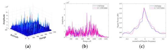
Figure 1.
Characteristics of the measured ground clutter. (a) Range–azimuth–amplitude image of measured ground clutter of a frame. This subfigure indicates that the spatial distribution of ground clutter in practice is complex and inhomogeneous. (b) Comparison of signal amplitude between neighboring frames. This subfigure is displayed to demonstrate that the amplitude of the clutter signal at the same location varies little between neighboring frames. (c) Comparison of Doppler spectrum in a range cell between neighboring frames. It can be seen that the Doppler characteristic of the clutter signal at the same location varies little between neighboring frames.
Consequently, instead of modeling the clutter spatially, we model the temporal characteristic of the clutter for more effective target detection.
In this paper, following the custom transforming moving-target detection task as the classification problem in DL, we design IfCMD in four steps. Firstly, we define the differential Doppler information (DDI) to portray the variation in the Doppler characteristic between the current coherent pulse interval (CPI) and the previous CPI. Given the distinctive nature of the Doppler characteristic and its variation between adjacent frames for RTD, we fuse the complete Doppler information (CDI) within the current CPI and the DDI together as the form of samples in each range cell. Then, to improve the detection performance of hard-to-detect targets, we adopt contrastive learning (CL) [29,30,31], an emerging strategy in machine learning, to design the network architecture and the loss function. Since the hard-to-detect target-present samples can be viewed as hard negative samples compared to target-absent samples, a supervised contrastive loss [32] is implemented to train the network, enabling hard negative samples to be better segregated in feature space. As the commonly used architecture in the CL paradigm, the Siamese network [33,34] is naturally adopted as our network architecture to aid this separation. Moreover, to equip our model with excellent generalization capability, a pioneer strategy for few-shot learning, meta-learning [35,36], is introduced to train our model. By capturing the across-task knowledge in the meta-training stage with the episodic training paradigm, the optimized model is able to efficiently generalize to the new task with only a few available samples in the meta-testing stage. Finally, label prediction is realized in the Siamese network by determining whether the test sample is of the same class as a known labeled one. Inspired by this, we introduce a fresh detection strategy to determine the presence of a target in a CUT efficiently. Specifically, in the latent space, the probability density function (PDF) of the similarity between the positive pair consisting of target-absent samples can be estimated. Leveraging this PDF and the preset probability of false alarm (Pfa), we derive a detection threshold for target detection. This threshold allows for a fair performance comparison with traditional methods under the same Pfa, demonstrating the superiority of our strategy. To our knowledge, this is the first work integrating meta-learning and CL into the context of RTD for warning radar systems. The experimental results show that the proposed method exhibits superior generalization capabilities and significantly improves the detection performance of hard-to-detect targets compared to established classical radar target detectors.
In summary, our contributions are as follows:
- Inspired by the discovery that clutter remains stable between adjacent frames, we provide a novel DL-based RTD approach in which the signal variation in the range cell between adjacent frames is utilized to determine if a target is present.
- We adopt the supervised contrastive loss and the Siamese network architecture to encourage learning from hard negative samples to promote the detection of moving targets.
- We induce the meta-learning paradigm to equip our model with superior generalization ability to the new task.
- We design a novel detection strategy that can accomplish RTD tasks efficiently and assess the detection performance statistically under the CFAR condition.
The rest of this paper is organized as follows. Section 2 introduces related work. Section 3 elaborates on the proposed detector. Section 4 showcases simulation results and analysis, and Section 5 presents the performance of IfCMD on measured data. Section 6 provides discussion about IfCMD. Section 7 presents the conclusions drawn from our findings. Notation: In this paper, denotes the transpose operation. Each signal denoted with is target-absent.
2. Related Work
2.1. Meta-Learning
Meta-learning [37,38,39], also known as “learning to learn”, is a machine learning paradigm inspired by the human ability to acquire new concepts and skills quickly and efficiently. Generally, a good meta-learning model is expected to adapt or generalize well to new tasks and environments that have never been encountered during training [40]. The adaptation process, which occurs during testing, is essentially a mini-learning session with access to only a limited number of new task examples [41]. To achieve this goal, the model is typically trained over a variety of learning tasks and optimized for the best performance on a distribution of tasks . Each task is associated with a dataset D that contains both input samples and ground truth labels. Thus, the optimal model parameters are
where is the loss function for each task, such as the cross-entropy function for a classification task.
As a representative instantiation of meta-learning in the field of supervised learning, few-shot classification [42] further splits the dataset D of each task into two parts: a support set S for learning and a query set Q for evaluation. The optimization objective can thus be understood as reducing the prediction error on data samples with unknown labels (i.e., the query set Q) given a small support set S for “fast learning”.
There are three common approaches to meta-learning: metric-based, model-based, and optimization-based. Particularly, optimization-based methods [39,43] revolve around enhancing the optimization process itself to facilitate faster adaptation to new tasks. Model-based approaches [44] aim to learn a good base model so that the prior knowledge encoded in it can accelerate the learning of novel tasks. Metric-based methods [45,46] focus on learning a similarity metric or distance function that can effectively generalize across tasks. The core idea lies in mapping input data points into a metric space where instances with similar structures or characteristics are close to each other. Since a majority of the state-of-the-art meta-learning approaches are metric-based methods, this paper also exploits a metric-based learning scheme to complete the detection task by comparing the sample similarities.
2.2. Contrastive Learning
Contrastive learning [29,31,34], which aims at grouping similar samples (as known as positive samples) together and pushing diverse samples (as known as negative samples) far away from each other, has become a dominant paradigm for self-supervised representation learning. Typically, contrastive learning explores discriminative representations of inputs by optimizing a label-free contrastive loss, which is commonly designed as a softmax function of the feature similarities. The normalized probability distance between the positive and negative samples can be controlled by a temperature parameter [47]. Albeit it has attractive generalizability and excellent feature mining capability, primary self-supervised contrastive loss is rarely used in few-shot learning owing to its unreasonable implementations, i.e., treating a small batch of randomly selected instances as negative samples for each instance and attempting to separate each instance from all the other sampled instances within the batch, which is prone to treating representations for the same class as negatives [48,49]. Historically, many attempts have been made to understand contrastive learning [50,51,52], both theoretically and empirically, and modify the contrastive loss from different perspectives to fit downstream tasks better. One of these novel perspectives is designing supervised contrastive loss functions, which is endorsed in this paper.
3. Proposed Method
3.1. Overview of the Proposed Method
This paper strives to develop a novel detection method capable of reliably detecting moving targets under a complex clutter environment while also generalizing well on new RTD tasks. For clarity, Figure 2 presents the basic framework of the proposed approach, which consists of four parts, i.e., problem transformation, data construction, model development, and test strategy design. Specifically, a data construction module is first designed to prepare the input data. Then, a problem transformation module is introduced to convert the conventional RTD problem in the complex clutter environment into an N-way K-shot classification problem. Further, to solve the reformulated classification problem, we develop a powerful model that can efficiently determine whether the CUT contains the target and simultaneously generalize well to new tasks. Finally, a fresh RTD strategy is devised in the test module to accomplish target tasks. Below, we will demystify the proposed method.
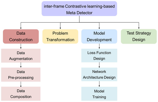
Figure 2.
The basic framework of the proposed method.
3.2. Data Construction
To study the problem of detecting targets in the presence of heterogeneous clutter, we assume that the narrow-band pulse Doppler radar under consideration transmits a coherent burst of M pulses. For the received signal in a dominant clutter background, the traditional RTD problem can be formulated as the binary hypothesis test:
where , , and denote the target vector, the clutter vector, and the noise vector, respectively. With frame (in this paper, a frame means a coherent pulse interval) receiving the raw data and each frame data covering range cells, the original dataset can be denoted as . is the received raw data in the -th range cell of the -th frame. Assuming that the target-present data are divided into classes and there are K-frame available target-absent data for each range cell (), the detection task for each range cell can be regarded as the i.i.d. N-way K-shot classification task in the signal domain, which satisfies the underlying assumption for meta-learning. Next, we prepare a dataset suitable for a meta-learning strategy through data augmentation, data pre-processing, and data composition.
3.2.1. Data Augmentation
In this part, we manually generate the target-present signal by adding the artificial moving target signal with random amplitudes and different velocities into the available target-absent signal to augment the training dataset. So, we assign different categories for target-present data with different target velocities. Specifically, the sample augmented by for the n-th class can be expressed as
where denotes the target echo simulated for the n-th kind of samples, and denotes its amplitude, calculated by SCNR randomly sampled from a preset range, which is assumed to vary negligibly during the coherent pulse interval (CPI). is the normalized Doppler frequency defined for the moving targets in the n-th class according to our label assignment rule introduced below.
In this paper, the labeling of data is related to the location of the radar target depicted in the Doppler spectrum. The Doppler spectrum is acquired through the discrete Fourier transform (DFT) operation. Assuming the number of discrete Fourier points is , we assign the label n to target-present data with velocities falling within the range , where . Here, denotes the velocity corresponding to the n-th discrete Doppler point. denotes the velocity whose value is equal to half of the velocity resolution of the radar system. To this end, the relation between and is
where is the wavelength, and is the pulse repetition frequency (PRF).
To facilitate the investigation of moving-target detection, we devise an adaptive strategy to define the velocity range of hard-to-detect targets under complex clutter backgrounds. Particularly, we determine the estimated noise power by selecting the highest noise power among Doppler channels within the noise zone. Doppler channels exhibiting power higher than this estimated noise power are identified as belonging to a strong clutter zone. The velocity range corresponding to these channels is then considered as hard to detect.
3.2.2. Data Pre-Processing
Given the crucial role of Doppler information in RTD, we have devised a data pre-processing module, as depicted in Figure 3, to extract abundant Doppler information from received echoes. To elaborate, we initially transmit the M-dimensional signal vector post-pulse compression (PC), such as in Figure 3, through an -point discrete Fourier transform of the coherent operator for yielding the -dimensional Doppler spectrum. Subsequently, we normalize the obtained Doppler spectrum to derive the CDI vector. Following this, we compute the DDI by normalizing the Doppler vector representing the deviation between the input signal vector and the target-absent signal from the previous frame but within the same range cell, exemplified by and illustrated in Figure 3. Eventually, we concatenate the CDI vector and the DDI vector as the Doppler feature vector for each received radar echo, such as in Figure 3. To this end, we obtain the dataset from the initial data , where denotes the label of When n equals N, the subset comprises target-absent Doppler feature vectors. Conversely, when n does not equal N, the subset comprises target-present Doppler feature vectors with the target Doppler of .
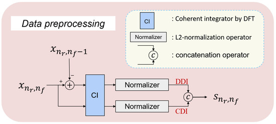
Figure 3.
Flow chart of data pre-processing.
3.2.3. Data Composition
Targets often experience range spreading due to data sampling or the target size exceeding the range resolution. Once range spreading occurs, the target energy spills into the adjacent range cell, leading to a degradation in target detection performance in conventional detectors. To address this issue, we concatenate the Doppler feature vectors of the CUT and its neighboring range cells, and treat the resulting vector as the representation sample for the CUT. Specifically, the Doppler feature vector of CUT is denoted as . In narrow-band radar systems with relatively low radar resolution, it is rarely possible for a point-like target to occupy more than two range cells. Consequently, the Doppler feature vectors of a left-adjacent range cell and a right-adjacent range cell, denoted as and , are enough to prevent the target energy loss. Meanwhile, considering the complex-value property of samples, the input sample matrix that we finally construct for our network can be denoted as
To this end, the finally constructed dataset for our model is denoted as
3.3. Problem Transformation
To summarize the preparation of samples and labels above, we independently tailor the RTD task for each range cell and transform it to an N-way K-shot classification task. First of all, following the episodic training strategy used by meta-learning methods, we treat the RTD task in each range cell as an episode and split data into the meta-train set and the meta-test set . Concretely, consists of the samples from the range cells for training and consists of the samples from the range cells for testing. Here, denotes the index set of range cells for training, denotes the index set of range cells for testing, and .
Secondly, according to the primary mechanism in few-shot learning, each N-way K-shot episode consists of the support set and the query set. Following this, for meta-training, we randomly sample K instances per class for all episodes in to obtain the support set . Similarly, we then sample instances per class to obtain the query set . Note that . , , and . Given the same operation for meta-testing on the dataset , we obtain the support set and query set . Denoting the lengths of and as and , respectively; is set equal to as well as K according to the custom of few-shot learning. In addition, for logical integrity, an extra constraint that is imposed in this paper. For ease of implementation, denoting the lengths of and as and , respectively, the aforementioned datasets can be simplified as
Here, is the i-th sample in the j-th episode of , and is the label of . Similarly, is the i-th sample in the j-th episode of , and is the label of . is the i-th sample in the j-th episode of , and is the label of . is the i-th sample in the j-th episode of , and is the label of . denotes the number of samples in each episode.
The datasets obtained previously will be utilized as follows: During the meta-training stage, we train our model using the dataset and . Then, the dataset is employed to fine-tune the network before the performance evaluation on the dataset . In this way, conventional radar target detection in a complex clutter environment is effectively transformed into an N-way K-shot problem, amenable to solutions based on meta-learning approaches.
3.4. Model Development
To address the limitation of model-specific methods and obtain the desired generalization capability, we develop a model-agnostic meta-detector via inter-frame CL. As shown in Figure 4, the proposed model is primarily implemented by the Siamese network architecture (framed in the pink rectangle) and optimized by the loss function (framed in the gold rectangle). The model development procedure involves two stages: the meta-training stage and the meta-testing stage. During the meta-training stage, pairs of samples in each episode are sent to the feature extractors with shared weights, which consist of an encoder and a projector [53,54,55,56,57,58]. Leveraging the introduced training paradigm of meta-learning, the parameters of the network are updated by back-propagating the gradient from the designed loss function. During the meta-testing stage, the network is first fine-tuned using the support set of the target task. Subsequently, with the optimized encoder and the devised test module (framed in the green rectangle in Figure 4), it can be efficiently determined whether the sample under testing contains a moving target or not. In the following discussion, we delve into the specifics of our loss function, network architecture, and model training procedure.
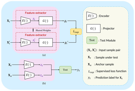
Figure 4.
The overview of the proposed detector. (a) Training. (b) Testing.
3.4.1. Loss Function Design
Recently, contrastive loss has become prevalent due to its inherent property of being hardness-aware. Since samples containing weak targets and target-absent samples can be viewed as hard negative samples of each other, selecting an appropriate contrastive loss is crucial for our task. However, the conventional CL literature typically forms negative pairs by randomly selecting samples from the mini-batch, which makes it possible to pull a pair of samples in the same class away by mistake. In addition, the conventional CL’s self-supervised nature makes it impossible to fully utilize the supervision information of our dataset. Given this issue, we adopt a supervised contrastive loss [32] to leverage the label information and improve the contrastive power with accurate negative pairs. Specifically, for the N-way K-shot problem, the supervised contrastive loss is formulated as
Here, is the index of the i-th sample, denoted as , in an episode. is the index of positive samples constructed for , denoted as . and are labels of and , respectively. is its cardinality. and are the output vectors of and , respectively, after the feature extractor. is the index of the other samples in the same episode as , denoted as . is the label of . is an adjustable temperature scalar. denotes the cosine function, i.e.,
The operation denotes the inner-dot product.
To understand the hardness-aware property of the supervised loss function, we consider the loss for the positive pair , i.e.,
Obviously, the relation between Equation (13) and Equation (11) can be expressed as
Denoting the cosine similarity of the positive pair as , the gradient of Equation (11) with respect to is formulated as
where B is a scalar independent with :
Similarly, consider the loss for the negative pair , the gradient of Equation (11) with respect to the cosine similarity is formulated as
where F is a scalar independent with :
From Equation (15), we conclude that the decreased gradient back-propagated by the supervised loss function will be larger for hard positive pairs than normal positive pairs, aiming to pull the hard positive pair closer in the feature space. Similarly, from Equation (17), the decreased gradient back-propagated by the supervised loss function will also be larger for hard negative pairs than normal negative pairs, to push the hard positive pair further in the feature space. Consequently, in our model, the supervised loss function in Equation (11) will significantly promote learning for the hard-to-detect targets and the clutter.
3.4.2. Network Architecture Design
We exhibit the network architecture of the feature extractor, including an encoder and a projector , in Figure 5. Concretely, as shown in Figure 5a, the encoder contains a convolution followed by a ReLU non-linearity layer [59], a convolution, a ReLU non-linearity layer, and a average-pooling layer. The non-linear activation function ReLU(·) is defined as
Moreover, we construct the projector with a multi-layer perceptron (MLP), as shown in Figure 5b. Noticeably, following the common practice in CL to improve the performance on downstream tasks, we discard the projector at the end of training [58]. As a result, the output representations of the optimized encoder are directly utilized during testing.
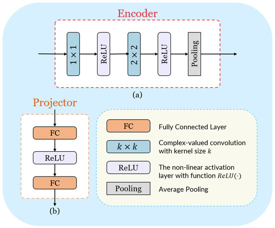
Figure 5.
The network architecture of the feature extractor in Figure 4. (a) The network architecture of the encoder. (b) The network architecture of the projector.
3.4.3. Model Training
In this paper, the training of our model comprises two parts, the meta-training stage and the fine-tuning stage, before performance evaluation during the meta-testing stage. During the meta-training stage, we adopt the optimization strategy in model-agnostic meta-learning (MAML) [39,60]. This strategy initializes the model and allows it to adapt efficiently to the new task. For the fine-tuning stage, the model is further optimized on the support set of the target task. In other words, the model is equipped with the across-task knowledge during the meta-training stage and the task-specific knowledge during the fine-tuning stage. Algorithm 1 summarizes the complete meta-learning framework fitting for both the meta-training and the fine-tuning.
| Algorithm 1 Model Training Algorithm for IfCMD |
|
After fine-tuning, as depicted in Figure 4b, the encoded representations of samples in the query set of the target task are sent into the test module to predict the labels. Below, we describe the details of the detection strategy in the test module.
3.5. Test Strategy Design
Inspired by the fact that the inter-frame information changes differently for a range cell with or without the target, we devised our “test” module to detect targets based on the cosine similarity between sample pairs in the feature space. To begin with, denoting the encoded representations of a sample pair as and , respectively, the PDF of the cosine similarity between the representation pair can be expressed as , where . Since the change information is the crucial goal, an identified target-absent sample is randomly selected from each task in the dataset as the anchor sample for that task when estimating the PDF. As a result, the binary hypothesis for our detection problem can be formulated as and . Since the label of the anchor sample is known in advance, and can be regarded as other forms of and . At the end of the meta-training procedure in Algorithm 1, the PDF of cosine similarity between positive pairs constructed by target-absent samples, i.e., , can be estimated on the dataset . Since can be approximated as a Gaussian distribution based on experimentally fitted density curves, the detection threshold can be calculated with and the preset constant Pfa.
At test time, denoting the sample in the CUT as and its corresponding anchor sample as , the cosine similarity between the representation vectors of and is expressed as . To this end, the decision on whether the CUT contains a target is efficiently made by comparing and the detection threshold . This allows the proposed detector’s performance to be assessed under the CFAR condition and compared with traditional detectors. The intuitive illustration of the test module is shown in Figure 6.
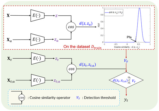
Figure 6.
The intuitive illustration of the test module.
4. Experimental Results
In this section, we will test the proposed method on the simulated dataset to demonstrate its effectiveness. We first introduce the experimental settings, including the simulated dataset, implementation details, compared methods, and evaluation metrics. Then, under these settings, we evaluate the detection performance and generalization ability of the proposed method. Finally, we present qualitative analysis and computational analysis for our method.
4.1. Experimental Settings
4.1.1. Dataset Description
For our experiments, the simulated dataset is considered as the received data of a narrow-band ground-based warning radar. The parameters of the radar system are shown in Table 1. To verify the effectiveness of IfCMD under a complex dynamic clutter background, we construct an experimental environment containing four types of clutter with different motion states. Specifically, the first type of clutter background, called Clutter I, is static clutter with an average clutter-to-noise ratio (CNR) of 55 dB, zero speed, and an almost negligible standard derivation (std) of the speed. Differently, we set the second type of clutter background, Clutter II, as the representative of dynamic clutter with a non-zero Doppler frequency. The third type of clutter background, Clutter III, is designed to represent dynamic clutter with Doppler spectral broadening. To explore the performance gain near the non-homogeneous clutter edge, we set the average CNR of Clutter II and Clutter III to 50 dB and 60 dB, respectively. Furthermore, to evaluate the generalization performance of IfCMD, Clutter IV is simulated as a combination of Clutter II and Clutter III, but with totally different CNR and velocity parameters. In summary, the parameters of four types of clutter are depicted in Table 2, and the characteristics of the simulated data are displayed in Figure 7.

Table 1.
The parameters of the narrow-band ground-based surveillance radar system.
Table 2.
Parameters of the four types of clutter.
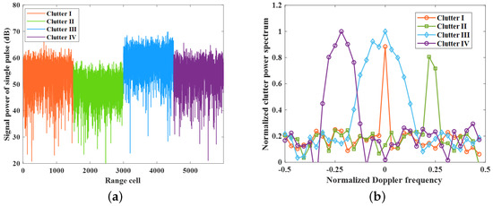
Figure 7.
Characteristics of the simulated data. (a) The distribution of the four types of clutter along the range. (b) The Doppler characteristics of the four types of clutter.
This paper primarily focuses on investigating the moving-target detection performance of the proposed method in dynamic clutter environments and near non-homogeneous clutter edges, where conventional RTD methods suffer from severe performance loss in both conditions. To conduct our experiments, the simulated dataset is utilized as follows:
- Since Clutter I is the static clutter background causing little performance loss in traditional RTD methods, the RTD tasks of all range cells in Clutter I are used to train the model.
- We randomly select 80% of the tasks from Clutter II and Clutter III for meta-training, while the remaining 20% are used for performance evaluation.
- To enhance the generalization ability of the trained model, we employ 9-fold cross-validation during training to tune the parameters.
- Finally, all tasks of Clutter IV are reserved for the generalization performance test.
4.1.2. Implementation Details
The implementation details contain two parts: the hyper-parameter selection and the hardware settings. We summarize the settings for hyper-parameters in Table 3. Specifically, we set the number of DFT points to 32, which is equal to the number of pulses in a CPI. As a result, N equals 33, transforming the target detection task into a 33-way few-shot classification problem. Following the data construction strategy outlined in Section 3, we simulate the required target-present samples and assign labels accordingly. The SCNR range for targets is set as [—20 dB, 20 dB] based on practical experience. With the above settings, we simulate 50 frames of data, including both target-absent samples and target-present samples, where the simulated targets obeys the Swerling type-0/5 fluctuation. The number of samples in each category of the episode is set as 25, i.e., . In addition, hyper-parameters for optimization, such as the learning rate and the meta-learning rate in Algorithm 1, are tuned through the 9-fold cross-validation, with the final selection also presented in Table 3. As for hardware settings, we implement our model on a 3.2 GHz CPU and run our experiment on an NVIDIA GeForce GTX 1080 GPU (NVIDIA, Santa Clara, CA, USA) in the PyTorch framework. The Adam optimizer is utilized to optimize our model.
Table 3.
The settings for hyper-parameters.
4.1.3. Compared Methods
To demonstrate the effectiveness of our method, we compare it with five classical RTD methods, including cell-averaging CFAR (CA-CFAR) in the Doppler domain, MTI followed by MTD and CA-CFAR (MTI-MTD), the generalized likelihood ratio test (GLRT), clutter map (CM) [61], and the adaptive normalized matched filter (ANMF) [62]. We choose these five methods as comparison methods for the following reasons:
- CA-CFAR: a kind of CFAR detector that is widely explored in both theoretical analysis and realistic applications for RTD tasks.
- MTI-MTD: a conventional processing flow for target detection in clutter environments.
- GLRT: the representative of the likelihood ratio test (LRT) algorithm for RTD in a clutter background.
- CM: a popular non-coherent RTD method involving multi-frame data processing.
- ANMF: a novel adaptive filter for RTD in low-rank Gaussian clutter.
4.1.4. Evaluation Metrics
Since the novel detection strategy proposed in this paper can estimate the detection threshold in the latent space mapped by the encoder, we follow the traditional RTD evaluation metric, i.e., the probability of detection (PD) under the constant Pfa. Therefore, in order to intuitively demonstrate the effectiveness of the proposed method, we provide the curves of PD versus SCNR after coherent integration to depict the detection performance for targets whose Doppler is located in the clutter region.
4.2. Detection Performance and Comparisons
In this section, numerical results on simulated data are presented to show the detection performance of the proposed method. Specifically, we evaluated the target detection performance of IfCMD under the Clutter II and Clutter III backgrounds, respectively, to verify its robustness against dynamic clutter backgrounds. In addition, given that a prominent feature of our approach is its immunity to the clutter edge effect, we also statistically analyzed the detection performance of IfCMD for targets appearing near the edges of Clutter II and Clutter III to validate that. Finally, we evaluated the detection performance of all compared methods for range-spread targets. Note that the desired Pfa used to calculate the detection threshold in the compared methods is set as 1 × 10⁻⁶. For fair comparison, the number of Monte Carlo (MC) trials is set as .
4.2.1. Detection Performance for Targets under a Dynamic Clutter Background
On the one hand, to verify the robustness of the proposed method in a dynamic clutter background with non-zero velocity mean, we compare the target detection performance of all the methods under the Clutter II background in Figure 8. The curves of PD versus normalized Doppler frequency with an SCNR of 6 dB are displayed in Figure 8a. Since the normalized Doppler frequency of Clutter II is about 0.22, all methods suffer detection performance degradation for targets whose normalized Doppler frequency is close to the normalized Doppler frequency of Clutter II. Additionally, MTI-MTD also experiences a loss in detection performance for targets with Doppler close to zero, attributed to the presence of the extremely deep notch near zero frequency [27]. To further explore the detection performance of the proposed method for targets with velocities close to the clutter, we show the PD curves of all the methods for targets with normalized Doppler frequencies of 0.22 and 0.25 in Figure 8b and Figure 8c, respectively. For targets with a normalized Doppler frequency of 0.22, given the detection probability PD = 0.6, the required SCNR of IfCMD is about 1.8 dB higher than MTI-MTD and CA-CFAR. GLRT and ANMF are invalid for such hard-to-detect targets with almost zero velocity relative to the clutter. In essence, the algorithms of GLRT and ANMF are akin to forming extremely deep notches in the vicinity of the Doppler where the clutter is located. However, due to the insufficiently precise notch, the detection performance of GLRT and ANMF for targets whose Doppler is within the notch’s coverage is poor. As for CM, which detects targets in the time domain, the SCNR of targets is small due to the lack of coherent integration. Therefore, the target detection performance of CM is not satisfactory. For targets with a normalized Doppler frequency of 0.25, given the detection probability PD = 0.8, the required SCNR of IfCMD is about 2 dB higher than MTI-MTD and CA-CFAR. GLRT and ANMF remain ineffective in addition to CM.
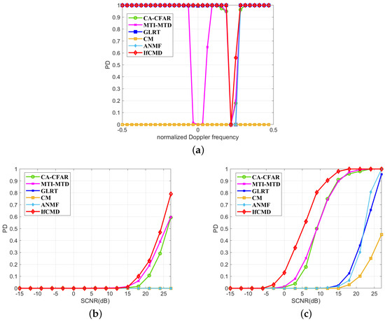
Figure 8.
Moving-target detection performance under Clutter II background. (Pfa = 1 × 10⁻⁶). (a) Curves of PD versus normalized Doppler frequency (SCNR = 6 dB). (b) Curves of PD versus SCNR ( = 0.22). (c) Curves of PD versus SCNR ( = 0.25). denotes the mean of normalized Doppler frequencies of targets under test.
On the other hand, to validate the effectiveness of the proposed method against dynamic clutter backgrounds characterized by Doppler spectral broadening, we compare the target detection performance of all the methods under the Clutter III background. Similar to the study for Clutter II, the curves of PD versus normalized Doppler frequency with SCNR of 6 dB are first displayed in Figure 9a. Due to the Doppler broadening, the Doppler range of undetectable targets in the Clutter III background is wider than that in the Clutter II background. According to Figure 9a, the broadening Doppler spectrum greatly hinders the target detection of traditional RTD methods, especially for GLRT, ANMF, and CM. To further explore the detection performance of the proposed method for hard-to-detect targets, we show the PD curves of all the methods for targets with normalized Doppler frequencies of —0.06, —0.03, 0, and 0.03 in Figure 9b–Figure 9e, respectively. For targets with a normalized Doppler frequency of —0.06, corresponding to a velocity of —3.13 m/s in Figure 9b, given the detection probability PD = 0.8, the required SCNR of IfCMD is about 2.8 dB higher than MTI-MTD and CA-CFAR. For targets with a normalized Doppler frequency of —0.03, corresponding to a velocity of —1.56 m/s, in Figure 9c, given the detection probability PD = 0.8, the required SCNR of IfCMD is about 3 dB and 3.8 dB higher than CA-CFAR and MTI-MTD, respectively. For targets with a normalized Doppler frequency of 0.03, corresponding to a velocity of 1.56 m/s, in Figure 9e, given the detection probability PD = 0.8, the required SCNR of IfCMD is about 3.9 dB and 4.5 dB higher than CA-CFAR and MTI-MTD, respectively. All methods suffer severe performance degradation for the target with a mean velocity of 0 m/s in Figure 9d, but IfCMD still achieves the highest PD compared with others. In Figure 9b–e, GLRT, ANMF, and CM remain unsatisfactory for such targets. In addition, due to the extremely deep notch near zero frequency, when the target velocity approaches zero, the detection performance of MTI-MTD degrades more, even lower than that of CA-CFAR.
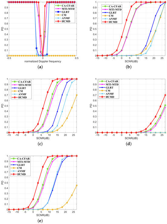
Figure 9.
Moving-target detection performance under Clutter III background (Pfa = 1 × 10⁻⁶). (a) Curves of PD versus normalized Doppler frequency (SCNR = 6 dB). (b) Curves of PD versus SCNR ( = —0.06). (c) Curves of PD versus SCNR ( = —0.03). (d) Curves of PD versus SCNR ( = 0). (e) Curves of PD versus SCNR ( = 0.03). denotes the mean of normalized Doppler frequencies of targets under test.
In summary, IfCMD performs well in dealing with the RTD problem in a dynamic clutter background in the cases of both non-zero clutter velocities and severe broadening of the clutter spectrum.
4.2.2. Detection Performance for Targets near the Clutter Edge
In order to demonstrate the insensitivity of the proposed method to clutter edge effects, we show the target detection performance of the clutter edge for Clutter II and Clutter III in Figure 10. Firstly, we exhibit the detection performance of CUTs of Clutter II affected by reference cells in Clutter III in Figure 10a. Compared with the results in Figure 8a, traditional methods, including CA-CFAR, GLRT, and ANMF, suffer serious performance degradation for targets whose velocity approaches the velocity of Clutter III. Similarly, we exhibit the detection performance of CUTs of Clutter III affected by range cells in Clutter II in Figure 10b. Comparing the results in Figure 10b with Figure 9a, we find the same phenomenon with the comparison between Figure 8a and Figure 10a. This is because these traditional methods model the clutter in the CUT with its surrounding range cells. As a result, they are vulnerable to the clutter edge effect. Unlike traditional methods, IfCMD is robust to the clutter edge effect and achieves the best detection performance among comparison methods due to the independent treatment of each range cell.
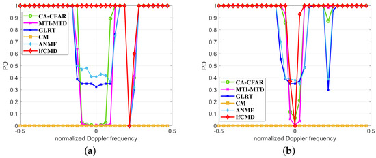
Figure 10.
Detection performance for targets near the clutter edges of Clutter II and Clutter III (Pfa = 1 × 10⁻⁶, SCNR = 6 dB). (a) Detection performance for CUTs of Clutter II affected by Clutter III. (b) Detection performance for CUTs of Clutter III affected by Clutter II.
4.2.3. Detection Performance for Range-Spread Targets
While narrow-band radar targets are usually modeled as point targets in practical scenarios, some targets may range-extend in a small number of distance cells because of unexpected factors such as data oversampling. Here, the detection performance of range-spread targets is evaluated among all compared methods. Considering that the scale of moving targets will not be more than twice the range resolution simulated in this paper, we set the number of adjacent range cells with the target spreading as two. To highlight the range-spread problem, the power distributed in each spread cell is set as half of the total target energy.
In Figure 11 and Figure 12, we display the range-spread-target detection performance of all the methods in Clutter II and Clutter III backgrounds. Specifically, we provide an overview of the detection performance of all the methods for range-spread targets with different normalized Doppler frequencies but the same SCNR of 6 dB in Figure 11a and Figure 12a. For intuitive comparison, we plot the detection curves of each method for targets with and without range spreading in the same subfigure and distinguish them with the suffix “-w” in the legend, as shown in Figure 11b–e and Figure 12b–e. It is well established that traditional methods invariably suffer significant performance degradation when confronted with range-spread targets. As an example, for targets with the normalized Doppler frequency of 0.25 in the Clutter II background, we observe results in Figure 11d,e and find that all the compared traditional methods suffer an average performance loss of about 2∼3 dB. However, IfCMD remains unaffected by range spreading, maintaining consistent performance regardless of the presence of range spread. This resilience is attributed to the design of the sample composition, where we incorporate information from nearest-neighbor range cells into the CUT and utilize a convolutional neural network with spatial translation invariance to extract this information. The same phenomenon appears in Figure 12a–e. To this end, the proposed method, equipped with efficient measures to address the range-spread-target detection problem, demonstrates remarkable robustness against such targets. In Figure 11 and Figure 12, we present the range-spread-target detection performance of all methods in Clutter II and Clutter III backgrounds.
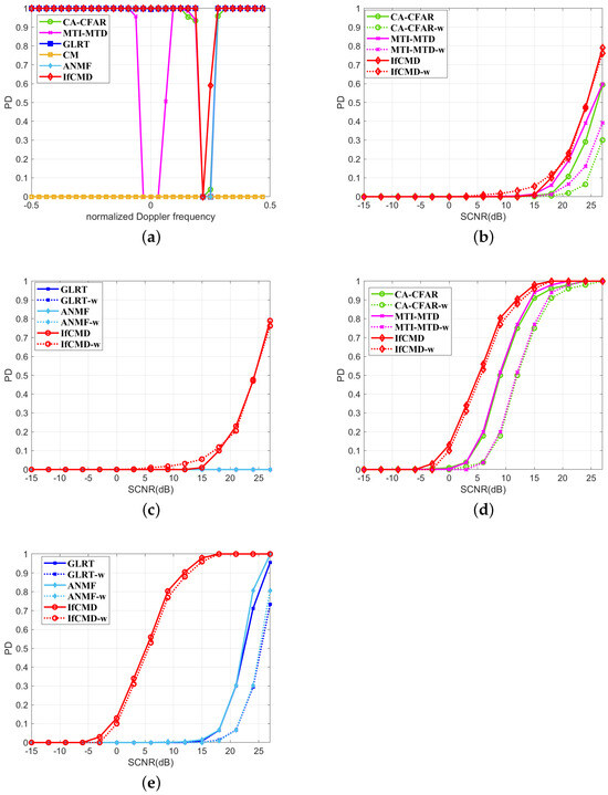
Figure 11.
Range-spread-targetdetection performance for Clutter II (Pfa = 1 × 10⁻⁶). (a) Curves of PD versus normalized Doppler frequency (SCNR = 6 dB). (b) Performance comparison with CA-CFAR and MTI-MTD (). (c) Performance comparison with GLRT and ANMF (). (d) Performance comparison with CA-CFAR and MTI-MTD (). (e) Performance comparison with GLRT and ANMF (). To differentiate, the curves with the suffix “-w” in the legend are detection results for range-spread targets.
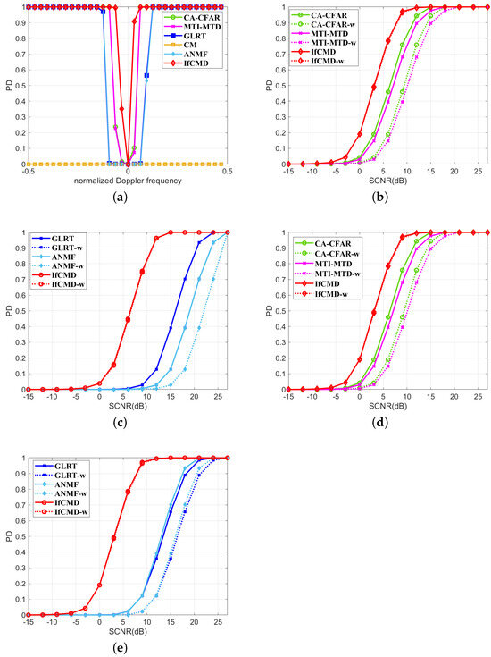
Figure 12.
Range-spread-targetdetection performance for Clutter III (Pfa: 1 × 10⁻⁶). (a) Curves of PD versus normalized Doppler frequency (SCNR = 6 dB). (b) Performance comparison with CA-CFAR and MTI-MTD (). (c) Performance comparison with GLRT and ANMF (). (d) Performance comparison with CA-CFAR and MTI-MTD (). (e) Performance comparison with GLRT and ANMF (). To differentiate, the curves with the suffix “-w” in the legend are detection results for range-spread targets.
4.3. Generalization Performance Analysis
To demonstrate the generalization ability of IfCMD, we test it under the background of Clutter IV, which is the new task for the proposed model after meta-training. After fine-tuning the model with 25 frames of simulated data of the target task, the moving-target detection performance in the Clutter IV background is evaluated and shown in Figure 13.
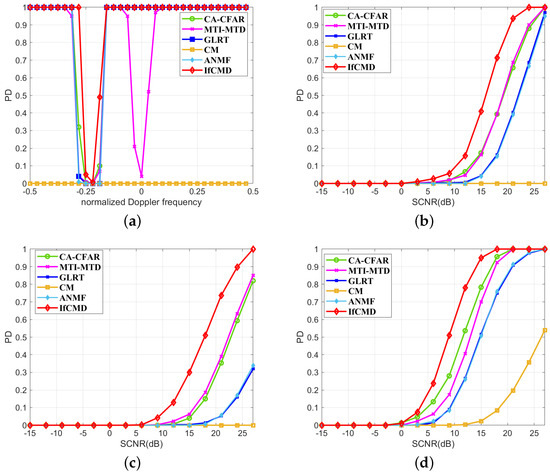
Figure 13.
Moving-target detection performance for Clutter IV (Pfa = 1 × 10⁻⁶). (a) Curves of PD versus normalized Doppler frequency (SCNR = 6 dB). (b) Curves of PD versus SCNR ( = —0.25). (c) Curves of PD versus SCNR ( = —0.22). (d) Curves of PD versus SCNR ( = —0.19).
Specifically, we first display plots of all the methods for targets with different Doppler frequencies but the same SCNR of 6 dB in Figure 13a. To further explore the detection performance for targets with Doppler frequencies close to —0.22 (the Doppler frequency of the main clutter in the Clutter IV background), we show the PD curves of all the methods for targets with normalized Doppler frequencies of —0.25, —0.22, and —0.19 in Figure 13b–Figure 13d, respectively. For targets with normalized Doppler frequencies of —0.25, —0.22, and —0.19, given the detection probability of 0.8, the required SCNR of IfCMD is about 3.2 dB, 4 dB, and 2.8 dB lower than the required SCNR of the best traditional method, respectively.
Consequently, even for a completely unseen environment, IfCMD can finish the moving-target detection task well with only a few data for model optimization.
4.4. Qualitative Analysis
Apart from the quantitative evaluation above, we also make some qualitative analysis in this section to further illustrate the efficiency of our model. In this paper, rather than concentrating solely on instance-level features, our model dynamically makes decisions based on pairwise sample similarities in the latent space. Consequently, we provide a qualitative analysis from the perspective of the statistical characteristics of pairwise sample similarities in the latent space. As a representative example, the target velocity of the target-present samples used to characterize statistics here is set as 3.13 m/s, and the target-absent samples used here are in the Clutter III background.
As depicted in Figure 14, we explore the effect that our model imposes on the targets with different SCNRs. In the second column of Figure 14, we show and for different SCNRs. For intuitive comparison, two PDFs of the test statistic under the binary hypothesis derived by traditional likelihood ratio test (LRT) theory are shown in the first column of Figure 14. denotes the normalized module of the signal here.
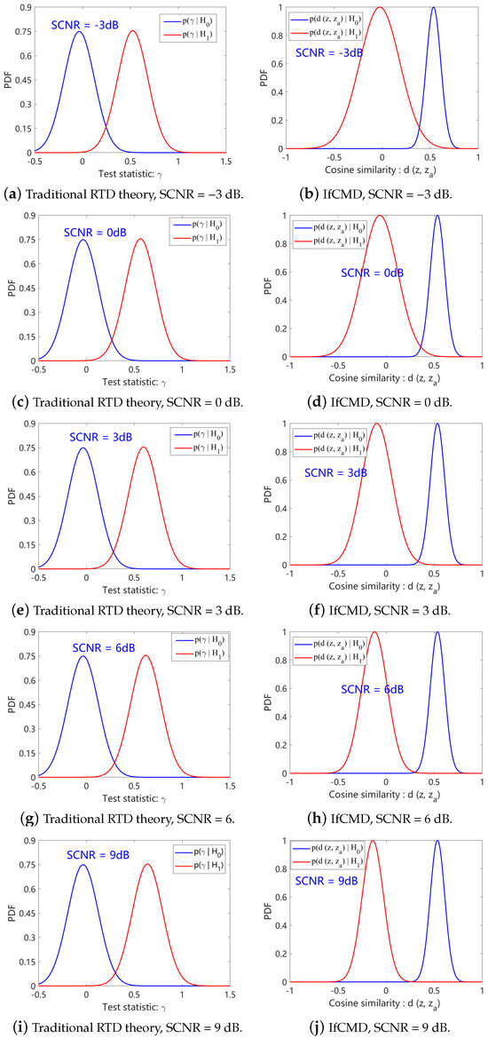
Figure 14.
Qualitative analysis under Clutter III background. The target velocity is 3.13 m/s.
According to Figure 14, the following observations can be obtained:
- Traditional RTD theory assumes that the difference between the statistical properties of target-present and target-absent signals is reflected in the mean rather than the variance. The mean difference between and amplifies as the SCNR increases.
- Different from traditional RTD theory, in the latent space of our optimized model, the differences between the statistical properties of target-present signals and target-absent signals are reflected in both the mean and the variance. As the SCNR increases, the differences of both the mean and the variance between and amplify.
Incorporating these observations, we conclude that our model is devoted to aggregating each class of samples into a tighter cluster while keeping the cluster of target-present samples further from the cluster of target-absent samples.
4.5. Computational Analysis
A computational comparison between all the methods is presented in this part. Since the dimension of the latent layer in our networks is equal and denoted as , the computational complexity of IfCMD can be calculated by the following expression:
Consequently, the computational load of IfCMD is , indicating that the computational load of IfCMD does not significantly increase with the degrees of freedom of radar systems. In addition, we display the time cost for one CUT among all the comparison methods in Table 4. Specifically, GLRT and ANMF requires a lot of time for each time of test due to involving the inverse operation of the clutter covariance matrix. Compared with them, CA-CFAR, MTI-MTD, and CM require much less time. IfCMD is trained offline, and then, fine-tuned online before testing, and the range cells can be processed in parallel, so IfCMD is efficient during the testing phase. To this end, the offline training and the parallel testing equip our method with the capability of real-time testing.
Table 4.
The time cost for one CUT.
5. Measured Results
In this section, we present the target detection performance of IfCMD on measured data. The parameters of the radar system used for the measured data are shown in Table 5. In addition, we utilize an unmanned aerial vehicle (UAV) as a moving target to acquire a real-world target-present signal, and the velocity of the UAV is set as 2 m/s. The range-Doppler spectrum of measured data in a randomly selected frame is shown in Figure 15a, and the Doppler spectrum of radar echo in the target-present range cell is shown in Figure 15b. As depicted in Figure 15, the moving target is coupling with clutter and extended in both the distance and Doppler dimensions. This fact renders targets hard to detect in traditional RTD methods. To evaluate the performance of compared methods, we calculate the PD for detection results of target-present CUTs in 20,000 consecutive frames of radar echos for each compared method and list them in Table 6. As shown in Table 6, our method achieves the best performance among compared methods on measured data, which is consistent with the results in Section 4 and demonstrates the effectiveness of IfCMD again.
Table 5.
Parameters of radar system for measured data.
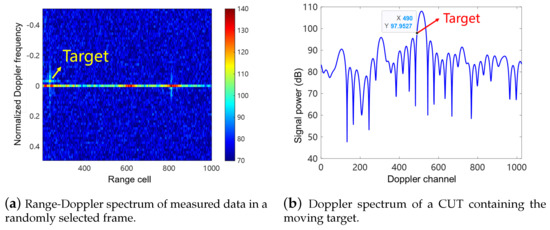
Figure 15.
Characteristics of moving targets with velocity of 2 m/s for measured data.
Table 6.
Quantification analysis for measured data.
6. Discussion
This paper aims to enhance detection performance for moving targets, especially for targets that are hard to detect for traditional RTD methods, in complex clutter environments using DL-based methods. Inspired by its effectiveness, we aim to explore promising directions for addressing other challenging issues in RTD, such as highly maneuvering target detection and adaptive detection of range-spread targets in clutter environments, in the future.
7. Conclusions
In this paper, we propose a novel data-driven detector, called IfCMD, to improve the detection performance of moving targets in complex clutter environments. By recasting the traditional RTD task into a few-shot classification problem, we draw from the concept of contrastive learning and treat hard-to-detect targets as hard negative samples to clutter. Accordingly, we develop our model based on the Siamese network architecture, which is optimized with a supervised contrastive loss, guiding the model to push hard negative samples away from each other in the feature space. Additionally, we employ the meta-learning strategy to endow our model with the capability of generalizing to new tasks efficiently. Finally, we design a straightforward yet powerful test module to ensure the end-to-end implementation of our detector. Our approach shows appealing properties that can overcome several shortcomings of traditional RTD methods. Extensive experiments have been carried out, demonstrating that our method achieves consistent performance improvements in detecting targets under complex clutter environments and generalizing to new RTD tasks with only a few labeled data.
Author Contributions
Conceptualization, H.L. and B.C.; methodology, C.Z.; software, C.G. and C.Z.; validation, W.C. and C.Z.; formal analysis, Y.X. and C.Z.; investigation, C.Z.; resources, H.L.; data curation, C.G.; writing—original draft preparation, C.Z.; writing—review and editing, C.Z. and Y.X.; visualization, C.Z. and Y.X.; supervision, C.Z. and Y.X.; project administration, B.C. and W.C.; funding acquisition, B.C. and W.C. All authors have read and agreed to the published version of the manuscript.
Funding
This work was supported in part by the National Natural Science Foundation of China under Grant U21B2006; in part by Shaanxi Youth Innovation Team Project; in part by the 111 Project under Grant B18039; in part by the Fundamental Research Funds for the Central Universities QTZX23037 and QTZX22160.
Institutional Review Board Statement
Not applicable.
Informed Consent Statement
Not applicable.
Data Availability Statement
No new data were created or analyzed in this study. Data sharing is not applicable to this article.
Conflicts of Interest
The authors declare no conflicts of interest.
Abbreviations
The following abbreviations are used in this manuscript:
| CL | Contrastive learning |
| CFAR | Constant false alarm rate |
| CUT | Cell under test |
| CCM | Clutter covariance matrix |
| CDI | Complete Doppler information |
| CI | Coherent integration |
| CA-CFAR | Cell-averaging CFAR |
| CPI | Coherent pulse interval |
| CNR | Clutter-to-noise ratio |
| DL | Deep learning |
| DDI | Differential Doppler information |
| DFT | Discrete Fourier transform |
| GLRT | Generalized likelihood ratio test |
| i.i.d. | Independent and identically distributed |
| IfCMD | Inter-Frame Contrastive Learning-Based Meta Detector |
| LRT | Likelihood ratio test |
| MTI | Moving-target indication |
| MTD | Moving-target detection |
| Probability density function | |
| Pfa | The probability of false alarm |
| PD | The probability of detection |
| RCS | Radar cross-section |
| RTD | Radar target detection |
| std | Standard derivation |
| SCNR | Signal-to-clutter plus noise ratio |
| SNR | Signal-to-noise ratio |
References
- Liu, W.; Liu, J.; Hao, C.; Gao, Y.; Wang, Y.L. Multichannel adaptive signal detection: Basic theory and literature review. Sci. China Inf. Sci. 2022, 65, 121301. [Google Scholar] [CrossRef]
- Sun, H.; Oh, B.S.; Guo, X.; Lin, Z. Improving the Doppler resolution of ground-based surveillance radar for drone detection. IEEE Trans. Aerosp. Electron. Syst. 2019, 55, 3667–3673. [Google Scholar] [CrossRef]
- Brennan, L.; Mallett, J.; Reed, I. Adaptive arrays in airborne MTI radar. IEEE Trans. Antennas Propag. 1976, 24, 607–615. [Google Scholar] [CrossRef]
- Ash, M.; Ritchie, M.; Chetty, K. On the application of digital moving target indication techniques to short-range FMCW radar data. IEEE Sens. J. 2018, 18, 4167–4175. [Google Scholar] [CrossRef]
- Matsunami, I.; Kajiwara, A. Clutter suppression scheme for vehicle radar. In Proceedings of the 2010 IEEE Radio and Wireless Symposium (RWS), New Orleans, LA, USA, 10–14 January 2010; pp. 320–323. [Google Scholar]
- Shrader, W.W.; Gregers-Hansen, V. MTI radar. In Radar Handbook; Citeseer: Princeton, NJ, USA, 1970; Volume 2, pp. 15–24. [Google Scholar]
- Navas, R.E.; Cuppens, F.; Cuppens, N.B.; Toutain, L.; Papadopoulos, G.Z. Mtd, where art thou? A systematic review of moving target defense techniques for iot. IEEE Internet Things J. 2020, 8, 7818–7832. [Google Scholar] [CrossRef]
- Jia, F.; Tan, J.; Lu, X.; Qian, J. Radar Timing Range–Doppler Spectral Target Detection Based on Attention ConvLSTM in Traffic Scenes. Remote Sens. 2023, 15, 4150. [Google Scholar] [CrossRef]
- Jalil, A.; Yousaf, H.; Baig, M.I. Analysis of CFAR techniques. In Proceedings of the 2016 13th International Bhurban Conference on Applied Sciences and Technology (IBCAST), Islamabad, Pakistan, 12–16 January 2016; pp. 654–659. [Google Scholar]
- Rohling, H. Ordered statistic CFAR technique—An overview. In Proceedings of the 2011 12th International Radar Symposium (IRS), Leipzig, Germany, 7–9 September 2011; pp. 631–638. [Google Scholar]
- Ravid, R.; Levanon, N. Maximum-likelihood CFAR for Weibull background. IEE Proc. F Radar Signal Process. 1992, 139, 256–264. [Google Scholar] [CrossRef]
- Qin, T.; Wang, Z.; Huang, Y.; Xie, Z. Adaptive CFAR detector based on CA/GO/OS three-dimensional fusion. In Proceedings of the Fifteenth International Conference on Signal Processing Systems (ICSPS 2023), Xi’an, China, 17–19 November 2024; Volume 13091, pp. 302–310. [Google Scholar]
- Rihan, M.Y.; Nossair, Z.B.; Mubarak, R.I. An improved CFAR algorithm for multiple environmental conditions. Signal Image Video Process. 2024, 18, 3383–3393. [Google Scholar] [CrossRef]
- Chalise, B.K.; Wagner, K.T. Distributed GLRT-based detection of target in SIRP clutter and noise. In Proceedings of the 2021 IEEE Radar Conference (RadarConf21), Atlanta, GA, USA, 7–14 May 2021; pp. 1–6. [Google Scholar]
- Shuai, X.; Kong, L.; Yang, J. Performance analysis of GLRT-based adaptive detector for distributed targets in compound-Gaussian clutter. Signal Process. 2010, 90, 16–23. [Google Scholar] [CrossRef]
- Kelly, E.J. An adaptive detection algorithm. IEEE Trans. Aerosp. Electron. Syst. 1986, AES-22, 115–127. [Google Scholar] [CrossRef]
- Robey, F.C.; Fuhrmann, D.R.; Kelly, E.J.; Nitzberg, R. A CFAR adaptive matched filter detector. IEEE Trans. Aerosp. Electron. Syst. 1992, 28, 208–216. [Google Scholar] [CrossRef]
- Fan, Y.; Shi, X. Wald, QLR, and score tests when parameters are subject to linear inequality constraints. J. Econom. 2023, 235, 2005–2026. [Google Scholar] [CrossRef]
- Wang, Z.; Chen, H.; Li, Y.; Wang, D. Rao and Wald Tests for Moving Target Detection in Forward Scatter Radar. Remote Sens. 2024, 16, 211. [Google Scholar] [CrossRef]
- LeCun, Y.; Bengio, Y.; Hinton, G. Deep learning. Nature 2015, 521, 436–444. [Google Scholar] [CrossRef] [PubMed]
- Wu, Z.; Wang, W.; Peng, Y. Deep learning-based uav detection in the low altitude clutter background. arXiv 2022, arXiv:2202.12053. [Google Scholar]
- Sun, H.H.; Cheng, W.; Fan, Z. Clutter Removal in Ground-Penetrating Radar Images Using Deep Neural Networks. In Proceedings of the 2022 International Symposium on Antennas and Propagation (ISAP), Sydney, Australia, 31 October–3 November 2022; pp. 17–18. [Google Scholar]
- Si, L.; Li, G.; Zheng, C.; Xu, F. Self-supervised Representation Learning for the Object Detection of Marine Radar. In Proceedings of the 8th International Conference on Computing and Artificial Intelligence, Tianjin, China, 18–21 March 2022; pp. 751–760. [Google Scholar]
- Coiras, E.; Mignotte, P.Y.; Petillot, Y.; Bell, J.; Lebart, K. Supervised target detection and classification by training on augmented reality data. IET Radar Sonar Navig. 2007, 1, 83–90. [Google Scholar] [CrossRef]
- Jiang, W.; Ren, Y.; Liu, Y.; Leng, J. A method of radar target detection based on convolutional neural network. Neural Comput. Appl. 2021, 33, 9835–9847. [Google Scholar] [CrossRef]
- Yavuz, F. Radar target detection with CNN. In Proceedings of the 2021 29th European Signal Processing Conference (EUSIPCO), Dublin, Ireland, 23–27 August 2021; pp. 1581–1585. [Google Scholar]
- Liang, X.; Chen, B.; Chen, W.; Wang, P.; Liu, H. Unsupervised radar target detection under complex clutter background based on mixture variational autoencoder. Remote Sens. 2022, 14, 4449. [Google Scholar] [CrossRef]
- Deng, H.; Clausi, D.A. Unsupervised segmentation of synthetic aperture radar sea ice imagery using a novel Markov random field model. IEEE Trans. Geosci. Remote Sens. 2005, 43, 528–538. [Google Scholar] [CrossRef]
- Le-Khac, P.H.; Healy, G.; Smeaton, A.F. Contrastive representation learning: A framework and review. IEEE Access 2020, 8, 193907–193934. [Google Scholar] [CrossRef]
- Tian, Y.; Sun, C.; Poole, B.; Krishnan, D.; Schmid, C.; Isola, P. What makes for good views for contrastive learning? Adv. Neural Inf. Process. Syst. 2020, 33, 6827–6839. [Google Scholar]
- Xiao, T.; Wang, X.; Efros, A.A.; Darrell, T. What should not be contrastive in contrastive learning. arXiv 2020, arXiv:2008.05659. [Google Scholar]
- Khosla, P.; Teterwak, P.; Wang, C.; Sarna, A.; Tian, Y.; Isola, P.; Maschinot, A.; Liu, C.; Krishnan, D. Supervised contrastive learning. Adv. Neural Inf. Process. Syst. 2020, 33, 18661–18673. [Google Scholar]
- Melekhov, I.; Kannala, J.; Rahtu, E. Siamese network features for image matching. In Proceedings of the 2016 23rd International Conference on Pattern Recognition (ICPR), Cancun, Mexico, 4–8 December 2016; pp. 378–383. [Google Scholar]
- Chicco, D. Siamese neural networks: An overview. In Artificial Neural Networks; Humana: New York, NY, USA, 2021; pp. 73–94. [Google Scholar]
- Hospedales, T.; Antoniou, A.; Micaelli, P.; Storkey, A. Meta-learning in neural networks: A survey. IEEE Trans. Pattern Anal. Mach. Intell. 2021, 44, 5149–5169. [Google Scholar] [CrossRef] [PubMed]
- Huisman, M.; Van Rijn, J.N.; Plaat, A. A survey of deep meta-learning. Artif. Intell. Rev. 2021, 54, 4483–4541. [Google Scholar] [CrossRef]
- Schmidhuber, J. Evolutionary Principles in Self-Referential Learning, or on Learning How to Learn: The Meta-Meta-…Hook. Ph.D. Thesis, Technische Universität München, München, Germany, 1987. [Google Scholar]
- Vilalta, R.; Drissi, Y. A perspective view and survey of meta-learning. Artif. Intell. Rev. 2002, 18, 77–95. [Google Scholar] [CrossRef]
- Finn, C.; Abbeel, P.; Levine, S. Model-agnostic meta-learning for fast adaptation of deep networks. In Proceedings of the International Conference on Machine Learning, Sydney, Australia, 6–11 August 2017; pp. 1126–1135. [Google Scholar]
- Gharoun, H.; Momenifar, F.; Chen, F.; Gandomi, A. Meta-learning approaches for few-shot learning: A survey of recent advances. ACM Comput. Surv. 2024. [Google Scholar] [CrossRef]
- Vettoruzzo, A.; Bouguelia, M.R.; Vanschoren, J.; Rognvaldsson, T.; Santosh, K. Advances and challenges in meta-learning: A technical review. IEEE Trans. Pattern Anal. Mach. Intell. 2024, 1–20. [Google Scholar] [CrossRef]
- Dhillon, G.S.; Chaudhari, P.; Ravichandran, A.; Soatto, S. A baseline for few-shot image classification. arXiv 2019, arXiv:1909.02729. [Google Scholar]
- Nichol, A.; Achiam, J.; Schulman, J. On first-order meta-learning algorithms. arXiv 2018, arXiv:1803.02999. [Google Scholar]
- Santoro, A.; Bartunov, S.; Botvinick, M.; Wierstra, D.; Lillicrap, T. Meta-learning with memory-augmented neural networks. In Proceedings of the International Conference on Machine Learning, New York, NY, USA, 20–22 June 2016; pp. 1842–1850. [Google Scholar]
- Sung, F.; Yang, Y.; Zhang, L.; Xiang, T.; Torr, P.H.; Hospedales, T.M. Learning to compare: Relation network for few-shot learning. In Proceedings of the IEEE Conference on Computer Vision and Pattern Recognition, Salt Lake City, UT, USA, 18–23 June 2018; pp. 1199–1208. [Google Scholar]
- Snell, J.; Swersky, K.; Zemel, R. Prototypical networks for few-shot learning. Adv. Neural Inf. Process. Syst. 2017, 30. [Google Scholar]
- Wu, J.; Chen, J.; Wu, J.; Shi, W.; Wang, X.; He, X. Understanding contrastive learning via distributionally robust optimization. Adv. Neural Inf. Process. Syst. 2024, 36. [Google Scholar]
- Chen, T.; Luo, C.; Li, L. Intriguing properties of contrastive losses. Adv. Neural Inf. Process. Syst. 2021, 34, 11834–11845. [Google Scholar]
- Awasthi, P.; Dikkala, N.; Kamath, P. Do more negative samples necessarily hurt in contrastive learning? In Proceedings of the International Conference on Machine Learning, Baltimore, MD, USA, 17–23 July 2022; pp. 1101–1116. [Google Scholar]
- Wang, F.; Liu, H. Understanding the behaviour of contrastive loss. In Proceedings of the IEEE/CVF Conference on Computer Vision and Pattern Recognition, Nashville, TN, USA, 20–25 June 2021; pp. 2495–2504. [Google Scholar]
- Wang, T.; Isola, P. Understanding contrastive representation learning through alignment and uniformity on the hypersphere. In Proceedings of the International Conference on Machine Learning, Virtual, 13–18 July 2020; pp. 9929–9939. [Google Scholar]
- Tian, Y. Understanding deep contrastive learning via coordinate-wise optimization. Adv. Neural Inf. Process. Syst. 2022, 35, 19511–19522. [Google Scholar]
- Gupta, K.; Ajanthan, T.; Hengel, A.v.d.; Gould, S. Understanding and improving the role of projection head in self-supervised learning. arXiv 2022, arXiv:2212.11491. [Google Scholar]
- Xue, Y.; Gan, E.; Ni, J.; Joshi, S.; Mirzasoleiman, B. Investigating the Benefits of Projection Head for Representation Learning. arXiv 2024, arXiv:2403.11391. [Google Scholar]
- Ma, J.; Hu, T.; Wang, W. Deciphering the projection head: Representation evaluation self-supervised learning. arXiv 2023, arXiv:2301.12189. [Google Scholar]
- Wen, Z.; Li, Y. The mechanism of prediction head in non-contrastive self-supervised learning. Adv. Neural Inf. Process. Syst. 2022, 35, 24794–24809. [Google Scholar]
- Gui, Y.; Ma, C.; Zhong, Y. Unraveling Projection Heads in Contrastive Learning: Insights from Expansion and Shrinkage. arXiv 2023, arXiv:2306.03335. [Google Scholar]
- Chen, T.; Kornblith, S.; Norouzi, M.; Hinton, G. A simple framework for contrastive learning of visual representations. In Proceedings of the International Conference on Machine Learning, Virtual, 13–18 July 2020; pp. 1597–1607. [Google Scholar]
- Glorot, X.; Bordes, A.; Bengio, Y. Deep sparse rectifier neural networks. In Proceedings of the Fourteenth International Conference on Artificial Intelligence and Statistics. JMLR Workshop and Conference Proceedings, Fort Lauderdale, FL, USA, 11–13 April 2011; pp. 315–323. [Google Scholar]
- Antoniou, A.; Edwards, H.; Storkey, A. How to train your MAML. In Proceedings of the International Conference on Learning Representations, Vancouver, BC, Canada, 30 April–3 May 2018. [Google Scholar]
- Nitzberg, R. Clutter map CFAR analysis. IEEE Trans. Aerosp. Electron. Syst. 1986, AES-22, 419–421. [Google Scholar] [CrossRef]
- Kammoun, A.; Couillet, R.; Pascal, F.; Alouini, M.S. Optimal design of the adaptive normalized matched filter detector. arXiv 2015, arXiv:1501.06027. [Google Scholar]
Disclaimer/Publisher’s Note: The statements, opinions and data contained in all publications are solely those of the individual author(s) and contributor(s) and not of MDPI and/or the editor(s). MDPI and/or the editor(s) disclaim responsibility for any injury to people or property resulting from any ideas, methods, instructions or products referred to in the content. |
© 2024 by the authors. Licensee MDPI, Basel, Switzerland. This article is an open access article distributed under the terms and conditions of the Creative Commons Attribution (CC BY) license (https://creativecommons.org/licenses/by/4.0/).