Detection Performance Analysis of Marine Wind by Lidar and Radar under All-Weather Conditions

Abstract

Accurate marine wind detection under all-weather conditions is crucial for maritime activities. The joint detection of lidar and radar is supposed to be a potential way to carry out the all-weather sensing of wind. However, their performance analysis has not been well studied, particularly in the far sea area, where the wind-tracing particles are quite different from those inland. Based on the particle distributions above the sea surface under different weather conditions, this study investigated the scattering and attenuation effects of lidar and radar waves in open sea areas with the Mie theory and T-matrix method. Then, the maximum detection range and velocity accuracies of lidar/radar were comprehensively analyzed based on detection principles to optimize the combination of lidar and radar. According to the simulation results, it was difficult to maintain the detection capability of a single lidar/radar under all-weather conditions, and 1.55 $\mathsf{\mu }$m lidar and W-band radar presented a promising joint detection scheme, as they exhibited optimal weather adaptability in clear sky and precipitation conditions, respectively.

1. Introduction

The immense energy in marine wind fields is a double-edged sword: it can be utilized to generate electricity and promote economic development, but it can also devastate ships and cause substantial damage. Therefore, the accurate monitoring of marine wind is essential for predicting severe weather events, guiding ship navigation, and maximizing the efficiency of offshore wind farms [1]. To better prevent disasters and utilize wind resources, a lot of instruments and technologies have been developed for wind measurement, with diverse spatiotemporal resolutions and spatial scales for different applications. These can be categorized into spaceborne remote sensing, shipborne/ground-based remote sensing, and in situ detection equipment [2].

Spaceborne equipment can detect wind fields on a large spatial scale, and their spatial resolutions are generally about thousands of meters (for microwave radiometers and scatterometers) or hundreds of meters (for synthetic aperture radar). This is helpful for global weather monitoring but not suitable for the scene of fine wind-field retrieval, where the spatial resolution is required to reach tens of meters, such as air traffic control [3,4,5]. Anemometers can accurately detect two- or even three-dimensional wind vectors and have high time resolution, but they can only provide the in situ information, which is not enough for wind-field retrieval for a large space [6]. This paper mainly focuses on marine wind detection with high spatiotemporal resolution under all-weather conditions, which is urgently required for offshore activities [7,8,9,10]. In this application scenario, both satellite remote sensing and in situ measuring instruments are not applicable.

For shipborne remote sensing equipment, microwave radar and lidar are instruments with both a large detection scale (dozens of kilometers) and high spatial resolution (dozens of meters). Lidar, benefiting from its high sensitivity to small particles, is the mainstream wind detection equipment on meteorological stations and large ships [11]. However, its performance significantly deteriorates under wet weather conditions due to the substantial attenuation of laser propagation in precipitation. As reported by the Ultrafast Wind Sensors project, the detection range of lidar is reduced by at least 80% in the case of moderate and heavy rain [12]. Comparatively, microwave radars perform better under wet weather conditions because microwaves can propagate through precipitation with much less attenuation, but they perform worse in clear air due to the lack of suitable scattering media [13].

Given that lidar and radar are suitable for sunny and wet weather conditions, respectively, their complementarity may lead to an effective detection scheme under all-weather conditions. In fact, this idea has attracted much attention in recent years. Ritvanen et al. examined the data availabilities of Doppler lidar (1.54 $\mathsf{\mu }$m) and X-band weather radar under varying conditions of horizontal visibility, cloud base heights, and precipitation intensities. Based on measured data in Vantaa, Finland, their research suggested that the combination of lidar and radar would increase the spatial coverage of wind observations across a wide range of weather conditions [14]. Dias Neto et al. introduced an experimental setup in Cabauw, the Netherlands, where two cloud radars (W-band and Ka-band) and wind lidar (1.54 $\mathsf{\mu }$m) were combined to retrieve wind profiles with a higher possible resolution [15]. Bühl et al. combined vertical velocity measurements of Doppler lidar (1.5 $\mathsf{\mu }$m), cloud radar (Ka-band), and UHF wind profiler to improve accuracy and enable the simultaneous sensing of atmospheric targets and clear air motion. These measurements were conducted at the Meteorological Observatory, Lindenberg, Germany [16]. Experiments conducted by Nijhuis et al. showed that the combination of X-band radar and Doppler lidar (1.54 $\mathsf{\mu }$m) approaches an optimal solution for all-weather wind hazard monitoring at airports, as the two instruments are complementary and such a combination system has the potential to enhance airport capacity and aviation safety [12]. Based on the observations of volcanic aerosol in Italy, Madonna et al. demonstrated that the Ka-band radar can fill important observation gaps in multiwavelength Raman lidar (335 nm, 532 nm, and 1064 nm) by characterizing the aerosol properties over an extended size range. They also concluded that simultaneous and co-located radar and lidar observations are essential for enhancing our understanding of aerosol and cloud microphysics [17].

The above investigations are all based on inland field experiments, and thus, those datasets can only characterize the performance of specific instruments under specific inland conditions. What about the combination of lidar and radar not covered in the aforementioned studies? What about their performance in the open sea under all-weather conditions? In fact, to our knowledge, few studies have explored the complementarity of lidar and radar for marine wind observation.

To answer these two questions, it is necessary to deploy a large number of instruments (at least two or more radars and lidar) in the open sea and conduct long-term observations under all-weather conditions, which is nearly unfeasible due to the expensive experimental costs. Fortunately, simulation experiments may present a viable solution to this challenge. Aiming at dust weather, Gao et al. theoretically analyzed the effective detection ranges of lidar and microwave radars with simulation data and proposed a combination scheme for sand/dust weather detection [18]. Due to the great differences between sand and scattering particles above the sea surface, such as sea salt aerosol (SSA), the result of Gao’s work cannot be directly applied to sea surface wind sensing, but their research method is worth referencing, i.e., analyzing the detection performance of equipment based on particles’ scattering characteristics and radar/lidar principles.

To better mitigate wind hazards and improve the safety of maritime activities, this study aimed to analyze the electromagnetic features of common media above the sea surface under both sunny and wet conditions, and then compare the detection performance of lidar and radars within different bands. Finally, a combination scheme is proposed for marine wind detection with high spatiotemporal resolution across a large and continuous space under all-weather conditions.

The rest of this article is organized as follows. Section 2 introduces the scattering media above the sea surface under all-weather conditions and the principles for lidar and radar detection. Section 3 analyzes the scattering and attenuation effects of lasers and microwaves in these scattering media, and then calculates and compares the echo power and the maximum detection range of those instruments. Section 4 analyzes the instrument performance with measured weather data and explores a combination scheme for all-weather wind detection. Furthermore, the basic idea of parameter design of the joint detection system and the potential improvements of this study are also described in this section. In the end, Section 5 concludes this article.

2. Tracer Particles and Detection Principles of Marine Wind

Typically, when a lidar or radar is detecting wind, it is actually sensing and tracing the particles entrained by the wind. Therefore, to make the research more realistic and reliable, we first investigated the size distribution models of wind tracer particles above the sea surface under typical weather conditions, which contain the main factors that affect electromagnetic wave propagation. On this basis, the scattering and attenuation parameters of electromagnetic waves can be calculated with the electromagnetic simulation algorithm. Finally, the detection principles of marine wind with lidar and microwave radar are introduced as the theoretical basis to analyze the detection capabilities of these instruments.

2.1. Size Distribution Models of Particles above the Sea Surface

For distributed soft targets, such as aerosol, their scattering and attenuation effects on electromagnetic waves are closely related to their size distribution [19]. It is well known that the distribution of scattering media above the sea surface is quite different from that inland, especially for aerosol under clear-sky conditions. To systematically study the electromagnetic properties of these media, this section introduces size distribution models of scattering media above the sea surface under three common weather conditions: the SSA model for sunny days, the fog model for foggy days, and the rain model for rainy days.

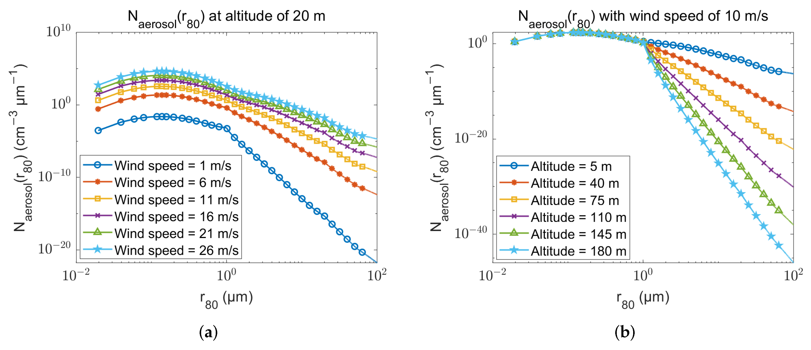
2.1.1. SSA Size Distribution Model

On sunny days, atmospheric aerosol is the primary propagation and scattering medium of electromagnetic waves. Atmospheric aerosol comes from a variety of sources, including natural mechanisms of the Earth’s surface, anthropogenic gas emissions, and volcanic eruptions. Therefore, there are considerable variations in aerosol components across different regions, seasons, and altitudes [20,21]. In undisturbed marine environments far from continental and anthropogenic sources, SSA particles are often the dominant component. Predominantly formed by the action of the sea surface wind, SSA mainly exists below 0.5 km and comprises seawater droplets and dry sea salt particles. As the radii of SSA particles always change with different humidity levels, to avoid confusion, the size of SSA particles is often described with the equilibrium radius at the standard relative humidity 80%, denoted as $r_{80}$ [22,23]. The equivalent dry radius $r_{\mathrm{d}}$ is another parameter that characterizes the size of SSA. Because $r_{\mathrm{d}}$ describes the bulk of dry sea salt and is not related to humidity, it is always used to convert the measurements to the corresponding value at a certain relative humidity level. The equilibrium droplet radius $r_{\mathrm{eq}}$ at a given relative humidity $RH$ (in decimal form) can be converted from $r_{\mathrm{d}}$ with the following equations [24,25]:

$$r_{\mathrm{eq}}=\alpha \left(RH\right)r_{\mathrm{d}}^{\beta \left(RH\right)}$$

(1)

$$\alpha \left(RH\right)=1.62exp\left(\frac{0.066RH}{g\left(RH\right)-RH}\right)$$

(2)

$$g\left(RH\right)=\left\{\begin{array}{c}1.058,RH<0.97\hfill \\ 1.058-{\displaystyle \frac{0.0155(RH-0.97)}{1.02-R{H}^{1.4}}},0.97<RH<0.995\hfill \end{array}\right.$$

(3)

$$\beta \left(RH\right)=exp\left(\frac{0.00077RH}{1.009-RH}\right),0.80<RH<0.995$$

(4)

Numerous investigations on the size distribution models of SSA were conducted as a result of the significant impact of SSA on various remote sensing and environmental monitoring applications [26,27,28,29]. Among these models, the Advanced Navy Aerosol Model (ANAM) [29], which was derived from the Navy Aerosol Model [30], has been widely used after years of data validation since 1983.

According to the ANAM, the sea spray source function (S3F) needs to be calculated first, which reflects the rate of seawater droplet generation per unit area of the ocean surface [23]. Two types of S3Fs have been selected for the ANAM, i.e., the S3F_SH (see (5) and (6)) derived by Smith and Harrison, which is mainly for large particles [31], and the S3F_V (see (7)) derived by Vignati et al., which is mainly for small particles [32]:

$$\frac{\mathrm{d}F}{\mathrm{d}{r}_{80}}=\sum _{i=1}^2{A}_{i}exp\left\{-f_{\mathrm{i}}{\left[ln(r_{80}/r_{0i})\right]}^2\right\},$$

(5)

$$\left\{\begin{array}{c}{A}_1=0.2U_{10}^{3.5}\hfill \\ A_2=0.0068U_{10}^3\hfill \end{array}\right.,$$

(6)

$$\frac{\mathrm{d}F}{\mathrm{d}{log}_{10}{r}_{80}}=\sum _{i=1}^3\frac{N_i}{\sqrt{2\pi }{log}_{10}{\sigma }_i}exp\left[-\frac{{({log}_{10}{r}_{80}-{log}_{10}{R}_i)}^2}{2{log}_{10}^2{\sigma }_i}\right],$$

(7)

where $r_{01}=3$ $\mathsf{\mu }$m, $r_{02}=30$ $\mathsf{\mu }$m, $f_1=1.5$, $f_2=1$, and $U_{10}$ (m/s) is the wind speed at an altitude of 10 m. $N_i$, $R_i$, and ${\sigma }_i$ in (7) can be found in Table 1 of reference [29].

In the calculation process, S3F_SH and S3F_V are merged into a piecewise function, where the transition occurs at a dry radius of 4 $\mathsf{\mu }$m. The relationship between $r_{80}$ and $r_{\mathrm{d}}$ is shown in (1). When the two S3Fs do not match at the switch point due to the difference in intensity and wind speed dependence, the practical solution is to multiply S3F_V by a radius-independent constant to match S3F_SH, given that the larger particles in S3F_SH have relatively short residence times and their concentration varies more significantly with different wind speeds.

Based on the combined S3F, the aerosol particle size distribution above the sea surface, i.e., $N_{\mathrm{aerosol}}(r_{80},z=0)$, is described in (8) and (9). Then, the aerosol particle size distribution at a certain altitude z can be calculated with $f_{\mathrm{ab}}\left(z\right)$, which governs the decrease in $N_{\mathrm{aerosol}}\left(r_{80}\right)$ as a function of the altitude, as shown in (10)–(12). In these equations, $P_1$, $P_2$, $P_3$, and $P_4$ are all empirical tuning parameters and their values depend on the datasets from different sea areas. In this study, the empirical parameters were set to $P_1=2.5,P_2=0.3,P_3=3.0$, and $P_4=0.8$, which are the optimal values for an open ocean dataset, as shown in Table 2 of reference [29].

$$N_{\mathrm{aerosol}}(r_{80},z=0)={10}^{P_{1}Y}\frac{\mathrm{d}F}{\mathrm{d}{r}_{80}}$$

(8)

$$\left\{\begin{array}{c}X=1.0-{\displaystyle \frac{{log}_{10}\left(20.0\right)}{{log}_{10}\left(r_{80}\right)}}\hfill \\ Y=max(0.25,1.0-X\times P_3)\hfill \end{array}\right.$$

(9)

$$N_{\mathrm{aerosol}}(r_{80},z)=f_{\mathrm{ab}}\left(z\right)\times N_{\mathrm{aerosol}}(r_{80},z=0)$$

(10)

$$f_{\mathrm{ab}}\left(z\right)=exp(-1.0\times P_2\times f_{\mathrm{a}}\left(r\right)\times f_{\mathrm{b}}\left(U\right)\times z)$$

(11)

$$\left\{\begin{array}{cc}{f}_{\mathrm{a}}\left(r\right)={log}_{10}^{P_4}\left(r_{80}\right)\hfill & r_{80}>1\hfill \\ f_{\mathrm{b}}\left(U\right)=3.0-(2\times {log}_{10}\left(U_{10}\right))\hfill & U_{10}>1\hfill \end{array}\right.$$

(12)

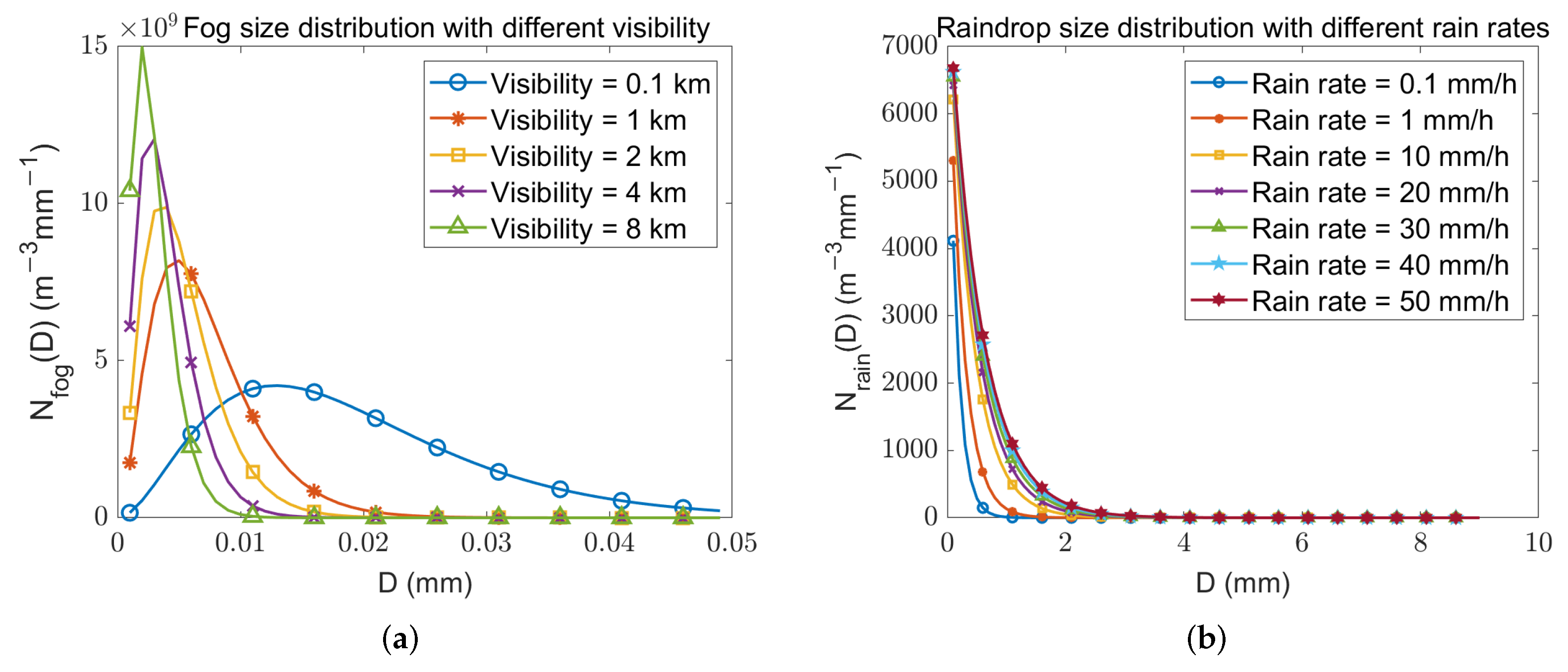
2.1.2. Fog Droplet Size Distribution Model

Fog is one of the most dangerous weather conditions above the sea surface due to its significant impact on visibility [33]. Fog is typically classified into two types based on its location and formation mechanism: advection fog (predominantly at sea) and radiation fog (primarily on land) [34]. The radius of fog droplets generally ranges from 2 $\mathsf{\mu }$m to 15 $\mathsf{\mu }$m, with a maximum radius of 50 $\mathsf{\mu }$m [26]. Equation (13) gives the fog particle size distribution model for advection fog [35]:

$$N_{\mathrm{fog}}\left(r\right)=1.059\times {10}^7\times V^{1.15}{r}^2{\mathrm{e}}^{-0.8359V^{0.43}r},$$

(13)

where $N_{\mathrm{fog}}\left(r\right)\left({\mathrm{m}}^{-3}\mathsf{\mu }{\mathrm{m}}^{-1}\right)$ is the number of fog droplets within the interval of unit volume and unit diameter, r ($\mathsf{\mu }$m) denotes the radius of fog droplet, and V (km) is the visibility.

2.1.3. Raindrop Size Distribution Model

Rain is another common meteorological condition that significantly impacts the detection range of remote sensing instruments. Raindrops in nature are often nonspherical due to air resistance compression. The meteorological community generally takes the oblate shape as a good approximation of a raindrop’s shape, and the equivolumetric spherical drop diameter D (mm) (hereinafter, diameter) is typically used to characterize the drop size [36], which usually ranges from 0.1 mm to 9 mm. Among the raindrop size distribution models [30,37,38], the normalized gamma distribution model has the best adaptability to different rainfall types in nature [39], and the exponential model proposed by Marshall et al. [40] presents similar results to the normalized gamma distribution model in our experiments. Given that the exponential model takes the rain rate as the sole independent variable, which is beneficial for directly illustrating the relationship between the rain rate and instrument performance, it was applied in the subsequent experiments, as shown in (14):

$$N_{\mathrm{rain}}\left(D\right)=8000exp(-4.1{\gamma }^{-0.21}D),$$

(14)

where $N_{\mathrm{rain}}\left(D\right)\left({\mathrm{m}}^{-3}{\mathrm{mm}}^{-1}\right)$ is the number of raindrops within the interval of the unit volume and unit diameter, and $\gamma$ (mm/h) is the rain rate.

2.2. Electromagnetic Properties of Particles

The electromagnetic properties of particles serve as a link between remote sensing measurements and the physical properties of particles, and the appropriate modeling of electromagnetic properties is helpful to reveal the influence of transmission media on the instrument performance. Up to now, several approaches for electromagnetic properties simulation have been established, including Mie theory and its extensions, as well as the T-matrix method [41], and each of them is suitable for specific particle shapes and electric sizes [42] ($\chi =2\pi r/\lambda$, representing the ratio of the particle radius r to the wavelength $\lambda$).

The T-matrix method is introduced here as one of the most well-known methods to simulate electromagnetic properties of nonspherical particles, as raindrops are typically oblate rather than spherical [43]. The PyTMatrix package, which was designed by Leinonen with Python code, provides a simple and extensible interface for the T-matrix method [44,45]. With the PyTMatrix package, the backscattering cross-section ${\sigma }_{bcca}$ and extinction cross-section ${\sigma }_{\mathrm{ext}}$ can be obtained by inputting the physical properties of particles.

However, the T-matrix method is only suitable for electric sizes less than 100; otherwise, the calculation process is more likely to be ill-conditioned [17,45]. To avoid this problem, the Mie theory [46] is introduced as a supplement for large electric size cases, such as the fog droplets or raindrops under the scanning of lidar where the electric size may reach hundreds or even thousands. The backscattering cross-section ${\sigma }_{\mathrm{bsca}}$ and extinction cross-section ${\sigma }_{\mathrm{ext}}$ can be computed based on Mie theory with the equations below:

$${\sigma }_{\mathrm{bsca}}=\underset{r_{\min }}{\overset{r_{\max }}{\int }}\pi r^2{Q}_{\mathrm{bac}}\left(r\right)N\left(r\right)dr,$$

(15)

$${\sigma }_{\mathrm{ext}}=\underset{r_{\min }}{\overset{r_{\max }}{\int }}\pi r^2{Q}_{\mathrm{ext}}\left(r\right)N\left(r\right)dr,$$

(16)

$$Q_{\mathrm{bac}}\left(r\right)=\frac{1}{\chi {\left(r\right)}^2}{\left|\sum _{n=1}^{\infty }(2n+1){(-1)}^n(a_n-b_n)\right|}^2,$$

(17)

$$Q_{\mathrm{ext}}\left(r\right)=\frac{2}{\chi {\left(r\right)}^2}\sum _{n=1}^{\infty }(2n+1)\mathrm{Re}(a_n+b_n),$$

(18)

where $r_{\min }$ and $r_{\max }$ are the minimum and maximum radii of scattering particles; $N\left(r\right)$ is the number of particles with radius r in a unit volume; and $Q_{\mathrm{bac}}\left(r\right)$ and $Q_{\mathrm{ext}}\left(r\right)$ are the backscattering coefficient and extinction coefficient of a single particle with radius r, and they are determined by the size parameter $\chi$ and Mie coefficients $a_n$ and $b_n$. The calculation of $a_n$ and $b_n$ involves iterative calculations, and details can be found in reference [46].

2.3. Detection Principles of Radar and Lidar

In essence, the detection principles of radar and lidar are similar. They both transmit electromagnetic waves and then receive and analyze the echo from the targets to obtain the physical characteristics of the scattering medium. The radar and lidar equations in (19) and (20) illustrate the basic principles of radar/lidar detection [18]:

$$P_{\mathrm{r}}=P_{\mathrm{t}}\frac{G^2{\lambda }^2\Delta \varphi \Delta \theta \tau c}{2^{10}{\pi }^2{R}^{2}ln2}{\sigma }_{\mathrm{bsca}}\times {10}^{-0.2{\int }_0^R{\sigma }_{\mathrm{ext}}dl},$$

(19)

$$P_{\mathrm{l}}=P_{\mathrm{t}}\frac{\tau cA}{R^2}{\sigma }_{\mathrm{bsca}}\times e^{-2{\int }_0^R{\sigma }_{\mathrm{ext}}dl},$$

(20)

where $P_{\mathrm{t}}$ is the transmitting power, $P_{\mathrm{r}}$ / $P_{\mathrm{l}}$ is the echo power of the radar/lidar; G is the radar antenna gain; $\lambda$ is the radar wavelength; $\Delta \varphi$ and $\Delta \theta$ are the beam width along the elevation and azimuthal directions, respectively; $\tau$ is the pulse time; $c=3\times {10}^8$ m/s is the speed of light; R is the detection range; ${\sigma }_{\mathrm{bsca}}$ and ${\sigma }_{\mathrm{ext}}$ are the backscattering cross-section and extinction cross-section of the target, respectively; and A is the area of the aperture of the receiving antenna.

Generally, the maximum detection range $R_{\max }$ for radar/lidar is defined as the range where the echo power is equal to the receiver sensitivity $S_{\min }$. $S_{\min }$ is determined by the minimum detectable signal-to-noise ratio (SNR) ${(S/N)}_{\min }$ and the receiver noise $P_{\mathrm{n}}$. This relationship is as follows:

$$S_{min}=P_{\mathrm{n}}{(S/N)}_{\min },$$

(21)

$$P_{{\mathrm{n}}_{-}\mathrm{r}}=K{T}_0{B}_{\mathrm{n}}{F}_{\mathrm{n}},$$

(22)

$$P_{\mathrm{n}\_\mathrm{l}}=2\frac{e_c^2\eta B_{\mathrm{n}}}{\mathrm{hf}}{P}_{\mathrm{L}},$$

(23)

where $P_{{\mathrm{n}}_{-}\mathrm{r}}$ and $P_{\mathrm{n}\_\mathrm{l}}$ are the receiver noises for the radar and lidar systems, respectively; $K=1.38\times {10}^{-23}$ J/K is the Boltzmann constant; $T_0$ is the absolute temperature and is typically set to 290 K; $B_{\mathrm{n}}$ is the noise bandwidth; $F_{\mathrm{n}}$ is the noise figure; $e_c$ is the electron charge; $\eta$ is the quantum efficiency; h is Plank’s constant; f is the frequency; and $P_{\mathrm{L}}$ is the power of the reference beam [47].

In practice, data accumulation is always adopted to indirectly increase $R_{\max }$. In general, the coherent accumulation of $n_{\mathrm{p}}$ measurements can improve ${(S/N)}_{\min }$ by $n_{\mathrm{p}}$ times, while the noncoherent accumulation gain is approximately $n_{\mathrm{p}}^{\varrho }$, with $\varrho$ ranging from 0.8 (for small $n_{\mathrm{p}}$) to 0.5 (for large $n_{\mathrm{p}}$) [48]. That is to say, $S_{\min }$ can be improved by $n_{\mathrm{p}}$ /$n_{\mathrm{p}}^{\varrho }$ times with the coherent/noncoherent accumulation of $n_{\mathrm{p}}$ measurements.

Except for $S_{\min }$, another parameter that needs to be considered is the velocity variance ${\sigma }_{\mathrm{v}}^2$. It characterizes the accuracy of velocity detection and is also relative to the SNR, as shown in (24)–(26):

$${\sigma }_{\mathrm{v}\_\mathrm{r}}^2=\frac{{\lambda }^2}{4M{T}_{\mathrm{s}}}\left[\frac{{\delta }_{\mathrm{vn}}}{4\sqrt{\pi }}+2{\left({\delta }_{\mathrm{vn}}\right)}^2/\mathrm{SNR}+\frac{1}{12{\mathrm{SNR}}^2}\right],$$

(24)

$${\delta }_{\mathrm{vn}}=\frac{2{\delta }_{\mathrm{v}}{T}_{\mathrm{s}}}{\lambda },$$

(25)

$${\sigma }_{\mathrm{v}\_\mathrm{l}}^2={\left(\frac{\lambda }{2}\frac{\sqrt{3}}{\pi \tau \sqrt{2\mathrm{SNR}}}\right)}^2,$$

(26)

where ${\sigma }_{\mathrm{v}\_\mathrm{r}}^2$ and ${\sigma }_{\mathrm{v}\_\mathrm{l}}^2$ are the velocity variances for radar and lidar detection, respectively; M is the number of signal samples processed; $T_{\mathrm{s}}$ is the pulse repetition period; and ${\delta }_{\mathrm{v}}$ is the width of Doppler spectrum [49].

According to the equations above, the accuracy of the velocity is positively correlated with the SNR. When the SNR is lower than a certain threshold, the interpreted speed information is not reliable, even if the signal can be received successfully. Therefore, both ${\sigma }_{\mathrm{v}}^2$ and $S_{\min }$ should be considered to determine the minimum value of the echo power when evaluating the performance of radar/lidar.

2.4. Key Parameters

Currently, given the complexity of oceanic environments and the need for aviation support, shipborne wind lidars generally have a wavelength of 1.55 $\mathsf{\mu }$m [50], and other typical parameters are as follows: $P_{\mathrm{t}}=100$ $\mathsf{\mu }$J, $\tau =400$ ns, $S_{min}=-90$ dBm, and an antenna diameter of 10 cm. Meanwhile, for radars, the typical bands used for meteorological observation include S-, C-, X-, Ka-, and W-bands, and these bands were all considered in our simulation to find an optimal combination scheme. The key parameters of these radars refer to several classic papers [51,52], as shown in

Table 1. Key parameters of radars.

Band	Frequency (GHz)	Transmission Power (kW)	Antenna Gain (dB)	Beam Width ($°$)	Pulse Time (μs)	Receiver Sensitivity (dBm)
S	2.89	650.0	44	0.95	1.57	−109
C	5.43	250.0	44	1.00	1.00	−107
X	9.38	30.0	44	1.00	1.00	−114
Ka	34.88	3.0	53	0.40	1.50	−106
W	93.75	1.5	59	0.16	0.50	−104

. To improve the credibility of this simulation, noncoherent and coherent accumulation were adopted for lidar and radars, respectively, and the number of accumulated pulses followed a time resolution of 0.5 s.

Notably, the complex refractive index m plays an important role in the computation of electromagnetic characteristics, and it is determined by both the component of the substance and the frequency of the incident wave. The primary component of rain and fog is water, and thus, their complex refractive index is equivalent to that of water, which can be easily obtained at https://refractiveindex.info/ (accessed on 20 September 2023). However, no such systematic investigation of SSA has been conducted yet. Frederic investigated the complex refractive index of dry natural substances and sea salt with wavelengths ranging from 2.5 to 40 $\mathsf{\mu }$m [53], and Li et al. set the complex refractive index of aerosol to 1.53 + 0.03i in their study of optical scattering communication under various aerosol types (including maritime aerosol) [21], which approximately conforms to the study of Frederic. Thus, in this work, the complex refractive index of aerosol for lidar scanning was also set to 1.53 + 0.03i. In the microwave bands, the complex refractive index of SSA was set the same as that of seawater since SSA is primarily produced by burst bubbles and broken ocean wave crests [22]. The Debye equation describes the complex relative permittivity of seawater at various frequencies within the microwave band, and Klein et al. expressed the parameters of the Debye equation as functions of temperature, salinity, and frequency [54]. On this basis, the complex refractive index of SSA within the microwave band could be obtained with $m=\sqrt{\epsilon }$, setting the temperature and salinity as common values of 25 and 35. All the complex refractive indices used in this work are summarized in

Table 2. Complex refractive indices.

Band	Wavelength (mm)	m for Rain/Fog	m for SSA
S	103.98	8.75 + 0.62i	8.69 + 2.43i
C	55.24	8.55 + 1.11i	8.40 + 2.04i
X	31.98	8.15 + 1.74i	7.99 + 2.23i
Ka	8.60	5.49 + 2.83i	5.53 + 2.89i
W	3.20	3.47 + 2.14i	3.60 + 2.01i
Near-infrared	1.55 $\times {10}^{-3}$	1.31 + 2.24 $\times {10}^{-4}$i	1.53 + 0.03i

.

3. Results

3.1. Electromagnetic Characteristics Analysis

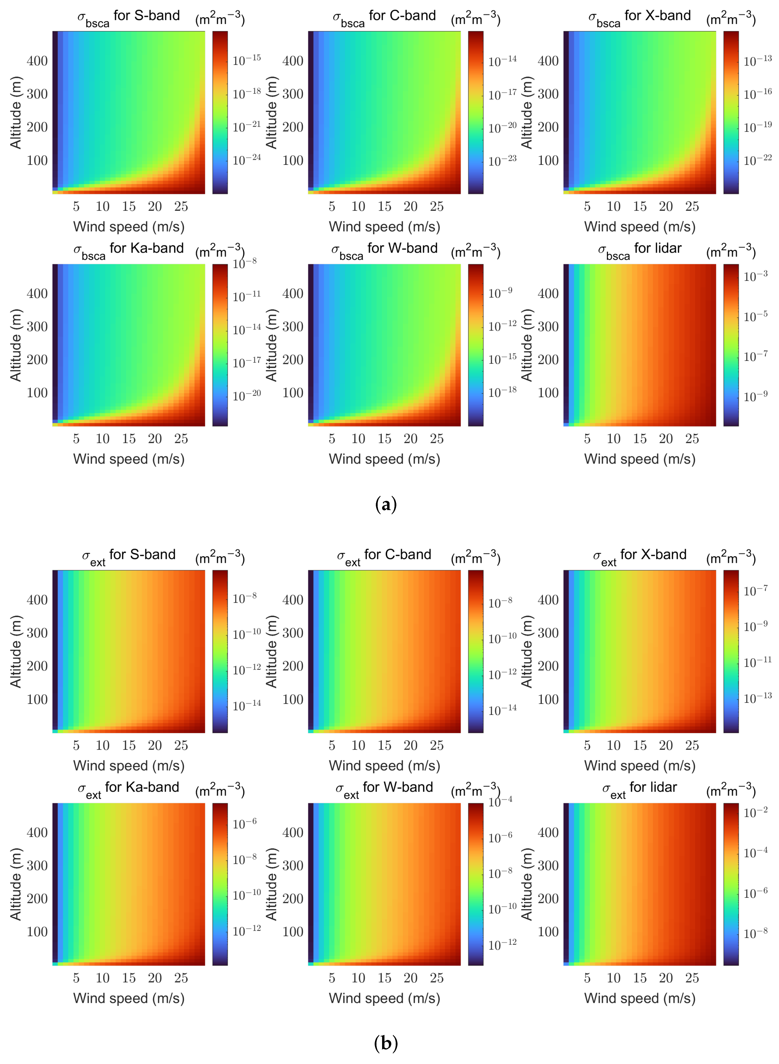
3.1.1. Scattering and Attenuation in Sea Salt Aerosol

As suggested above, the SSA particle size distribution model $N_{\mathrm{aerosol}}\left(r_{80}\right)$ on sunny days was based on the ANAM and the range of $r_{80}$ in simulations was set from 0.01 to 100 $\mathsf{\mu }$m [28,29,55]. According to Section 2, $N_{\mathrm{aerosol}}\left(r_{80}\right)$ was mainly determined by the sea surface wind and the altitude from the sea surface. The influence of the two parameters on $N_{\mathrm{aerosol}}\left(r_{80}\right)$ is depicted in Figure 1. Obviously, particles of all sizes fluctuated with changes in wind speed, but only particles larger than 1 $\mathsf{\mu }$m were sensitive to a change in altitude. What is more, larger particles showed a higher sensitivity to changes in altitude. The threshold of 1 $\mathsf{\mu }$m may not fully represent reality, but it should provide a reasonable approximation for the simulation of the aerosol particle size distribution given the extensive data analysis of the ANAM. Additionally, both Lewis et al. and Kaloshin et al. also mentioned that the influence of gravity and the vertical concentration gradient on SSA particles smaller than 1 $\mathsf{\mu }$m were negligible [23,28].

Figure 2 shows the variations in ${\sigma }_{\mathrm{bsca}}$ and ${\sigma }_{\mathrm{ext}}$ with different wind speeds and altitudes. From Figure 2, two conclusions could be drawn:

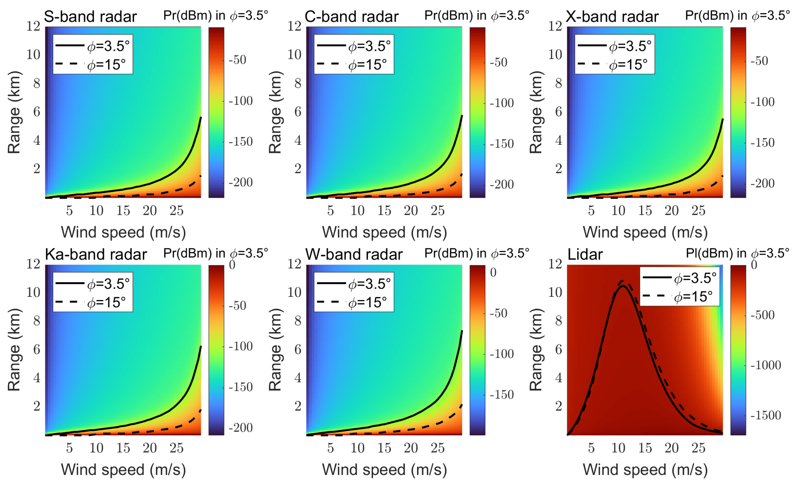
• The wind speed had a positive correlation with ${\sigma }_{\mathrm{bsca}}$/${\sigma }_{\mathrm{ext}}$, while the altitude negatively correlated with them, which was entirely consistent with the changes in $N_{aerosol}\left(r_{80}\right)$. Furthermore, with increasing altitude, the ${\sigma }_{\mathrm{bsca}}$ of the radar decreased more rapidly than that of the lidar, indicating that the performance of the radar decreased faster with the altitude increase.
• Within the same range of wind speed and altitude, the ${\sigma }_{\mathrm{bsca}}$ and ${\sigma }_{\mathrm{ext}}$ of the lidar were at the same level, while the ${\sigma }_{\mathrm{ext}}$ of the radar was several orders of magnitude greater than its ${\sigma }_{\mathrm{bsca}}$, which implies that the detection range of lidar should outperform that of radar.

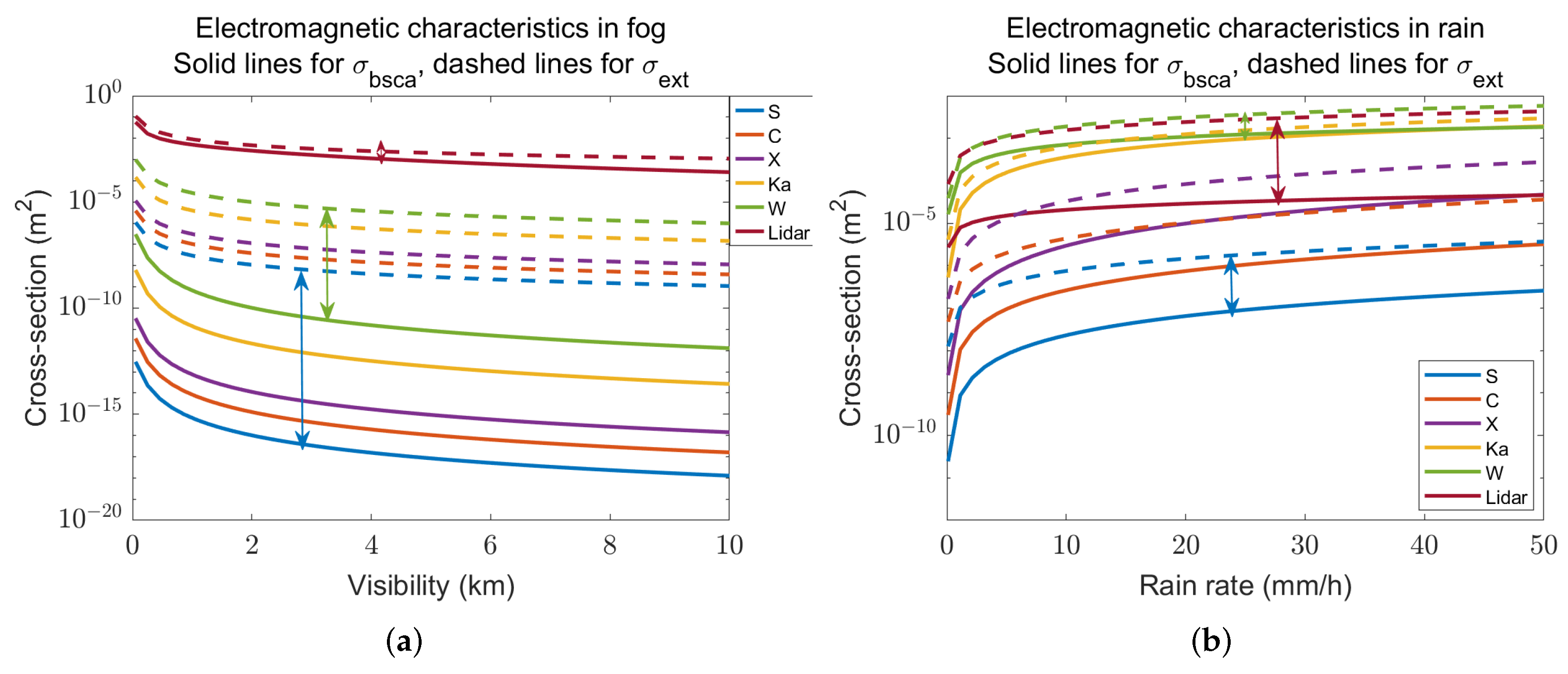
3.1.2. Scattering and Attenuation in Fog and Rain

According to the classification by the China Meteorological Administration, a fog warning typically indicates visibility of less than 1 km. In detail, the visibility threshold for strong fog, thick fog, heavy fog, fog, and mist are 50 m, 200 m, 500 m, 1 km, and 10 km, respectively. Thereby, in this study, the visibility value in fog was set from 50 m to 10 km. As for rainfall cases, the rain rate is always in the range from 0.1 mm/h to 12 mm/h, including light rain and heavy rainstorms. Furthermore, in the field experiment of Oude Nijhuis et al., the rain rate was once up to 50 mm/h [12]. Although extreme rainfall cases are relatively rare, they were considered here for the sake of completeness. Thus, the rain rate in this simulation was set to range from 0.1 mm/h to 50 mm/h.

Based on the models in Section 2, the relationship between $N_{\mathrm{fog}}\left(D\right)$/$N_{\mathrm{rain}}\left(D\right)$ and visibility/rain rate was simulated, as shown in Figure 3. By comparing the two subgraphs, it can be seen that the size of the fog droplets was mainly concentrated within 0.02 mm, two orders of magnitude smaller than the main size of raindrops. The other way around, the concentration of fog droplets was much higher than that of raindrops. The two differences determined the distinct electromagnetic characteristics of fog and rain, as shown in Figure 4.

In Figure 4, the solid and dashed lines represent ${\sigma }_{\mathrm{bsca}}$ and ${\sigma }_{\mathrm{ext}}$, respectively, with different colors indicating different wave bands. The blue, green, and red double-headed arrows illustrate the differences between ${\sigma }_{\mathrm{ext}}$ and ${\sigma }_{\mathrm{bsca}}$ of the S-band radar (the lowest frequency in radars), W-band radar (the highest frequency in radars), and lidar, respectively.

Analysis of Figure 4 allowed for three deductions:

• In the first subgraph, the ${\sigma }_{\mathrm{bsca}}$ values of the radars were significantly smaller than that of the lidar, which suggests that the performance of the radars in fog may have been limited by their weak sensing ability to fog droplets, especially in cases of high visibility.
• In the second subgraph, the ${\sigma }_{\mathrm{bsca}}$ of the lidar lay between that of the low-frequency (S/C/X) and high-frequency (Ka/W) microwave radars, and the difference between the ${\sigma }_{\mathrm{ext}}$ and ${\sigma }_{\mathrm{bsca}}$ of the lidar was the largest among those simulated cases, as indicated by the double-headed arrows. This implies that the attenuation effect of the lidar in the rain should be more pronounced than that of the radars.
• Compared with the fog cases, the ${\sigma }_{\mathrm{bsca}}$ values of the radars in the rain cases exhibited a significant increase, while the ${\sigma }_{\mathrm{ext}}$ values of radars remained relatively stable. Thus, the detection performance of radars in the rain should surpass that in fog.

3.2. Calculation of the Maximum Detection Range

3.2.1. The Maximum Detection Range on Sunny Days

With ${\sigma }_{\mathrm{bsca}}$ and ${\sigma }_{\mathrm{ext}}$ of SSA, the echo power was calculated across a range of elevation angles $\varphi$ and wind speeds based on instrument parameters concluded in Table 1. Elevation angles were considered here because the altitude, relative to $N_{\mathrm{aerosol}}\left(r_{80}\right)$, varied with detection ranges and elevation angles. Figure 5 illustrates the impact of elevation angles and wind speeds on the performances of the lidar and radars. $R_{\max }$ indicates the critical point where the echo power was equal to the receiver sensitivity and the velocity variance of the Doppler system met the requirements, as drawn with black curves, where the solid and dashed curves are for $\varphi ={3.5}^{\circ }$ and $\varphi ={15}^{\circ }$, respectively.

According to the results shown in Figure 5, the following conclusions could be drawn for sunny days:

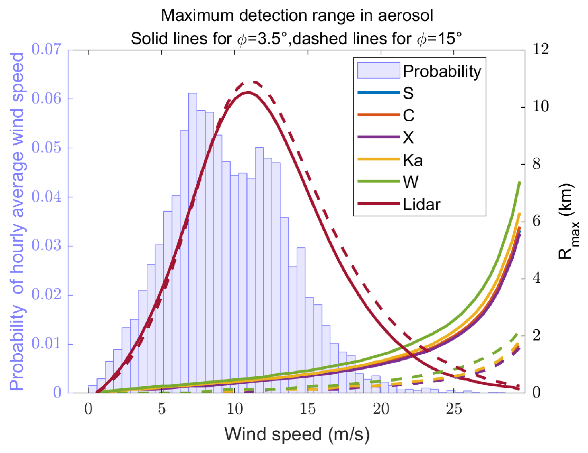
• The radars with different bands could only detect wind at high wind speeds because the radars were only sensitive to large SSA particles that appeared under these conditions. Furthermore, because of the vertical concentration gradient of large SSA particles, the radar performance at a low elevation angle was better than that at a high elevation angle.
• Compared with the radars, the lidar was more suitable for medium wind speed conditions because the high concentration of aerosols under high wind speed conditions led to a sharp attenuation of the laser.
• The radars could partially fill the gap of lidar detection at high wind speeds, especially under low elevation angles.

3.2.2. The Maximum Detection Range in Precipitation

By combining the instrument parameters and the electromagnetic characteristics of scattering media under varying intensities of fog and rainfall conditions, the echo power and corresponding $R_{\max }$ of the radars and lidar were calculated, as depicted in Figure 6 and Figure 7.

Figure 6 shows the instrument performance in fog with different visibility, where the pseudocolor maps and dashed lines mean the echo power and the maximum detection range of each instrument, respectively. The smaller the visibility, the greater the fog intensity. From the curve distribution of each subgraph, the following could be concluded:

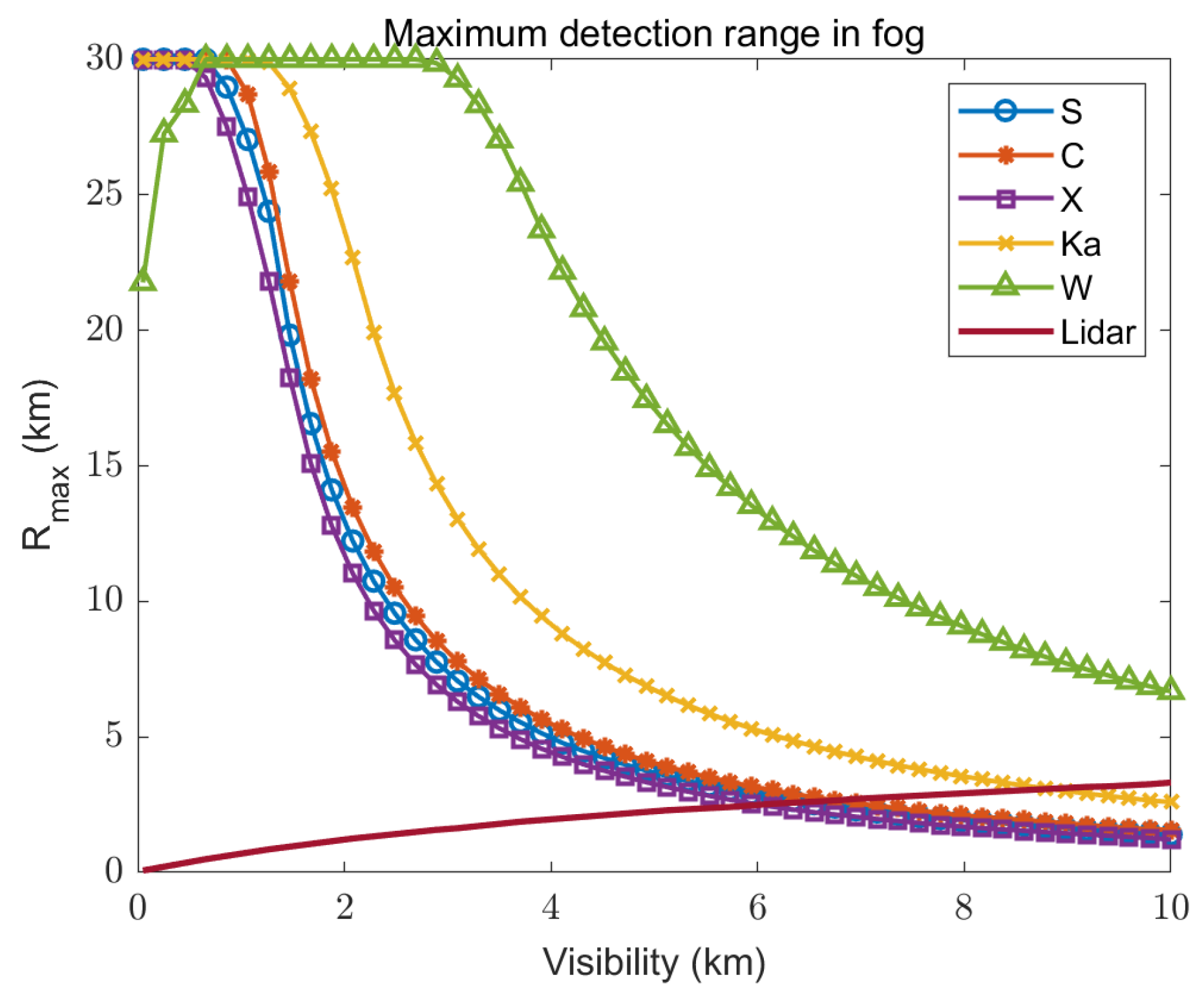
• Compared with the misty weather, the radars were more suitable for detection in the dense fog weather. At this time, there were enough fog droplets in the space to provide backscatter signals for the radars.
• It should be noted that for the high-frequency radars, such as the W-band radars, thicker fog also meant more obvious signal attenuation, and thus, too small of a visibility could lead to a decrease in the maximum detection range.
• The attenuation effect of the laser in fog was significant. Even under high visibility conditions, the maximum detection range of the lidar did not exceed 5 km.

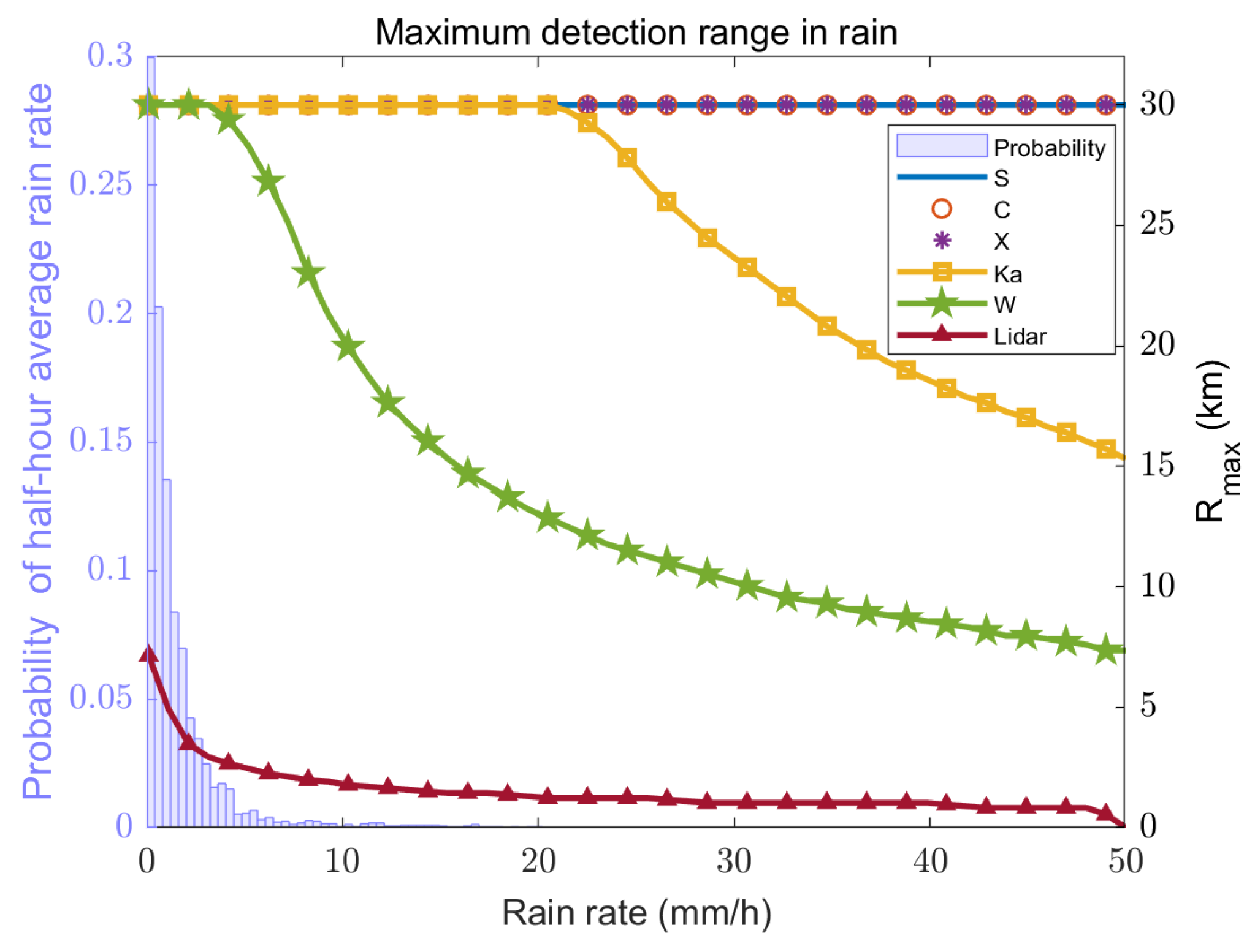
These results align with the field experiments of Oude Nijhuis and Ritvanen, which showed that X-band radar and lidar are insufficient for detection in fog, and external sources of information are required [12,14]. According to our results, the sensitivity of the W-band radar to fog droplets was higher than that of the X-band radar.

Figure 7 presents the simulation results in the rain cases. In fact, $R_{\max }$ of the S/C/X-band radars exceeded 30 km, but 30 km was set as an upper limit here because a detection distance of 30 km already satisfies most requirements. Obviously, for the S-, C-, and X-band radars, signal attenuation in the rain was too minor to impact the detectable range. For the Ka- and W-band radars, $R_{\max }$ decreased by up to 50% and 75%, respectively, when the rain rate increased to 50 mm/h, but their detectable ranges were more than 5 km, even under heavy rain conditions. In comparison, the lidar performed much worse, with the $R_{\max }$ limited to only about 1–2 km. For rain cases, we could conclude the following:

• The $R_{\max }$ of the S-, C-, and X-band radars exceeded that of the Ka- and W-band radars in heavy rain, but the Ka- and W-band radars could also meet the needs of short-range wind field detection (at least 5 km), despite the obvious signal attenuation.
• All the microwave radars performed better than the lidar due to the sharp attenuation of laser beams in the rain, and joint detection was almost unnecessary when only considering the maximum detection distance.

4. Discussion

4.1. Instrument Performance Analysis

According to the simulation results, Section 3 presents the maximum detection range of each instrument on sunny, foggy, and rainy days. To better demonstrate the detection capabilities of these instruments, this part further analyzes the instrument performance with measured weather data from an all-weather perspective.

The curves in Figure 5 display the $R_{\max }$ of the radars and lidar across various elevation angles and wind speeds, with different colors representing different instruments and the solid/dashed curves indicating $\varphi ={3.5}^{\circ }$/$\varphi ={15}^{\circ }$. For a more straightforward comparison, Figure 8 plots these curves together and adds a histogram of the statistical probability distribution of the hourly average wind speed in 2022. The statistical data, which was obtained from the Copernicus Climate Change Service (C3S) Climate Data Store [56], corresponded to the location at $27.5^{\circ }$ east longitude and $123.5^{\circ }$ north latitude, and the pressure level at 975 hPa (about 300 m above sea level). According to the annual statistics data, the wind speeds were mainly concentrated in the moderate range, i.e., from 5 to 15 m/s, which corresponded to the range where lidar has strong detection capabilities. Therefore, for a single-instrument system, lidar is more suitable for wind field detection under clear sky conditions than radars. For a dual-instrument system, the combination of lidar and W-band radar should perform better than other combinations and can cover most of the wind speed scenarios, except for minimal wind speed cases where the effect of wind on activities is negligible.

Similar to Figure 8, Figure 9 and Figure 10, we compared the curves of $R_{\max }$ of each instrument in the fog and rain. Unfortunately, we did not find any statistical data on sea fog visibility, and thus, there is no histogram included in Figure 9. By comparing the curves in Figure 9, it is evident that the W-band radar had the best adaptability to different visibility conditions in fog. Additionally, the maximum detection range of the lidar was consistently shorter than that of the W-band radar. As for rainy days, the annual half-hour average rain rate statistical histogram is included in Figure 10 for a more intuitive demonstration of instruments’ performance, which came from the Goddard Earth Sciences Data and Information Services Center [57] and corresponded to the location at $27.5^{\circ }$ east longitude and $123.5^{\circ }$ north latitude in 2022. From the annual statistical data, we can see that the rain rate predominantly fell within 10 mm/h. Even when the requisite detection distance was set to a minimum of 10 km, each radar band, including the W-band radar, which exhibited a pronounced attenuation effect, was still capable of covering 99% of the rainfall cases. Therefore, the detection performances of the radars were always superior to that of the lidar, and their complementary characteristics were not significant in precipitation.

4.2. Combination Strategy

According to the analysis above, due to the influence of the electromagnetic scattering characteristics of different propagation media, lidar and microwave radars are suitable for clear sky conditions and precipitation conditions, respectively. It is difficult for a single lidar or microwave radar to detect marine wind under all-weather conditions. Furthermore, the complementarity of lidar and radars also exists on sunny days under different wind speed conditions. Therefore, a combination strategy involving lidar and microwave radar is necessary. Comparing the maximum detection range of microwave radars in different bands, the W-band radar performed best on both sunny and foggy days but performed worst in heavy rain due to the serious attenuation effect. However, considering the small probability of a rainfall rate greater than 15 mm/h, we still recommend the combination of lidar and W-band radar for sea surface wind detection under all-weather conditions. This is a compromise tailored to our case location (27.5°E, 123.5°N), sacrificing system detection performance under heavy rain conditions to ensure broader adaptability in clear and foggy weather.

The above analysis is based on the typical equipment parameters we surveyed. In real applications, it may be necessary to analyze more specific equipment parameters and environmental parameters. Considering this need, we provide the simulated dataset of ${\sigma }_{\mathrm{bsca}}$ and ${\sigma }_{\mathrm{ext}}$ with different radar bands and environmental conditions, which can be found in https://github.com/limilyli/Radar-parameter-design/tree/master (accessed on 29 April 2024), and subsequent research on the detection system can be carried out on this dataset. To provide a better theoretical basis for the design of the detection system, a software package was designed and released on the same website to calculate the fundamental prerequisites that the detection system should meet to satisfy a specified detection requirement. In detail, the radar equation was adjusted so that the key radar parameters (left part in (27)) were separated from the detection parameters and environmental parameters (right part in (27)). The detection parameters included the maximum detection range, elevation angle, and radar band, and the environmental parameters included wind speed/visibility/rain rate on sunny/foggy/rainy days. Once the detection parameters and environmental parameters were determined, the lower limit of those key radar parameters could be obtained with the software package, and a summary of the process of the software is shown in Figure 11.

$$\frac{P_{\mathrm{t}}{G}^2\Delta \varphi \Delta \theta \tau }{S_{min}}>max\left(\frac{2^{10}{\pi }^2{R}^{2}ln2}{{\lambda }^{2}c{\sigma }_{\mathrm{bsca}}\times {10}^{-0.2\underset{0}{\overset{R}{\int }}{\sigma }_{\mathrm{ext}}dl}}\right)$$

(27)

4.3. Potential Improvements

Due to the lack of sufficient measured data, this study primarily relied on theoretical and simulation experiments to analyze the complementary characteristics of lidar and microwave radars in detecting sea surface wind fields under all-weather conditions. In the next phase, we plan to conduct sea surface detection experiments, focusing on the remote sensing of fine-scale sea surface wind fields. By incorporating experimental data, we aim to further validate and extend the conclusions of this study.

Additionally, this study only considered the three most common weather conditions: sunny, foggy, and rainy days. In the future, we plan to include research on extreme weather conditions, such as snow and hail, to further broaden the all-weather applicability of our findings.

5. Conclusions

Accurate marine wind detection is a prerequisite for both military and civilian activities. Microwave radars and lidar are two types of instruments that balance high spatiotemporal resolution and large-scale detection. However, the detection capability boundaries of these equipment under different weather conditions are not clear, especially in offshore conditions, where the effective scattering particles in the atmosphere are different from those inland. Based on electromagnetic scattering theory, instrument parameters, and physical models of electromagnetic scattering particles under common weather conditions in the open sea, this study calculated and compared the echo power and the maximum detection range of lidar and microwave radars at different bands. The conclusions are as follows:

• On sunny days, the lidar can detect wind fields up to 10 km (at moderate wind speeds), with SSA particles as the tracer particles. However, microwave radars are not sensitive to small aerosol particles, thus they can only detect wind at high wind speeds when there are large amounts of large aerosol particles in the air. During these conditions, the lidar’s detection capability is weakened due to the attenuation effect. Therefore, the lidar and radars complement each other across different wind speeds in clear air.
• In precipitation, the attenuation of the laser is significant, which results in a much shorter maximum detection range for lidar compared with the radars on both rainy and foggy days. Meanwhile, due to differences in the transmission characteristics of electromagnetic waves at different wavelength bands, the high-frequency radars perform better on foggy days, while the low-frequency radars are more effective on rainy days.
• From the perspective of all-weather conditions, it is difficult for a single lidar or radar to possess sufficient detection capability, so a dual-instrument system is necessary. In detail, the W-band radar is recommended to be combined with lidar. This combination not only has complementarity in clear air and precipitation but also has certain complementarity under different wind speeds on sunny days and different visibility in foggy weather.

The dataset of electromagnetic scattering characteristics of SSA/fog/rain in different radar bands is published in https://github.com/limilyli/Radar-parameter-design/tree/master (accessed on 29 April 2024) for further investigation. For convenience, the software was uploaded to the same website, which can be used to calculate the lower limit that key radar parameters should achieve to meet certain detection requirements.

References

1. Zhang, B.; Guo, J.; Li, Z.; Cheng, Y.; Zhao, Y.; Yao, F.; Boota, M.W. A review for retrieving wind fields by spaceborne synthetic aperture Radar. J. Sens. 2022, 2022, 7773659. [Google Scholar] [CrossRef]
2. Gao, H.; Zhou, J.; Shen, C.; Wang, X.; Chan, P.W.; Hon, K.K.; Li, J. High-order Taylor expansion for wind field retrieval based on ground-based scanning lidar. IEEE Trans. Geosci. Remote Sens. 2022, 60, 4107914. [Google Scholar] [CrossRef]
3. Yang, X.; Li, X.; Zheng, Q.; Gu, X.; Pichel, W.G.; Li, Z. Comparison of ocean-surface winds retrieved from QuikSCAT scatterometer and Radarsat-1 SAR in offshore waters of the US west coast. IEEE Geosci. Remote Sens. Lett. 2010, 8, 163–167. [Google Scholar] [CrossRef]
4. Fang, H.; Perrie, W.; Fan, G.; Li, Z.; Cai, J.; He, Y.; Yang, J.; Xie, T.; Zhu, X. High-resolution sea surface wind speeds of Super Typhoon Lekima (2019) retrieved by Gaofen-3 SAR. Front. Earth Sci. 2022, 16, 90–98. [Google Scholar] [CrossRef]
5. Bergeron, T.; Bernier, M.; Chokmani, K.; Lessard-Fontaine, A.; Lafrance, G.; Beaucage, P. Wind speed estimation using polarimetric RADARSAT-2 images: Finding the best polarization and polarization ratio. IEEE J. Sel. Top. Appl. Earth Observ. Remote Sens. 2011, 4, 896–904. [Google Scholar] [CrossRef]
6. Manaster, A.; Ricciardulli, L.; Meissner, T. Validation of high ocean surface winds from satellites using oil platform anemometers. J. Atmos. Ocean. Technol. 2019, 36, 803–818. [Google Scholar] [CrossRef]
7. Zhang, Y.; Liu, F.; Lu, Z.; Wei, Y.; Wang, H. Multi-anemometer optimal layout and weighted fusion method for estimation of ship surface steady-state wind parameters. Ocean Eng. 2022, 266, 112793. [Google Scholar] [CrossRef]
8. Hess, R.A. Analysis of the aircraft carrier landing task, pilot+ Augmentation/Automation. IFAC-PapersOnLine 2019, 51, 359–365. [Google Scholar] [CrossRef]
9. Kumar, A.; Ben-Tzvi, P. Estimation of wind conditions utilizing RC helicopter dynamics. IEEE/ASME Trans. Mechatron. 2019, 24, 2293–2303. [Google Scholar] [CrossRef]
10. Shen, C.; Li, J.; Gao, H.; Yin, J.; Wang, X. Precision Detection of Low-level Complex Wind Field by Radar Under All-weather Conditions. Acta Electron. Sin. 2024, 52, 1189–1204. (In Chinese) [Google Scholar] [CrossRef]
11. Shen, C.; Gao, H.; Wang, X. Aircraft wake vortex parameter-retrieval system based on Lidar. J. Radars 2020, 9, 1032–1044. (In Chinese) [Google Scholar] [CrossRef]
12. Nijhuis, A.O.; Thobois, L.P.; Barbaresco, F.; De Haan, S.; Dolfi-Bouteyre, A.; Kovalev, D.; Krasnov, O.A.; Vanhoenacker-Janvier, D.; Wilson, R.; Yarovoy, A.G. Wind hazard and turbulence monitoring at airports with Lidar, Radar, and Mode-S downlinks: The UFO Project. Bull. Am. Meteorol. Soc. 2018, 99, 2275–2293. [Google Scholar] [CrossRef]
13. Peng, Y.; Li, J.; Yin, J.; Chan, P.W.; Kong, W.; Wang, X. Retrieval of the Characteristic Size of Raindrops for Wind Sensing Based on Dual-Polarization Radar. IEEE J. Sel. Top. Appl. Earth Observ. Remote Sens. 2021, 14, 9974–9986. [Google Scholar] [CrossRef]
14. Ritvanen, J.; O’Connor, E.; Moisseev, D.; Lehtinen, R.; Tyynelä, J.; Thobois, L. Complementarity of wind measurements from co-located X-band weather radar and Doppler lidar. Atmos. Meas. Tech. 2022, 15, 6507–6519. [Google Scholar] [CrossRef]
15. Dias Neto, J.; Nuijens, L.; Unal, C.; Knoop, S. Combined wind lidar and cloud radar for high-resolution wind profiling. Earth Syst. Sci. Data 2023, 15, 769–789. [Google Scholar] [CrossRef]
16. Bühl, J.; Leinweber, R.; Görsdorf, U.; Radenz, M.; Ansmann, A.; Lehmann, V. Combined vertical-velocity observations with Doppler lidar, cloud radar and wind profiler. Atmos. Meas. Tech. 2015, 8, 3527–3536. [Google Scholar] [CrossRef]
17. Madonna, F.; Amodeo, A.; D’Amico, G.; Pappalardo, G. A study on the use of radar and lidar for characterizing ultragiant aerosol. J. Geophys. Res. Atmos. 2013, 118, 10056–10071. [Google Scholar] [CrossRef]
18. Gao, X.; Xie, L. A scheme to detect the intensity of dusty weather by applying microwave radars and lidar. Sci. Total Environ. 2023, 859, 160248. [Google Scholar] [CrossRef] [PubMed]
19. Li, J.; Wang, X. Review of radar characteristics and sensing technologies of distributed soft target. J. Radars 2021, 10, 86–99. (In Chinese) [Google Scholar]
20. Aloyan, A.; Arutyunyan, V.; Lushnikov, A.; Zagaynov, V. Transport of coagulating aerosol in the atmosphere. J. Aerosol Sci. 1997, 28, 67–85. [Google Scholar] [CrossRef]
21. Li, S.; Sun, X.; Zhang, R.; Zhang, C.; Zhou, Y.; Wang, K.; Liang, Y. Optical scattering communication under various aerosol types based on a new non-line-of-sight propagation model. Optik 2018, 164, 362–370. [Google Scholar] [CrossRef]
22. Kaufman, Y.; Koren, I.; Remer, L.; Tanré, D.; Ginoux, P.; Fan, S. Dust transport and deposition observed from the Terra-Moderate Resolution Imaging Spectroradiometer (MODIS) spacecraft over the Atlantic Ocean. J. Geophys. Res. Atmos. 2005, 110, D10S12. [Google Scholar] [CrossRef]
23. Lewis, E.R.; Schwartz, S.E. Sea Salt Aerosol Production: Mechanisms, Methods, Measurements, and Models; American Geophysical Union: Washington, DC, USA, 2004; pp. 9–80. [Google Scholar]
24. Fairall, C.; Davidson, K.; Schacher, G. An analysis of the surface production of sea-salt aerosols. Tellus Ser. B Chem. Phys. Meteorol. 1983, 35, 31–39. [Google Scholar] [CrossRef]
25. Fitzgerald, J.W. Approximation formulas for the equilibrium size of an aerosol particle as a function of its dry size and composition and the ambient relative humidity. J. Appl. Meteorol. Clim. 1975, 14, 1044–1049. [Google Scholar] [CrossRef]
26. Di, H.; Wang, Z.; Hua, D. Precise size distribution measurement of aerosol particles and fog droplets in the open atmosphere. Opt. Express 2019, 27, A890–A908. [Google Scholar] [CrossRef] [PubMed]
27. Jagodnicka, A.K.; Stacewicz, T.; Karasiński, G.; Posyniak, M.; Malinowski, S.P. Particle size distribution retrieval from multiwavelength lidar signals for droplet aerosol. Appl. Opt. 2009, 48, B8–B16. [Google Scholar] [CrossRef] [PubMed]
28. Kaloshin, G.; Grishin, I. An aerosol model of the marine and coastal atmospheric surface layer. Atmos. Ocean 2011, 49, 112–120. [Google Scholar] [CrossRef]
29. Van Eijk, A.; Merritt, D. Improvements in the advanced navy aerosol model (ANAM). In Proceedings of the Atmospheric Optical Modeling, Measurement, and Simulation II, San Diego, CA, USA, 13–17 August 2006; Volume 6303, pp. 202–211. [Google Scholar]
30. Gathman, S.G. Optical properties of the marine aerosol as predicted by the Navy aerosol model. Opt. Eng. 1983, 22, 57–62. [Google Scholar] [CrossRef]
31. Smith, M.; Harrison, N. The sea spray generation function. J. Aerosol Sci. 1998, 29, S189–S190. [Google Scholar] [CrossRef]
32. Vignati, E.; De Leeuw, G.; Berkowicz, R. Modeling coastal aerosol transport and effects of surf-produced aerosols on processes in the marine atmospheric boundary layer. J. Geophys. Res. Atmos. 2001, 106, 20225–20238. [Google Scholar] [CrossRef]
33. Mahalati, R.N.; Kahn, J.M. Effect of fog on free-space optical links employing imaging receivers. Opt. Express 2012, 20, 1649–1661. [Google Scholar] [CrossRef]
34. Baltaci, H.; da Silva, M.C.L.; Gomes, H.B. A climatological study of fog in Turkey. Int. J. Climatol. 2022, 42, 9344–9356. [Google Scholar] [CrossRef]
35. Xue, J.Y.; Cao, Y.H.; Wu, Z.S.; Chen, J.; Li, Y.H.; Zhang, G.; Yang, K.; Gao, R.T. Multiple scattering and modeling of laser in fog. Chin. Phys. B 2021, 30, 064206. [Google Scholar] [CrossRef]
36. Pruppacher, H.R.; Pitter, R. A semi-empirical determination of the shape of cloud and rain drops. J. Atmos. Sci. 1971, 28, 86–94. [Google Scholar] [CrossRef]
37. Ulbrich, C.W. Natural variations in the analytical form of the raindrop size distribution. J. Clim. Appl. Meteorol. 1983, 22, 1764–1775. [Google Scholar] [CrossRef]
38. Waldvogel, A. The N 0 jump of raindrop spectra. J. Atmos. Sci 1974, 31, 1067–1078. [Google Scholar] [CrossRef]
39. Islam, T.; Rico-Ramirez, M.A.; Thurai, M.; Han, D. Characteristics of raindrop spectra as normalized gamma distribution from a Joss–Waldvogel disdrometer. Atmos. Res. 2012, 108, 57–73. [Google Scholar] [CrossRef]
40. Marshall, J.S.; Palmer, W.M.K. The distribution of raindrops with size. J. Atmos. Sci. 1948, 5, 165–166. [Google Scholar] [CrossRef]
41. Wriedt, T. Light scattering theories and computer codes. J. Quant. Spectrosc. Radiat. Transf. 2009, 110, 833–843. [Google Scholar] [CrossRef]
42. Gasteiger, J.; Wiegner, M. MOPSMAP v1. 0: A versatile tool for the modeling of aerosol optical properties. Geosci. Model Dev. 2018, 11, 2739–2762. [Google Scholar] [CrossRef]
43. Byeon, M.; Yoon, S.W. Analysis of automotive lidar sensor model considering scattering effects in regional rain environments. IEEE Access 2020, 8, 102669–102679. [Google Scholar] [CrossRef]
44. Leinonen, J. High-level interface to T-matrix scattering calculations: Architecture, capabilities and limitations. Opt. Express 2014, 22, 1655–1660. [Google Scholar] [CrossRef]
45. Mishchenko, M.I.; Travis, L.D. T-matrix computations of light scattering by large spheroidal particles. Opt. Commun. 1994, 109, 16–21. [Google Scholar] [CrossRef]
46. Wiscombe, W.J. Improved Mie scattering algorithms. Appl. Opt. 1980, 19, 1505–1509. [Google Scholar] [CrossRef] [PubMed]
47. Banakh, V.; Smalikho, I. Coherent Doppler Wind Lidars in a Turbulent Atmosphere; Artech House: London, UK, 2013; pp. 1–10. [Google Scholar]
48. Richards, M.A. Fundamentals of Radar Signal Processing; Mcgraw-Hill Education: New York, NY, USA, 2014; pp. 60–70. [Google Scholar]
49. Doviak, R.J.; Zrnic, D.S. Doppler Radar and Weather Observations; Dover Publications Inc.: New York, NY, USA, 1993; pp. 130–140. [Google Scholar]
50. Wei, T.; Xia, H.; Wu, K.; Yang, Y.; Liu, Q.; Ding, W. Dark/bright band of a melting layer detected by coherent Doppler lidar and micro rain radar. Opt. Express 2022, 30, 3654–3664. [Google Scholar] [CrossRef] [PubMed]
51. Oh, S.B.; Kollias, P.; Lee, J.S.; Lee, S.W.; Lee, Y.H.; Jeong, J.H. Rain-rate estimation algorithm using signal attenuation of Ka-band cloud radar. Meteorol. Appl. 2020, 27, e1825. [Google Scholar] [CrossRef]
52. Yu, N.; Gaussiat, N.; Tabary, P. Polarimetric X-band weather radars for quantitative precipitation estimation in mountainous regions. Q. J. R. Meteor. Soc. 2018, 144, 2603–2619. [Google Scholar] [CrossRef]
53. Volz, F.E. Infrared refractive index of atmospheric aerosol substances. Appl. Opt. 1972, 11, 755–759. [Google Scholar] [CrossRef]
54. Klein, L.; Swift, C. An improved model for the dielectric constant of sea water at microwave frequencies. IEEE Trans. Antennas Propag. 1977, 25, 104–111. [Google Scholar] [CrossRef]
55. van Eijk, A.M.; Kusmierczyk-Michulec, J.T.; Piazzola, J.J. The Advanced Navy Aerosol Model (ANAM): Validation of small-particle modes. In Proceedings of the Atmospheric Optics IV: Turbulence and Propagation, San Diego, CA, USA, 21–25 August 2011. [Google Scholar]
56. Hersbach, H.; Bell, B.; Berrisford, P.; Biavati, G.; Horányi, A.; Muñoz Sabater, J.; Nicolas, J.; Peubey, C.; Radu, R.; Rozum, I.; et al. ERA5 Hourly Data on Pressure Levels from 1940 to Present. 2023. Available online: https://cds.climate.copernicus.eu (accessed on 26 October 2023).
57. Huffman, G.; Stocker, E.; Bolvin, D.; Nelkin, E.; Tan, J. GPM IMERG Final Precipitation L3 Half Hourly 0.1 Degree × 0.1 Degree V07. 2023. Available online: https://disc.gsfc.nasa.gov/datasets/GPM_3IMERGHH_07/summary (accessed on 26 October 2023).
Figure 1. Influence of wind speed and altitude on the SSA particle size distribution N aerosol ( r 80 ) . (a) N aerosol ( r 80 ) with different wind speeds at a fixed altitude of 20 m. (b) N aerosol ( r 80 ) at different altitudes, with a fixed wind speed of 10 m/s.
Remotesensing 16 02212 g001
Figure 2. Influence of wind speed and altitude on the electromagnetic characteristics of SSA under different transmitted waves. (a) Backscattering cross-section of SSA with different wind speeds and altitudes. (b) Extinction cross-section of SSA with different wind speeds and altitudes.
Remotesensing 16 02212 g002
Figure 3. Size distributions of scattering media in precipitation. (a) N fog ( D ) with different visibility. (b) N rain ( D ) with different rain rates.
Remotesensing 16 02212 g003
Figure 4. Electromagnetic characteristics of scattering media in precipitation. (a) Backscattering cross-section σ bsca and extinction cross-section σ ext in fog for different visibility. (b) Backscattering cross-section σ bsca and extinction cross-section σ ext in the rain for different rain rates.
Remotesensing 16 02212 g004
Figure 5. The echo power (pseudocolor map) and the maximum detection range R max (black curves) of lidar and radars in SSA; different line styles are set for different elevation angles ϕ .
Remotesensing 16 02212 g005
Figure 6. The echo power (pseudocolor map) and the maximum detection range R max (curves) of lidar and radars in fog, with a 30 km upper limit.
Remotesensing 16 02212 g006
Figure 7. The echo power and the maximum detection range R max (curves) of lidar and radars in rain, with a 30 km upper limit.
Remotesensing 16 02212 g007
Figure 8. R max comparison of lidar and radars in SSA across different wind speeds and elevation angles, with a histogram of the statistical probability distribution of the hourly average wind speed at 27 . 5 east longitude and 123 . 5 north latitude in 2022. Note that the blue curves representing the S-band is not clearly visible because it is obscured by the orange curves representing the C-band.
Remotesensing 16 02212 g008
Figure 9. R max comparison of lidar and radars in the fog across different visibility. Different colors and scatter shapes represent different instruments.
Remotesensing 16 02212 g009
Figure 10. R max comparison of lidar and radars in various rain rates, with a histogram of the annual half-hour average rain rate at 27 . 5 east longitude and 123 . 5 north latitude in 2022.
Remotesensing 16 02212 g010
Figure 11. A summary of the process of the software.
Remotesensing 16 02212 g011