Abstract
In this study, we investigate the feasibility of using historical remote sensing data to predict the future three-dimensional subsurface ocean temperature structure. We also compare the performance differences between predictive models and real-time reconstruction models. Specifically, we propose a multi-scale residual spatiotemporal window ocean (MSWO) model based on a spatiotemporal attention mechanism, to predict changes in the subsurface ocean temperature structure over the next six months using satellite remote sensing data from the past 24 months. Our results indicate that predictions made using historical remote sensing data closely approximate those made using historical in situ data. This finding suggests that satellite remote sensing data can be used to predict future ocean structures without relying on valuable in situ measurements. Compared to future predictive models, real-time three-dimensional structure reconstruction models can learn more accurate inversion features from real-time satellite remote sensing data. This work provides a new perspective for the application of artificial intelligence in oceanography for ocean structure reconstruction.
1. Introduction
The ocean plays a critical role in regulating the stability of the Earth’s system by absorbing a significant portion of global heat. Temperature, as one of the most fundamental marine physical quantities, is intricately linked to the density structure of the ocean [1,2]. This relationship influences not only the flow field but also biological activities and chemical reactions within the marine environment [3]. Recent studies have demonstrated a notable upward trend in the heat content of the upper ocean over the past few decades [4]; such increases in ocean temperature are associated with the potential for meteorological disasters, including typhoons and storm surges [5]. Consequently, investigating and understanding changes in ocean temperature structure are essential for promoting marine environmental awareness, ecological protection, and disaster prevention.
Numerical simulation is a traditional method employed to obtain the three-dimensional structure of the ocean and predict its dynamic processes. Various models exhibit distinct advantages, for instance, the Hybrid Coordinate Ocean Model (HYCOM) [6] features a significant vertical hierarchical structure, establishing a practical hybrid vertical coordinate system. The Finite-Volume Coastal Model (FVCOM) [7] accurately fits the coastline boundary and seabed topography using specific conservation equations. Despite their utility, these models rely on dynamic simplification processes and settings of various model parameters, such as bottom friction coefficient and eddy viscosity coefficients. They thus may not capture the full complexity and variability of the real ocean. As a result, the accuracy of numerical simulation data can be limited [8]. Additionally, the high computational overhead associated with these simulations poses a significant challenge. To address these limitations, numerous research institutions employ various instruments such as subsurface mooring, large buoys, drifting buoys, and gliders for real-time observation of the three-dimensional ocean structure [9,10,11]. However, field measurement methods face inherent challenges, including high sampling costs, difficulty in data acquisition, and low spatiotemporal resolution [12,13]. Satellite remote sensing offers high resolution, large-scale coverage, and long-term continuity but is restricted to detecting surface information due to transmission media limitations [14,15]. To overcome this, researchers have proposed data-driven deep learning strategies to reconstruct subsurface ocean structures from satellite data, a process termed deep ocean remote sensing (DORS) [16,17]. Recent years have seen DORS emerge as an efficient and innovative approach to obtaining the three-dimensional structure of the ocean.
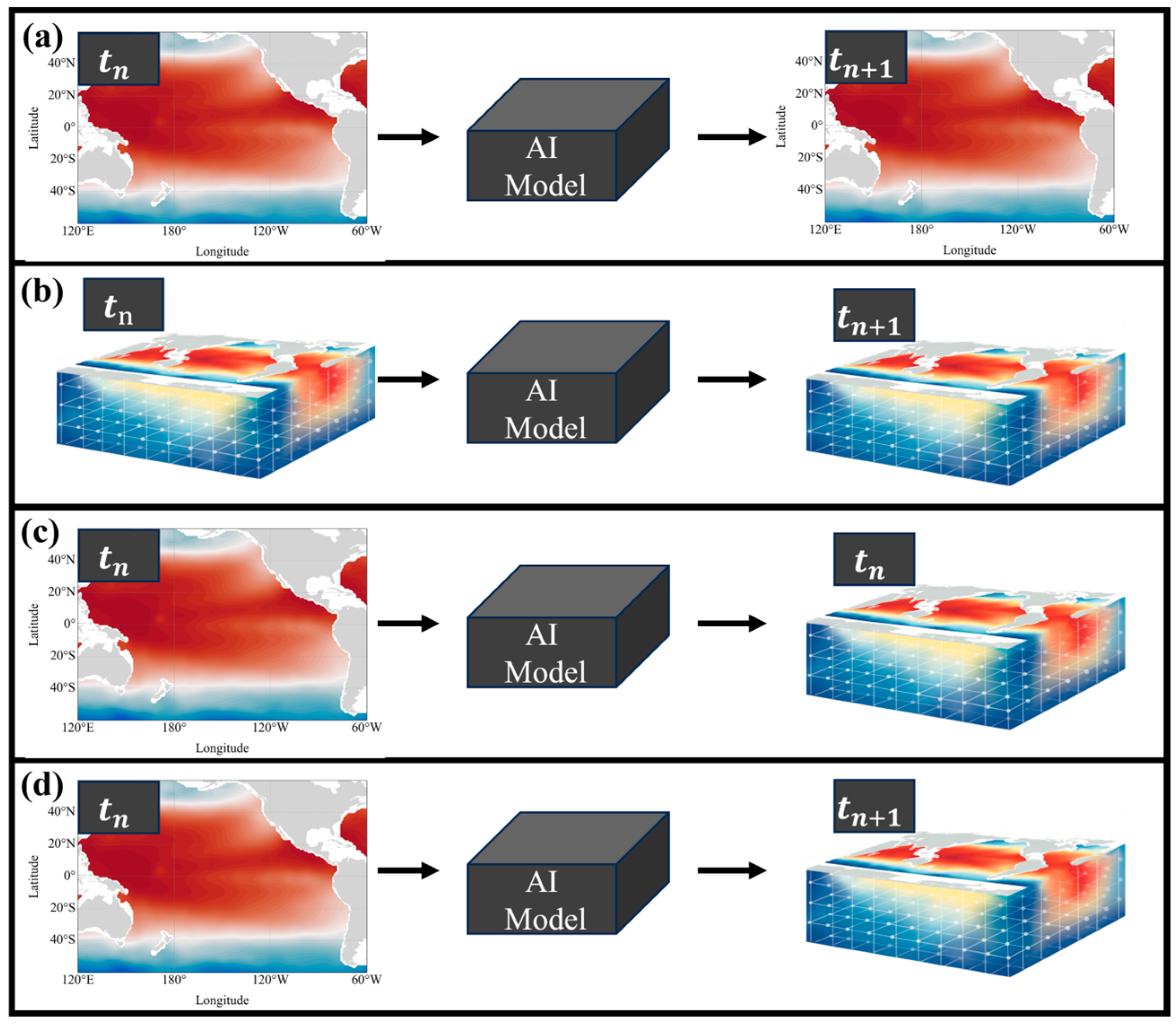
There are currently four major schemes for DORS work (Figure 1). Figure 1a shows the use of known satellite remote sensing data of the ocean surface to predict future changes at the ocean surface. For instance, Zhang et al. [18] employed the Long Short-Term Memory (LSTM) method to forecast sea surface temperature in offshore China, He et al. [19] developed the DSL method for predicting sea surface temperature, Zhang et al. [20] devised a U-Net method for time series prediction of sea surface salinity in the Western Pacific Ocean, Xu et al. [21] combined Memory in Memory (MIM) and Variational Mode Decomposition (VMD) to propose the VMD-MIM model, which further enhances the prediction performance of sea surface temperature. These approaches primarily focus on predicting surface changes, whereas subsurface data are often more valuable to researchers [22].
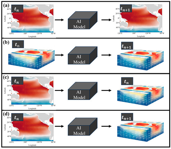
Figure 1.
(a) Surface ocean prediction using remote sensing images. (b) Subsurface ocean prediction using measured profile data. (c) Subsurface ocean reconstruction using satellite remote sensing images. (d) Subsurface ocean prediction using satellite remote sensing images.
Figure 1b depicts the use of historical subsurface three-dimensional structure data to forecast future subsurface changes. For example, Sun et al. [23] proposed a 3D U-Net model, utilizing the past 12 months of subsurface data to predict the subsurface structure for the next 12 months. Yue et al. [24] introduced the SA-PredRNN model, based on SA-ConvLSTM and PredRNN, to achieve similar predictions using historical subsurface data. Although these predictive models are valuable, they rely on extensive measured data as input, which poses practical limitations due to the data’s scarcity and acquisition challenges.
Figure 1c represents the most extensively studied approach, focusing on the reconstruction of subsurface ocean structures using remote sensing data. Su et al. [25] explored the reconstruction of subsurface temperature and salinity anomalies using machine learning methods such as Random Forest (RF) and Extreme Gradient Boosting (XGBoost), while Meng et al. [26] achieved high-resolution subsurface reconstruction through Convolutional Neural Networks (CNNs). Xie et al. [27] implemented subsurface reconstruction in the South China Sea region using a U-Net model based on convolutional neural networks. Recently, the introduction of the Transformer framework and attention mechanisms has facilitated the efficient reconstruction of subsurface structures by learning from historical data. For instance, Zhang et al. [28] developed a discrete point historical time series model to invert subsurface structures by capturing temporal changes, while Su et al. [29] utilized the Transformer framework to sample and extract spatial features from images of different scales, reducing computational costs and enabling efficient reconstruction of subsurface density fields. These methods, however, are focused on reconstruction and do not predict future subsurface structures.
Figure 1d illustrates the relatively novel approach of using historical remote sensing data to predict future subsurface changes in the ocean. In 2024, Liu et al. [22] introduced an artificial intelligence model that employed historical remote sensing images to forecast future subsurface ocean structures, training the model with satellite remote sensing and numerical simulation data, and achieving notable results in the South China Sea region.
By comparing these DORS methods, we identify several pertinent questions for further exploration: (1) Is there a performance difference between using historical remote sensing data to predict future subsurface ocean profile structures and using historical subsurface ocean profile structures for the same purpose? (2) What is the relationship between the reconstruction of subsurface structures that combines historical and real-time data, and the prediction of subsurface structures using only historical data?
In this paper, we propose the multiscale spatiotemporal window ocean (MSWO) model, which combines the features of the spatiotemporal series network SimVP [30] and the computer vision Swin Transformer [31] network. The MSWO model employs a window attention mechanism in the spatiotemporal dimension to achieve low computational-load attention effects. Additionally, it extracts the nonlinear spatiotemporal relationships in the data through multi-scale residuals. To better represent the spatial and temporal characteristics of the data, we introduce global location coding during information extraction and use the channel attention mechanism to extract key feature information from remote sensing images. The model was validated against measured Argo grid data in the Central South Pacific. Historical remote sensing data from the past 24 months were used to predict the subsurface temperature structure trends in the Central South Pacific for the next 6 months. Furthermore, we explored the effect of using measured profile structures from the past 24 months to predict the subsurface structure for the next 6 months, comparing the reconstructed results with the predicted results on the test dataset. The results indicate that our model achieves the highest inversion accuracy in both reconstruction and prediction processes. This method presents a promising new approach for transparent ocean observation.
2. Related Work
Both the reconstruction of ocean subsurface structures and the prediction of future subsurface changes can be accomplished using spatiotemporal series models. With the development of artificial intelligence, more and more remote sensing images are used to reconstruct ocean subsurface structures and begin to invert historical data as one of the input factors [28,29].
Spatiotemporal series models have their origins in single-element time series prediction models, with the most traditional method being the recurrent neural networks (RNNs). The LSTM [32] subsequently improved the model’s efficiency in learning temporal patterns. In 2015, Shi et al. [33] advanced this field by introducing the ConvLSTM model, which replaced the fully connected layer with a convolutional layer in the FC-LSTM, marking a transition from time series models to spatiotemporal series models. This innovation extended LSTM input data to multidimensional images, maintaining the fundamental principles of LSTM and other recurrent neural networks. The prediction for the next time point is achieved by iterating through the forgetting gate, output gate, and memory cell. In 2017, Wang et al. [34] proposed PredRNN, based on ConvLSTM, which introduced a long-term memory module to enhance the accuracy of spatiotemporal series prediction tasks.
The introduction of the attention mechanism and the Transformer framework [35] in 2017 revolutionized natural language-processing research. Researchers discovered that the attention mechanism’s ability to capture global changes was superior to that of convolutional neural networks, leading to its application in computer vision. Various Transformer framework variants [31,36,37,38] have since achieved remarkable success in object detection, image classification, and semantic segmentation. The attention mechanism’s capability to capture global information has also been applied to time series prediction tasks [39,40]. In 2020, Lin et al. [41] incorporated the self-attention module into the ConvLSTM model, resulting in the SA-ConvLSTM model, which can capture global spatiotemporal correlations. However, with higher-resolution image inputs, spatiotemporal series prediction models faced similar computational cost challenges as those in computer vision. The Swin Transformer [31] improved model performance while significantly reducing computational complexity. Consequently, in 2023, Tang et al. [42] replaced the convolutional layer in ConvLSTM with the Swin Transformer, achieving optimal results on video prediction datasets such as Moving MINST.
However, the iterative RNN-based spatiotemporal series models have inherent flaws. As illustrated in Figure 2a, the prediction for the current time step in an iterative model is influenced by the previous time step’s prediction, leading to error accumulation over time. Additionally, this process tends to make the model overly reliant on immediate past context information, hindering long-term information learning [43]. To address this issue, various generative models have been developed to generate all prediction results by capturing global information in a single step [39,44], as shown in Figure 2b. In 2023, Tan et al. [30] proposed the SimVP model, which uses an Encoder–Decoder architecture for feature extraction and large-kernel convolution to simulate a global attention mechanism, achieving excellent results in spatiotemporal prediction. With the advent of a new generation of satellites, remote sensing images now feature larger scales and higher resolutions. Consequently, the primary objective of this paper is to design an efficient artificial intelligence model that supports high-resolution images to predict the future three-dimensional structure of the ocean.
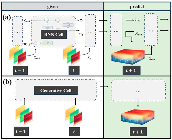
Figure 2.
(a) Flow chart of RNN iterative framework on spatiotemporal prediction tasks. (b) Flow chart of the generative framework for spatiotemporal prediction tasks.
3. Method
3.1. Overall Architecture
The MSWO model aims to design an autoencoder architecture suitable for spatiotemporal sequence prediction tasks, and predicts future images based on the learning of past temporal related frames. Different from the traditional iterative RNN, the MSWO model uses a generative strategy. The traditional automatic encoder generates a single step frame in static time and minimizes the difference between the true probability distribution and the predicted probability distribution by mapping . The optimal parametric neural network is as follows:
where Div represents a specific loss function. Similarly, MSWO encodes the frames of the entire historical time dimension, decodes the future prediction time dimension, and minimizes the difference between the predicted and true probability distributions by mapping . The optimal parametric neural network is:
In the experiment, we choose the loss function to minimize the error between this mapping:
3.2. MSWO Module
Assuming that the size of the input remote sensing image is in times, represents the length of the image, represents the width of the image, and represents the number of channels of the image, the entire input can be represented by a tensor . As shown in Figure 3, the input shape is , where B represents batch size. The whole MSWO model consists of three parts: spatial encoder, window attention, and spatial decoder.
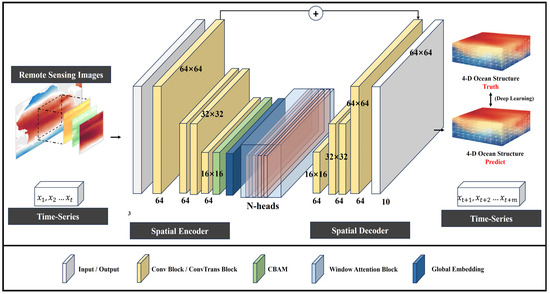
Figure 3.
Flow diagram of MSWO using satellite remote sensing data to predict subsurface ocean temperature structure. 4-D represents the xyz axis in the time dimension and space.
The spatial encoder consists of two subsampled convolution layers, the convolutional block attention module (CBAM) [45], global attention coding [46], and residual concatenation. By stacking convolution layers, high-dimensional satellite remote sensing images are encoded into the low-dimensional potential space as follows:
where represents the activation function used to extract nonlinear variations from features, and is the normalization layer. CBAM includes a channel attention module and a spatial attention module, which use average pooling and max pooling methods to extract useful channel information and spatial information, helping the model to better learn critical information and enhance sensitivity, thereby improving the overall performance of the model.
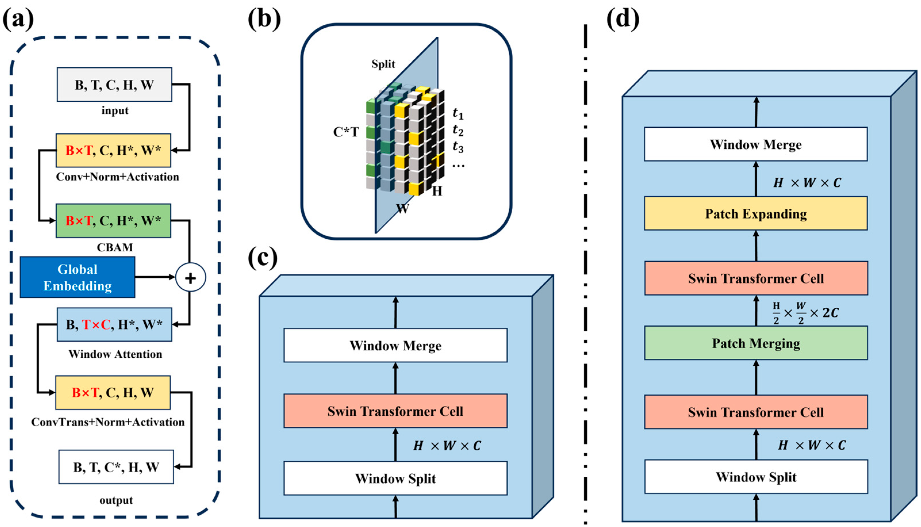
After spatial encoder, we reshape the dimensions of the tensor as . The purpose of this is to stack the single frame images at different times along the time axis and update the channel of the image to the combination of the doped time dimension. The tensor is then entered into the window attention module. For large-scale and high-resolution spatiotemporal series prediction tasks, the computational complexity of global attention is generally , and the spatial complexity is . Such square-level computational complexity causes a very large load on intensive prediction tasks [36]. By stacking time dimension and channel dimension, MSWO controls the matrix multiplication operation in smaller dimensions. The overall computational complexity of the model is , and the space complexity becomes , which greatly reduces the overhead of the model. In addition, inspired by the Swin Transformer [35] and SwinLSTM [40] models, we designed SWO and MSWO options in the window attention section, as shown in Figure 4c,d. SWO includes general window segmentation and a sliding window module. By dividing the whole image and performing attention calculation in the window, the computing overhead is further reduced. At this time, the whole image is divided into window matrices of size, and the computational complexity is reduced to , and the space complexity is . In MSWO, we use patch merging to acquire multi-scale image data, and through the residual joining operation, we can focus on a larger sensory field in the size window.
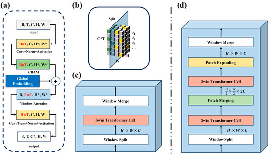
Figure 4.
Details in the MSWO process. (a) The process of tensor dimension change in the whole process. (b) Window segmentation and attention calculation diagram. (c) SWO model flow chart. (d) MSWO model flow chart.
The Swin transformer cell is divided into two modules. The first module captures the token relationship inside the window through the window-multi-head attention mechanism (W-MHA); the second module is the same as the first module, only the W-MHA is replaced by the shift window-multi-head attention (SW-MHA) to capture the token relationship between adjacent windows. Finally, the decoding process also needs to reshape the tensor shape into to extract the information of a single image, and map the subsampled spatiotemporal data back to the original size through a deconvolution operation as follows:
4. Experiments
In the experimental part, we introduce the whole experimental design of the model, including data sources, processing methods, parameters of the training model, evaluation indexes of the model results, and the design of the ablation experiment.
4.1. Data
In this study, we utilized globally available datasets, including sea surface temperature (SST), absolute dynamic topography (ADT), sea surface salinity (SSS), and Argo-measured datasets. The temporal resolution for all data is monthly averages, and the spatial resolution was interpolated to 1° × 1° using interpolation methods. During the training and testing phases, satellite remote sensing data were integrated as input variables, and Argo profile data served as output variables. As detailed in Table 1, SST data were sourced from the National Oceanic and Atmospheric Administration (NOAA)’s OISST dataset, ADT data from Aviso, and SSS data from SMOS satellite’s Level 3 data. The study area encompassed the Central South Pacific, spanning from 44.5°S to 18.5°N and 116.5°W to 179.5°W. The input dimensions for the remote sensing images were 64 × 64 pixels. The temporal sequence of the dataset ranged from January 2011 to December 2019, encompassing 108 months. The time series data were divided into training, validation, and testing sets in a 7:1:1 ratio, employing a sliding window method [39]. The input time series covered 24 months, with predictions extending 6 months into the future. Argo depth selection focused on the upper 250 m of the ocean, divided into 10 depth layers (10, 20, 30, 50, 75, 100, 125, 150, 200, and 250 m). Outlier data were processed and optimally interpolated, and the following method was used for data normalization:

Table 1.
Data sources and resolutions used in present study.
The MSWO model was implemented using the PyTorch framework. The training process utilized the loss function and the Adam optimizer with a learning rate of 0.001. The model was trained for 1000 epochs, with an early stopping criterion set at 50 epochs, and a batch size of 2. To ensure robustness of the final results, all experiments were repeated three times on an Nvidia Tesla V100 GPU, with the mean and standard deviation of these repetitions reported as the final results.
4.2. Evaluation Indicator
We used three evaluation metrics to evaluate the performance of the predicted results against the measured results, which are mean square error (MSE), root mean square error (RMSE), and mean absolute error (MAE). These three indicators are used to measure the correlation between two data vectors, and the calculation process is as follows:
5. Result and Discussion
In this study, we primarily explored the performance of the MSWO model and its capability to predict future changes in ocean subsurface structures using remote sensing satellite images. Under limited training data conditions, the MSWO achieved optimal prediction accuracy. Furthermore, we compared the prediction model with the ocean subsurface structure reconstruction model. Over the 12 months of the test dataset, the prediction and reconstruction models exhibited complementary trends in model accuracy, which may offer new insights for future research.
5.1. Results of Ablation Experiment
The selection of different modules or methods can significantly impact the performance of the MSWO model. In the ablation study section, we investigated the performance of the SWO and MSWO models when incorporating global encoding and the shift window mechanism. Compared to the SWO model, the MSWO model employs the same down-sampling and up-sampling mechanisms as the SwinLSTM model, capturing larger-scale spatial processes by resizing the entire image. Additionally, unlike the spatial relative position encoding used in the window attention mechanism, the global encoding is introduced before the window attention layer. This global encoding allows elements within each small window to not only focus on elements within the same window but also to consider the global context. The shift window mechanism supplements the attention relationships between adjacent independent windows, aligning with the approach proposed by the Swin Transformer. The results of all ablation experiments are shown in Table 2. Overall, using down sampling to capture large-scale spatial information and introducing global spatiotemporal encoding enhances model accuracy. The best SWO model achieved an average MSE of 0.661, RMSE of 0.757, and MAE of 0.528 on the test dataset, while the best SWO-D model achieved an average MSE of 0.648, RMSE of 0.749, and MAE of 0.516 on the test dataset. For convenience, the SWO and MSWO models referred to in the following sections are the best-performing models.
Table 2.
The results of ablation experiments are recorded, and the Model includes SWO and MSWO; Global represents whether global encoding of space-time was introduced, and Shifted represents whether a shifted window mechanism was used. The bold part represents the group with the best performance in the SWO and MSWO models.
5.2. Model Comparison
In the field of spatiotemporal prediction, numerous advanced artificial intelligence models have been proposed for tasks such as video prediction and weather forecasting. Similar to these works, we utilized these established spatiotemporal sequence models as baseline models to evaluate the performance of the MSWO model. The baseline models include ConvLSTM, PredRNN, SwinLSTM, EarthFormer, SA-ConvLSTM, and SimVP. The input and output formats for MSWO were kept consistent with these baseline models, and the accuracy of the predictions was evaluated using MSE, RMSE, and MAE metrics. To further reduce the likelihood of random events, all experiments were repeated three times, with the mean and the standard deviation recorded for each experiment. Each training and testing session was conducted on an Nvidia Tesla V100 GPU. The average results obtained from all baseline models are presented in Table 3. The overall mean MSE for ConvLSTM, PredRNN, SwinLSTM, EarthFormer, SA-ConvLSTM, SimVP, and our MSWO model was 0.829, 1.007, 1.074, 0.789, 0.935, 0.768, 0.661, and 0.648, respectively. The overall mean RMSE was 0.858, 0.925, 0.963, 0.834, 0.891, 0.813, 0.757, and 0.749, respectively. The overall mean MAE was 0.580, 0.634, 0.648, 0.596, 0.610, 0.575, 0.528, and 0.516, respectively. The MSWO model achieved the best predictive accuracy among all the compared models, indicating its advantage in predicting changes in ocean subsurface structures. This demonstrates that the MSWO model has superior predictive performance in this domain.
Table 3.
Comprehensive prediction comparison results between the SWO model and other baseline models on the test dataset, where Size represents the size of the image in the calculation process, and EarthFormer and MSWO perform multi-resolution sampling operations, respectively. The bold part represents the group with the best performance in different model experiments.
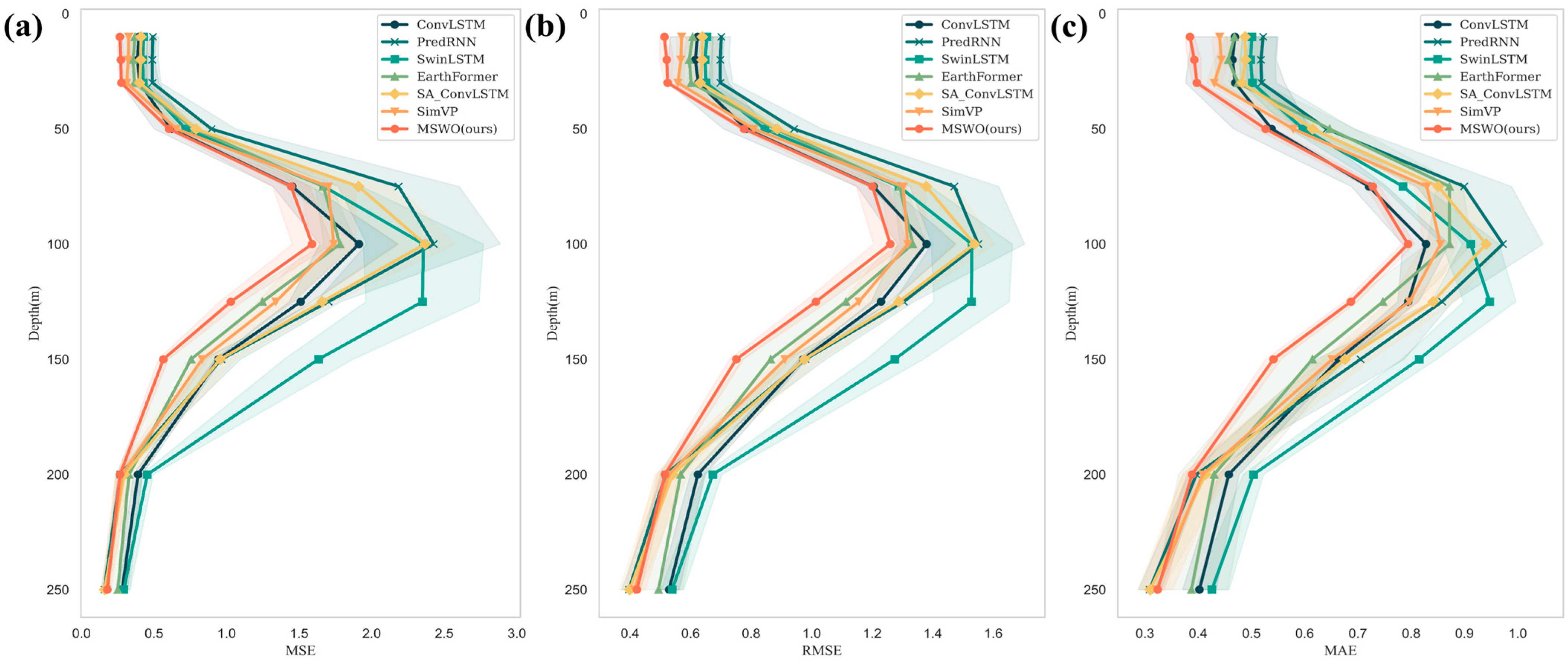
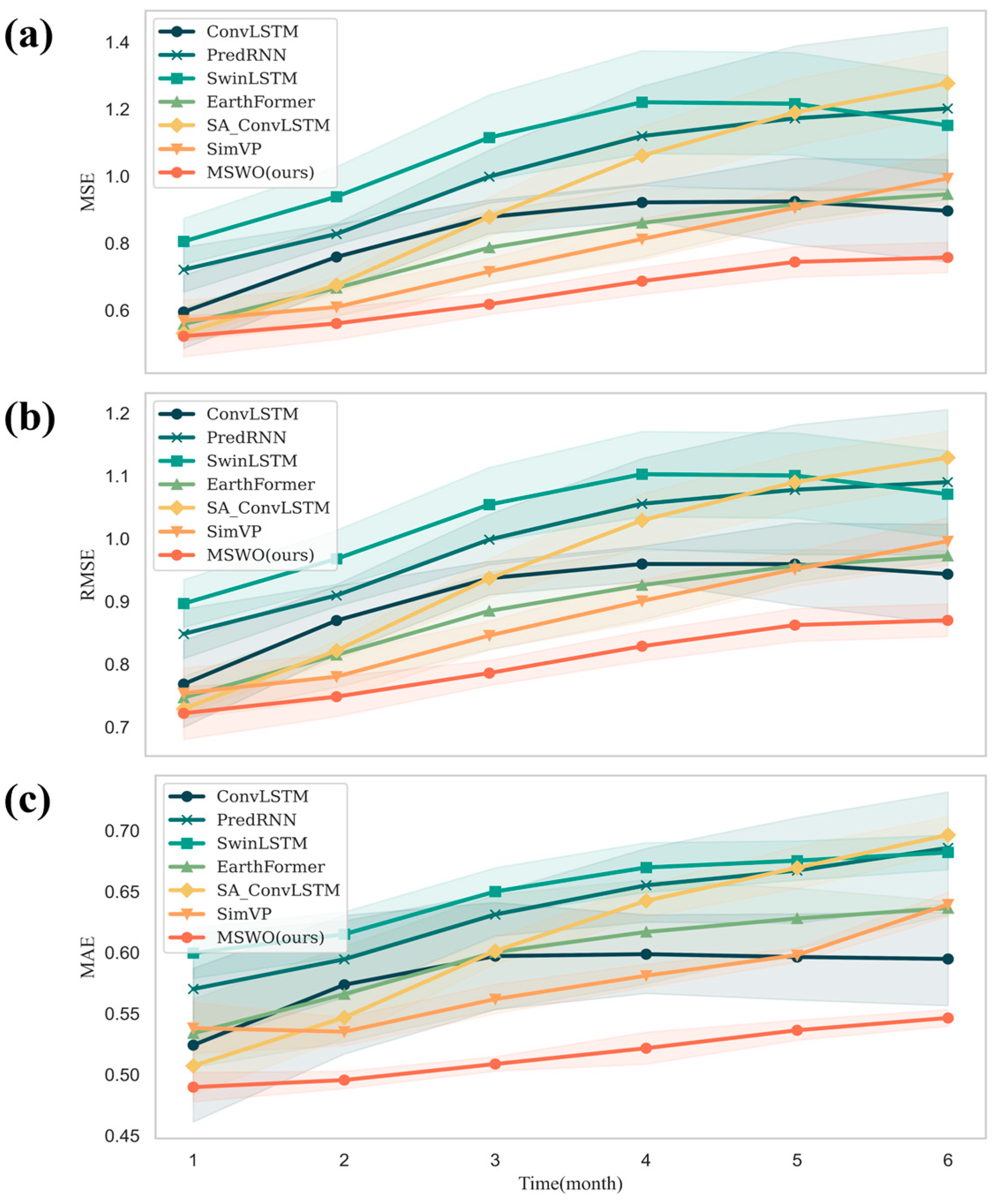
To illustrate the variations in predictive accuracy over space and time, we have plotted Figure 5 and Figure 6. Figure 5 presents the performance metrics of different models at various depths within the upper 250 m of the ocean, while Figure 6 shows the performance metrics across different months. All models exhibited a trend where the prediction error initially increases and then decreases, with the maximum error occurring around the 100 m depth. This corresponds to the thermocline, a transitional layer between warmer surface water and cooler deep water, characterized by a steep vertical temperature gradient. The thermocline significantly affects the ocean’s density and acoustic fields. Numerous previous studies [22,29,47,48] have highlighted the challenges artificial intelligence models face in accurately reconstructing subsurface structures due to the presence of the thermocline, posing a considerable challenge for all predictive tasks. For the study area, another challenge is the irregular variations in ocean structure caused by the El Niño–Southern Oscillation (ENSO) phenomenon. The limited availability of measured data hampers the ability of AI models to learn long-term decadal variations, thus obstructing accurate future predictions. Figure 6 shows how model errors change over time, with almost all models displaying an increase in error as the prediction horizon extends. This error increase is due to both the declining correlation between the output results and the real satellite data inputs, as well as the accumulation of errors from the recursive process. Overall, the MSWO model achieved the best predictive performance among all compared models, with the lowest error increase over time. This demonstrates that the MSWO model has broad application potential in the field of spatiotemporal sequence prediction.
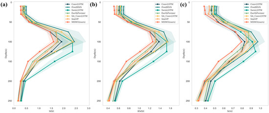
Figure 5.
Evaluation index results of different models at different depths. (a) MSE, (b) RMSE, (c) MAE.
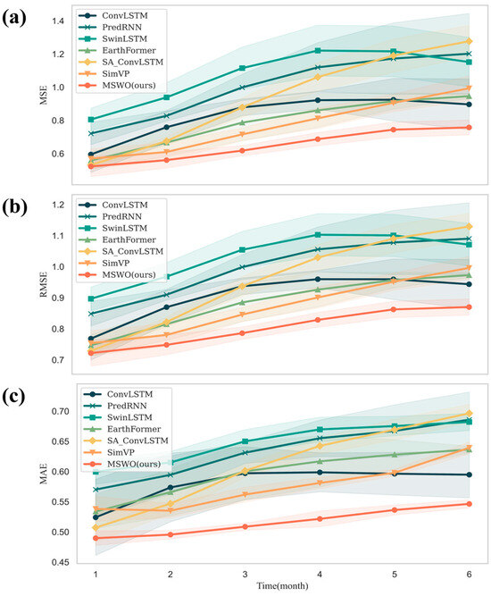
Figure 6.
Evaluation index results of different models in the predicted 6-month period. (a) MSE, (b) RMSE, (c) MAE.
5.3. Compare with P2P Schemes
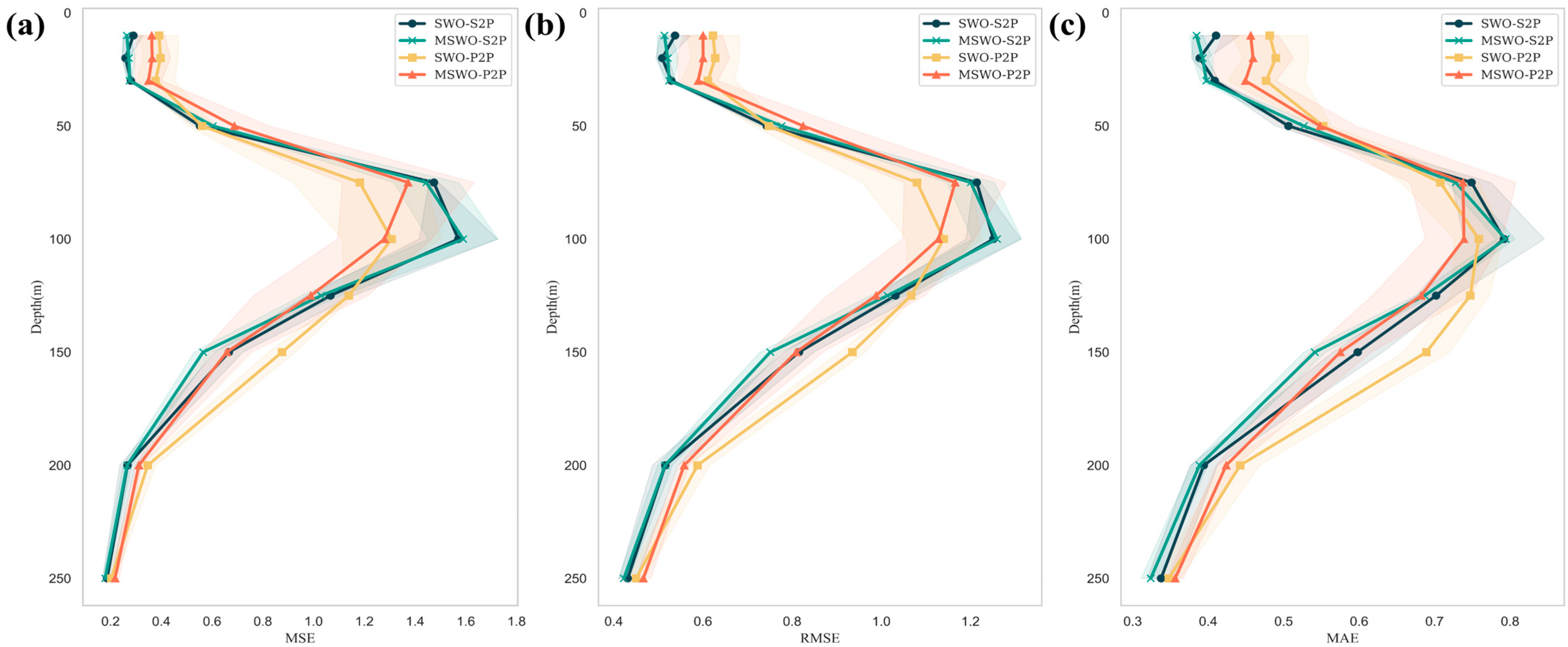
In this study, we introduce a method for predicting future subsurface ocean temperature structures using historical satellite remote sensing images. However, we pose a new inquiry: How does the performance of using satellite remote sensing imagery as input for prediction compare to using historical profile data? Employing satellite remote sensing image for predicting future ocean structures is more convenient due to its lower cost of acquisition, wider coverage, and longer available period. Hence, we replaced historical satellite remote sensing data with historical measured Argo data as input, employing the MSWO model for training and testing. The experiments were replicated three times on an Nvidia Tesla V100 GPU, utilizing MSE, RMSE, and MAE as evaluation metrics. The performance of the model across depths is depicted in Figure 7.
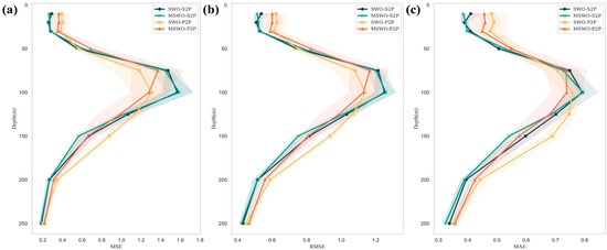
Figure 7.
Evaluation index results of historical satellite remote sensing predicting future profile structure (S2P) and historical profile predicting future profile structure (P2P) models at different depths. (a) MSE, (b) RMSE, (c) MAE.
In Figure 7, S2P (surface to profile) and P2P (profile to profile) represent predictions of future profile structures using historical satellite remote sensing and historical profile data, respectively. Unexpectedly, compared to using solely satellite remote sensing data, employing larger volumes of historical profile data did not result in a significant increase in predictive accuracy; the predictive errors of P2P remained largely comparable to those of S2P. A comparison between the S2P and P2P modes reveals the superior performance of S2P in the upper layers of the ocean and the relatively better results around 100 m depth for P2P. This suggests that variations captured by satellite remote sensing data exhibit more relevant features in the prediction process for upper ocean layers. As the inversion depth increases, the introduction of historical profile data may lead to improved inversion outcomes. Overall, the comprehensive performance of S2P and P2P modes in this experiment did not demonstrate significant differences. This finding may be attributed to the fact that changes in the upper 250 m of ocean structure are largely influenced by surface ocean dynamics, and the variations captured by historical satellite remote sensing data are already sufficiently comprehensive. Despite being influenced by dataset limitations and variations related to ENSO phenomena in the study area, predictive models still have considerable room for improvement in accuracy. Nevertheless, this discovery underscores the efficacy of utilizing historical satellite remote sensing data for predicting future subsurface ocean structures, with an accuracy comparable to using historically measured data for forecasting future ocean profiles. This facilitates the direct utilization of satellite remote sensing imagery for large-scale, long-term prediction forecasts in practical applications.
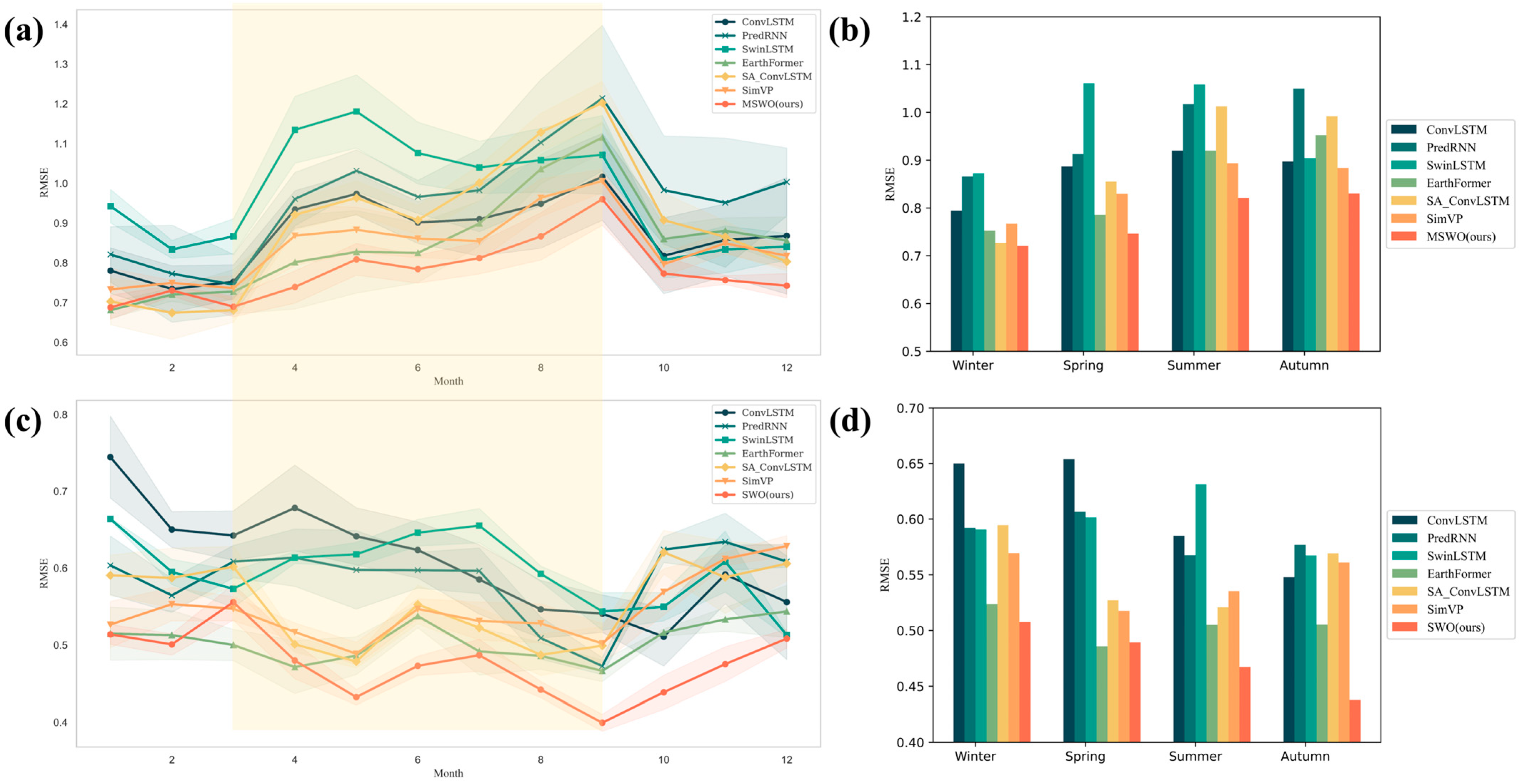
The task of predicting the next 6 months using the preceding 24 months differs from the reconstruction task, where the input comprises the preceding 12 months’ data alongside the known 6 months’ data to reconstruct the subsurface ocean temperature structure. In contrast to future prediction tasks, reconstruction tasks benefit from the utilization of real-time satellite remote sensing data, enabling them to better capture real-time changes while learning historical patterns. To examine the similarities and differences in the inversion results between the two approaches, we conducted a comparative analysis between the prediction and reconstruction results. Specifically, we divided the test set into 12 months, which were then categorized into four seasons based on the Northern Hemisphere’s months (with December to February categorized as spring, March to May as summer, June to August as autumn, and September to November as winter), as depicted in Figure 8. Figure 8a represents the prediction results for the 12 months of 2019 obtained by different models using the prediction method, with the line graph illustrating the RMSE between predicted and actual values. Figure 8c depicts the reconstruction results for the 12 months of 2019 obtained by different models using the reconstruction method, with the line graph showing the RMSE between reconstructed and actual values. Figure 8b,d showcase the seasonal variation in errors across different models.

Figure 8.
(a) RMSE changes of different baseline models on the 12-month prediction task of the test dataset. (b) Seasonal RMSE bar chart of different benchmark models on the prediction task of the test dataset. (c) RMSE changes for different baseline models on 12-month reconstruction tasks of the test dataset. (d) Seasonal RMSE histogram for different benchmark models on the reconstruction task of the test dataset.
From Figure 8, it is evident that the prediction models generally exhibit higher errors compared to the reconstruction models. Interestingly, we observe an inverse trend in inversion errors between the prediction and reconstruction models on the test dataset (highlighted in the yellow box in the figure). We attribute this phenomenon to the prediction models primarily learning regularities on the temporal scale, lacking input of real-time spatial change data. In contrast, the reconstruction task for subsurface ocean structure better addresses this gap, optimizing inversion results further by incorporating real-time satellite remote sensing data onto the foundation of spatiotemporal sequence prediction. This holds practical significance, particularly for real-time forecasting endeavors.
5.4. Section Cutting Comparison
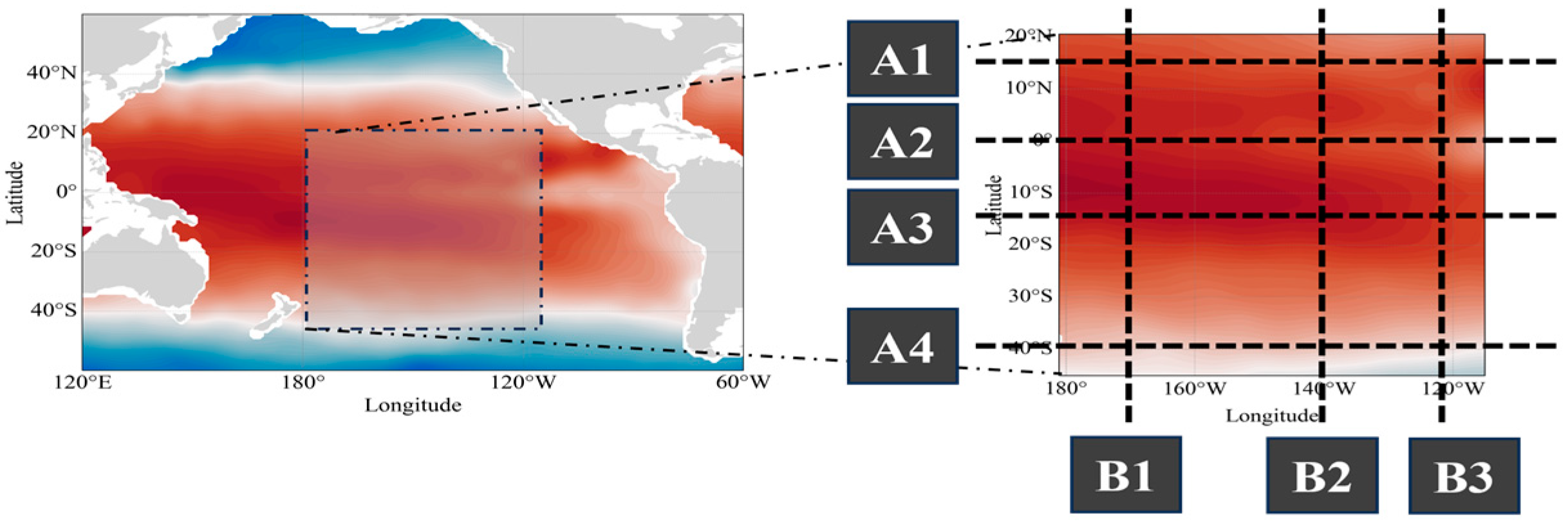
To further validate the consistency between the three-dimensional subsurface ocean structure predicted by MSWO and the measured data, we selected four latitudinal and three longitudinal transects for cross-sectional plotting. As shown in Figure 9, along the latitude direction, we selected four transects at 15.5°N (A1), 0.5°N (A2), 15.5°S (A3), and 40.5°S (A4), while along the longitude direction, we chose three transects at 169.5°W (B1), 139.5°W (B2), and 119.5°W (B3). We present the measured Argo profiles, predicted profiles, and their differences plotted along these transects using the MSWO model on the test dataset for January 2019, as illustrated in Figure 10 and Figure 11.

Figure 9.
Section selection diagram.
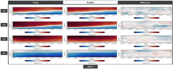
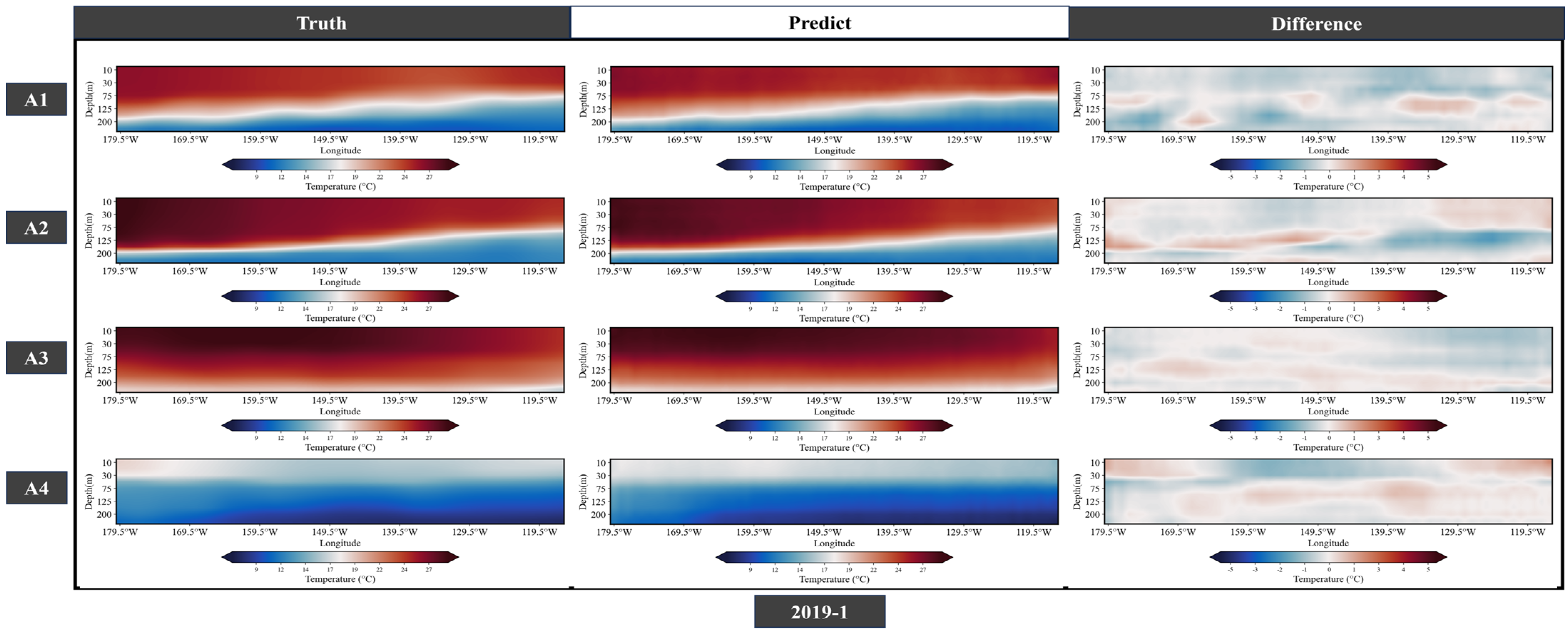
Figure 10.
Profile diagram of the January 2019 test dataset drawn at A1–A4 cross sections.
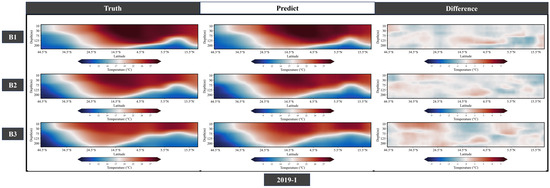
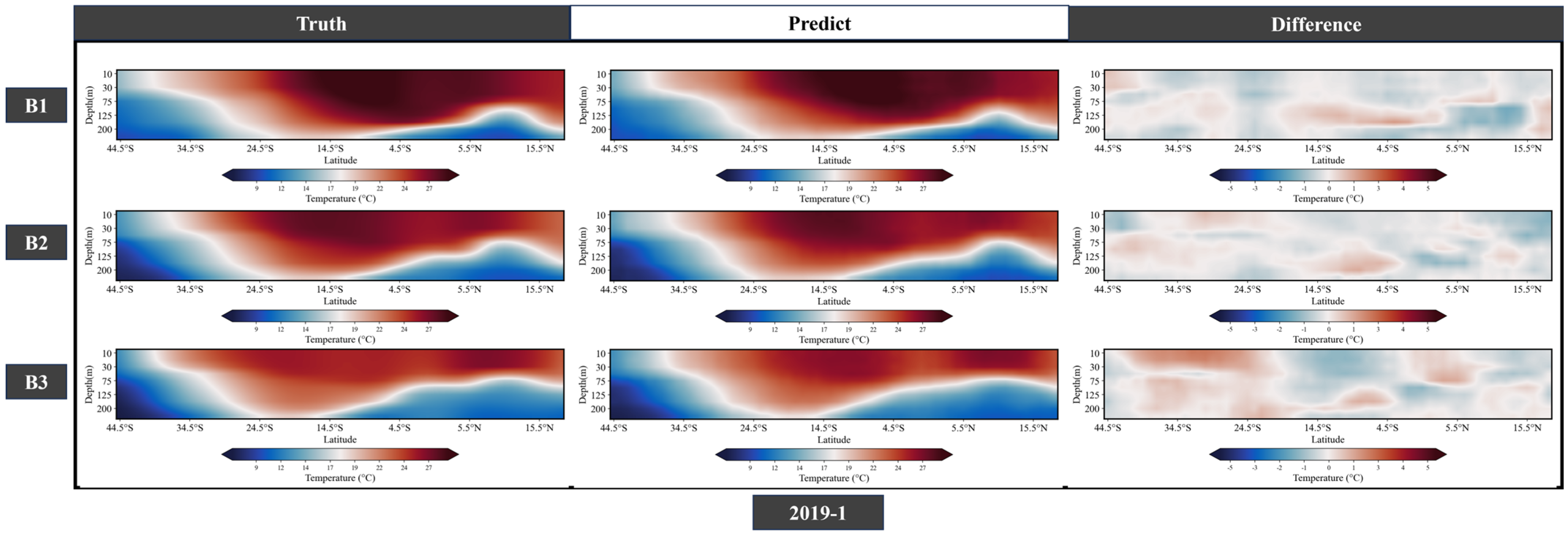
Figure 11.
Profile diagram of the January 2019 test dataset drawn at B1–B3 cross sections.
Observing the relationship between the measured and true profiles in Figure 10, it is evident that near the equator, warm water driven by the easterly winds converges into the western Pacific warm pool before sinking, leading to a gradient distribution in subsurface temperatures and shallower thermoclines in the eastern Pacific and deeper thermoclines in the western Pacific. Compared to the measured data, the predicted results from the MSWO model also reflect these gradient changes. Similarly, examining the relationship between the measured profiles in Figure 11, it is observed that the subsurface temperatures in the warm pool region near the equator are higher than those in the eastern Pacific, and subsurface temperatures in the low latitudes of the South Pacific are higher than those in the North Pacific. This distribution correlates strongly with the South Equatorial Current (SEC), Equatorial Under Current (EUC), North Equatorial Counter Current (NECC), and North Equatorial Current (NEC) [49], indicating that MSWO can effectively predict changes in subsurface water masses within the ocean.
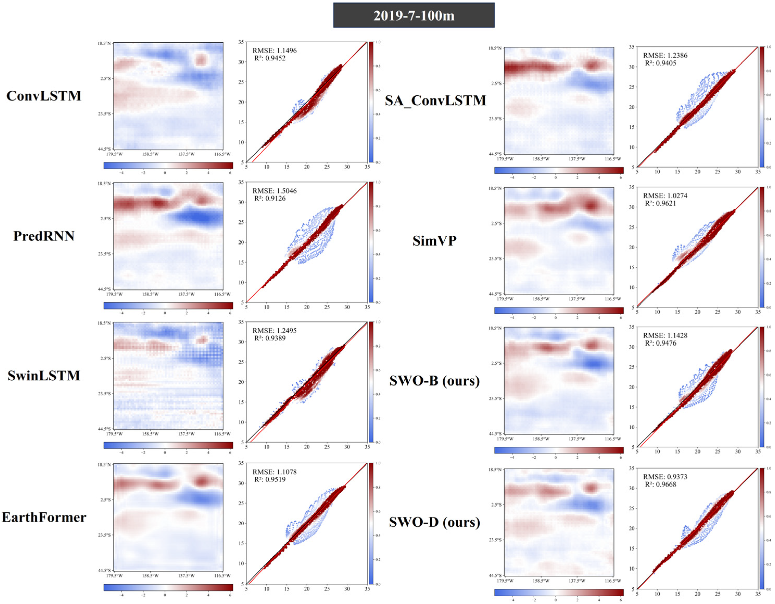
5.5. Planar Error and Density Scatter
The planar error facilitates an understanding of the distribution of errors between the predicted results and the measured data, while the density scatter plot evaluates the correlation between the measured values and the model’s predicted results, as well as the robustness of the model’s performance. Thus, we generated planar error maps and density scatter plots for all baseline models in July 2019, focusing on the upper 100 m of the ocean. As depicted in Figure 12, significant errors were observed near the equator across all models, with the eastern Pacific displaying underestimations and the western Pacific showing overestimations, a pattern closely associated with the 2019 El Niño event. Overall, MSWO exhibited favorable performance advantages in predicting the development and changes in subsurface oceanic structures. Furthermore, compared to other baseline models, MSWO demonstrated the best robustness and most concentrated inversion effects in the density scatter plot.
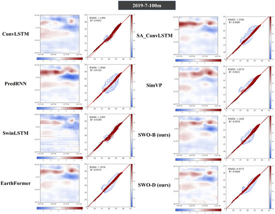
Figure 12.
All baseline models were compared with the MSWO model for planar error plots and density scatter plots.
6. Conclusions
With the advancement of human science, the development of artificial intelligence technology has gradually provided new methods and perspectives for realizing the strategy of transparent oceans. In this paper, we proposed the MSWO model and employed it to predict the subsurface temperature structure for the next six months in the Central South Pacific region using satellite remote sensing data from the past 24 months. MSWO introduces a global positional encoding to enrich the spatiotemporal relationship features among the data and utilizes channel attention mechanisms to extract crucial information. Subsequently, MSWO employs multiscale residual operations and window attention mechanisms to extract spatiotemporal correlations within the input data, facilitating predictions of future subsurface oceanic structures. In comparative experiments, MSWO achieved the best predictive performance, benefiting from the attention mechanism’s extraction of global spatiotemporal information and its efficient utilization. Additionally, we explored the impact of using either satellite remote sensing data alone or profile data alone as inputs on future predictions. Surprisingly, the results from both strategies were similar, indicating that we can directly predict and forecast future oceanic changes using satellite remote sensing methods, which are more practically applicable compared to profile prediction models that require scarce measured data. Furthermore, we compared the performance of MSWO in prediction tasks and reconstruction tasks. The experimental results show that the error trends of prediction models and reconstruction models exhibited complementary characteristics across the 12 months of the test dataset. The incorporation of remote sensing images as inputs in reconstruction models further complements the real-time features missing in prediction models, thereby improving inversion accuracy.
However, there are still many opportunities for further development in this research. For instance, the lack of measured datasets limits the model’s ability to capture long-term decadal changes, and the monthly and spatial resolutions lead to the loss of many small and medium-scale change processes. The impact of the ENSO process on the model cannot be avoided, and the extent of its influence is currently unclear. The design of the MSWO model supports high-resolution satellite remote sensing images and large-scale spatiotemporal process forecasting. In future work, we will explore higher-resolution ocean reconstruction and forecasting.
Author Contributions
Conceptualization, L.W. and X.Z.; Data curation, Y.L.; Formal analysis, J.W.; Investigation, J.J.; Methodology, J.J.; Resources, X.Z.; Supervision, X.Z.; Validation, J.J., C.H. and Q.J.; Visualization, L.F. All authors have read and agreed to the published version of the manuscript.
Funding
This work was supported by the Technology Support Talent Program of the Chinese Academy of Sciences (E4KY31), the Chinese Academy of Sciences pilot project (XDB42000000), the Major Science and Technology Infrastructure Maintenance and Reconstruction Project of the Chinese Academy of Sciences (DSS-WXGZ-2022), the National Key Research and Development Program (2021YFC3101504), the National Natural Science Foundation of China (42176030) and High Level Innovative Talent Project of NUDT.
Data Availability Statement
The Argo data can be downloaded from http://apdrc.soest.hawaii.edu/projects/Argo/ (accessed on 1 May 2024); the ADT data can be downloaded from https://www.aviso.altimetry.fr/en/data/products/ (accessed on 1 May 2024); the SST data can be downloaded from https://climatedataguide.ucar.edu/climate-data/sst-data-noaa-high-resolution-025x025-blended-analysis-daily-sst-and-ice-oisstv2 (accessed on 1 May 2024); and the SSS data can be downloaded from https://www.catds.fr/Products/Catalogue-CPDC/Catds-products-from-Sextant#/metadata/0f02fc28-cb86-4c44-89f3-ee7df6177e7b (accessed on 1 May 2024).
Conflicts of Interest
The authors declare no conflicts of interest.
References
- Behrenfeld, M.J.; O’Malley, R.T.; Siegel, D.A.; McClain, C.R.; Sarmiento, J.L.; Feldman, G.C.; Milligan, A.J.; Falkowski, P.G.; Letelier, R.M.; Boss, E.S. Climate-Driven Trends in Contemporary Ocean Productivity. Nature 2006, 444, 752–755. [Google Scholar] [CrossRef] [PubMed]
- Johnson, G.C.; Lyman, J.M. Warming Trends Increasingly Dominate Global Ocean. Nat. Clim. Change 2020, 10, 757–761. [Google Scholar] [CrossRef]
- Lowman, H.E.; Emery, K.A.; Dugan, J.E.; Miller, R.J. Nutritional Quality of Giant Kelp Declines Due to Warming Ocean Temperatures. Oikos 2022, 2022. [Google Scholar] [CrossRef]
- Cheng, L.; Abraham, J.; Zhu, J.; Trenberth, K.E.; Fasullo, J.; Boyer, T.; Locarnini, R.; Zhang, B.; Yu, F.; Wan, L.; et al. Record-Setting Ocean Warmth Continued in 2019. Adv. Atmos. Sci. 2020, 37, 137–142. [Google Scholar] [CrossRef]
- Li, J.; Sun, L.; Yang, Y.; Yan, H.; Liu, S. Upper Ocean Responses to Binary Typhoons in the Nearshore and Offshore Areas of Northern South China Sea: A Comparison Study. Coas 2020, 99, 115–125. [Google Scholar] [CrossRef]
- Chassignet, E.P.; Hurlburt, H.E.; Smedstad, O.M.; Halliwell, G.R.; Hogan, P.J.; Wallcraft, A.J.; Baraille, R.; Bleck, R. The HYCOM (HYbrid Coordinate Ocean Model) Data Assimilative System. J. Mar. Syst. 2007, 65, 60–83. [Google Scholar] [CrossRef]
- Chen, C.; Liu, H.; Beardsley, R.C. An Unstructured Grid, Finite-Volume, Three-Dimensional, Primitive Equations Ocean Model: Application to Coastal Ocean and Estuaries. J. Atmos. Ocean. Technol. 2003, 20, 159–186. [Google Scholar] [CrossRef]
- Meng, Y.; Rigall, E.; Chen, X.; Gao, F.; Dong, J.; Chen, S. Physics-Guided Generative Adversarial Networks for Sea Subsurface Temperature Prediction. IEEE Trans. Neural Netw. Learn. Syst. 2023, 34, 3357–3370. [Google Scholar] [CrossRef] [PubMed]
- Wang, J.; Ma, Q.; Wang, F.; Lu, Y.; Pratt, L.J. Seasonal Variation of the Deep Limb of the Pacific Meridional Overturning Circulation at Yap-Mariana Junction. JGR Ocean. 2020, 125, e2019JC016017. [Google Scholar] [CrossRef]
- Liu, C.; Feng, L.; Köhl, A.; Liu, Z.; Wang, F. Wave, Vortex and Wave-Vortex Dipole (Instability Wave): Three Flavors of the Intra-Seasonal Variability of the North Equatorial Undercurrent. Geophys. Res. Lett. 2022, 49, e2021GL097239. [Google Scholar] [CrossRef]
- Shu, Y.; Chen, J.; Li, S.; Wang, Q.; Yu, J.; Wang, D. Field-Observation for an Anticyclonic Mesoscale Eddy Consisted of Twelve Gliders and Sixty-Two Expendable Probes in the Northern South China Sea during Summer 2017. Sci. China Earth Sci. 2019, 62, 451–458. [Google Scholar] [CrossRef]
- Tian, T.; Leng, H.; Wang, G.; Li, G.; Song, J.; Zhu, J.; An, Y. Comparison of Machine Learning Approaches for Reconstructing Sea Subsurface Salinity Using Synthetic Data. Remote Sens. 2022, 14, 5650. [Google Scholar] [CrossRef]
- Zhou, G.; Han, G.; Li, W.; Wang, X.; Wu, X.; Cao, L.; Li, C. High-Resolution Gridded Temperature and Salinity Fields from Argo Floats Based on a Spatiotemporal Four-Dimensional Multigrid Analysis Method. JGR Ocean. 2023, 128, e2022JC019386. [Google Scholar] [CrossRef]
- Klemas, V.; Yan, X.-H. Subsurface and Deeper Ocean Remote Sensing from Satellites: An Overview and New Results. Prog. Oceanogr. 2014, 122, 1–9. [Google Scholar] [CrossRef]
- Li, X.; Liu, B.; Zheng, G.; Ren, Y.; Zhang, S.; Liu, Y.; Gao, L.; Liu, Y.; Zhang, B.; Wang, F. Deep-Learning-Based Information Mining from Ocean Remote-Sensing Imagery. Natl. Sci. Rev. 2020, 7, 1584–1605. [Google Scholar] [CrossRef]
- Yan, X.-H.; Schubel, J.R.; Pritchard, D.W. Oceanic Upper Mixed Layer Depth Determination by the Use of Satellite Data. Remote Sens. Environ. 1990, 32, 55–74. [Google Scholar] [CrossRef]
- Khedouri, E.; Szczechowski, C.; Cheney, R. Potential Oceanographic Applications Of Satellite Altimetry For Inferring Subsurface Thermal Structure. In Proceedings of the Proceedings OCEANS ’83, San Francisco, CA, USA, 29 August–1 September 1983; pp. 274–280. [Google Scholar]
- Zhang, Q.; Wang, H.; Dong, J.; Zhong, G.; Sun, X. Prediction of Sea Surface Temperature Using Long Short-Term Memory. IEEE Geosci. Remote Sens. Lett. 2017, 14, 1745–1749. [Google Scholar] [CrossRef]
- He, Q.; Zha, C.; Song, W.; Hao, Z.; Du, Y.; Liotta, A.; Perra, C. Improved Particle Swarm Optimization for Sea Surface Temperature Prediction. Energies 2020, 13, 1369. [Google Scholar] [CrossRef]
- Zhang, X.; Zhao, N.; Han, Z. A Modified U-Net Model for Predicting the Sea Surface Salinity over the Western Pacific Ocean. Remote Sens. 2023, 15, 1684. [Google Scholar] [CrossRef]
- Xu, S.; Dai, D.; Cui, X.; Yin, X.; Jiang, S.; Pan, H.; Wang, G. A Deep Learning Approach to Predict Sea Surface Temperature Based on Multiple Modes. Ocean Model. 2023, 181, 102158. [Google Scholar] [CrossRef]
- Liu, Y.; Zhang, L.; Hao, W.; Zhang, L.; Huang, L. Predicting Temporal and Spatial 4-D Ocean Temperature Using Satellite Data Based on a Novel Deep Learning Model. Ocean Model. 2024, 188, 102333. [Google Scholar] [CrossRef]
- Sun, N.; Zhou, Z.; Li, Q.; Zhou, X. Spatiotemporal Prediction of Monthly Sea Subsurface Temperature Fields Using a 3D U-Net-Based Model. Remote Sens. 2022, 14, 4890. [Google Scholar] [CrossRef]
- Yue, W.; Xu, Y.; Xiang, L.; Zhu, S.; Huang, C.; Zhang, Q.; Zhang, L.; Zhang, X. Prediction of 3-D Ocean Temperature Based on Self-Attention and Predictive RNN. IEEE Geosci. Remote Sens. Lett. 2024, 21, 1–5. [Google Scholar] [CrossRef]
- Su, H.; Lu, W.; Wang, A.; Tianyi, Z. AI-Based Subsurface Thermohaline Structure Retrieval from Remote Sensing Observations. In Artificial Intelligence Oceanography; Springer Nature: Singapore, 2023; pp. 105–123. ISBN 978-981-19637-4-2. [Google Scholar]
- Meng, L.; Yan, C.; Zhuang, W.; Zhang, W.; Geng, X.; Yan, X.-H. Reconstructing High-Resolution Ocean Subsurface and Interior Temperature and Salinity Anomalies from Satellite Observations. IEEE Trans. Geosci. Remote Sens. 2022, 60, 1–14. [Google Scholar] [CrossRef]
- Xie, H.; Xu, Q.; Cheng, Y.; Yin, X.; Fan, K. Reconstructing Three-Dimensional Salinity Field of the South China Sea from Satellite Observations. Front. Mar. Sci. 2023, 10. [Google Scholar] [CrossRef]
- Zhang, S.; Deng, Y.; Niu, Q.; Zhang, Z.; Che, Z.; Jia, S.; Mu, L. Multivariate Temporal Self-Attention Network for Subsurface Thermohaline Structure Reconstruction. IEEE Trans. Geosci. Remote Sens. 2023, 61, 1–16. [Google Scholar] [CrossRef]
- Su, H.; Qiu, J.; Tang, Z.; Huang, Z.; Yan, X.-H. Retrieving Global Ocean Subsurface Density by Combining Remote Sensing Observations and Multiscale Mixed Residual Transformer. IEEE Trans. Geosci. Remote Sens. 2024, 62, 1. [Google Scholar] [CrossRef]
- Tan, C.; Gao, Z.; Li, S.; Li, S.Z. SimVP: Towards Simple yet Powerful Spatiotemporal Predictive Learning. arXiv 2023, arXiv:2211.12509. [Google Scholar]
- Liu, Z.; Lin, Y.; Cao, Y.; Hu, H.; Wei, Y.; Zhang, Z.; Lin, S.; Guo, B. Swin Transformer: Hierarchical Vision Transformer Using Shifted Windows. arXiv 2021, arXiv:2103.14030. [Google Scholar] [CrossRef]
- Hochreiter, S.; Schmidhuber, J. Long Short-Term Memory. Neural Comput. 1997, 9, 1735–1780. [Google Scholar] [CrossRef]
- Shi, X.; Chen, Z.; Wang, H.; Yeung, D.-Y.; Wong, W.; Woo, W. Convolutional LSTM Network: A Machine Learning Approach for Precipitation Nowcasting. Adv. Neural Inf. Process. Syst. 2015, 28. [Google Scholar]
- Wang, Y.; Long, M.; Wang, J.; Gao, Z.; Yu, P.S. PredRNN: Recurrent Neural Networks for Predictive Learning Using Spatiotemporal LSTMs. In Proceedings of the 31st International Conference on Neural Information Processing Systems, Long Beach, CA, USA, 4–9 December 2017; Curran Associates Inc.: Red Hook, NY, USA, 2017; pp. 879–888. [Google Scholar]
- Vaswani, A.; Shazeer, N.; Parmar, N.; Uszkoreit, J.; Jones, L.; Gomez, A.N.; Kaiser, Ł. Illia Polosukhin Attention Is All You Need. In Proceedings of the Advances in Neural Information Processing Systems, Long Beach, CA, USA, 4–9 December 2017; Curran Associates Inc.: Red Hook, NY, USA, 2017; Volume 30. [Google Scholar]
- Dosovitskiy, A.; Beyer, L.; Kolesnikov, A.; Weissenborn, D.; Zhai, X.; Unterthiner, T.; Dehghani, M.; Minderer, M.; Heigold, G.; Gelly, S.; et al. An Image Is Worth 16x16 Words: Transformers for Image Recognition at Scale. arXiv 2021, arXiv:2010.11929. [Google Scholar] [CrossRef]
- d’Ascoli, S.; Touvron, H.; Leavitt, M.; Morcos, A.; Biroli, G.; Sagun, L. ConViT: Improving Vision Transformers with Soft Convolutional Inductive Biases. J. Stat. Mech. 2022, 2022, 114005. [Google Scholar] [CrossRef]
- Wang, W.; Xie, E.; Li, X.; Fan, D.-P.; Song, K.; Liang, D.; Lu, T.; Luo, P.; Shao, L. Pyramid Vision Transformer: A Versatile Backbone for Dense Prediction without Convolutions. In Proceedings of the IEEE/CVF International Conference on Computer Vision, Montreal, BC, Canada, 11–17 October 2021; pp. 568–578. [Google Scholar]
- Zhou, H.; Zhang, S.; Peng, J.; Zhang, S.; Li, J.; Xiong, H.; Zhang, W. Informer: Beyond Efficient Transformer for Long Sequence Time-Series Forecasting. In Proceedings of the AAAI Conference on Artificial Intelligence, Virtual, 2–9 February 2021. [Google Scholar]
- Lim, B.; Arık, S.Ö.; Loeff, N.; Pfister, T. Temporal Fusion Transformers for Interpretable Multi-Horizon Time Series Forecasting. Int. J. Forecast. 2021, 37, 1748–1764. [Google Scholar] [CrossRef]
- Lin, Z.; Li, M.; Zheng, Z.; Cheng, Y.; Yuan, C. Self-Attention ConvLSTM for Spatiotemporal Prediction. Proc. AAAI Conf. Artif. Intell. 2020, 34, 11531–11538. [Google Scholar] [CrossRef]
- Tang, S.; Li, C.; Zhang, P.; Tang, R. SwinLSTM: Improving Spatiotemporal Prediction Accuracy Using Swin Transformer and LSTM. arXiv 2023, arXiv:2308.09891. [Google Scholar]
- Wang, Y.; Wu, H.; Zhang, J.; Gao, Z.; Wang, J.; Yu, P.S.; Long, M. PredRNN: A Recurrent Neural Network for Spatiotemporal Predictive Learning. IEEE Trans. Pattern Anal. Mach. Intell. 2022, 45, 2208–2225. [Google Scholar] [CrossRef] [PubMed]
- Zou, R.; Duan, Y.; Wang, Y.; Pang, J.; Liu, F.; Sheikh, S.R. A Novel Convolutional Informer Network for Deterministic and Probabilistic State-of-Charge Estimation of Lithium-Ion Batteries. J. Energy Storage 2023, 57, 106298. [Google Scholar] [CrossRef]
- Woo, S.; Park, J.; Lee, J.-Y.; Kweon, I.S. CBAM: Convolutional Block Attention Module. In Proceedings of the European Conference on Computer Vision (ECCV), Munich, Germany, 8–14 September 2018. [Google Scholar]
- Gao, Z.; Shi, X.; Wang, H.; Zhu, Y.; Wang, Y.; Li, M.; Yeung, D.-Y. Earthformer: Exploring Space-Time Transformers for Earth System Forecasting. Adv. Neural Inf. Process. Syst. 2022, 35, 25390–25403. [Google Scholar]
- Meng, L.; Yan, X.-H. Remote Sensing for Subsurface and Deeper Oceans: An Overview and a Future Outlook. IEEE Geosci. Remote Sens. Mag. 2022, 10, 72–92. [Google Scholar] [CrossRef]
- Zhu, Y.; Zhang, R.-H.; Moum, J.N.; Wang, F.; Li, X.; Li, D. Physics-Informed Deep-Learning Parameterization of Ocean Vertical Mixing Improves Climate Simulations. Natl. Sci. Rev. 2022, 9, nwac044. [Google Scholar] [CrossRef] [PubMed]
- Ménesguen, C.; Delpech, A.; Marin, F.; Cravatte, S.; Schopp, R.; Morel, Y. Observations and Mechanisms for the Formation of Deep Equatorial and Tropical Circulation. Earth Space Sci. 2019, 6, 370–386. [Google Scholar] [CrossRef]


Disclaimer/Publisher’s Note: The statements, opinions and data contained in all publications are solely those of the individual author(s) and contributor(s) and not of MDPI and/or the editor(s). MDPI and/or the editor(s) disclaim responsibility for any injury to people or property resulting from any ideas, methods, instructions or products referred to in the content. |
© 2024 by the authors. Licensee MDPI, Basel, Switzerland. This article is an open access article distributed under the terms and conditions of the Creative Commons Attribution (CC BY) license (https://creativecommons.org/licenses/by/4.0/).