Article

Using Multi-Source National Forest Inventory Data for the Prediction of Tree Lists of Individual Stands for Long-Term Simulation

Natural Resources Institute Finland, Latokartanonkaari 9, 00790 Helsinki, Finland
*
Author to whom correspondence should be addressed.
Remote Sens. 2024, 16(14), 2513; https://doi.org/10.3390/rs16142513
Submission received: 25 April 2024 / Revised: 30 June 2024 / Accepted: 4 July 2024 / Published: 9 July 2024
(This article belongs to the Special Issue Remote Sensing-Assisted Forest Inventory Planning)

Abstract

:
Forest resource maps and small area estimates have been produced by combining national forest inventory (NFI) field plot data, multispectral satellite images and numerical map data. We evaluated k-nearest neighbors (k-NN) method-based predictions of forest variables for pixels in predicting tree lists of individual stands, including tree diameters at breast height and tree heights and then calculated stem volumes and tree species proportions. We compared alternative parameters (k-NN) using k of either 1 or 5 according to preliminary plot-level study and applying either measured trees (1-NN_trees) or mean stand characteristics (k-NN_stand). In the 1-NN_trees method, a tree list was generated based on the measured trees of the NFI plots, whereas in the 1-NN_stand and 5-NN_stand methods, a Weibull-based diameter distribution was recovered from the stand characteristics of the same inventory plots. In both methods, tree lists were predicted for each 16 m × 16 m pixel included in the stand compartment. Both methods performed well and resulted in 8–14% differences in the total volume compared with the field inventory of the 27 stands used for the evaluation. Moreover, the main tree species was correctly predicted for 74% of cases. The RMSE in total volume ranged from 25% (5-NN_stand) to 31% (1-NN_stand), while the smallest RMSEs in volume by tree species were 61% for broadleaves and 65% for pine and spruce using the 5-NN_stand. When comparing input data for a long-term growth simulation, the choice of the method was less influential as the effect of the error in the initial stand characteristics decreased over time during the simulation period. After 30-year simulation of the inventoried stands, the respective RMSEs were 9.4% for total volume and 39%, 50% and 59% for tree species, respectively. The satellite-based data with NFI plots were useful for predicting tree lists for pixels of a stand. However, the accuracy for operational forest management was still questionable. For a larger area’s strategic information, the accuracy is considered adequate.

1. Introduction

The aim of sample-based forest inventories, such as National Forest Inventories (NFI), has typically been to provide strategic information for national and regional forestry-related political decision making, as well as for forest sector enterprises. This type of forest inventories provides predictions of the average forest development over relatively large areas. In the Finnish NFI, the satellite image-based Multi-Source National Forest Inventory (MS-NFI) was introduced at the end of the 1980s [1,2]. With the help of multispectral satellite images, numerical map data and the NFI field plot data, up-to-date forest characteristics can be derived for 16 m × 16 m pixels covering the whole country [3]. A non-parametric k-nearest neighbor method (k-NN) is used in the estimation [1]. The results are typically presented by regions and municipalities, as well as numerical forest resource maps.
The models used in predicting the future growth of trees need knowledge of the stand structure as a starting point [4]. Until 2010, forest management planning in Finland was based on field inventories collecting stand-level data on basal area, mean stem diameter and height by tree species. Næsset [5] developed the key method for forest management inventory (FMI) and the first operational ALS-assisted FMI was conducted in Norway in 2002 using the area-based approach (ABA) [6,7]. To date, FMI in Finland is similarly based on ALS data and ABA; a major motivation for this was to avoid expensive field work at the stand-level [8]. The difference in methodology is that in Norway, pixel-based characteristics are regressed from ALS metrics, while in Finland, the k-NN method is applied. The pixel-based predictions are further combined for stand compartments and their stand characteristics. ALS data, covering the whole Finland, is collected in 6-year cycles. Meanwhile, the stand characteristics are updated annually by simulation models.
Earlier, according to a review by Holmgren and Thuresson [9], satellite images were not regarded as suitable for forest planning purposes. However, the development of remote sensing approaches, including satellite images and airborne laser scanning (ALS), has produced high-resolution pixel-based predictions of stand characteristics [10,11,12]. In recent decades, remote sensing data and other ancillary information, such as digital map data, have been extensively utilized in forest inventories [12,13,14,15,16,17]. The large-area, remote sensing-based estimates provide one low-cost alternative for obtaining forest data at various scales in many countries [16,17]. The free and open access to Landsat and Sentinel-2 satellite image archives has enabled the production of large-area pixel-based composites and their time series [18]. However, the Finnish MS-NFI produces a cross-cut view of the forests and carefully selected high-quality, single time-point satellite images are applied [3].
Remote sensing-based data on forest stands can be used in forest planning for quantifying alternative paths and bottlenecks for biomass production. Using pixel-based data such as satellite image-based MS-NFI, the results can be calculated for any given area. Thus, such data could also provide information for forest stand structure [19]. The stand structure can be predicted using statistical models based on estimated stand variables. However, the k-NN-based methods also permit the direct utilization of the training data observations based on the pixel-wise pointers to field plot measurements, cf. the fuzzy approach [20].
For forest management planning, the stand-level information must be typically converted into tree-level prediction as a tree list including, e.g., tree species, age, expansion factor for the number of stems that the tree record represents per hectare, predicted or measured stem diameter and height [21,22]. There are several alternative methods for the tree-level prediction of a forest stand [23,24,25,26,27]. In the parametric methods, theoretic distribution functions are either predicted or recovered from stand characteristics. The advantage of recovery is that all the stand characteristics used for recovering the distribution parameters are compatible with those from the solved distribution. The most widely used distribution function in forestry is the Weibull distribution [28] due to its flexibility and relative simplicity. Using weighted and unweighted mean and median stand characteristics, Siipilehto and Mehtätalo [29] presented parameter recovery equations for the Weibull function, which are used in practice in Finland.
In addition to the parametric distribution models, diameter distributions can be based on measured field plots using non-parametric methods, such as k-NN and k-most similar neighbors (k-MSN) algorithms [4,30,31]. The k-NN method was first used in classification tasks [32]. The non-parametric k-NN methods have been widely used in predicting forest variables employing satellite images and field plot data [1,33]. In these methods, a set of the most similar sample plots from the training data are found based on a metric on the feature variables computed from ancillary data (e.g., space-borne or airborne observations). The forest variables being estimated are then computed as a function of the forest variables of the sample plots. In the Finnish MS-NFI, the predictions are weighted averages or modes of the k-NN to the pixel. The weights of each plot to a pixel also enable the original values of the field plots to be retained in the calculations. Another, less common way to use the sample plots is to produce a set of trees directly from the measured trees, i.e., without using the predicted diameter distribution as an intermediate step.
The aim of this study was to evaluate whether the MS-NFI pixel-level predictions can be used to generate tree lists of individual stands, e.g., for forest management purposes. The advantage of the applied method is the very large number of NFI field plots available as training data and the free high-resolution (about 10–30 m pixel size) and up-to-date satellite data. In this study, alternative prediction methods for diameter distribution were compared. For the MS-NFI data, the non-parametric k-NN method was used to predict the stand structure pixel by pixel. Stand characteristics of the selected k-NN NFI field plots were used to recover the Weibull distribution to sample tree diameters, and tree heights were predicted using a height model. Alternatively, predictions were based on the trees measured on the NFI field plots representing pixels. Thus, we try to find out if the measured trees of the NFI field plot overcome modelled trees using the k-NN method for predicting stand structure. The results from the prediction methods were compared with the measured validation field data based on the total and species-wise stand volume. Finally, tree species proportions were also examined. The potential of the generated tree lists as input data for stand-level simulations was also evaluated to see to what extent initial methodology-induced differences would propagate over a 30-year period.

2. Material and Methods

The material consisted of (1) 30 32 m × 32 m sized field plots measured from separate stands in 2014, (2) 27 out of 30 forest stands on which the step (1) field plots were located were inventoried applying the Trestima smart-phone app and inventory method [34,35] in 2020, and (3) multisource-NFI 2015 predictions of forest variables for recovering dbh distribution and predicting tree heights or the list of measured trees on NFI field plots for the pixels overlaying the selected forest stands. The data sets were used for different purposes and the overall procedure and methods are shown in Figure 1.

2.1. The Plot and Stand-Level Validation Data Sets

The study region was located in Central Finland in the municipalities of Multia and Keuruu, approximately between longitudes 24°38′E, 24°47′E and latitudes 62°20′N, 62°27′N. The forests are typical boreal forests dominated by Scots pine (Pinus sylvestris L.) and Norway spruce (Picea abies (L.) Karst.), which also form mixed species forests with birch (Betula spp.) and other deciduous tree species. In 2014, a set of 30 32 m × 32 m-sized field plots were measured [36], and these plots were divided into four 16 m × 16 m-sized subplots. The locations of these plots were subjectively selected from stands, where estimation using remote sensing methods usually results in large RMSEs, i.e., dense stands with multiple tree layers [36]. Each 32 m × 32 m plot was entirely within one stand and belonged to one of the following three development classes used in NFI: young thinning stand, advanced thinning stand, or mature stand. A two-phase procedure using post-processed Global Navigation Satellite System (GNSS) observations was used to position the plots as close as possible to the planned locations. The stem diameter at breast height (dbh), as well as the distance and direction from the center of the subplot, were measured for every tree with dbh ≥ 2.5 cm, while tree height and age were additionally measured from the sample trees. On average, 37 sample trees per 32 m × 32 m plot were selected based on their diameter, i.e., the cumulative dbh distribution was divided into equal parts and sample trees were randomly selected from each part. For the reference data, additional sample trees were selected from basal area median trees by tree species groups. These plots were used for the validation purposes to find the most appropriate k values for the k-NN method.
In 2020, the entire stands, containing the 32 m × 32 m plots, were inventoried to obtain validation data for operational forest management-sized stands using the Trestima smart-phone app and inventory method [34]. The stands’ compartment boundaries were downloaded from the Finnish Forest Centre (SMK) service. A total of 27 stands were included, because two of the original stands were clear cut and two adjacent stands were merged into one stand compartment. The Trestima system recognises tree species, estimates dbh, and calculates the mean diameters, basal area, number of stems and volume ha−1, which can be used for recovering diameter distributions and predicting height curve. Because the Trestima system provides diameter frequency distributions by 2 cm classes, but not a tree list, diameter distributions were recovered to sample trees and estimate stem volumes at tree level. Then, the stand characteristics were calculated from the predicted trees (Table 1). In the inventory of the stands, fifteen sample photographs were systematically taken across each stand to diminish the standard error in basal area. The Trestima system calculates the standard error in the basal area between the photographs taken within a stand compartment [34]. In this data set, the standard error in the basal area was, on average, 8% and ranged from 4% to 11% over the stands.
Regarding tree species, eleven of the stands were dominated by Scots pine, fifteen by Norway spruce and one by broadleaved trees, mainly birch. The majority of the stands were naturally regenerated but there were almost as many planted stands, i.e., 15 and 12 stands, respectively. Three of the stands were on a grove-like site, seventeen on a mesic heath site, and seven on a dryish site, i.e., Oxalis-Myrtillus type (OMT), Myrtillus type (MT) and Vaccinium type (VT) according to the Finnish site type classification [37]. Three of the stands classified as MT were peatland sites of corresponding fertility. Four of the stands were thinned between the measurements in 2014 and 2020.

2.2. The Multi-Source NFI Data

In the present study, the MS-NFI data were based on MS-NFI-2015 [3], which provided pixel-wise estimates of several forest variables on 3 July 2015. The remote sensing data overlapping the study region consisted of the Landsat 8 OLI image window assembled from three image frames, spectral bands 2–8, and the Sentinel 2 MSI image window assembled from several image tiles, spectral bands 2–8A and 11–12 from 17 August 2015 [3]. Landsat images were rectified based on control points, while Sentinel-2 data only required reprojection to the ETRS-TM35FIN coordinate system with a pixel size of 16 m. The training data are restricted to the same satellite image window and map stratum (mineral soils and peatlands), within a given upper limit to the geographical distance from the target pixel in the k-NN method [2]. In the training, the NFI field data used was from 2012–2016 (12,120 and 23,473 field plots in forest land, poorly productive forest land and unproductive forest land for Landsat image window and Sentinel-2 data, respectively). In the k-NN method, all the inventory variables can be predicted simultaneously. For this study, pointers of the nearest 1–5 field plots in feature space for each pixel were produced, which enabled the use of all the measured tree-level data from the field plots, in addition to the average pixel-wise estimates.
In the stand-level validation, all the generated dbh distributions were computationally updated to 2020 with the Motti stand simulator (using the NFI11 calibration for tree growth) to match the validation data (the Trestima inventory in 2020). In four stands, recent pre-commercial or first thinning was mimicked in Motti during the update. Motti is a comprehensive analysis tool and decision support system for assessing the impacts of forest management alternatives on stand dynamics [38,39].

2.3. The k-NN Estimation Method Used in the MS-NFI

The k-NN regression or estimation is a natural extension of the classification method [40], and the reference data for the k-NN estimation consists of pairs of vectors (xi,yi), where xi consists of the ancillary data (e.g., spectral channel radiances) and yi consists of the forest variables associated with the observation i F, where F is the set of reference observations. When variable values corresponding to a vector of target ancillary data x are predicted, the distances from the unknown vector to the learning data vectors are first computed and ordered. The set Ck of k prototypes corresponding to the smallest distances are selected. The prediction is then computed as a weighted sum:
y = i c k w i y i
where k c k w i = 1 .
The simplest choice is to make the weights (w) equal, but slightly enhanced outcomes in terms of bias or RMSE may be obtained by using inverse distances or squares of inverse distances as weights.
The details of this basic k-NN method can be varied, e.g., with respect to distance metrics, weights attached to the nearest neighbors, and value of k. The distance measure most often used is the Euclidean distance, but other distance metrics can be used [33]. In the k-MSN method [30], the distance is based on the canonical correlations, which is one way to solve the problems with a large dimension of ancillary data. Another popular method is to use a genetic algorithm to weight and select the ancillary variables [41]. In this study, the features computed from the selected satellite image bands were the original band values and all possible ratios of spectral bands. The distance metric was a weighted sum of feature distances. The values of the weights were computed by means of a genetic algorithm [41]. When finding the smallest distances, the set of the plots used can be limited with some constraints for each target vector, making k-NN a very adaptive method.
The parameter k should be carefully selected. If k = 1, the results are real observations and the dependencies between the forest variables in the real world are the same in the predictions [42]. However, one drawback is that the noise in the learning data is directly seen in the predictions. If k > 1, the noise in the learning data is reduced, but the dependencies between the predicted variable values may not hold (for instance, the sum and mean characteristics are no longer logical which makes it impossible to apply the recovery method). A well-known dilemma in k-NN is that error variance decreases and bias increases when k is increased [43]. The choice of k has been discussed in many previous studies, but there are no universal rules for selecting k for a certain application and data.
In this study, we decided to compare k from 1 to k = 5 based on some previous studies [33,42,44]. Predictions using NFI data were based on each k-NN independently without weighting, i.e., either measured trees from k-NN were used as a prediction of the stand structure for each grid cell or stand characteristics of k-NN are used to recover Weibull distribution for each grid cell in a stand. This way, it was possible to avoid the potential problem that the dependencies between stand characteristics may not hold if they were combined.

2.4. The Alternative Prediction Methods

Alternative methods were compared for predicting tree characteristics of individual stands (dbh and height for volume calculation). The estimates using the MS-NFI data were first predicted to grid cell level (16 m × 16 m) and further assembled into entire forest stands based on the compartment boundaries of the operative forest management inventories downloaded from the SMK service Metsaan.fi. The radius of the NFI plots was 9 m which resulted in the same area as the grid cell.
The methods were compared with the validation data measured in 2014 at plot-level and with the validation data measured by the Trestima approach in 2020 at stand-level. The methods were as follows:
(1)
k-NN_stand: stand characteristics of the k NFI plots for predicting the grid-level stand characteristics using k from 1 to 5 for the plot-level (2014 measured data) validation (criteria stand characteristics and dbh distributions).
(2)
k-NN_stand: combining species-specific stand characteristics from the two best performed k (1 or 5) NFI plots to grid-level stand characteristics for stand-level (2020 inventory) validation (criteria total and species-wise volumes).
(3)
1-NN_trees: using the measured trees of the nearest neighbor NFI plot per grid cell for stand-level validation (criteria total and species-wise volumes).
The stand-level validation data provided estimates for stem number (N), basal area (G), basal-area-weighted mean dbh (DG), quadratic mean dbh (DQ) and total volume (Vtot) for the whole stand, as well as for tree species. The dbh distributions were recovered from the 2-parameter Weibull function based on the measured G, N and DG [29]. The Näslund’s height curves were estimated using the models by Siipilehto and Kangas [45] using age, DG, basal-area-weighted mean height (HG) and G as predictor variables. The stand volumes were then calculated from the generated trees by tree species using the models by Laasasenaho [46].
In the methods based on MS-NFI, k-NN methods were applied using k = 1 and 5. The 1-NN method was used in two different ways. In the 1-NN_trees, the measured trees of the selected NFI plots were used as such for providing the trees to each grid cell, with each tree representing 1 per hectare. In contrast, in the 1-NN_stand, and 5-NN_stand methods, the dbh distributions to each grid cell were recovered using each k (1 or 5) species-specific stand characteristics (instead of the weighted average as shown in Eq. (1) of the measured NFI plots. Thus, in the 5-NN_stand methods, the number of recovered trees was restricted to N (ha−1) by selecting only N/5 trees randomly from a certain dbh distribution, with each tree representing 1 tree per hectare.
In the k-NN_stand method, the trees were sampled from the cumulative probability distribution by randomizing the probability (P) from the uniform 0–1 distribution [42]. The cumulative Weibull distribution function is F(dbh) = 1 − exp(−(dbh/b)c), and the tree dbh was solved as dbh = b(−ln(1 − P))(1/c), where b and c are the scale and shape parameters [28] provided by the parameter recovery method [29]. Thereafter, the tree heights were predicted using the models by Siipilehto and Kangas [45] for the Näslund’s height curve. Näslund’s height curve for tree height h is h = (dbh/(b0 + b1 dbh))p, in which b0 and b1 are the predicted parameters and the power p was set 2 for Scots pine and broadleaves and 3 for Norway spruce.

2.5. Comparison of the Methods

The applied methods were first evaluated at plot-level by comparing the predicted dbh distributions to the data of the 32 m × 32 m plots including the four 16 m × 16 m grid cells per stands. The analysis was based on the sample plot data measured in 2014 and the MS-NFI data sets including satellite images and field plots. The aim of the plot-level comparison was to find the best number of neighbors (k) for the k-NN method to be used in the subsequent stand-level analyses. The effect of k on the accuracy of stand characteristics (G, N, and DG) was analyzed using k = 1, 2, 3, 4 and 5. Validation criteria were bias (absolute and relative bias%), and absolute and relative root mean square errors (RMSE, RMSE%).
In addition to stand characteristics, goodness-of-fit of the dbh distributions were also checked. The Kolmogorov–Smirnov (KS) goodness-of-fit test at alpha 0.1 level was used for predicted dbh distributions against the observed distributions [42]. Because large samples of individual trees were used, the KS test value was calculated as Dn,m = √(−ln(α/2) × (1 + m/n)/2m), where n and m are the sizes of the two samples (i.e., the number of measured and the number of predicted trees) and α is the selected risk value (α = 0.1). Thus, the smaller the KS quotient, the better the fit. In addition, KS-quotient > 1 means the rejected case, i.e., the predicted distribution did not fit to the observed distribution according to the KS test at α = 0.1 level.
At stand-level, the applied methods were evaluated by comparing the characteristics of the predicted tree lists to the validation data for the whole stand per hectare basis. All the generated dbh distributions were computationally updated to 2020 with the Motti stand simulator to match the validation data (the Trestima inventory in 2020). In four stands, recent pre-commercial or first thinnings were mimicked in Motti during the update. Motti is a comprehensive analysis tool and decision support system for assessing the impacts of forest management alternatives on stand dynamics [38,39]. The differences (validation–prediction) and RMSEs were calculated in the total stem volume for the whole stand and by tree species (pine, spruce, broadleaves).
In addition to the comparison of the methods at the initial stage, the way in which the differences in the predicted stand characteristics developed over time was also studied. The development of all stands was simulated over a 30-year period using the predicted trees as an initial state for the Motti simulator [38,39]. At first, the initial state of 2015 was updated to the 2020 measurement mimicking thinnings if made. Thereafter, the further development of the stands was simulated. At the end of the 30-year simulation, the differences in the total and species-specific volumes were checked. The relative difference (RD) in the total volume (Vtot) between the applied methods and the validation data along the simulation in 10-year steps was calculated as follows:
RD = (Vtot(validation) − Vtot(predicted))/Vtot(validation)

3. Results

3.1. Plot-Level Results with Varying k

Plot-level validation data were used to find the optimal k value for predicting stand structure. It was found that 1-NN provided the least biased estimates for the basal-area-weighted mean diameter (DG), while 4-NN provided the least biased estimates for sum characteristics, i.e., number of stems (N) and basal area ha−1 (G) (Table 2). Furthermore, the smallest RMSE for DG was provided using 1-NN, for G using 5-NN, and for N using 4-NN (Table 2). In conclusion, there was no clear best k value according to all the characteristics considered. However, G is the most important for accuracy in stand volume. 1-NN is a commonly used method and the easiest option to apply. 2-NN did not provide any best results and is dropped from further analysis.
The diameter distributions predicted by k-NN_stand were first compared based on the 32 m × 32 m plots measured in 2014. The average Kolmogorov–Smirnov (KS) test results are given as a KS quotient (Table 3). In general, the predicted diameter distributions were not satisfactory, because at a 10% risk level, 24–31% of the predictions were rejected (KS quotient > 1). In general, the reason for rejection was a lower proportion of small trees compared with the observed distributions which were decreasing or extremely skewed to the right. Clearly the best results in terms of the least rejected cases (seven), the number of best fit (13), and the smallest average KS quotient (0.883) were found with the 5-NN_stand method. Also, 1-NN_stand provided the smallest number (seven) of rejected cases, but simultaneously the number of best fits was rather low (five cases); however, it was higher than with 3-NN_stand and number of worst fits was lower than with 4-NN_stand. Using 4-NN_stand, the number of rejected cases and the number of worst fits were the highest, namely nine. Therefore, further results at stand-level are presented for k values of 1 and 5.

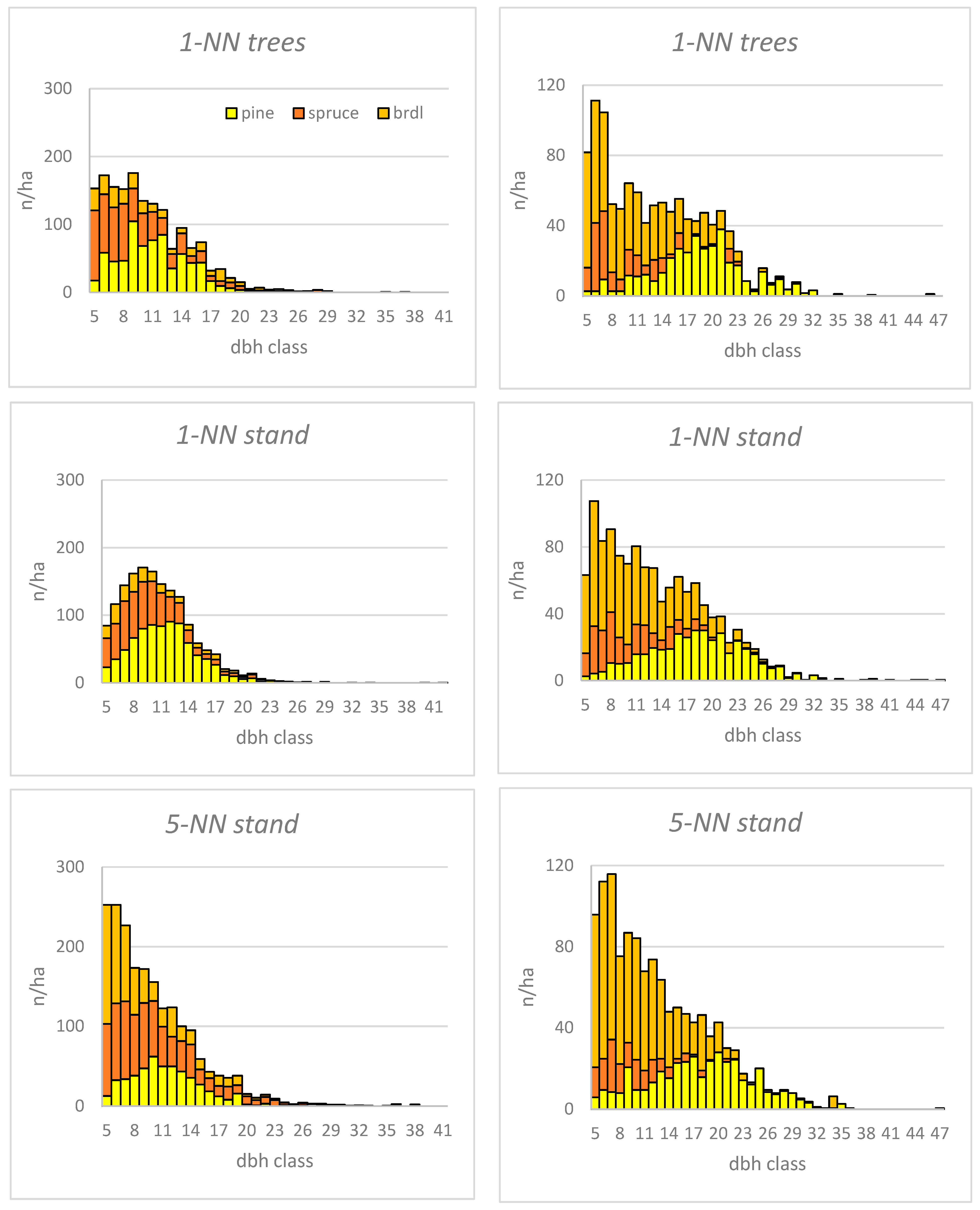
3.2. Differences in the Dbh Distributions between the Methods

In the k-NN_trees method, a stand was generated based on the measured trees of the NFI plots, whereas in the k-NN_stand method, a diameter distribution was generated based on the stand characteristics of the same plots. In practice, the same trees are used several times in the 1-NN_trees method when generating trees to the grid cells of a stand. This can be seen as peaks and hollows in the predicted dbh distribution for validation stands (Figure 2). In the model-based k-NN_stand method, the random selection of trees from the recovered Weibull distribution smooths the final dbh distribution (Figure 2). Despite this fundamental difference between 1-NN_trees and 1-NN_stand, these methods resulted in no major differences in the total stand volumes (Figure 3).

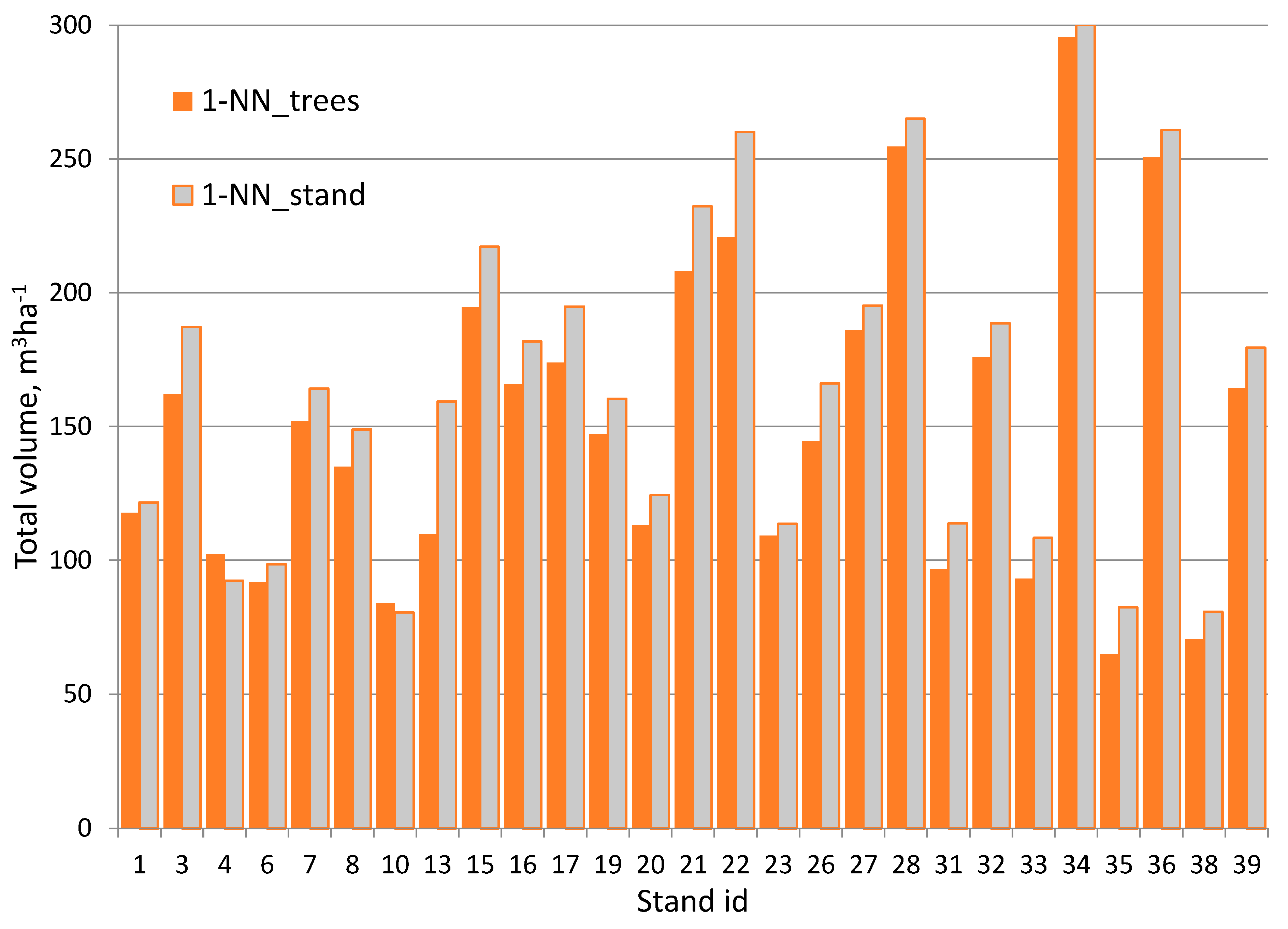
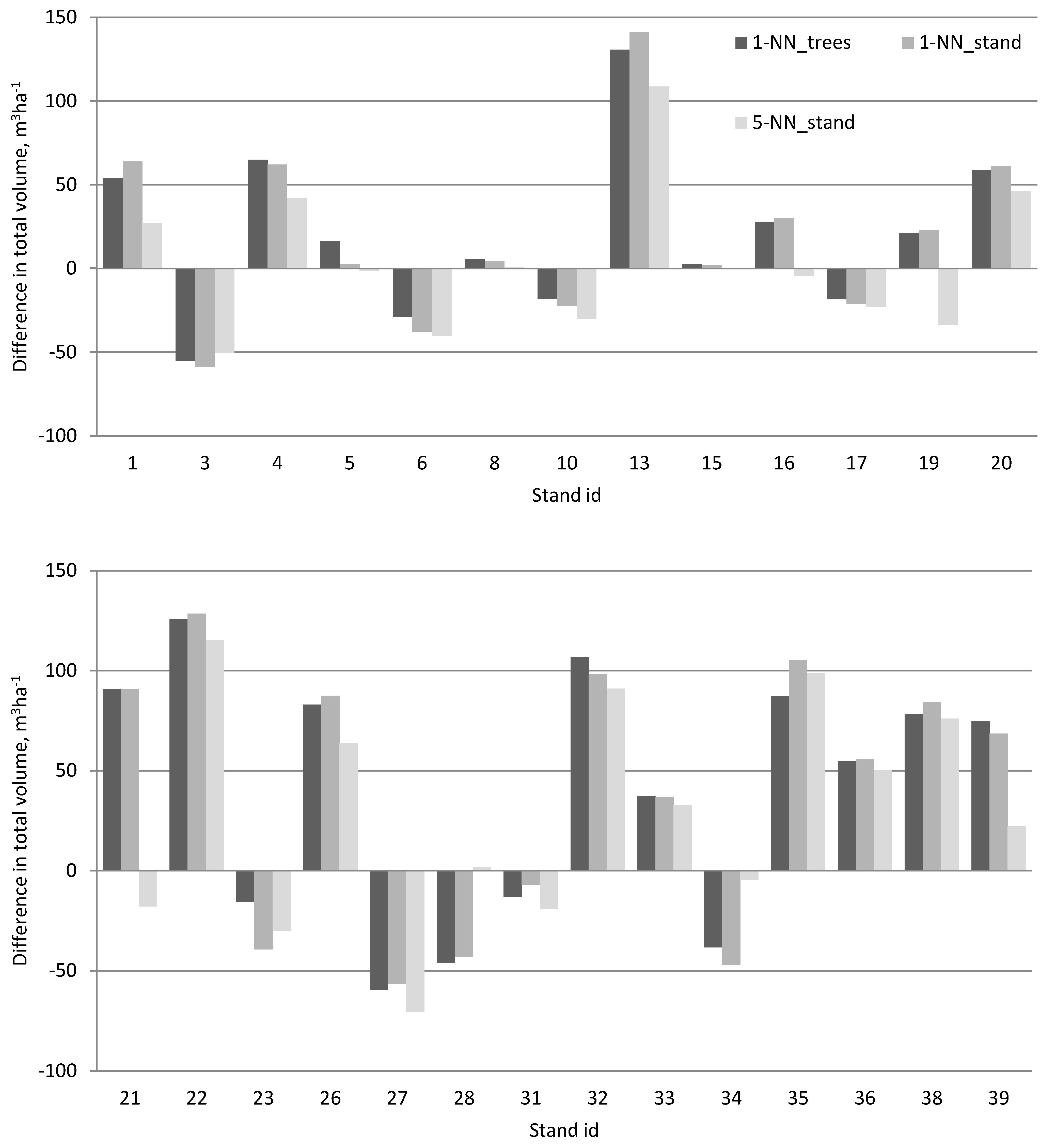
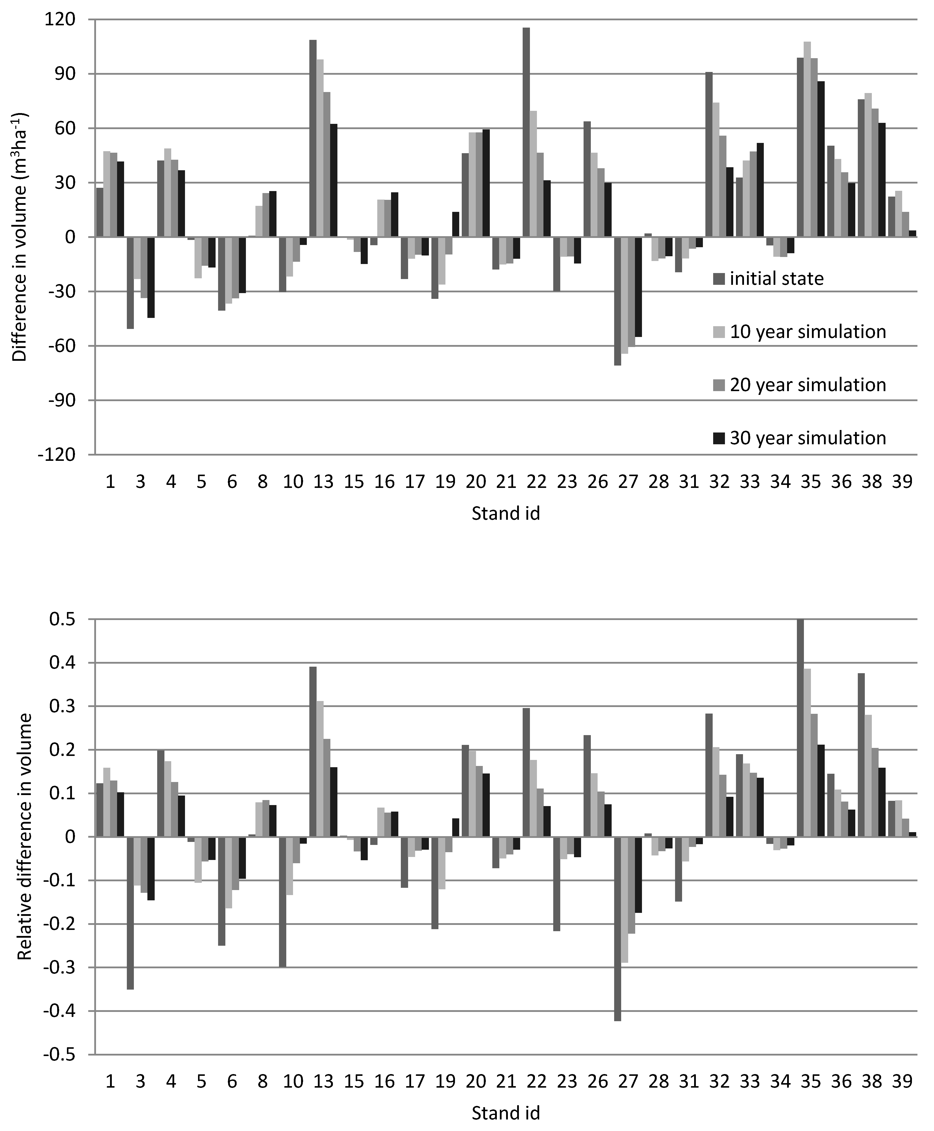
3.3. The Accuracy in the Initial Stand Volume and That after 30-Year Simulation

Regarding the ranking of the methods, the smallest difference (validation–prediction) in total stand volume (7.8%) to the validation data, as well as the smallest RMSE (24.7%), was given by the 5-NN_stand method (Table 4). The biggest difference in total volume (14.3%) was given by the 1-NN_trees method (Table 4). According to the RMSE in total and species-specific volumes, the 1-NN_stand was the worst method to generate the initial (updated to 2020 as in Figure 1) stand structure (Table 4). The relative RMSEs in the species-specific stem volumes were relatively high (61–69%), almost double the RMSE% for the whole stand (25–31%). Furthermore, one should note that the differences in the RMSE% between the species were only minor in the initial state.
All methods predicted higher stem volumes for pine compared with the validation data (Table 4). The largest difference by the 5-NN_stand method had an overestimation of 12.5 m3ha−1 (17%) and the smallest difference by the 1-NN_stand method amounted to a 10% difference in the initial state. In contrast, the methods estimated lower volumes for spruce and overall slightly lower volumes for broadleaved species compared to the validation data (Table 4). The largest difference in the spruce volume was found using the 1-NN_trees method by 34.2 m3ha−1 (37%). The smallest difference in the spruce volume (31%) was for the 5-NN_stand method. For the stem volume for broadleaved species, the 5-NN_stand method clearly provided a smaller difference (0.1 m3ha−1) to the observed volume than the other k-NN methods using k = 1 (Table 4). While the largest difference by the 1-NN_trees method amounted to 12.4%, the smallest difference in the 5-NN_stand method was only 0.1% in the initial state.
The differences between the observed and predicted total volumes for the different methods were often to the same direction in the individual stands, especially if the differences were high (Figure 4). The differences between the observed and predicted total volumes mostly became smaller with the higher k of 5 (19 cases had clear trend) while the result was vice versa for 4 cases only (stands 6, 10, 27, and 31).
After the 30-year simulation, the total volume was most similar to the simulation result based on the validation data for the 5-NN_stand method by underestimation of 8.5 m3ha−1 (2.3%) (Table 4). The highest mean difference 21.6 m3ha−1 (5.8%) was found using the 1-NN_trees method (Table 4). After the 30-year simulation, the initial differences between 17–31 m3ha−1 (8–14%) decreased to 9–22 m3ha−1 (2–6%) (Table 4).
The differences by tree species after a 30-year simulation were the most similar to the validation data for pine (2–6% difference) and broadleaves (6–9% difference), but the volume for spruce was still considerably underestimated (17–22%) (Table 4). The best performing methods varied only slightly depending on the considered characteristics. With the 5-NN_stand method, the volume for spruce was closest to that of the validation data. The 1-NN_stand method provided the least difference for pine and broadleaves. The smallest RMSE for tree species was always provided by the 5-NN_stand method. The 1-NN_stand method was the worst for RMSE for species-specific volumes similarly for the initial state and after the 30-year simulation (Table 4).
The order in the magnitude of prediction difference between the prediction methods was almost the same over time as for the initial state of stands (see Table 4). Yet, some changes could be found, e.g., the 5-NN_stand provided the smallest difference for broadleaves at the initial state while the 1-NN_stand methods provided the smallest difference after the 30-year simulation.
Along the simulation period, the relative differences between the prediction methods in the total volume decreased. As an example, the absolute and relative differences of the stand volume between the 5-NN_stand method and the volume of the validation data set over time are shown in Figure 5. A similar decrease occurred in most stands regardless of the prediction method, especially when the initial difference was large. In some stands when the difference in the predicted and measured initial state was small, the difference slightly increased over time (stands 8, 15, 16, 20 and 33, Figure 5). There was nothing in common for these stands (varying site types, including mineral soils and peatlands, planted or naturally regenerated, as well as thinned and unthinned stands). Similarly, there were no systematic differences among the stands for the highest initial differences except for the high initial overestimations, which were mostly on a dryish VT site.

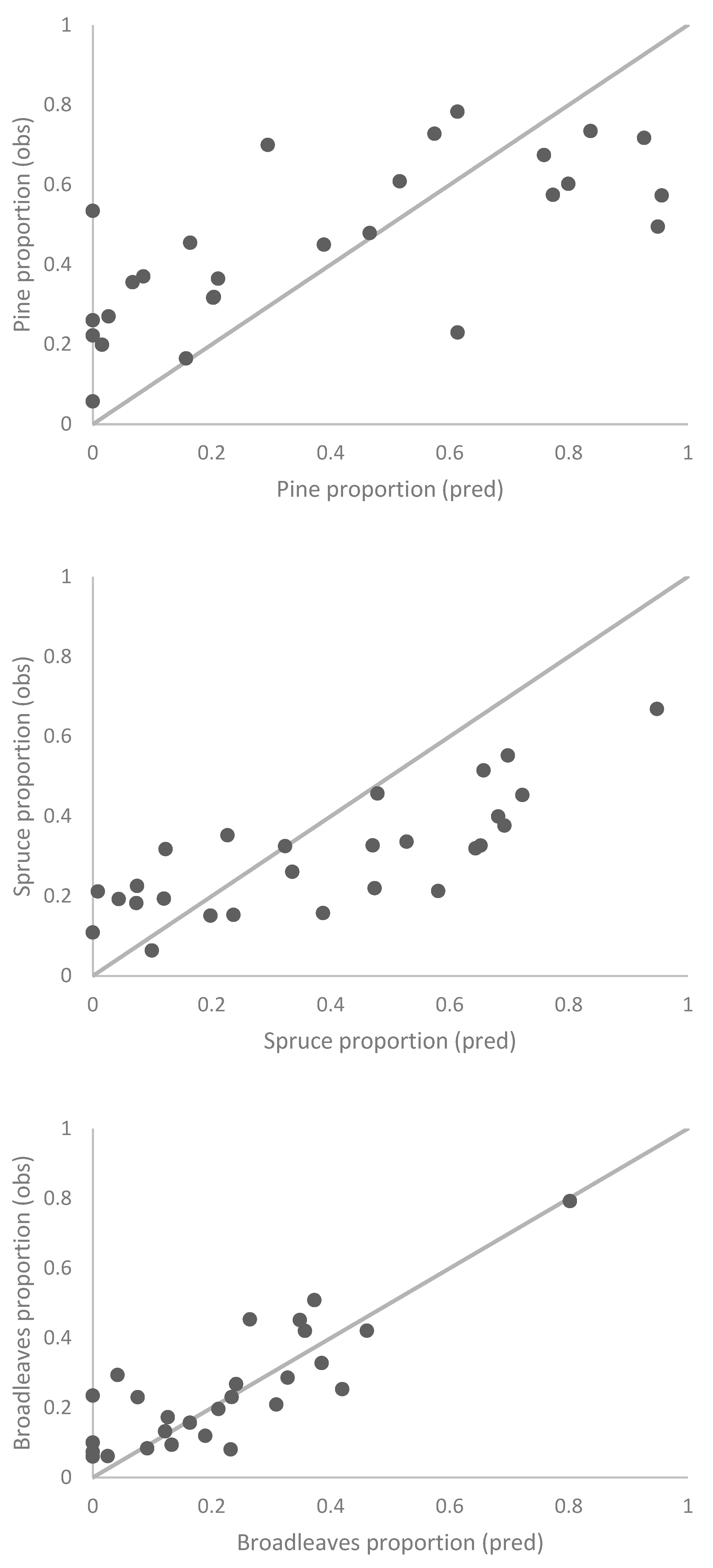
3.4. Species Proportion

The main tree species was defined from the proportion of initial volume by species. The main tree species was correctly predicted for 20 to 21 out of 27 cases (70–74% of cases). Thus, the difference between the best and worst result was only one case. The error matrix of the main tree species is shown for best results using the 5-NN_stand in Table 5. The error matrix showed that all the predicted seven spruce stands were spruce stands (Table 5). Also, the observed two broadleaved stands were predicted to be broadleaved dominated. However, four more stands were predicted to be broadleaved dominated and, thus, the prediction accuracy was only 33% (Table 5). The best accuracy for pine showed that 92% of the observed pine stands were predicted to be pine stand and 79% of the predicted pine stands were pine dominated (Table 3).
As an example, Figure 6 shows the species proportion in the validation data and in the best performed 5-NN_stand prediction method. Regardless of the value of k in the k-NN prediction method, the proportion of tree species resembled that of the example with the 5-NN_stand method in Figure 6. Generally, the prediction methods provided smaller spruce proportions for the spruce-dominated stands compared with the validation data. For stand no. 13, the observed data did not include pine but the predicted proportion of pine was as high as 53%.

4. Discussion

This study evaluated the potential of MS-NFI pixel-level data for the generation of individual stand tree lists and compared alternative prediction methods for diameter distribution. The advantage of using satellite-based data instead of ALS is the lower costs and generally up-to-date availability. At first, we evaluated the effect of k in k-NN method on the accuracy of plot-level stand characteristics, DG, G and N. Increasing k decreased the level of error in most of the evaluated variables in the plot-level preliminary study. On the other hand, almost each value of k (1, 3, 4, 5), except k = 2, performed the best for at least one validated characteristic. Similarly, in other previous studies, when varying k (3–6), each of them provided the best results for some stand characteristics while the generally best results were given by k = 4 [44] or k = 5 [47]. Nevertheless, we did not find one single best value for k and ended up selecting k values 1 and 5 for the stand-level study. Value 1 was justified because of reasonable accuracy and as a base method, which retains the original plot-level variance [42,48]. On the other hand, value 5 provided the most accurate G which is highly correlated with stand volume. According to a review by Chirici et al. [33], the most frequently applied values of k were 1, 5 and 10. When k was optimized, the solution was frequently 4, 5 or 6 depending on neighbor weighting and number of feature variables [49]. The validation plot-level RMSE in G in our study varied between 33% and 43% depending on k and in DG the variation was 26–27%. Note that Tomppo et al. [36] using ALS-assisted estimates (aerial photographs for species detection) reported higher accuracy, namely the corresponding RMSE of 22% in G and 11% in D for the same plots.
Our stand-level validation data consisted of 15 photos per stand using the Trestima smart-phone app and inventory method [34]. No published results exist on the accuracy of the Trestima approach in identifying the smallest trees of a stand. Vastaranta et al. [50] studied the Trestima approach for sample plot measurements (basal area, mean diameter, mean height), but unfortunately the accuracy in stem number was not included. According to Siipilehto et al. [42] and Ruusunen [51], the bias in the stem number was between 2% and 5%, while the RMSE% was between 32% and 34% when using the Trestima approach. According to Dunaeva [52], the stem number estimates by the Trestima approach were more accurate than the estimates by forest experts in a preharvest field inventory. Also, the tree species composition was accurately estimated by Trestima compared to the harvester-based validation data [52].
In general, the MS-NFI based methods (k-NN_trees, k-NN_stand) performed well for the total stand volume, and the average difference between the predicted and validation volumes ranged from 8% to 14%. The RMSE% using the satellite-based MS-NFI data varied between 25–31%, which was much smaller than in previous studies using Landsat imagery. Indeed, e.g., Mäkelä and Pekkarinen [53] reported considerably larger 48% RMSE in total volume at stand-level using Landsat imagery. However, in Mäkelä and Pekkarinen [53], the standwise results were predicted directly whereas in our study the standwise results were computed from predictions for pixels in the stand. In addition, the data in Mäkelä and Pekkarinen [53] included all kinds of stands from the planning area. Other previous studies have also reported RMSE% from 42% to 50% for total volume using satellite-based data for stand-level volume [54,55,56]. It is therefore possible that the improved accuracy in satellite imagery is the reason for the improved accuracy in stand volume. According to Astola et al. [57], Sentinel 2 MSI outperformed Landsat 8 OLI when predicting stand total and species-wise characteristics. In Germany, Nink et al. [58] reported an RMSE% of 21.6 for stand-level Norway spruce timber volume using k-NN and Sentinel 2. Further improvement in the accuracy of prediction could have been gained in this study using other advanced machine learning methods, such as Random Forests [59]. However, there is a long time-series of MS-NFI thematic maps produced employing the (improved) k-NN estimation [3], which justifies the use of the same method.
In addition to the number and size of trees, information on tree species composition is a key parameter describing the stand structure for a wide variety of applications in forest management and conservation. The classification of stands by tree species composition is a complex task using satellite- or ALS-based data [60,61], and the results of the present study were considered satisfactory. In this study, spruce was the most abundant tree species, pine was slightly less frequent and broadleaves clearly a minority species. The main tree species was satisfactorily predicted, and the species proportions were generally quite well estimated, especially for broadleaves. However, the predicted stand-level tree lists always included pine, spruce and broadleaved species, even if one of them did not exist in the Trestima validation data. Relatively good results for tree species dominance using Landsat TM and Sentinel-2 with NFI plots have been reported by Tomppo et al. [62], Persson et al. [63] and Breidenbach et al. [64], especially for conifer species.
The validation data in the present study was rather small (27 stands) and the differences in the total and species-specific volume estimates were larger than in previous studies based on ALS (e.g., [65,66]). Indeed, the average differences in total volume were 13% for Scots pine and 35% for Norway spruce. Nevertheless, the stem volume for broadleaves in this study was at its best almost unbiased (0.1–1%) and otherwise at the same level (7–16%) to that by Packalén and Maltamo [67], namely a bias of 11%. It is presumable that the smaller number of stands and different methods (satellite imagery vs. ALS) are the main reasons for the relatively high bias in this study. In addition, the stands of the present study were selected from stands with an irregular stand structure, in which an estimation with remote sensing methods usually leads to large RMSEs. However, it should be noted that low-volume stands were absent from the validation data, which may result in a reduction in the RMSEs. Using k-NN and Sentinel-2 data, Nink et al. [58] found only 1.3% bias in timber volume for the selected 56 pure Norway spruce stands which had mean timber volume of 284 m3ha−1.
Maltamo et al. [65] and Tomppo et al. [36] reported increased accuracy in stand characteristics using fixed area instead of relascope plots as training data. Note that only the latest fixed area NFI plots were applied in this study. Also, one reason for the relatively similar results with the prediction methods was the update of the data set from 2015 to inventory year 2020. Even if the update period was short, updating has an averaging feature. For example, Figure 5 shows how much the first simulated 10-year period decreased the initial differences in stand volume.
When Holopainen et al. [68] studied uncertainty in timber assortment estimates predicted from forest inventory data, the main source of error was forest inventory, either stand-wise field inventory or ALS-based inventory, while the effects of generated stem distribution errors were minor. In Finland, when the stand-wise management-oriented field inventory was changed to the ALS-based inventory, the mean stand characteristics were also changed from basal area-median tree dimensions (DGM, HGM) to weighted means (DG, HG). Recent results showed that DG is more stable in parameter recovery than DGM [69]. Thus, the parameter recovery method makes the distribution errors negligible.
Räty [27] states that there is a forthcoming shift in practical forest management planning from distribution models to k-NN-based tree lists. It is also worth noting that the increase in the value of k also considerably increased the required computational capacity and simulation time for k-NN_tree methods. The present study found it impossible to simulate five times (k = 5) the number of trees (N) when generating a dbh distribution: when k was 5, the number of trees of about 35,600 for a stand compartment was too much for a Motti simulator. The practical solution was to use only the 5-NN_stand method when k was 5 and generate only N/k trees from each k-recovered Weibull distribution. By doing so, the number of trees in the simulation was restricted to the number of trees per hectare multiplied with the area of the stand compartment. In the case of the present study, the maximum number of simulated trees using the k-NN_stand method was 6780 trees for a 6.5 ha stand compartment.
Finally, each k species-specific stand characteristic was used for the parameter recovery and thus this successfully mimicked the realization of measured trees. Previously, Maltamo and Kangas [4] found clearly better results with the k-NN empirical distribution (i.e., k-NN_trees) compared with the prediction of the Weibull function. However, the applied prediction model for the Weibull distribution [70] was not as flexible as the parameter recovery method used in this study [29]. Subsequently, Packalén and Maltamo [10] achieved slightly better results using 5-MSN empirical distribution in comparison to calibrated Weibull distributions derived from ALS-based stand characteristics. Similarly, in our study, the 1-NN_trees method demonstrated a slight advantage over the 1-NN_stand method. Nevertheless, the 5-NN_stand method consistently yielded superior results in comparison to the 1-NN_trees or 1-NN_stand methods, with the exception of two instances.
The stand development was simulated over time and the effects of biases were compared in the initial stand structure by the different prediction methods. The 30-year simulation showed that differences between the prediction methods occur as long as the initial state has some influence on stand development, though selecting the prediction method for the initial stand became less significant over time. Even though the rank between the methods did not change much over time, the differences between the methods decreased. Similar results have been reported previously [71,72,73], with the reason most likely due to the feature that individual tree models predict higher diameter growth and less mortality for stands in which stocking levels were initially underestimated and vice versa. If the initial state was accurate, the differences could even increase during simulation. Accordingly, Kangas and Maltamo [71] noticed that a calibrated, more accurate initial state did not improve the accuracy of the predicted future volumes after simulation. The simulations of this study were carried out without intermediate disturbances, e.g., thinnings or damage, which would further reduce the effect of the predicted initial state on stand development. Thus, the selection of the prediction method can be made according to convenience to handle the data.

5. Conclusions

The MS-NFI pixel-level data proved feasible for generating tree lists of individual stands. The advantage of using satellite-based data instead of ALS is that it is freely accessible and up-to-date. Moreover, alternative methods to produce tree lists for describing the stands resulted in no major differences in the stand volumes and they predicted the main tree species of the stands accurately. However, according to the results of the stand characteristics analysis, the 5-NN_stand method can be recommended. For forest management purposes, the target accuracy for basal area, mean diameter and total volume is 20% in stand-level for an ALS-based inventory method in Finland. Even if the accuracy improved much from earlier studies using satellite-based data, the accuracy can be considered slightly too low for management purposes. In addition, the volume estimates by species were less accurate, which calls for further development in distinction between tree species in the MS-NFI data. As the effects of the initial stand characteristics decreased over time, the choice of the method when generating input data for a long-term simulation appeared to be less influential.

Author Contributions

Data acquisition and processing: J.S., M.K. and H.M.H.; project administration: H.M. All authors have read and agreed to the published version of the manuscript.

Funding

This study was financially supported by the Research Council of Finland (grant no 315495).

Data Availability Statement

Landsat 8 OLI and Sentinel 2 MSI images are open access data; NFI field data are available for research purposes on request. The data used and code are available on request from the corresponding author.

Acknowledgments

We would like to express our gratitude to Lic. Tech. Kai Mäkisara for processing the MS-NFI data and for providing valuable comments on the manuscript. We would also like to thank the field staff of Luke, in particular Jukka Lehtimäki, for their assistance.

Conflicts of Interest

The authors declare no conflicts of interest.

References

  1. Tomppo, E. Satellite image-based National Forest Inventory of Finland. Photogramm. J. Finl. 1990, 12, 115–120. [Google Scholar]
  2. Tomppo, E.; Haakana, M.; Katila, M.; Peräsaari, J. Multi-Source National Forest Inventory: Methods and Applications; Springer Science & Business Media: Dodrecht, The Netherlands, 2008. [Google Scholar]
  3. Mäkisara, K.; Katila, M.; Peräsaari, J. The Multi-Source National Forest Inventory of Finland—Methods and Results 2015. Natural Resources and Bioeconomy Studies 8/2019, Natural Resources Institute Finland. 2019. 57p. Available online: https://urn.fi/URN:ISBN:978-952-326-711-4 (accessed on 1 July 2024).
  4. Maltamo, M.; Kangas, A. Methods based on k-nearest neighbor regression in the prediction of basal area diameter distribution. Can. J. For. Res. 1998, 28, 1107–1115. [Google Scholar] [CrossRef]
  5. Næsset, E. Estimating timber volume of forest stands using airborne laser scanner data. Remote Sens. Environ. 1997, 61, 246–253. [Google Scholar] [CrossRef]
  6. Næsset, E. Predicting forest stand characteristics with airborne scanning laser using a practical two-stage procedure and field data. Remote Sens. Environ. 2002, 80, 88–99. [Google Scholar] [CrossRef]
  7. Næsset, E. Practical large-scale forest stand inventory using a small-footprint airborne laser scanning. Scand. J. For. Res. 2004, 19, 164–179. [Google Scholar] [CrossRef]
  8. Kangas, A.; Astrup, R.; Breidenbach, J.; Fridman, J.; Gobakken, T.; Korhonen, K.T.; Maltamo, M.; Nilsson, M.; Nord-larsen, T.; Næsset, E.; et al. Remote Sensing and Forest Inventories in Nordic Countries—Roadmap for the Future. Scand. J. For. Res. 2018, 33, 397–412. [Google Scholar] [CrossRef]
  9. Holmgren, P.; Thuresson, T. Satellite remote sensing for forestry planning—A review. Scand. J. For. Res. 1998, 13, 90–110. [Google Scholar] [CrossRef]
  10. Packalén, P.; Maltamo, M. Estimation of species-specific diameter distributions using airborne laser scanning and aerial photographs. Can. J. For. Res. 2008, 38, 1750–1760. [Google Scholar] [CrossRef]
  11. Peuhkurinen, J.; Maltamo, M.; Malinen, J. Estimating species-specific diameter distributions and saw log recoveries of boreal forests from airborne laser scanning data and aerial photographs: A distribution-based approach. Silva Fenn. 2008, 42, 625–641. [Google Scholar] [CrossRef]
  12. Barrett, F.; McRoberts, R.E.; Tomppo, E.; Cienciala, E.; Waser, L.T. A questionnaire-based review of the operational use of remotely sensed data by national forest inventories. Remote Sens. Environ. 2016, 174, 279–289. [Google Scholar] [CrossRef]
  13. Nilsson, M. Estimation of Forest Variables Using Satellite Image Data and Airborne Lidar. Ph.D. Thesis, Swedish University of Agricultural Sciences, The Department of Forest Resource Management and Geomatics, Acta Universitas Agriculture Sueciae, Uppsala, Sweden, 1997; 84p. [Google Scholar]
  14. Næsset, E.; Gobakken, T.; Holmgren, J.; Hyyppä, H.; Hyyppä, J.; Maltamo, M.; Nilsson, M.; Olsson, H.; Persson, Å.; Söderman, U. Laser scanning of forest resources: The Nordic experience. Scand. J. For. Res. 2004, 19, 482–499. [Google Scholar] [CrossRef]
  15. Maltamo, M.; Packalén, P.; Peuhkurinen, J.; Suvanto, A.; Pesonen, A.; Hyyppä, J. Experiences and possibilities of ALS based forest inventory in Finland. In Proceedings of the ISPRS Workshop on Laser Scanning 2007 and SilviLaser 2007, Espoo, Finland, 12–14 September 2007; pp. 270–279. [Google Scholar]
  16. McRoberts, R.E.; Cohen, W.B.; Næsset, E.; Stehman, S.V.; Tomppo, E.O. Using remotely sensed data to construct and assess forest attribute maps and related spatial products. Scand. J. For. Res. 2010, 25, 340–367. [Google Scholar] [CrossRef]
  17. Maltamo, M.; Packalen, P. Species-Specific Management Inventory in Finland. In Forestry Applications of Airborne Laser Scanning. Managing Forest Ecosystems; Maltamo, M., Næsset, E., Vauhkonen, J., Eds.; Springer: Dordrecht, The Netherlands, 2014; Volume 27. [Google Scholar] [CrossRef]
  18. Fassnacht, F.E.; White, J.C.; Wulder, M.A.; Næsset, E. Remote sensing in forestry: Current challenges, considerations and directions. Forestry 2024, 97, 11–37. [Google Scholar] [CrossRef]
  19. Wulder, M.A.; Hermosilla, T.; White, J.C.; Bater, C.W.; Hobart, G.; Bronson, S.C. Development and implementation of a stand-level satellite-based forest inventory for Canada. Forestry 2024, 1, cpad065. [Google Scholar] [CrossRef]
  20. Zhang, J.; Foody, G.M. A fuzzy classification of sub-urban land cover from remotely sensed imagery. Int. J. Remote Sens. 1998, 19, 2721–2738. [Google Scholar] [CrossRef]
  21. Wikström, P. Effect of decision variable definition and data aggregation on search process applied to a single-tree simulator. Can. J. For. Res. 2001, 31, 1057–1066. [Google Scholar] [CrossRef]
  22. Ahtikoski, A.; Siipilehto, J.; Salminen, H.; Lehtonen, M.; Hynynen, J. Effect of stand structure and number of sample trees on optimal management for Scots pine: A model-based study. Forests 2018, 9, 750. [Google Scholar] [CrossRef]
  23. Maltamo, M. Basal Area Diameter Distribution in Estimating the Quantity and Structure of Growing Stock. Doctoral Dissertation, University of Joensuu, Faculty of Forestry, Joensuu, Finland, 1998. [Google Scholar]
  24. Mehtätalo, L. Predicting Stand Characteristics Using Limited Measurements. Finnish Forest Research Institute, Research Papers 929. 2004. 39p. Available online: http://urn.fi/URN:ISBN:951-40-1934-2 (accessed on 1 July 2024).
  25. Packalén, P. Using airborne laser scanning data and digital aerial photographs to estimate growing stock by tree species. Diss. For. 2009, 77, 41. [Google Scholar] [CrossRef]
  26. Siipilehto, J. Methods and applications for improving parameter prediction models for stand structures in Finland. Diss. For. 2011, 124, 56. [Google Scholar] [CrossRef]
  27. Räty, J. Prediction of diameter distributions in boreal forests using remotely sensed data. Diss. For. 2020, 294, 47. [Google Scholar] [CrossRef]
  28. Bailey, R.L.; Dell, T.R. Quantifying diameter distributions with the Weibull function. For. Sci. 1973, 19, 97–104. [Google Scholar]
  29. Siipilehto, J.; Mehtätalo, L. Parameter recovery vs. parameter prediction for the Weibull distribution validated for Scots pine stands in Finland. Silva Fenn. 2013, 47, 1–22. [Google Scholar] [CrossRef]
  30. Moeur, M.; Stage, A.R. Most similar neighbor: An improved sampling inference procedure for natural resource planning. For. Sci. 1995, 41, 337–359. [Google Scholar] [CrossRef]
  31. Maltamo, M.; Malinen, J.; Kangas, A.; Härkönen, S.; Pasanen, A.-M. Most similar neighbor-based stand variable estimation for use in inventory by compartments in Finland. Forestry 2003, 76, 449–463. [Google Scholar] [CrossRef]
  32. Fix, E.; Hodges, J.L. Discriminatory Analysis: Nonparametric Discrimination: Consistency Properties; USAF School of Aviation Medicine: Randolf Field, TX, USA, 1951. [Google Scholar]
  33. Chirici, G.; Mura, M.; McInerney, D.; Py, N.; Tomppo, E.; Waser, L.T.; Travaglini, D.; McRoberts, R.E. A meta-analysis and review of the literature on the k-nearest neighbors technique for forestry applications that use remotely sensed data. Remote Sens. Environ. 2016, 176, 282–294. [Google Scholar] [CrossRef]
  34. Rouvinen, T. Kuvia metsästä. [Photos from forest]. Metsätieteen Aikakauskirja 2014, 2, 119–122. [Google Scholar] [CrossRef]
  35. Trestima. Forest Inventory System. User Manual v.1.4. 2020. Available online: https://www.trestima.com/w/wp-content/uploads/2020/02/TRESTIMA_user_guide_en_v1.4.pdf (accessed on 1 July 2024).
  36. Tomppo, E.; Kuusinen, N.; Mäkisara, K.; Katila, M.; McRoberts, R.E. Effect of field plot configuration on the uncertainties of ALS-assisted forest resource estimates. Scand. J. For. Res. 2017, 32, 488–500. [Google Scholar] [CrossRef]
  37. Cajander, A.K. Forest types and their significance. Acta For. Fenn. 1949, 56, 1–69. [Google Scholar] [CrossRef]
  38. Salminen, H.; Lehtonen, M.; Hynynen, J. Reusing legacy FORTRAN in MOTTI growth and yield simulator. Comput. Electron. Agr. 2005, 49, 105–113. [Google Scholar] [CrossRef]
  39. Hynynen, J.; Salminen, H.; Ahtikoski, A.; Huuskonen, S.; Ojansuu, R.; Siipilehto, J.; Lehtonen, M.; Eerikäinen, K. Long-term impacts of forest management on biomass supply and forest resource development: A scenario analysis for Finland. Eur. J. For. Res. 2015, 134, 415–431. [Google Scholar] [CrossRef]
  40. Rogers, W.H. Some Convergence Properties of k-Nearest Neighbor Estimates; Department of Statistics, Stanford University: Palo Alto, CA, USA, 1978. [Google Scholar]
  41. Tomppo, E.; Halme, M. Using coarse scale forest variables as ancillary information and weighting of variables in k-NN estimation: A genetic algorithm approach. Remote Sens. Environ. 2004, 92, 1–20. [Google Scholar] [CrossRef]
  42. Siipilehto, J.; Lindeman, H.; Vastaranta, M.; Yu, X.; Uusitalo, J. Reliability of the predicted stand structure for clear-cut stands using optional methods: Airborne laser scanning-based methods, smartphone-based forest inventory application Trestima and pre-harvest measurement tool EMO. Silva Fenn. 2016, 50, 1568. [Google Scholar] [CrossRef]
  43. Geman, S.; Bienenstock, E.; Doursat, R. Neural networks and the bias/variance dilemma. Neural Comput. 1992, 4, 1–58. [Google Scholar] [CrossRef]
  44. Holopainen, M.; Tuominen, S.; Karjalainen, M.; Hyyppä, J.; Vastaranta, M.; Hyyppä, H. Korkearesoluutioisten E-SAR-tutkakuvien tarkkuus puustotunnusten koealatason estimoinnissa. Metsätieteen Aikakauskirja 2009, 4, 309–323. [Google Scholar] [CrossRef]
  45. Siipilehto, J.; Kangas, A. Näslundin pituuskäyrä ja siihen perustuvia malleja läpimitta-pituus riippuvuudesta suomalaisissa talousmetsissä. [Näslund’s hight curve models for the dbh-height relationship in Finnish commercial forests.]. Metsätieteen Aikakauskirja 2015, 4, 215–236. [Google Scholar] [CrossRef]
  46. Laasasenaho, J. Taper curve and volume functions for pine, spruce and birch. Commun. Inst. For. Fenn. 1982, 108, 1–74. [Google Scholar]
  47. Tuominen, S.; Balazs, A.; Honkavaara, E.; Pölönen, I.; Saari, H.; Hakala, T.; Viljanen, N. Hyperspectral UAV-imagery and photogrammetric canopy height model in estimating forest stand variables. Silva Fenn. 2017, 51, 7721. [Google Scholar] [CrossRef]
  48. Hudak, A.T.; Crookston, N.L.; Evans, J.S.; Hall, D.E.; Falkowski, M.J. Nearest neighbor imputation of species-level, plot-scale forest structure attributes from LiDAR data. Remote Sens. Environ. 2008, 112, 2232–2245. [Google Scholar] [CrossRef]
  49. McRoberts, R.E.; Næsset, E.; Gobakken, T. Optimizing the k-Nearest Neighbors technique for estimating forest aboveground biomass using airborne laser scanning data. Remote Sens. Environ. 2015, 163, 13–22. [Google Scholar] [CrossRef]
  50. Vastaranta, M.; Gonzalez Latorre, E.; Luoma, V.; Saarinen, N.; Holopainen, M.; Hyyppä, J. Evaluation of a smartphone app for forest sample plot measurements. Forests 2015, 6, 1179–1194. [Google Scholar] [CrossRef]
  51. Ruusunen, P. Trestiman Puustotulkinnan Tarkkuus Tarkkaan Mitatuilla Puukarttakoealoilla. [Trestima’s Accuracy in Accurately Measured Tree Map Plots]. Häme University of Applied Sciences. 2020. 41p. Available online: https://urn.fi/URN:NBN:fi:amk-202004165202 (accessed on 1 July 2024).
  52. Dunaeva, T. Preharvest Efficiency of Trestima, Airborne Laser Scanning and Forest Management Plan Data Validated by Actual harvesting Results and Forest Engineer Preharvest Estimation. Bachelor’s Thesis, Yrkehögskolan NOVIA, Raseborg, Finland, 2017; 98p. [Google Scholar]
  53. Mäkelä, H.; Pekkarinen, A. Estimation of forest stand volumes by Landsat TM imagery and stand-level field-inventory data. For. Ecol. Manag 2004, 196, 245–255. [Google Scholar] [CrossRef]
  54. Hyyppä, J.; Hyyppä, H.; Inkinen, M.; Engdahl, M.; Linko, S.; Zhu, Y.-H. Accuracy comparison of various remote sensing data sources in the retrieval of forest stand attributes. For. Ecol. Manag. 2000, 128, 109–120. [Google Scholar] [CrossRef]
  55. Hyvönen, P. Kuvioittaisten puustotunnusten ja toimenpide-ehdotusten estimointi k-lähimmän naapurin menetelmällä Landsat TM -satelliittikuvan, vanhan inventointitiedon ja kuviotason tukiaineiston avulla. Metsätieteen Aikakauskirja 2002, 3, 363–379. (In Finnish) [Google Scholar] [CrossRef]
  56. Muukkonen, P.; Heiskanen, J. Estimating biomass for boreal forests using ASTER satellite data combined with standwise forest inventory data. Remote Sens. Environ. 2005, 99, 434–447. [Google Scholar] [CrossRef]
  57. Astola, H.; Häme, T.; Sirro, L.; Molinier, M.; Kilpi, J. Comparison of Sentinel-2 and Landsat 8 imagery for forest variable prediction in boreal region. Remote Sens. Environ. 2019, 223, 257–273. [Google Scholar] [CrossRef]
  58. Nink, S.; Hill, J.; Buddenbaum, H.; Stoffels, J.; Sachtleber, T.; Langshausen, J. Assessing the Suitability of Future Multi- and Hyperspectral Satellite Systems for Mapping the Spatial Distribution of Norway Spruce Timber Volume. Remote Sens. 2015, 7, 12009–12040. [Google Scholar] [CrossRef]
  59. Esteban, J.; McRoberts, R.E.; Fernández-Landa, A.; Tomé, J.L.; Næsset, E. Estimating Forest Volume and Biomass and Their Changes Using Random Forests and Remotely Sensed Data. Remote Sens. 2019, 11, 1944. [Google Scholar] [CrossRef]
  60. Holopainen, M.; Haapanen, R.; Tuominen, S.; Viitala, R. Performance of airborne laser scanning- and aerial photograph-based statistical and textural features in forest variable estimation. In Proceedings of the SilviLaser, Edinburgh, UK, 17–19 September 2008. [Google Scholar]
  61. Hovi, A.; Raitio, P.; Rautiainen, M. A spectral analysis of 25 boreal tree species. Silva Fenn. 2017, 51, 7753. [Google Scholar] [CrossRef]
  62. Tomppo, E.; Gagliano, C.; De Natale, F.; Katila, M.; McRoberts, R.E. Predicting categorical forest variables using an improved k-Nearest Neighbour estimator and Landsat imagery. Remote Sens. Environ. 2009, 113, 500–517. [Google Scholar] [CrossRef]
  63. Persson, M.; Lindberg, E.; Reese, H. Tree classification with Multi-Temporal Sentinel-2 data. Remote Sens. 2018, 10, 1794. [Google Scholar] [CrossRef]
  64. Breidenbach, J.; Waser, L.T.; Debella-Gilo, M.; Schumacher, J.; Rahlf, J.; Hauglin, M.; Puliti, S.; Astrup, R. National mapping and estimation of forest area by dominant tree species using Sentinel-2 data. Can. J. For. Res. 2020, 51, 365–379. [Google Scholar] [CrossRef]
  65. Maltamo, M.; Packalén, P.; Suvanto, A.; Korhonen, K.T.; Mehtätalo, L.; Hyvönen, P. Combining ALS and NFI training data for forest management planning: A case study in Kuortane, Western Finland. Eur. J. For. Res. 2009, 128, 305–317. [Google Scholar] [CrossRef]
  66. Tuominen, S.; Pitkänen, J.; Balazs, A.; Korhonen, K.T.; Hyvönen, P.; Muinonen, E. NFI plots as complementary reference data in forest inventory based on airborne laser scanning and aerial photography in Finland. Silva Fenn. 2014, 48, 983. [Google Scholar] [CrossRef]
  67. Packalén, P.; Maltamo, M. The k-MSN method for the prediction of species-specific stand attributes using airborne laser scanning and aerial photographs. Remote Sens. Environ. 2007, 109, 328–341. [Google Scholar] [CrossRef]
  68. Holopainen, M.; Vastaranta, M.; Rasinmäki, J.; Kalliovirta, J.; Mäkinen, A.; Haapanen, R.; Melkas, T.; Yu, X.; Hyyppä, J. Uncertainty in timber assortment estimates predicted from forest inventory data. Eur. J. For. Res. 2010, 129, 1131–1142. [Google Scholar] [CrossRef]
  69. Lee, D.; Siipilehto, J.; Hynynen, J. Models for diameter distribution and tree height in hybrid aspen plantations in southern Finland. Silva Fenn. 2021, 55, 10612. [Google Scholar] [CrossRef]
  70. Maltamo, M. Comparing basal area diameter distributions estimated by tree species and for the entire growing stock in a mixed stand. Silva Fenn. 1997, 31, 53–65. [Google Scholar] [CrossRef]
  71. Siipilehto, J. Improving the accuracy of predicted basal-area diameter distribution in advanced stands by determining stem number. Silva Fenn. 1999, 33, 281–301. [Google Scholar] [CrossRef]
  72. Kangas, A.; Maltamo, M. Calibrating predicted diameter distribution with additional information in growth and yield predictions. Can. J. For. Res. 2003, 33, 430–434. [Google Scholar] [CrossRef]
  73. Mäkinen, A.; Holopainen, M.; Kangas, A.; Rasinmäki, J. Propagating the errors of initial forest variables through stand- and tree-level growth simulators. Eur. J. For. Res. 2010, 129, 887–897. [Google Scholar] [CrossRef]
Figure 1. The general workflow for predicting individual trees of a stand (diameter, height, volume) in the alternative Nearest Neighbor (NN) prediction methods using Multi-Source National Forest Inventory (NFI) data to compare their predictions with the plot- and stand-level validation data sets.
Remotesensing 16 02513 g001
Figure 2. Example of the predicted species-specific dbh distributions using the alternative methods for validation stands no. 2 (left) and 11 (right). In the k-Nearest Neigbor (k-NN) method name, trees means that distribution is generated directly from the measured trees of the selected NFI field plot whereas stand means that stand characteristics of these plots are used for recovering Weibull distribution and sampling the tree diameters randomly.
Remotesensing 16 02513 g002
Figure 3. The total volume (m3ha−1) of the validation stands using methods 1-NN_trees (selecting measured trees from the NFI sample plots) and 1-NN_stand (trees were randomly sampled from the predicted grid-level species-specific distributions of the same NFI plots).
Remotesensing 16 02513 g003
Figure 4. Differences in the stand-level total volume per hectare between the prediction methods and the validation data (observed–predicted).
Remotesensing 16 02513 g004
Figure 5. The absolute and relative difference (RD, Equation (2)) in the stand volume over time between the 5-NN_stand method and validation data at the initial state (updated to 2020) and after 10, 20 and 30-year simulation ([5-NN_stand—validation]/validation]).
Remotesensing 16 02513 g005
Figure 6. Proportion of tree species of the total stand volume according to the observed validation data (y-axis) and the 5-NN_stand predictions (x-axis).
Remotesensing 16 02513 g006
Table 1. The characteristics of the validation data (27 stands measured in 2020) and plot-level characteristics (32 m × 32 m plots in the same stands, measured in 2014).
VariableMeanStdevMinMax
Plot-level characteristics (in 2014)
Basal area, m2ha−123.18.59.142.0
Stem number, ha−122001006430.4619
DG * (all species), cm15.15.67.728.9
Stand-level characteristics (in 2020)
Age, years46.722.619110
Dominant height, m18.53.212.725.2
Basal area, m2ha−126.67.616.245
Stem number, ha−112796234392348
DG * (all species), cm20.84.813.730
Total stem volume (V), m3ha−1213.672.7101.4390.5
V * for Scots pine, m3ha−174.864.00.0209.5
V for Norway spruce, m3ha−193.079.60.0278.9
V for broadleaves, m3ha−145.735.70.0116.7
* DG is basal-area-weighted mean tree stem diameter at breast height, * V is stem volume.
Table 2. Plot-level (plot size 32 m × 32 m) accuracy (bias as Trestima inventory-k_NN_Stand prediction and RMSE) in stand characteristics with varying k in k-NN_stand method. The smallest and largest value in each column is in bold and italics, respectively.
G, m2ha−1N, ha−1DG, cm G, m2ha−1N, ha−1DG, cm
1-NN_stand
bias2.47904.7−3.75RMSE8.831368.45.26
bias%10.6741.1−24.8RMSE%43.11110.827.52
2-NN_stand
bias0.85857.9−4.08RMSE8.041323.25.30
bias%3.6939.0−26.97RMSE%36.19103.027.21
3-NN_stand
bias1.14862.3−3.93RMSE8.051314.45.09
bias%4.9339.2−25.98RMSE%36.74102.626.34
4-NN_stand
bias0.36842.2−4.01RMSE7.711303.75.26
bias%1.5738.3−26.53RMSE%33.91100.127.1
5-NN_stand
bias0.49846.9−4.10RMSE7.361313.65.32
bias%2.1238.5−27.10RMSE%32.55101.427.3
Table 3. The average Kolmogorov–Smirnov quotients at risk level of 0.1 (α = 0.1), the number of rejected cases and its proportion, as well as the number of the best and worst fits using the prediction methods. The best result in each row is in bold.
Stand1-NN_stand3-NN_stand4-NN_stand5-NN_stand
average0.9300.9170.8950.883
rejected7897
proportion0.2410.2760.3100.241
best fit54713
worst fit8794
Table 4. The differences between the validation data and the prediction methods in the total volume (observed–predicted). Situation in the initial (updated) state and after the 30-year simulation using Motti. The smallest and largest value in each row is in bold and italics, respectively.
Initial State of StandsAfter 30-Year Simulation with Motti
1-NN Trees1-NN Stand5-NN Stand1-NN_Trees1-NN_Stand5-NN_ Stand
Total
difference, m3ha−130.630.016.721.5620.358.53
difference, %14.314.17.85.85.52.3
RMSE63.065.952.842.441.435.1
RMSE%29.530.824.711.411.19.4
Scots pine
difference, m3ha−1−7.9−7.5−12.5−4.5−3.3−8.8
difference, %−10.6−10.0−16.7−2.9−2.1−5.6
RMSE50.451.748.996.6101.893.0
RMSE%67.469.165.461.464.759.1
Norway spruce
difference, m3ha−132.934.229.136.436.428.7
difference, %35.336.731.321.821.817.2
RMSE61.964.460.884.286.182.7
RMSE%66.569.365.350.451.549.5
Broadleaves
difference, m3ha−15.73.70.18.35.46.4
difference, %12.48.00.19.15.97.0
RMSE29.630.127.937.138.135.5
RMSE%64.865.860.940.741.939.0
Table 5. Example of error matrix for the main tree species groups using 5-NN_stand.
PredictedObserved Main Tree Species
Main SpeciesPineSpruceBroadleavesTotalAccuracy
Pine1130140.79
Spruce07071.00
Broadleaves13260.33
Total1213227
Accuracy0.920.541.00
Disclaimer/Publisher’s Note: The statements, opinions and data contained in all publications are solely those of the individual author(s) and contributor(s) and not of MDPI and/or the editor(s). MDPI and/or the editor(s) disclaim responsibility for any injury to people or property resulting from any ideas, methods, instructions or products referred to in the content.

