DOA Estimation Based on Virtual Array Aperture Expansion Using Covariance Fitting Criterion

Abstract

Providing higher precision Direction of Arrival (DOA) estimation has become a hot topic in the field of array signal processing for parameter estimation in recent years. However, when the physical aperture of the actual array is small, its aperture limitation means that even with super-resolution estimation algorithms, the achievable estimation precision is limited. This paper takes a novel approach by constructing an optimization algorithm using the covariance fitting criterion based on the array output’s covariance matrix to fit and obtain the covariance matrix of a large aperture virtual array, thereby providing high-precision angular resolution through virtual aperture expansion. The covariance fitting expansion analysis and discussion are unfolded for both uniform linear arrays (ULAs) and sparse linear arrays (SLAs) under four different scenarios. Theoretical analysis and simulation experiments demonstrate that these methods can enhance the effective performance of angle estimation, especially in low signal-to-noise ratios (SNRs) and at small angular intervals by fitting virtual extended aperture data.

1. Introduction

Direction of Arrival (DOA) estimation is a pivotal area of study and a fundamental aspect of array signal processing, with critical and widespread applications in fields such as radar, communications, navigation, and remote sensing [1,2]. Currently, several super-resolution algorithms have been developed with the objective of achieving high-precision estimates [3]. Seminal subspace-based algorithms, such as the Multiple Signal Classification method (MUSIC) and Estimation of Signal Parameters via Rotational Invariance Techniques (ESPRIT) and their variants have been designed to enhance estimation performance under adverse conditions, such as a low signal-to-noise (SNR) ratio or a limited number of snapshots [4,5,6,7]. These methods are capable of exceeding the “Rayleigh limit”, offering superior differentiation of multiple incoming directions within a beamwidth compared to traditional beamforming [8] and the Capon algorithm based on optimal beamforming [9], which are limited by factors such as array aperture or SNR, affecting their angular resolution and accuracy. Nonetheless, parameterized approaches, exemplified by subspace algorithms, necessitate specific conditions in the actual signal environment, with their resolution capabilities being dependent on the array aperture. Moreover, fitting-class algorithms, such as Maximum Likelihood (ML) [10] and Subspace Fitting (SF) [11], face challenges in solving multi-dimensional nonlinear optimization problems, requiring significant computation [12]. Moreover, recent years have seen the development of tensor decomposition algorithms that leverage the high-dimensional characteristics of received signals [13]. Applying deep learning techniques to DOA estimation has demonstrated super-resolution capabilities in specific scenarios [14], often framing the estimation as classification [15] or regression [16] problems. However, their generalizability, robustness, and interpretability remain areas for further investigation. Deep unfolding methods [17] have introduced new perspectives on interpretability. Furthermore, recent advancements in sparse recovery algorithms have achieved breakthroughs in gridless sparse recovery [18], overcoming the grid mismatch issue associated with traditional grid-based sparse recovery algorithms like the Orthogonal Matching Pursuit (OMP) [19] and Sparse Bayesian Learning (SBL) [20]. These advancements leverage atomic norm theory [21] and the Vandermonde decomposition theorem [22] for direct sparse modeling and optimization in the continuous domain to achieve parameter estimation. Yang has extensively worked on gridless sparse recovery for parameter estimation [23]. The joint sparsity of the Multiple Measurement Vector (MMV) model was leveraged in [24,25] to establish problems of atomic norm minimization (ANM) for the purpose of frequency recovery. These studies additionally explored the connection between this approach and conventional methods of sparse recovery that rely on grid partitioning. However, such semidefinite programming (SDP) solutions constructed through ANM often entail challenging user parameter selection, like those measuring noise levels [24,25,26,27]. The Sparse Iterative Covariance-based Estimation (SPICE) method, a semi-parametric approach without user parameters utilizing the covariance fitting criterion [28], achieves statistical robustness by alternately estimating signal and noise power; however, it still faces grid mismatch due to its reliance on $l1$ norm minimization for sparse covariance fitting. Drawing inspiration from these advancements, the SPICE method was further developed into a gridless, continuous domain solution for linear arrays, incorporating scenarios for both ULAs and SLAs. This development led to the formulation of the Sparse and Parametric Approach (SPA) [24,29], also referred to as the gridless-SPICE (GLS) method [30]. Subsequent analysis in [30] explored the equivalence and connections between the SPA and methods based on ANM, showcasing its capability for a large snapshot realization of ML estimation within certain statistical assumptions. Additionally, variants of the SPICE method proposed in [31,32] aim to enhance estimation performance. Moreover, in [33], to address the slow iterative convergence problem of the SPICE method, a subaperture-recursive (SAR) SPICE method is proposed, leveraging the characteristics of TDM-MIMO radar. This method has a low computational burden and is convenient for practical implementation and real-time processing. In total, it is clear that these categories of algorithms are primarily focused on achieving high-precision angular resolution directly from the signal processing algorithmic level.

To achieve high-precision angular resolution, another approach involves virtually extending the original array aperture to form narrow beams and lower sidelobes, thereby enhancing angular resolution [34]. The work conducted in this area is relatively less compared to the methods discussed previously. Achieving high-precision angular resolution with a sparse arrangement of a few array elements is also an intriguing topic [35,36]. The feasibility of virtually extending array data through extrapolation and interpolation has been demonstrated in [37,38,39,40,41,42,43]. Methods using the linear prediction of array received data for virtual element extrapolation to increase aperture have been explored in [37,38,39], but the number of virtual elements that can be extrapolated is limited and greatly affected by SNR, generally being only able to extend to twice the number of original elements. The latest paper [40] introduced an approach where extrapolation factors are derived using the least squares method based on the intrinsic relationships within array data. This method enables the sequential forward and backward recursion of virtually extended array element data, yielding superior angular resolution and estimation accuracy compared to traditional extrapolation techniques [37,38,39]. Interpolation techniques for extending arrays have been developed in [41,42], which create mappings between the steering matrices of original arrays and those desired within a target sector, resulting in virtually interpolated array data. Further advancements [43] have been made by constructing these mappings within the logarithmic domain of the steering matrix to overcome the inconsistencies in data amplitude that affect estimation performance, a problem noted in conventional interpolation methods [41,42]. However, these approaches are generally not suited for expanding the array’s aperture. Additionally, the use of higher-order cumulants, typically fourth-order (FOC), in DOA estimation allows for both an extension of the array’s aperture and degrees of freedom (DOF) and an effective suppression of Gaussian colored noise [44]. The methods-based FOC can expand the number of virtual elements up to $M^2-M+1$, and, in the case of ULA, reduce redundancy post-expansion to achieve up to $2M-1$ elements [45]. However, such methods generally require a large number of snapshots and involve substantial computational effort for higher-order matrices, limiting their practical application. In [46], the FOC-GLS method for gridless sparse recovery through dimensionality reduction and redundancy removal of the FOC matrix for ULA was developed, along with the FOC-ANM method that combines the Single Measurement Vector (SMV) model with ANM, extending the number of array elements to $2M-1$ and $4M-3$, respectively. Considering the error in estimating the FOC matrix due to limited snapshots in [46], the error tolerance constraints were introduced in [47] to the constructed ANM problem to ensure more stable solutions for improved estimation accuracy, including considerations for SLA. In [48], the FOC-ANM from [46] is applied to the frequency estimation of intermediate frequency signals in target echoes received by arrays. The emphasis in these papers is more on suppressing colored noise, with less analysis of the capability to extend the aperture. For sparse arrays and their variants [36], the majority employ vectorization of the array’s received signal covariance matrix to achieve the Khatri–Rao (KR product) form [49], facilitating DOA estimation through the continuous lags of virtual array received signals, thus expanding the aperture and DOF by forming a difference co-array. When holes in the difference co-array disrupt the continuity of the virtual array, the difference co-array data are utilized to construct Toeplitz matrices combined with virtual array interpolation [50]. This process formulates an ANM problem to derive the corresponding Hermitian positive semi-definite (PSD) Toeplitz covariance matrix for the interpolated virtual array, with DOA subsequently determined using frequency retrieval estimators like MUSIC. In [51], the temporal and spatial information from the coprime array received is maximally utilized through cross-correlation between elements to construct an additional “sum” array, forming a diff-sum co-array (DSCA) that significantly extends the continuous lags within the virtual array, with spatial smoothing MUSIC applied for estimation. Moreover, the virtual array interpolation technique from [50] is introduced into coprime arrays and low mutual coupling Generalized Nested Arrays (GNAs) in [52,53], forming DSCA to interpolate and virtually recover the missing elements, thereby enhancing the continuity of lags and the aperture of the virtual array for improved estimation accuracy.

Inspired by the SPA [40,41,45], it exhibits equivalence to optimization problems constructed via ANM, particularly the insights from the latest [54] on virtual array extension using covariance. This paper innovatively constructs optimization problems using the covariance fitting criterion to obtain the covariance of an extended array, theoretically based on the Hermitian PSD Toeplitz matrix and consistency in the extended covariance for known array elements. Subsequently, DOA estimation is performed on the extended covariance through frequency retrieval methods such as MUSIC and so on. The extension of ULA and SLA scenarios is discussed, with the covariance fitting extension’s optimization problem constructed for four different situations due to the covariance’s singularity related to the number of snapshots and array elements. This method effectively extends the covariance to that of a larger aperture array, achieving sparse recovery of missing data in the virtual covariance. Theoretical analysis and simulation experiments demonstrate that as the virtual aperture increases, the beamwidth narrows, enhancing resolution and estimation performance, thereby offering superior estimation performance compared to other array extension methods.

Notations: bold capital letters, e.g., $\mathit{X}$, and bold lowercase letters, e.g., $\mathit{x}$, denote matrices and vectors, respectively. ${(•)}^{\ast }, {(•)}^T, {(•)}^H \mathrm{and} {(•)}^{-1}$ represent conjugate, transpose, conjugate-transpose, and inverse, respectively. $\otimes ,\odot$ indicate the Kronecker product and Khatri–Rao product. $diag(•)$ represents the diagonalization operation. ${\mathbf{I}}_K$ denotes an identity matrix. $j$ represents the imaginary unit. In addition, $vec(•)$ denotes the vectorization of a matrix. $Tr(•)$ denotes the trace of a matrix. $T(\mathit{u})$ denotes the mapping of the vector $\mathit{u}$ to its Toeplitz matrix, and $\mathit{u}$ denotes the first column of $T(\mathit{u})$.

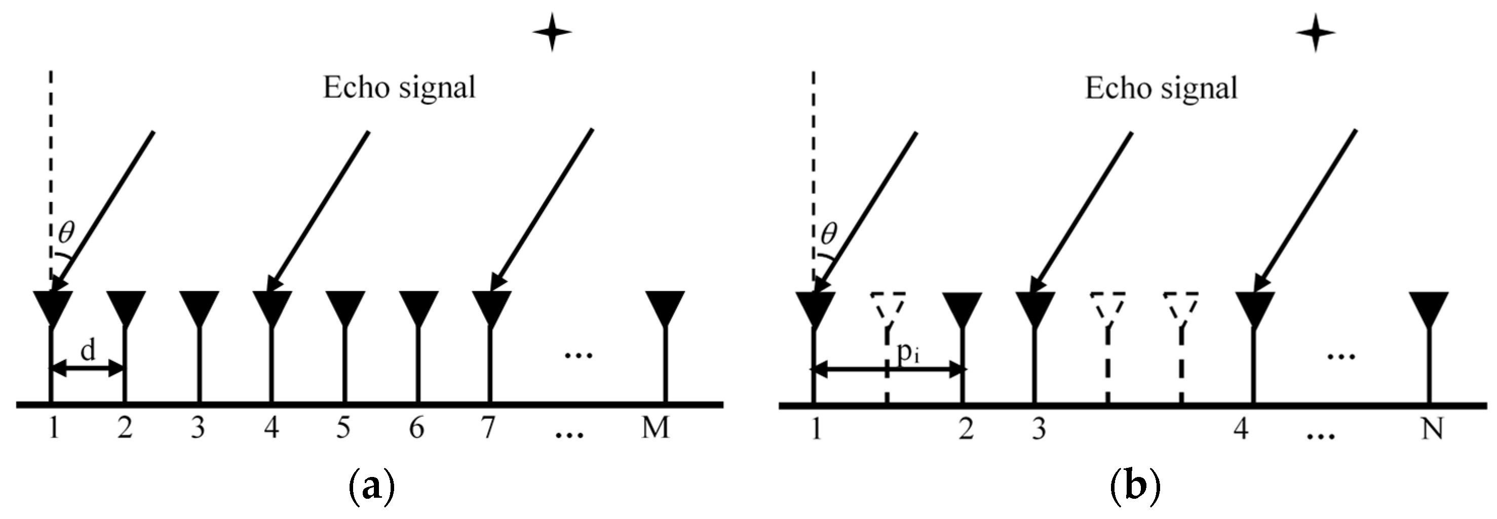
2. Signal Model

Consider a linear array reception system composed of isotropic sensors as shown in Figure 1, which examines both ULA with $M$ elements and SLA with $N$ elements (assuming $N<M$). For the SLA depicted in Figure 1b, sensors outlined with dashed lines indicate positions where no sensor is placed, also referred to as “holes”. The normalized unit element spacing is denoted by $d=\lambda /2$, where $\lambda$ is the carrier wavelength. The set of sensor positions is uniformly denoted as $p_i\in \mathbb{P}=\left\{nd|n\in \mathbb{Z}\right\}$ (in the case of ULA, $n=0,1,2,\dots ,M$, $M$ is the total number of elements), where $\mathbb{Z}$ denotes the set of integers and $p_i$ represents the distance between the $i\mathrm{th}$ element and the reference element. Assumed that there are $K$ far-field narrowband signals impinging on the array from different directions ${\theta }_k$ (for the ULA, generally required that $K<M$), then the $i\mathrm{th}$ element of array output at time $t$ can be expressed as [7,9].

$$y_i(t)={\displaystyle \sum _{k=1}^K{s}_k(t)\exp (j\frac{2\pi }{\lambda }}{p}_i\sin {\theta }_k)+n_i(t)$$

(1)

where $s_k(t)$ is the complex envelope of the $k\mathrm{th}$ signal impinging on the $i\mathrm{th}$ element, $n_i(t)$ is the additive white Gaussian noise at the $i\mathrm{th}$ element, and ${\theta }_k$ is the DOA of the $k\mathrm{th}$ signal. The steering vector of ${\theta }_k$ is defined as

$$\mathit{a}({\theta }_k)={\left[1,\exp (j2\pi \frac{p_2}{\lambda }\sin {\theta }_k),\dots ,\exp (j2\pi \frac{p_{M(N)}}{\lambda }\sin {\theta }_k)\right]}^T.$$

(2)

The $M\times K$ (or $N\times K$ for the SLA case) array steering matrix $\mathit{A}$ with $\mathit{a}({\theta }_k)$ as the $k\mathrm{th}$ $M\times 1$ (or $N\times 1$ for the SLA case) steering vector is defined as $\mathit{A}=[\mathit{a}({\theta }_1),\dots ,\mathit{a}({\theta }_K)]$. Then, the output of $M (or N)$ array elements is $\mathit{y}(t)=\mathit{As}(t)={[y_1(t),\dots ,y_{M(N)}(t)]}^T$. When the array receives $L$ sampling snapshots, the array output can be represented as $\mathit{Y}=[\mathit{y}(t_1),\mathit{y}(t_2),\dots ,\mathit{y}(t_L)]$. For the sake of simplicity, let’s convert that to matrix form:

$$\mathit{Y}=\mathit{AS}+\mathit{N}.$$

(3)

In the formula, $\mathit{Y}$ is the $M\times L (\mathrm{or} N\times L)$ output data matrix, $\mathit{S}=[\mathit{s}(t_1),\dots ,\mathit{s}(t_L)]$ is the signals impinging on the array with dimension, where $\mathit{s}(t_l)={[s_1(t),\dots ,s_K(t)]}^T$ is the signal’s vector at $l\mathrm{th}$ snapshot, and we assume that the source signals are uncorrelated spatially and temporarily. $\mathit{N}=[\mathit{n}(t_1),\dots ,\mathit{n}(t_L)]$ is $M\times L (\mathrm{or} N\times L)$ dimensional Gaussian white noise matrix composed of additive Gaussian white noise with a mean of zero and power of ${\sigma }_n^2$. Moreover, the source signals and the noise are assumed to be uncorrelated with each other. It is noteworthy that, in many parameter estimation models based on sparse recovery, if the array receives a single snapshot (i.e., $L=1$), it typically forms an SMV model, whereas, if the array captures multiple snapshots, it constitutes an MMV model [23].

Then, the covariance matrix of the array output can be defined as

$$\begin{array}{ll}\mathit{R}& =E\left[\mathit{y}(t){\mathit{y}}^H(t)\right]={\displaystyle \sum _{k=1}^K{\sigma }_k^2\mathit{a}({\theta }_k){\mathit{a}}^H({\theta }_k)+{\sigma }_n^2{\mathit{I}}_{M(N)}}\\ & =\mathit{A}diag(\mathit{p}){\mathit{A}}^H+{\sigma }_n^2{\mathit{I}}_{M(N)}.\end{array}$$

(4)

When signals are uncorrelated, $diag(\mathit{p})=E[\mathit{s}(t){\mathit{s}}^H(t)]=diag\{{\sigma }_1^2,{\sigma }_2^2,\dots ,{\sigma }_K^2\}$ denotes the covariance matrix of the signals and ${\sigma }_k^2$ is the power of $k\mathrm{th}$ signal. In practice, the covariance $\mathit{R}$ in (4) is typically approximated by the sample covariance matrix derived from sampling data of array outputs over $L$ snapshots, that is

$$\stackrel{⌢}{\mathit{R}}=\frac{1}{L}{\displaystyle \sum _{l=1}^L\mathit{y}(t_l){\mathit{y}}^H(t_l)}=\frac{1}{L}\mathit{Y}{\mathit{Y}}^H.$$

(5)

Specifically, the element in the $i\mathrm{th}$ row and $j\mathrm{th}$ column of the covariance matrix $\mathit{R}$ can be represented as

$$R_{ij}=E\left[{\mathit{y}}_i(t){\mathit{y}}_j^{\ast }(t)\right]=\{\begin{array}{l}{\displaystyle \sum _{k=1}^K{\sigma }_k^2{e}^{j2\pi (p_i-p_j)\sin {\theta }_k/\lambda }}, i\ne j\\ {\displaystyle \sum _{k=1}^K{\sigma }_k^2{e}^{j2\pi (p_i-p_j)\sin {\theta }_k/\lambda }}+{\sigma }_n^2, i\ne j,\end{array}$$

(6)

where $p_i,p_j\in \mathbb{P}$. It can be observed from the above equation that the second-order statistical measure, the covariance matrix $\mathit{R}$, encompasses the signal information formed by the difference set of any two physical array element positions, with the exponent terms’ position set constituted by the difference between the $i\mathrm{th}$ and $j\mathrm{th}$ physical array elements. Leveraging this characteristic, the virtual array can be constructed through the SLAs, namely the difference co-array, which typically achieves a larger array aperture and DOF but may contain holes. The following Figure 2 illustrates a coprime array and its difference co-array schematic, formed by subarray element counts of (4, 5) [50,51].

Thus, the difference set formed by any two elements in the array can be defined as $\mathbb{D}=\{p_i-p_j|p_i,p_j\in \mathbb{P}\}$, where elements in this set are also referred to as “lags” in the constructed difference co-array. Elements not included in this set (up to the maximum element in the set) are termed as “holes”. Generally, by vectorizing the covariance matrix $\mathit{R}$, removing redundancy, and rearranging elements, the virtual received signal $\mathit{r}$ corresponding to the difference co-array can be obtained as [50]

$$\begin{array}{ll}\mathit{r}& =vec(\mathit{R})=({\mathit{A}}^{\ast }\odot \mathit{A})\mathit{p}+{\sigma }_n^{2}vec({\mathit{I}}_{M(N)})\\ & =\mathit{Bp}+{\sigma }_n^2\mathit{i},\end{array}$$

(7)

where $\mathit{B}={\mathit{A}}^{\ast }\odot \mathit{A}=[{\mathit{a}}^{\ast }({\theta }_1)\otimes \mathit{a}({\theta }_1),{\mathit{a}}^{\ast }({\theta }_2)\otimes \mathit{a}({\theta }_2),\dots ,{\mathit{a}}^{\ast }({\theta }_K)\otimes \mathit{a}({\theta }_K)]$ represents the steering matrix of the difference co-array. Then, $\mathit{p}={[{\sigma }_1^2,{\sigma }_2^2,\dots ,{\sigma }_K^2]}^T$ and $\mathit{i}=vec({\mathit{I}}_{M(N)})$. The received signal of the difference co-array can be regarded as an equivalent single-snapshot array received signal. Typically, continuous lags are utilized in conjunction with mature parameter estimation methods based on ULA for DOA estimation.

3. Methodology of Virtual Aperture Expansion

This section elaborates on the proposed method for virtual array aperture extension based on the covariance fitting criterion. The singularity of the array output's covariance is related to the number of snapshots $L$ and the physical array elements $M(\mathrm{or} N)$, leading to distinct covariance fitting criteria [28]. Simultaneously, scenarios involving both ULAs and SLAs are considered. Therefore, aperture extension is discussed for four scenarios: (1) ULA with more snapshots than elements, (2) ULA with more elements than snapshots, (3) SLA with more snapshots than elements, and (4) SLA with fewer snapshots than elements. Additionally, the relationship between the optimization problems formed using the covariance fitting criterion and ANM in various scenarios is also discussed.

3.1. The Case of ULA when $M<L$

From (4) and (6), when the noise is Gaussian white noise, it is evident that the elements parallel to the main diagonal in the covariance matrix $\mathit{R}$ are identical and elements symmetric to the main diagonal are conjugates of each other. It is thus known that this covariance matrix is a Hermitian PSD Toeplitz matrix [23], which can be specifically represented as

$$\begin{array}{ll}\mathit{R}& =E\left[\mathit{y}(t){\mathit{y}}^H(t)\right]=\mathit{A}diag(\mathit{p}){\mathit{A}}^H+{\sigma }_n^2{\mathit{I}}_{M(N)}\\ & =\mathit{A}diag(\mathit{p}){\mathit{A}}^H+diag({\sigma }_n^2)\\ & ={\mathit{R}}_{\mathit{S}}+{\mathit{R}}_{\mathit{N}}\\ & =T(\mathit{u}),\end{array}$$

(8)

where ${\mathit{R}}_{\mathit{S}}=\mathit{A}diag(\mathit{p}){\mathit{A}}^H$ represents the signal covariance matrix, which is a Hermitian Toeplitz matrix. ${\mathit{R}}_{\mathit{N}}=diag({\sigma }_n^2)$ denotes the covariance matrix composed of noise, forming a diagonal matrix. This covariance matrix can be constructed through the Toeplitzization process $T(•)$ of a vector $\mathit{u}$, where the noise term is added to the first element of $\mathit{u}$, and the other elements of the vector are solely related to the signal terms.

The proposed method for virtual aperture extension of arrays can be regarded as extending $M$ elements of a physical ULA, with the inter-element spacing $d=\lambda /2$, to $M^{\prime }(M^{\prime }>M)$ elements, as illustrated in the schematic shown in Figure 3. The covariance matrix of the array output after extension still satisfies the Toeplitz property and can be represented as

$${\overline{\mathit{R}}}_{\mathit{E}}={\overline{\mathit{R}}}_{\mathit{ES}}+{\overline{\mathit{R}}}_{\mathit{EN}}=T(\mathit{r})+diag({\sigma }_n^2),$$

(9)

where ${\overline{\mathit{R}}}_{\mathit{ES}}=T(\mathit{r})$ and ${\overline{\mathit{R}}}_{\mathit{EN}}=diag({\sigma }_n^2)$ represent the signal covariance matrix and noise covariance matrix, respectively, after the virtual array extension, both of which are $M^{\prime }\times M^{\prime }$ dimensional.

In the case of ULA with more snapshots L than actual physical array elements $M$ (i.e., $L>M$), the sample covariance matrix $\stackrel{⌢}{\mathit{R}}$ of actual array output in (5) is nonsingular. By obtaining an ideal covariance matrix, such as $\mathit{R}$ in (4), from the sample covariance matrix derived through likelihood estimation, one can construct a relationship using the covariance fitting criterion and minimize the following expression to obtain the desired result [29]

$$\begin{array}{ll}\min f_1\left(\mathsf{\theta },\mathit{p},{\sigma }_n^2\right)& ={\Vert {\mathit{R}}^{-\frac{1}{2}}\left(\stackrel{⌢}{\mathit{R}}-\mathit{R}\right){\stackrel{⌢}{\mathit{R}}}^{-\frac{1}{2}}\Vert }_F^2\\ & =Tr\left[{\mathit{R}}^{-\frac{1}{2}}\left(\stackrel{⌢}{\mathit{R}}-\mathit{R}\right){\stackrel{⌢}{\mathit{R}}}^{-1}\left(\stackrel{⌢}{\mathit{R}}-\mathit{R}\right){\mathit{R}}^{-\frac{1}{2}}\right]\\ & =Tr\left[\left({\mathit{R}}^{-1}\stackrel{⌢}{\mathit{R}}-\mathit{I}\right)\left(\mathit{I}-{\stackrel{⌢}{\mathit{R}}}^{-1}\mathit{R}\right)\right]\\ & =Tr\left({\mathit{R}}^{-1}\stackrel{⌢}{\mathit{R}}\right)+Tr\left({\stackrel{⌢}{\mathit{R}}}^{-1}\mathit{R}\right)-2M.\end{array}$$

(10)

The derivation of the fitting criterion in (10) is detailed in Appendix A. It is observed that the covariance matrix $\mathit{R}$ is a nonconvex and nonlinear function with respect to the parameters in $(\mathsf{\theta },\mathit{p},{\sigma }_n^2)$ of interest, making it challenging to solve directly. In the SPICE method, this problem is discretized and can be linearly represented based on zero-order approximation, related to an optimization problem based on the $l1$ norm, though grid-based methods may encounter mismatch issues [28]. Fortunately, since the covariance matrix $\mathit{R}$ in (8) satisfies the Toeplitz property, leveraging the Vandermonde decomposition lemma [22] and the associated compressive sensing framework [29] allows for the construction of a gridless sparse recovery problem for solving the parameters $\mathsf{\theta }$ in the continuous domain. To be specific, the Vandermonde decomposition lemma states that an $M\times M$, rank—$K<M$, positive semidefinite, Toeplitz matrix $T({\mathit{r}}_s)$, which is defined by ${[T({\mathit{r}}_s)]}_{mn}={({\mathit{r}}_s)}_{n-m+1}$, $1\le m\le n\le M$ with ${\mathit{r}}_s\in {ℂ}^M$, combined with (8) can be uniquely decomposed as

$$\begin{array}{l}{\mathit{R}}_{\mathit{S}}=T({\mathit{r}}_s)=\mathit{A}(\mathsf{\theta })diag(\mathit{p}){\mathit{A}}^H(\mathsf{\theta }),\\ \mathit{R}=T({\mathit{r}}_s)+diag({\sigma }_n^2),\end{array}$$

(11)

where certain $\mathit{p}\in {\mathbb{R}}_{+}^K$ and $\theta \in {[-\frac{\pi }{2},\frac{\pi }{2}]}^K$. It can be seen that the covariance matrix $\mathit{R}$ can be reparametrized through using PSD Toeplitz matrix $T({\mathit{r}}_s)$, which is linear with respect to the parameters $({\mathit{r}}_s,{\sigma }_n^2)$. Inserting (11) into (10), we have the following equivalences

$$\begin{array}{l}\underset{{\mathit{r}}_s,\left\{{\sigma }_n^2\ge 0\right\}}{\min } Tr\left({\mathit{R}}^{-1}\stackrel{⌢}{\mathit{R}}\right)+Tr\left({\stackrel{⌢}{\mathit{R}}}^{-1}\mathit{R}\right)-2M, \mathrm{s}.\mathrm{t}. T({\mathit{r}}_s)\ge 0\\ \iff \underset{{\mathit{r}}_s,\left\{{\sigma }_n^2\ge 0\right\}}{\min } Tr\left({\stackrel{⌢}{\mathit{R}}}^{\frac{1}{2}}{\mathit{R}}^{-1}{\stackrel{⌢}{\mathit{R}}}^{\frac{1}{2}}\right)+Tr\left({\stackrel{⌢}{\mathit{R}}}^{-1}\mathit{R}\right), \mathrm{s}.\mathrm{t}. T({\mathit{r}}_s)\ge 0\\ \iff \underset{\mathit{X},{\mathit{r}}_s,\left\{{\sigma }_n^2\ge 0\right\}}{\min } Tr\left(\mathit{X}\right)+Tr\left({\stackrel{⌢}{\mathit{R}}}^{-1}\mathit{R}\right), \mathrm{s}.\mathrm{t}. T({\mathit{r}}_s)\ge 0 \mathrm{and} \mathit{X}\ge {\stackrel{⌢}{\mathit{R}}}^{\frac{1}{2}}{\mathit{R}}^{-1}{\stackrel{⌢}{\mathit{R}}}^{\frac{1}{2}}\\ \iff \underset{\mathit{X},{\mathit{r}}_s,\left\{{\sigma }_n^2\ge 0\right\}}{\min } Tr\left(\mathit{X}\right)+Tr\left({\stackrel{⌢}{\mathit{R}}}^{-1}\mathit{R}\right)\\ \hspace{1em}\mathrm{s}.\mathrm{t}. \left[\begin{array}{ccc}\mathit{X}& {\stackrel{⌢}{\mathit{R}}}^{\frac{1}{2}}& \\ {\stackrel{⌢}{\mathit{R}}}^{\frac{1}{2}}& \mathit{R}& \\ & & T({\mathit{r}}_s)\end{array}\right]\ge 0.\end{array}$$

(12)

In the derivation of the aforementioned formula, the Schur complement theorem is utilized [31], with $\mathit{X}$ as auxiliary variables that satisfies $\mathit{X}\ge {\stackrel{⌢}{\mathit{R}}}^{\frac{1}{2}}{\mathit{R}}^{-1}{\stackrel{⌢}{\mathit{R}}}^{\frac{1}{2}}$. Therefore, the covariance fitting problem is cast as semi-definite programming (SDP) and that is convex. The equivalence between this optimization problem and the one formulated through ANM is elaborated in the derivations found in Appendix B, which demonstrate that the covariance $\mathit{R}$ can be represented using the smallest set of atoms. It is apparent that this optimization problem is solved in the continuous domain rather than being discretized, thereby aiding the accuracy of parameter estimation. As a result, $\mathit{R}$ can be estimated by solving the SDP with its estimate given by $\widehat{\mathit{R}}=T({\hat{\mathit{r}}}_s)+diag({\widehat{\sigma }}_n^2)$, where $({\hat{\mathit{r}}}_s,{\widehat{\sigma }}_n^2)$ is the solution of SDP. Whereas the array extension method proposed still expands virtual elements at equal intervals and the covariance ${\overline{\mathit{R}}}_{\mathit{E}}$ of the virtually extended array in (9) continues to satisfy the PSD Toeplitz property. Drawing from theoretical considerations, the covariance $\mathit{R}$ constituted by the actual physical array should match the corresponding elements in the covariance ${\overline{\mathit{R}}}_{\mathit{E}}$ of the virtually extended array [54]. Specifically, the submatrix formed by the first $M$ rows and the first $M$ columns of ${\overline{\mathit{R}}}_{\mathit{E}}$ should be identical to $\mathit{R}$, with the detailed relationship shown in the following formula

$$\begin{array}{c}\left[{{\overline{\mathit{R}}}_{\mathit{E}}|}_{1:M}^{1:M}\right]=\mathit{R}\\ \nearrow \\ {\overline{\mathit{R}}}_{\mathit{E}}=\left[\begin{array}{l}\boxed{\begin{array}{ccc}\begin{array}{c}{\left({\overline{\mathit{R}}}_{\mathit{E}}\right)}_{1,1}\\ ⋮\\ {\left({\overline{\mathit{R}}}_{\mathit{E}}\right)}_{M,1}\end{array}& \begin{array}{c}\cdots \\ \ddots \\ \cdots \end{array}& \begin{array}{c}{\left({\overline{\mathit{R}}}_{\mathit{E}}\right)}_{1,M}\\ ⋮\\ {\left({\overline{\mathit{R}}}_{\mathit{E}}\right)}_{M,M}\end{array}\end{array}}\begin{array}{c}\cdots \\ \cdots \\ \cdots \end{array}\begin{array}{c}{\left({\overline{\mathit{R}}}_{\mathit{E}}\right)}_{1,M^{\prime }}\\ ⋮\\ {\left({\overline{\mathit{R}}}_{\mathit{E}}\right)}_{M,M^{\prime }}\end{array}\\ \begin{array}{ccccc}\hspace{1em}\hspace{1em}⋮\hspace{1em}\hspace{1em}& \ddots \hspace{1em}\hspace{1em}& ⋮\hspace{1em}\hspace{1em}& \ddots \hspace{1em}& ⋮\hspace{1em}\end{array}\\ \begin{array}{cccc}\begin{array}{cc}{\left({\overline{\mathit{R}}}_{\mathit{E}}\right)}_{M^{\prime },1}& \cdots \end{array}& {\left({\overline{\mathit{R}}}_{\mathit{E}}\right)}_{M^{\prime },M}& \cdots & {\left({\overline{\mathit{R}}}_{\mathit{E}}\right)}_{M^{\prime },M^{\prime }}\end{array}\end{array}\right].\end{array}$$

(13)

Wherein ${{\overline{\mathit{R}}}_{\mathit{E}}|}_{1:M}^{1:M}$ represents the submatrix constituted by the first $M$ rows and the first $M$ columns of the covariance matrix ${\overline{\mathit{R}}}_{\mathit{E}}$. Meanwhile, the noise power of the extended array remains greater than zero. Thus, utilizing (12) allows for the fitting of the covariance $\stackrel{⌢}{\mathit{R}}$ to ${{\overline{\mathit{R}}}_{\mathit{E}}|}_{1:M}^{1:M}$ and simultaneously obtaining the complete covariance matrix ${\overline{\mathit{R}}}_{\mathit{E}}$. This achieves the covariance of a larger aperture ULA from the covariance of the original array output through virtual extension through covariance fitting. Combined with (9), (12) and (13), substituting the submatrix yields the following

$$\begin{array}{ll}\underset{\mathit{r}}{\min } Tr\left({\left[{{\overline{\mathit{R}}}_{\mathit{E}}|}_{1:M}^{1:M}\right]}^{-1}\stackrel{⌢}{\mathit{R}}\right)+Tr\left({\stackrel{⌢}{\mathit{R}}}^{-1}\left[{{\overline{\mathit{R}}}_{\mathit{E}}|}_{1:M}^{1:M}\right]\right)& \iff \underset{\mathit{W},\mathit{r}}{\min } Tr\left(\mathit{W}\right)+Tr\left({\stackrel{⌢}{\mathit{R}}}^{-1}\left[{{\overline{\mathit{R}}}_{\mathit{E}}|}_{1:M}^{1:M}\right]\right)\\ \mathrm{s}.\mathrm{t}. {\overline{\mathit{R}}}_{\mathit{E}}=T(\mathit{r})+diag({\sigma }_n^2)& \mathrm{s}.\mathrm{t}. {\overline{\mathit{R}}}_{\mathit{E}}=T(\mathit{r})+diag({\sigma }_n^2)\\ \hspace{1em}T(\mathit{r})\ge 0& \hspace{1em}T(\mathit{r})\ge 0\\ \hspace{1em}{\sigma }_n^2>0& \hspace{1em}{\sigma }_n^2>0\\ & \hspace{1em}\left[\begin{array}{cc}\mathit{W}& {\stackrel{⌢}{\mathit{R}}}^{\frac{1}{2}}\\ {\stackrel{⌢}{\mathit{R}}}^{\frac{1}{2}}& {{\overline{\mathit{R}}}_{\mathit{E}}|}_{1:M}^{1:M}\end{array}\right]\ge 0.\end{array}$$

(14)

It is clear that the aforementioned equation remains a semi-definite convex optimization problem, which can be solved using various solvers designed for SDP available in CVX, such as sdpt3, SeDuMi, and MOSEK [55]. Utilizing the solution obtained for $\mathit{r}$, the covariance matrix ${\tilde{\mathit{R}}}_E=T(\mathit{r})$ of the extended array can be reconstructed. Applying this covariance matrix for DOA estimation can mitigate the impact of certain noise components, thereby enhancing estimation performance. This covariance matrix can be considered as a low-rank, semi-definite covariance matrix reconstructed in an optimized manner, still adhering to the Vandermonde decomposition. Since the estimated parameters $\mathsf{\theta }$ and the covariance matrix ${\tilde{\mathit{R}}}_E$ have a one-to-one correspondence, DOA estimation can be achieved through frequency retrieval methods (such as MUSIC [4], root-MUSIC [5], Prony's Method [56], Vandermonde decomposition [22], etc.), or directly through covariance-based direction finding techniques like Capon, DBF, etc. [8,9], which are not further elaborated on here.

3.2. The Case of ULA when $M>L$

When the number of array elements $M$ exceeds the number of received snapshots $L$, the sample covariance matrix $\stackrel{⌢}{\mathit{R}}$ becomes singular. To obtain a more ideal covariance $\mathit{R}$, it is known from [28] and [29] that there exists a different covariance fitting criterion compared to the one in the previous section. It can be expressed as

$$\begin{array}{ll}\min f_2\left(\mathsf{\theta },\mathit{p},{\sigma }_n^2\right)& ={\Vert {\mathit{R}}^{-\frac{1}{2}}\left(\stackrel{⌢}{\mathit{R}}-\mathit{R}\right)\Vert }_F^2\\ & =Tr\left[\left(\stackrel{⌢}{\mathit{R}}-\mathit{R}\right){\mathit{R}}^{-1}\left(\stackrel{⌢}{\mathit{R}}-\mathit{R}\right)\right]\\ & =Tr\left(\stackrel{⌢}{\mathit{R}}{\mathit{R}}^{-1}\stackrel{⌢}{\mathit{R}}\right)+Tr\left(\mathit{R}\right)-2Tr\left(\stackrel{⌢}{\mathit{R}}\right).\end{array}$$

(15)

Similarly, it is still challenge to minimize $f_2$ with respect to the unknow interested parameters $\mathsf{\theta },\mathit{p}, \mathrm{and} {\sigma }_n^2$ due to their nonlinear and nonconvex relationship to $\mathit{R}$ according to (4). Similarly, the covariance matrix $\mathit{R}$ still satisfies the Toeplitz property. Based on the Vandermonde lemma [22] and related sparse recovery frameworks [29], and in conjunction with (11), it can be reparametrized and linearly represented using a PSD Toeplitz matrix $T({\mathit{r}}_s)$, resulting in the following

$$\begin{array}{l}\underset{{\mathit{r}}_s,\left\{{\sigma }_n^2\ge 0\right\}}{\min } Tr\left(\stackrel{⌢}{\mathit{R}}{\mathit{R}}^{-1}\stackrel{⌢}{\mathit{R}}\right)+Tr\left(\mathit{R}\right)-2Tr\left(\stackrel{⌢}{\mathit{R}}\right), \mathrm{s}.\mathrm{t}. T({\mathit{r}}_s)\ge 0\\ \iff \underset{\mathit{X},{\mathit{r}}_s,\left\{{\sigma }_n^2\ge 0\right\}}{\min } Tr\left(\mathit{X}\right)+Tr\left(\mathit{R}\right)\\ \hspace{1em}\mathrm{s}.\mathrm{t}. \left[\begin{array}{ccc}\mathit{X}& \stackrel{⌢}{\mathit{R}}& \\ \stackrel{⌢}{\mathit{R}}& \mathit{R}& \\ & & T({\mathit{r}}_s)\end{array}\right]\ge 0.\end{array}$$

(16)

The derivation of the above formula also utilizes the Schur complement theorem [31]. It forms a convex SDP problem that can be solved in the continuous domain. The connection between this and optimization problems constructed based on ANM is briefly explained in Appendix C. Similarly, to obtain the covariance ${\tilde{\mathit{R}}}_E$ of the extended array, based on explanations from the previous section and in conjunction with (9) and (13), the following semi-definite convex optimization problem can be formulated for solution

$$\begin{array}{ll}\underset{\mathit{r}}{\min } Tr\left(\stackrel{⌢}{\mathit{R}}{\left[{{\overline{\mathit{R}}}_{\mathit{E}}|}_{1:M}^{1:M}\right]}^{-1}\stackrel{⌢}{\mathit{R}}\right)+Tr\left({{\overline{\mathit{R}}}_{\mathit{E}}|}_{1:M}^{1:M}\right)& \iff \underset{\mathit{W},\mathit{r}}{\min } Tr\left(\mathit{W}\right)+Tr\left({{\overline{\mathit{R}}}_{\mathit{E}}|}_{1:M}^{1:M}\right)\\ \mathrm{s}.\mathrm{t}. {\overline{\mathit{R}}}_{\mathit{E}}=T(\mathit{r})+diag({\sigma }_n^2)& \mathrm{s}.\mathrm{t}. {\overline{\mathit{R}}}_{\mathit{E}}=T(\mathit{r})+diag({\sigma }_n^2)\\ \hspace{1em}T(\mathit{r})\ge 0& \hspace{1em}T(\mathit{r})\ge 0\\ \hspace{1em}{\sigma }_n^2>0& \hspace{1em}{\sigma }_n^2>0\\ & \hspace{1em}\left[\begin{array}{cc}\mathit{W}& \stackrel{⌢}{\mathit{R}}\\ \stackrel{⌢}{\mathit{R}}& {{\overline{\mathit{R}}}_{\mathit{E}}|}_{1:M}^{1:M}\end{array}\right]\ge 0.\end{array}$$

(17)

The above equation can also be solved using CVX solvers [55] designed for SDP problems. Once $\mathit{r}$ for the extended array is obtained, the covariance matrix ${\tilde{\mathit{R}}}_E=T(\mathit{r})$ can be constructed for DOA estimation, utilizing frequency retrieval or covariance matrix-based direction-finding methods.

3.3. The Case of SLA when $N<L$

Typically, the SLA can be considered as derived by selecting a subset of elements from the ULA [23]. We can denote that the set of the indices of the sensors is $\mathsf{\Omega }\subset \left\{1,2,\dots ,M\right\}$ and let $N$ be the cardinality of $\mathsf{\Omega }$ (i.e., the elements number of the SLA). Correspondingly, only the rows of $\mathit{Y}$ indexed by $\mathsf{\Omega }$ are observed from the array output of the full ULA and form an $N\times L$ data matrix ${\mathit{Y}}_{\mathsf{\Omega }}={\mathsf{\Gamma }}_{\mathsf{\Omega }}\mathit{Y}$, where $\mathsf{\Gamma }\in {\left\{0,1\right\}}^{N\times M}$ is the row-selection matrix that has ones at the $(j,{\mathsf{\Omega }}_j)\mathrm{th}$ entries, $j=1,\dots ,N$ and zeros elsewhere. At this point, the steering matrix of the SLA, denoted as ${\mathit{A}}_{\mathsf{\Omega }}={\mathsf{\Gamma }}_{\mathsf{\Omega }}\mathit{A}=[{\mathit{a}}_{\mathsf{\Omega }}({\theta }_1),\dots ,{\mathit{a}}_{\mathsf{\Omega }}({\theta }_K)]\in {ℂ}^{N\times K}$, can be obtained by indexing the steering matrix of the full ULA using the index set $\mathsf{\Omega }$ [30]. Specifically, the covariance matrix of the SLA can be represented as

$$\begin{array}{ll}{\mathit{R}}_{\mathsf{\Omega }}& =E\left[{\mathit{y}}_{\mathsf{\Omega }}(t){\mathit{y}}_{\mathsf{\Omega }}{(t)}^H\right]={\mathsf{\Gamma }}_{\mathsf{\Omega }}E\left[\mathit{y}(t)\mathit{y}{(t)}^H\right]{\mathsf{\Gamma }}_{\mathsf{\Omega }}^T={\mathsf{\Gamma }}_{\mathsf{\Omega }}\mathit{R}{\mathsf{\Gamma }}_{\mathsf{\Omega }}^T\\ & ={\mathit{A}}_{\mathsf{\Omega }}diag(\mathit{p}){\mathit{A}}_{\mathsf{\Omega }}+diag\left({\left[{\sigma }_n^2\right]}_{\mathsf{\Omega }}\right).\end{array}$$

(18)

Herein, ${\mathit{y}}_{\mathsf{\Omega }}(t)$ represents the echo signal received by the SLA at time $t$, which can also be obtained by indexing the received signals of the full ULA using the index set $\mathsf{\Omega }$. $\mathit{p}={[{\sigma }_1^2,{\sigma }_2^2,\dots ,{\sigma }_K^2]}^T$ denotes the power of signals. Typically in practice, the covariance in (18) is approximated using maximum likelihood estimation based on multiple snapshots collected by the array, expressed as

$${\stackrel{⌢}{\mathit{R}}}_{\mathsf{\Omega }}=\frac{1}{L}{\displaystyle \sum _{l=1}^L{\mathit{y}}_{\mathsf{\Omega }}(t_l){\mathit{y}}_{\mathsf{\Omega }}^H(t_l)}=\frac{1}{L}{\mathit{Y}}_{\mathsf{\Omega }}{\mathit{Y}}_{\mathsf{\Omega }}^H.$$

(19)

Analogously, given ${\stackrel{⌢}{\mathit{R}}}_{\mathsf{\Omega }}$, to estimate ${\mathit{R}}_{\mathsf{\Omega }}$, we can also consider using covariance fitting criteria to fit it as follows [30]

$$\min f_3\left(\mathsf{\theta },\mathit{p},{\sigma }_n^2\right)={\Vert {\mathit{R}}_{\mathsf{\Omega }}^{-\frac{1}{2}}\left({\stackrel{⌢}{\mathit{R}}}_{\mathsf{\Omega }}-{\mathit{R}}_{\mathsf{\Omega }}\right){\stackrel{⌢}{\mathit{R}}}_{\mathsf{\Omega }}^{-\frac{1}{2}}\Vert }_F^2=Tr\left({\mathit{R}}_{\mathsf{\Omega }}^{-1}{\stackrel{⌢}{\mathit{R}}}_{\mathsf{\Omega }}\right)+Tr\left({\stackrel{⌢}{\mathit{R}}}_{\mathsf{\Omega }}^{-1}{\mathit{R}}_{\mathsf{\Omega }}\right)-c_1,$$

(20)

where $c_1$ denotes the constant. Then, from (18), it can be inferred that the covariance matrix ${\mathit{R}}_{\mathsf{\Omega }}$ for the SLA is a submatrix of the covariance $\mathit{R}$ for the ULA. Therefore, using the parameterization of $\mathit{R}$ as in (11), ${\mathit{R}}_{\mathsf{\Omega }}$ can be linearly parameterized as

$$\begin{array}{ll}{\mathit{R}}_{\mathsf{\Omega }}& \triangleq {\mathit{A}}_{\mathsf{\Omega }}(\mathsf{\theta })diag(\mathit{p}){\mathit{A}}_{\mathsf{\Omega }}^H(\mathsf{\theta })+diag\left({\left[{\sigma }_n^2\right]}_{\mathsf{\Omega }}\right)\\ & ={\mathsf{\Gamma }}_{\mathsf{\Omega }}T({\mathit{r}}_s){\mathsf{\Gamma }}_{\mathsf{\Omega }}^T+diag\left({\left[{\sigma }_n^2\right]}_{\mathsf{\Omega }}\right)\\ & ={\left[{\mathit{R}}_{\mathit{S}}\right]}_{\mathsf{\Omega }}+{\left[{\mathit{R}}_{\mathit{N}}\right]}_{\mathsf{\Omega }}.\end{array}$$

(21)

From the above, it is known that the signal covariance matrix ${\left[{\mathit{R}}_{\mathit{S}}\right]}_{\mathsf{\Omega }}$ constructed through the selection matrix ${\mathsf{\Gamma }}_{\mathsf{\Omega }}$ is in a one-to-one mapping relationship with the signal covariance matrix ${\mathit{R}}_{\mathit{S}}$ formed from the full ULA. And in the case of $L>M$, ${\stackrel{⌢}{\mathit{R}}}_{\mathsf{\Omega }}$ is still nonsingular. Additionally, $T({\mathit{r}}_s)$ satisfies the Hermitian PSD Toeplitz property, and ${\left[{\sigma }_n^2\right]}_{\mathsf{\Omega }}\ge 0$. Therefore, from Section 3.1 and combined with (20), we can construct the following SDP problem for solving in the continuous domain in the case of SLA

$$\begin{array}{l}\underset{{\mathit{r}}_s,\left\{{\left[{\sigma }_n^2\right]}_{\mathsf{\Omega }}\ge 0\right\}}{\min } Tr\left({\mathit{R}}_{\mathsf{\Omega }}^{-1}{\stackrel{⌢}{\mathit{R}}}_{\mathsf{\Omega }}\right)+Tr\left({\stackrel{⌢}{\mathit{R}}}_{\mathsf{\Omega }}^{-1}{\mathit{R}}_{\mathsf{\Omega }}\right)-c_1, \mathrm{s}.\mathrm{t}. T({\mathit{r}}_s)\ge 0\\ \iff \underset{\mathit{X},{\mathit{r}}_s,\left\{{\left[{\sigma }_n^2\right]}_{\mathsf{\Omega }}\ge 0\right\}}{\min } Tr\left(\mathit{X}\right)+Tr\left({\stackrel{⌢}{\mathit{R}}}_{\mathsf{\Omega }}^{-1}{\mathit{R}}_{\mathsf{\Omega }}\right)\\ \hspace{1em}\mathrm{s}.\mathrm{t}. \left[\begin{array}{ccc}\mathit{X}& {\stackrel{⌢}{\mathit{R}}}_{\mathsf{\Omega }}^{\frac{1}{2}}& \\ {\stackrel{⌢}{\mathit{R}}}_{\mathsf{\Omega }}^{\frac{1}{2}}& {\mathit{R}}_{\mathsf{\Omega }}& \\ & & T({\mathit{r}}_s)\end{array}\right]\ge 0.\end{array}$$

(22)

Once the above SDP is solved, $\mathit{R}$ can be estimated by $\widehat{\mathit{R}}=T({\hat{\mathit{r}}}_s)+diag({\widehat{\sigma }}_n^2)$, where $({\hat{\mathit{r}}}_s,{\widehat{\sigma }}_n^2)$ is the solution of SDP. The connection between the optimization problem constructed in this scenario and ANM is briefly explained in Appendix D. It is notable that, under certain conditions, the sample covariance matrix ${\stackrel{⌢}{\mathit{R}}}_{\mathsf{\Omega }}$ obtained from the sparse array output can be fitted to derive the covariance $\widehat{\mathit{R}}$ of the full ULA, meaning that the full matrix $T({\mathit{r}}_s)$ can be obtained through the submatrix ${\mathsf{\Gamma }}_{\mathsf{\Omega }}T({\mathit{r}}_s){\mathsf{\Gamma }}_{\mathsf{\Omega }}^T$. This implies that the final parameter estimation is akin to an estimation under the scenario of a full ULA, with all the DOA information contained within the Toeplitz matrix $T({\hat{\mathit{r}}}_s)$ recovered through sparse reconstruction, which contributes to enhance estimation performance. In detail, it is recognized that ULAs and many SLAs exhibit redundancy. The estimator based on such SDP is statistically consistent in the snapshot number $L$ when source number $K\le M-1$. To see this, let us consider the ULA case first. As $L$ increases indefinitely, the sample covariance matrix $\stackrel{⌢}{\mathit{R}}$ tends towards the true data covariance matrix that is denoted by ${\mathit{R}}^O$, which retains the same Toeplitz structure as $\mathit{R}$. Consequently, it follows from (10) that $\widehat{\mathit{R}}={\mathit{R}}^O$ and the true parameters are retrievable from $\widehat{\mathit{R}}$. For the SLA, similarly, the covariance matrix estimate ${\widehat{\mathit{R}}}_{\mathsf{\Omega }}$ likewise converges to the true covariance as $L\to \infty$. Under the redundancy assumption, all the information necessary for frequency retrieval contained in the Toeplitz matrix $T({\mathit{r}}_s)$ can be deduced from ${\widehat{\mathit{R}}}_{\mathsf{\Omega }}$ and hence that the true parameters can be obtained [23].

Remark: When the SLA $\mathsf{\Omega }$ is not a redundancy array, i.e., the co-array $\mathbb{D}$ is not formed as the ULA. The above estimator can be applied straightforwardly. In such a case, it is natural to require that $K\le \overline{M}-1\le M-1$, where $\overline{M}-1$ denotes the maximum detectable number of sources using the non-redundancy SLA [29].

The case of SLA under virtual array expansion is shown in Figure 4, where $N_U$ denotes the number of elements in the ULA with the same aperture as the SLA, while $N^{\prime }$ represents the total number of elements after expanding the array elements at unit intervals. Unlike the situation with ULA, there are intervals where no array elements exist. Thus, it becomes necessary to first virtually fill the positions of these holes. However, as previously indicated, the covariance matrix ${\stackrel{⌢}{\mathit{R}}}_{\mathsf{\Omega }}$ outputted by the SLA can be approximated to obtain a covariance matrix $\widehat{\mathit{R}}$ similar to that of ULA, essentially “interpolating” within unit intervals to fill the holes and achieve the covariance of virtual ULA. When considering the expansion of the array, the virtual array elements are still expanded at unit intervals. If the covariance matrix after expansion is denoted as ${\overline{\mathit{R}}}_E\in {\mathbb{C}}^{N^{\prime }\times N^{\prime }}$, it still satisfies (9). Theoretically, for the cross-correlation obtained from the physical array output of known position elements and the covariance of the expanded array at corresponding positions (i.e., the elements at corresponding positions in the submatrix ${\mathit{R}}_{\mathsf{\Omega }}$ are the coincident as those in the expanded array covariance), we can re-parameterize and linearly characterize ${\overline{\mathit{R}}}_E$ through ${\mathit{r}}_{\mathsf{\Omega }}$ ($\mathit{r}$ is indexed with $\mathsf{\Omega }$), similar to the description in Section 3.1 and combined with (22), leading to the SDP problem expressed in (23). The relationship between the submatrix ${\mathit{R}}_{\mathsf{\Omega }}$ and the expanded matrix ${\overline{\mathit{R}}}_E$ is shown in (24).

$$\begin{array}{l}\underset{r}{\min }Tr\left({\left[{\left.{\mathsf{\Gamma }}_{\mathsf{\Omega }}{\overline{\mathit{R}}}_{\mathit{E}}\right|}_{1:N_U}^{1:N_U}{\mathsf{\Gamma }}_{\mathsf{\Omega }}^{\tau }\right]}^{-1}{\widehat{\mathit{R}}}_{\mathsf{\Omega }}\right)+Tr\left({\mathsf{\Gamma }}_{\mathsf{\Omega }}^{\tau }{\widehat{\mathit{R}}}_{\mathsf{\Omega }}^{-1}{\mathsf{\Gamma }}_{\mathsf{\Omega }}\left[{\left.{\overline{\mathit{R}}}_{\mathit{E}}\right|}_{1:N_U}^{1:N_U}\right]\right)\\ \mathrm{s}.\mathrm{t}.{\overline{\mathit{R}}}_{\mathit{E}}=T\left(\mathit{r}\right)+diag\left({\sigma }_n^2\right)\\ \hspace{1em}T\left(\mathit{r}\right)\ge 0\\ \hspace{1em}{\sigma }_n^2>0\\ \iff \underset{\mathit{W},r}{\min }Tr\left(\mathit{W}\right)+Tr\left({\mathsf{\Gamma }}_{\mathsf{\Omega }}^T{\widehat{\mathit{R}}}_{\mathsf{\Omega }}^{-1}{\mathsf{\Gamma }}_{\mathsf{\Omega }}\left[{\overline{\mathit{R}}}_{\mathit{E}}^{1{\mathbb{I}}_{1:N_U}}\right]\right)\\ \mathrm{s}.\mathrm{t}.{\overline{\mathit{R}}}_{\mathit{E}}=T\left(\mathit{r}\right)+diag\left({\sigma }_n^2\right)\\ \hspace{1em}T\left(\mathit{r}\right)\ge 0\\ \hspace{1em}{\sigma }_n^2>0\\ \hspace{1em}\left[\begin{array}{cc}\mathit{W}& {\widehat{\mathit{R}}}_{\mathsf{\Omega }}^{\frac{1}{2}}\\ {\widehat{\mathit{R}}}_{\mathsf{\Omega }}^{\frac{1}{2}}& {\mathsf{\Gamma }}_{\mathsf{\Omega }}{\overline{\mathit{R}}}_{\mathit{E}}{|}_{1:N{N}_U}^{1N_U}{\mathsf{\Gamma }}_{\mathsf{\Omega }}^T\end{array}\right]\ge 0\end{array}$$

(23)

$$\begin{array}{l}\left[{{\overline{\mathit{R}}}_{\mathit{E}}|}_{1:N_U}^{1:N_U}=\mathit{R}\right]=\left[\begin{array}{ccccc}{\left(\mathit{R}\right)}_{1,1}& \cdots & 0& \cdots & {\left(\mathit{R}\right)}_{1,N}\\ {\left(\mathit{R}\right)}_{2,1}& \cdots & \cdots & \cdots & {\left(\mathit{R}\right)}_{2,N}\\ ⋮& \cdots & 0& \cdots & ⋮\\ 0& \cdots & \cdots & \cdots & 0\\ {\left(\mathit{R}\right)}_{N,1}& \cdots & 0& \cdots & {\left(\mathit{R}\right)}_{N,N}\end{array}\right]\to {\mathit{R}}_{\mathsf{\Omega }}={\mathsf{\Gamma }}_{\mathsf{\Omega }}\mathit{R}{\mathsf{\Gamma }}_{\mathsf{\Omega }}=\left[\begin{array}{cccc}{\left(\mathit{R}\right)}_{1,1}& \cdots & \cdots & {\left(\mathit{R}\right)}_{1,N}\\ {\left(\mathit{R}\right)}_{2,1}& \ddots & \cdots & {\left(\mathit{R}\right)}_{2,N}\\ ⋮& \cdots & \ddots & ⋮\\ {\left(\mathit{R}\right)}_{N,1}& \cdots & \cdots & {\left(\mathit{R}\right)}_{N,N}\end{array}\right]\\ \nearrow {{\overline{\mathit{R}}}_{\mathit{E}}|}_{1:N_U}^{1:N_U}\\ {\overline{\mathit{R}}}_{\mathit{E}}=\left[\begin{array}{l}\boxed{\begin{array}{ccc}\begin{array}{c}{\left({\overline{\mathit{R}}}_{\mathit{E}}\right)}_{1,1}\\ ⋮\\ {\left({\overline{\mathit{R}}}_{\mathit{E}}\right)}_{N_U,1}\end{array}& \begin{array}{c}\cdots \\ \ddots \\ \cdots \end{array}& \begin{array}{c}{\left({\overline{\mathit{R}}}_{\mathit{E}}\right)}_{1,N_U}\\ ⋮\\ {\left({\overline{\mathit{R}}}_{\mathit{E}}\right)}_{N_U,N_U}\end{array}\end{array}}\begin{array}{c}\cdots \\ \cdots \\ \cdots \end{array}\begin{array}{c}{\left({\overline{\mathit{R}}}_{\mathit{E}}\right)}_{1,N^{\prime }}\\ ⋮\\ {\left({\overline{\mathit{R}}}_{\mathit{E}}\right)}_{N_U,N^{\prime }}\end{array}\\ \begin{array}{ccccc} \hspace{1em}\hspace{1em}⋮\hspace{1em}\hspace{1em}& \ddots \hspace{1em}\hspace{1em}& ⋮\hspace{1em}\hspace{1em}& \ddots \hspace{1em}& ⋮\hspace{1em}\end{array}\\ \begin{array}{cccc}\begin{array}{cc}{\left({\overline{\mathit{R}}}_{\mathit{E}}\right)}_{N^{\prime },1}& \cdots \end{array}& {\left({\overline{\mathit{R}}}_{\mathit{E}}\right)}_{N^{\prime },N_U}& \cdots & {\left({\overline{\mathit{R}}}_{\mathit{E}}\right)}_{N^{\prime },N^{\prime }}\end{array}\end{array}\right]\end{array}$$

(24)

This can be solved using the CVX solver [55] to obtain the estimate of $\mathit{r}$ as $\hat{\mathit{r}}$, which allows for the reconstruction of a low-rank semi-definite Toeplitz covariance matrix ${\tilde{\mathit{R}}}_E=T(\hat{\mathit{r}})$. This matrix can be regarded as virtually completing the missing position elements of the covariance matrix of the SLA when forming the covariance of the ULA. Furthermore, the array is expanded to achieve the covariance of a virtual ULA with a larger aperture, thereby enhancing the performance of effective DOA estimation. This embodies the concept of both “interpolation” and “extrapolation” of array elements. Finally, this covariance can be used with frequency retrieval or covariance matrix-based direction-finding methods to obtain DOA estimates without ambiguity.

3.4. The Case of SLA when $N>L$

In this case, unlike the previous section, the sample covariance matrix ${\stackrel{⌢}{\mathit{R}}}_{\mathsf{\Omega }}$ is singular. By performing covariance fitting, a more ideal estimation of ${\mathit{R}}_{\mathsf{\Omega }}$ can be achieved, which follows [30]

$$\min f_4\left(\mathsf{\theta },\mathit{p},{\sigma }_n^2\right)={\Vert {\mathit{R}}_{\mathsf{\Omega }}^{-\frac{1}{2}}\left({\stackrel{⌢}{\mathit{R}}}_{\mathsf{\Omega }}-{\mathit{R}}_{\mathsf{\Omega }}\right)\Vert }_F^2=Tr\left({\stackrel{⌢}{\mathit{R}}}_{\mathsf{\Omega }}{\mathit{R}}_{\mathsf{\Omega }}^{-1}{\stackrel{⌢}{\mathit{R}}}_{\mathsf{\Omega }}\right)+Tr\left({\mathit{R}}_{\mathsf{\Omega }}\right)-c_2,$$

(25)

where $c_2$ denotes the constant. Since ${\mathit{R}}_{\mathsf{\Omega }}={\mathsf{\Gamma }}_{\mathsf{\Omega }}\mathit{R}{\mathsf{\Gamma }}_{\mathsf{\Omega }}^T$ is a submatrix of the covariance matrix $\mathit{R}$ for the ULA with the same aperture of the SLA, similarly, in conjunction with (21), we know that this submatrix can be linearly represented by a reparametrized covariance matrix $\mathit{R}$ that satisfies the Hermitian PSD Toeplitz property. Similarly, we can obtain the following semi-definite convex optimization problem that is solved in the continuous domain

$$\begin{array}{l}\underset{{\mathit{r}}_s,\left\{{\left[{\sigma }_n^2\right]}_{\mathsf{\Omega }}\ge 0\right\}}{\min } Tr\left({\stackrel{⌢}{\mathit{R}}}_{\mathsf{\Omega }}{\mathit{R}}_{\mathsf{\Omega }}^{-1}{\stackrel{⌢}{\mathit{R}}}_{\mathsf{\Omega }}\right)+Tr\left({\mathit{R}}_{\mathsf{\Omega }}\right)-c_2, \mathrm{s}.\mathrm{t}. T({\mathit{r}}_s)\ge 0\\ \iff \underset{\mathit{X},{\mathit{r}}_s,\left\{{\left[{\sigma }_n^2\right]}_{\mathsf{\Omega }}\ge 0\right\}}{\min } Tr\left(\mathit{X}\right)+Tr\left({\mathit{R}}_{\mathsf{\Omega }}\right)\\ \hspace{1em}\mathrm{s}.\mathrm{t}. \left[\begin{array}{ccc}\mathit{X}& {\stackrel{⌢}{\mathit{R}}}_{\mathsf{\Omega }}& \\ {\stackrel{⌢}{\mathit{R}}}_{\mathsf{\Omega }}& {\mathit{R}}_{\mathsf{\Omega }}& \\ & & T({\mathit{r}}_s)\end{array}\right]\ge 0.\end{array}$$

(26)

Once the above SDP is solved, an estimate of the Toeplitz covariance matrix $T({\hat{\mathit{r}}}_s)$ akin to that formed by a ULA can be constructed. A brief explanation of the relationship between the estimator based on this SDP and ANM is provided in Appendix E. Similarly, theoretically, due to the consistency of the elements in the extended covariance matrix ${\overline{\mathit{R}}}_E$ with those at corresponding positions in the known physical array, and given that the extended covariance matrix still constitutes a virtual ULA with a larger aperture and satisfies the Hermitian PSD Toeplitz property, it can be reparametrized and linearly represented. Consequently, the following semi-definite convex optimization problem can be formulated to obtain an estimate of the extended covariance matrix.

$$\begin{array}{l}\underset{\mathit{r}}{\min } Tr\left({\stackrel{⌢}{\mathit{R}}}_{\mathsf{\Omega }}{\left[{{\mathsf{\Gamma }}_{\mathsf{\Omega }}{\overline{\mathit{R}}}_{\mathit{E}}|}_{1:N_U}^{1:N_U}{\mathsf{\Gamma }}_{\mathsf{\Omega }}^T\right]}^{-1}{\stackrel{⌢}{\mathit{R}}}_{\mathsf{\Omega }}\right)+Tr\left({{\mathsf{\Gamma }}_{\mathsf{\Omega }}{\overline{\mathit{R}}}_{\mathit{E}}|}_{1:N_U}^{1:N_U}{\mathsf{\Gamma }}_{\mathsf{\Omega }}^T\right)\\ \mathrm{s}.\mathrm{t}. {\overline{\mathit{R}}}_{\mathit{E}}=T(\mathit{r})+diag({\sigma }_n^2)\\ \hspace{1em}T(\mathit{r})\ge 0\\ \hspace{1em}{\sigma }_n^2>0\\ \underset{\mathit{W},\mathit{r}}{\iff \min } Tr\left(\mathit{W}\right)+Tr\left({\mathsf{\Gamma }}_{\mathsf{\Omega }}^T{\mathsf{\Gamma }}_{\mathsf{\Omega }}\left[{{\overline{\mathit{R}}}_{\mathit{E}}|}_{1:N_U}^{1:N_U}\right]\right)\\ \mathrm{s}.\mathrm{t}. {\overline{\mathit{R}}}_{\mathit{E}}=T(\mathit{r})+diag({\sigma }_n^2)\\ \hspace{1em}T(\mathit{r})\ge 0\\ \hspace{1em}{\sigma }_n^2>0\\ \hspace{1em}\left[\begin{array}{cc}\mathit{W}& {\stackrel{⌢}{\mathit{R}}}_{\mathsf{\Omega }}\\ {\stackrel{⌢}{\mathit{R}}}_{\mathsf{\Omega }}& {{\mathsf{\Gamma }}_{\mathsf{\Omega }}{\overline{\mathit{R}}}_{\mathit{E}}|}_{1:N_U}^{1:N_U}{\mathsf{\Gamma }}_{\mathsf{\Omega }}^T\end{array}\right]\ge 0\end{array}$$

(27)

The above SDP can be solved using the CVX solver [55] to obtain the estimate of $\mathit{r}$ as $\hat{\mathit{r}}$, which allows for the reconstruction of a Toeplitz covariance matrix $T(\hat{\mathit{r}})$ that represents a virtual ULA with enlarged aperture. This matrix, composed solely of signal components, can then be used for DOA estimation, either through frequency retrieval or covariance-based direction-finding methods. Although the virtual aperture of the array is effectively extended to enhance estimation capabilities in this scenario, the total amount of information remains limited due to the small number of snapshots collected and the sparse array configuration. Consequently, although the estimation performance is improved through sparse recovery of the virtual array's covariance estimate, it is still not perfect compared to situations with a larger amount of information, as the estimation is a little biased.

Up to now, virtual array aperture extension methods based on the covariance fitting criterion have been proposed for four different scenarios. It is evident that all methods involve constructing a larger aperture virtual ULA’s covariance through fitting optimization problems and integrating relevant DOA estimators to achieve improved estimation resolution and accuracy. It should be noted that these methods extend the array by building fitting optimization problems based on the actual array’s sample covariance matrix. The extended array’s covariance matrix contains the same target information as the actual array; thus, theoretically, the amount of information remains constant. Therefore, these methods do not increase the DOF, meaning the number of detectable targets is still limited by the original actual array’s DOF. However, enhancing estimation performance even slightly for actual arrays with commonly encountered small apertures holds significant value.

4. Experiment Results

In this section, some simulations are given under four different scenarios for both ULA and SLA to demonstrate the effectiveness of the method proposed in this paper and to compare it with similar methods to illustrate the estimation performance of the proposed method.

4.1. Simulations for the ULA Case

Numerical examples are provided for two scenarios under the ULA (i.e., when snapshots $L>\mathrm{array} \mathrm{elements} M$ and $L<M$.) case to evaluate the methods’ performance. The comparison methods include MUSIC based on the original physical array output [5], interpolation techniques combined with MUSIC estimator [42] (named IT-MUSIC), a FOC matrix combined with MUSIC estimator (named FOC-MUSIC, also known as MUSIC-LIKE, mentioned in [45,47]), enhanced array extension technique combined with MUSIC estimator [40] (named EE-MUSIC), and FOC-ANM from [46]. To uniformly measure performance, all methods ultimately employ the MUSIC estimator for estimation. The performance of the method is measured by the Root Mean Square Error (RMSE), for which the definition is provided here

$$RMSE=\sqrt{\frac{1}{KQ}{\displaystyle \sum _{k=1}^K{\displaystyle \sum _{q=1}^Q{\left[{\widehat{\theta }}_k\left(q\right)-{\theta }_k\right]}^2}}}.$$

(28)

In the above formula, $K$ is the total number of signal sources and $Q$ is the Monte Carlo runs. ${\widehat{\theta }}_k(q)$ is the estimated DOA value of ${\theta }_k$ in the $q\mathrm{th}$ Monte Carlo experiment and ${\theta }_k$ is the true DOA value of the $k\mathrm{th}$ signal source.

Assuming scenario (a) occurs when $L>M$, the array reception system consists of a ULA with $M=10$ array elements, receiving $L=128$ sampling snapshots. Scenario (b) occurs when $L<M$, where the array reception system is a ULA with $M=16$ elements, receiving $L=8$ sampling snapshots.

Firstly, a simulation demonstrating the effectiveness of the estimation method is provided. In scenario (a), with incoming wave directions at $\mathsf{\theta }=[1^{\circ },4^{\circ }]$, the proposed method extends virtually to 30 elements, while in scenario (b), with directions at $\mathsf{\theta }=[1^{\circ },6^{\circ }]$, it extends to 40 elements (the directions of arrival are within one beamwidth, with the former being more severe as it falls within half a beamwidth. The latter scenario considers a larger angular separation due to the fewer snapshots received, resulting in less overall information). For the other methods in these two scenarios, both IT-MUSIC and EE-MUSIC methods virtually extend to 40 elements. For FOC-MUSIC, the number of virtual elements after redundancy removal can reach at $2M-1$ (the method used did not remove redundancy; therefore, the overlapping part is also utilized), and in FOC-ANM, the number of virtual elements can reach $4M-3$. SNR = 10 dB for both scenarios. These conditions pose a significant challenge to the estimation methods. The spatial spectrum of each method is shown in Figure 5 reveals that the proposed method produces sharp and clear peaks, closely matching the true directions of arrival. In contrast, some methods exhibit blurred peaks, failing to effectively distinguish between the two sources. Under such simulation conditions, the proposed method has demonstrated its effectiveness in estimation.

To further illustrate the array extension performance of the proposed method, assuming the signal’s arrival directions are $\mathsf{\theta }=[0^{\circ },{15}^{\circ }]$ with SNR = 10 dB. Figure 6 and Figure 7, respectively, display the spectrum of Capon and MUSIC as the number of virtual extension elements increases in both scenarios (the “Original recovery” in the figures refers to the covariance of the original array output reconstructed by the proposed method without array extension, similar to SPA [29]).

From Figure 6, it can be observed that, regardless of the scenario, as the number of virtual elements increases, the main-to-side lobe ratio of the Capon spectrum continuously grows, and the main lobe becomes increasingly narrower. In Figure 7, the MUSIC spectrum, with the increase in virtual elements, shows sharper and narrower spectral peaks and the spectral lines between the peaks become more stable. This corroborates that as the number of virtual elements increases, the aperture is enhanced, aiding in improved resolution and estimation performance. However, overall, the estimation performance does not continually increase with the addition of more virtual elements, showing a certain “saturation” and “tempering” trend. Further simulations were conducted to compare the RMSE versus SNRs with varying numbers of virtual extension elements for the proposed method. The directions of arrival in the simulation experiments remain the same as in the first experiment of this section. The SNR ranges from −10 dB to 20 dB in 5 dB steps, with 300 Monte Carlo simulations performed at each SNR. The resulting RMSE curves for different virtual extensions versus SNR are shown in Figure 8. It can be observed that with the continuous increase in the number of virtual elements, the effective SNR threshold for DOA estimation decreases, indicating that the virtual aperture is indeed enhanced, which benefits DOA estimation. However, it is also noted that as the SNR improves, the more elements the virtual array extends, the RMSE tends to rise slightly, and all curves gradually reach a tempering state. This is understandable because the virtual reconstruction proposed in this method can be seen as fitting on the existing sample covariance of the original array, performing a kind of amortized virtual extension on the existing amount of information. Therefore, it can be said that as the SNR reaches a certain level, there is a loss in estimation performance.

Next, we conducted RMSE versus SNRs simulation experiments. The conditions for the simulation experiments remain consistent with the previous experiment. Figure 9 shows the RMSE versus SNR results for different methods.

It is observed that with the increase in SNR, the trend of each curve is decreasing, especially after a certain SNR level. In any case, the method we propose consistently exhibits a lower RMSE. The FOC-ANM method shows sub-optimal performance in the effective estimation range for scenario (a) and even outperforms the proposed method within a certain SNR range, with its curves flattening at very high SNR levels in both scenarios. This is because the method calculates the FOC matrix from array output data, vectorizes it after redundancy removal as an SMV model, and solves it using the atomic norm method. Even though it extends the aperture and maintains the excellent estimation performance of atomic norm-based methods, the error tolerance of the FOC matrix estimation is not considered [47], leading to this phenomenon, which is particularly evident in scenario (b), where the shortage of snapshots increases the error in estimating the FOC matrix. Furthermore, FOC-based methods generally require a large number of snapshots and high SNR for better estimation performance, and the number of snapshots in the simulation is still quite limited, resulting in the FOC-MUSIC method not performing well in both scenarios. For EE-MUSIC, since its extrapolation factor is derived from the intrinsic linear relationship of the received data, it is affected by the number of snapshots and noise, and the power of the data from the extended elements degrades as more virtual elements are added, no longer benefiting estimation performance after a certain range [40], making this method perform poorly in both scenarios. For IT-MUSIC, which is used to derive the mapping for expansion, this mapping results in the coloration of noise after expansion. Even though pre-whitening techniques might improve this, the virtual steering vectors obtained from the mapping are still affected by the scope and granularity of sector division [41,43]. This limits the estimation performance in practical applications and is generally not utilized for virtual array expansion. Our sector is set from −10° to 10°, with increments of 0.1°. From the figures, it is evident that this method remains in a steady state of ineffective estimation at medium to low SNR. In contrast, the method proposed in this paper achieves better estimation performance through appropriate virtual extension, with a lower effective DOA estimation threshold compared to other aperture extension methods, especially in scenario (a) at high SNR, where the estimation performance with only 30 virtually extended elements approaches that of 37 elements in FOC-ANM.

In the final part of this section, Figure 10 presents the RMSE versus the angular separation results, where the arrival directions are $\mathsf{\theta }=[1^{°},1^{°}+\mathsf{\Delta }]$, with $\mathsf{\Delta }$ increasing from 1° to 10°, SNR = 10 dB. For each $\mathsf{\Delta }$, 500 Monte Carlo experiments are run, with the rest of the simulation conditions remaining the same as before. From the figures, it can be seen that our method can better enhance resolution at smaller angular separations compared to other aperture extension methods. In scenario (a), for angular separations less than 3°, the estimation performance is better compared to others, and, for separations greater than 4°, it converges with MUSIC and outperforms others, especially in scenario (b), where it can effectively resolve angles greater than 3° and consistently has a lower RMSE.

4.2. Simulations for the SLA Case

Numerical examples under the SLA configuration are similar to those of the ULA scenario presented in the previous section. For scenario (a), the number of received sampling snapshots remains at $L=128$, while, for scenario (b), it is $L=5$. Both scenarios employ the same sparse array configuration, which is a coprime array formed by selecting sub-array elements in pairs of 3 and 5, with element positions at [0 d, 3 d, 5 d, 6 d, 9 d, 10 d, 12 d]. The proposed method is compared against various approaches designed for SLA for the expansion of array: DCA-I method [50], which combines a difference co-array with atomic norm-based virtual interpolation and MUSIC estimator; VCAM method [51], which utilizes spatio-temporal information for further aperture expansion to form a DSCA combined with the SS-MUSIC estimator; DSCA-I method [52,53], which combines a DSCA with atomic norm-based virtual interpolation and MUSIC estimator; IT-MUSIC is a method for the virtual completion of missing elements in sparse arrays [42]. Suitable user parameters are selected for both the DCA-I and DSCA-I methods.

Similarly, numerical examples demonstrating estimation effectiveness are first provided. In scenario (a), the directions of arrival are $\mathsf{\theta }=[1^{\circ },5^{\circ }]$, and, in scenario (b), they are $\mathsf{\theta }=[1^{\circ },6^{\circ }]$, both within a beamwidth, making them challenging to distinguish. In both scenarios, SNR = 10 dB, with both the proposed method and IT-MUSIC extending virtually to 25 array elements. For the given physical array, the DCA-I method can perform virtual interpolation on the difference co-array with 25 elements, including holes, subsequently smoothing it into a $13\times 13$ dimensional array covariance for parameter estimation. The VCAM method generates a virtual DSCA with continuous lags containing 45 elements, after smoothing, forming a $23\times 23$ dimensional array covariance for parameter estimation. For the DSCA-I method, virtual interpolation is performed on a virtual DSCA containing 49 elements with holes, and, after smoothing, a $25\times 25$ dimensional array covariance is formed. Figure 11 shows the spatial spectra for the different methods. In scenario (a), each method generally displays significant spectral peaks leaning towards the true directions of arrival, with the proposed method having more pronounced and sharper peaks closer to the true values. In scenario (b), some methods fail to provide effective estimates or even show blurred spectral peaks, yet our method still achieves effective differentiation close to the actual directions of arrival.

Figure 12 and Figure 13 show the Capon and MUSIC spectra for two scenarios of the proposed method under varying numbers of virtual expansion elements, where the DOAs for both scenarios are $\mathsf{\theta }=[0^{\circ },{15}^{\circ }]$ with SNR = 10 dB. The term “Original recovery” in the figures refers to the covariance of the SLA reconstructed to the ULA with the same aperture as the SLA using the proposed method, similar to the SPA method for sparse arrays [29]. In scenario (a), repeated experiments typically demonstrate that as the number of virtual expansion elements increases, the Capon spectrum tends to show a regular pattern of increased main-to-side lobe ratio and narrower peaks, while the MUSIC spectrum consistently exhibits sharper peaks and more level peak intervals, indicating a saturation trend with a bounded extension. The increase in the virtual aperture generally aids in enhancing resolution capabilities. It is noteworthy that, in scenario (b), across multiple experiments relative to scenario (a), the spatial spectra do not necessarily show orderly variations with the increase in virtual elements as illustrated. The Capon spectrum may present significant spurious peaks, and the reconstructed virtual covariance might display slightly pathological solutions, not always showing the expected regularity in main-to-side lobe ratio enhancement and peak narrowing with more virtual elements. This occurs due to signal correlation within the constructed ${\Vert \tilde{\mathit{Y}}\Vert }_{\mathcal{A}}$ atomic set (see Appendix C), where independence among signals is presumed but may not be guaranteed under low snapshot conditions, and actual element positioning can also impact accurate sparse recovery [23,29]. However, the subspace-based MUSIC estimation, due to its inherent robustness, does not display spurious peaks and maintains a degree of regular variation. Overall, increasing the number of virtual elements does contribute to enhancing resolution to some extent.

We further conducted the RMSE versus SNRs experiment under different virtual extension elements for the proposed method. The simulation conditions remained the same as in the first experiment of this section, with SNR increasing from −10 dB to 20 dB in steps of 5 dB. For each SNR, 300 Monte Carlo experiments were performed. The results of the RMSE versus SNRs are shown in Figure 14. It can be observed that under both scenarios, as the number of virtual elements increases, there is a lower SNR threshold for effective estimation, indicating an improvement in the virtual aperture, which is particularly evident in scenario (a). Of course, after a certain stage of virtual expansion, the RMSE during effective estimation tends to increase, suggesting that there are limitations to the virtual expansion of the proposed method. In scenario (b), increasing virtual elements generally shows a lower SNR threshold, but it does not follow a regular trend like in scenario (a).

Subsequent experiments on RMSE versus SNRs for various methods were conducted under the same conditions as the previous experiment, with our method extending virtual elements to 13 (equivalent to ULA with the same aperture as SLA), 25, and 50. For IT-MUSIC, the extension was to 13 and 25 virtual elements. The extent of virtual extension for other methods is determined by the actual physical array, as mentioned in the first experiment of this section. Figure 15 presents the RMSE versus SNR results for both scenarios. In scenario (a), as the number of virtual elements appropriately increases in our method, the effective estimation SNR threshold decreases, but with a slight increase in RMSE, as explained in the results of the previous experiment. At mid to low SNR, our method’s performance is slightly inferior to DSCA-I and VCAM due to these methods constructing more pseudo-snapshots from array element data through cross-correlation, forming a conjugate augmented reception data matrix containing more information. After this data matrix is vectorized, an equivalent single-snapshot received signal for the DSCA array can be constructed, which further extends the virtual array aperture while the amplitude of the equivalent received signal is the square of the original signal power, greatly benefiting the improvement of estimation performance [51]. At low SNR, DSCA-I performs slightly better than VCAM because it uses an atomic norm method for virtual interpolation, filling the holes in the DSCA array and further enhancing the virtual aperture and information quantity [53]. However, at high SNR, both methods reach a steady state where RMSE no longer tends to decrease due to estimation errors in constructing the virtual array from sampled data covariance. Our method consistently exhibits low RMSE at high SNR. For IT-MUSIC, the interpolation to a full array and extension to more elements show almost identical estimation performance, indicating that this method is generally not suitable for array extension [40]. DCA-I, being an atomic norm method for virtual interpolation, fills holes in the constructed virtual difference co-array but cannot further extend the virtual array’s aperture, thus performing adequately only at high SNR [50]. In scenario (b), our method outperforms others, maintaining low RMSE within the effective estimation range, while other methods are essentially ineffective. Virtual array construction methods (DSCA-I, DCA-I, VCAM) perform poorly due to large estimation errors in the sampled covariance matrix caused by few snapshots, with VCAM performing slightly better than DSCA-I due to the latter’s user parameters affecting performance. DCA-I also involves user parameters, whereas our method does not require any.

In the final part of this section, Figure 16 presents the RMSE versus the angular separation results for different methods, where the arrival directions are $\mathsf{\theta }=[1^{°},1^{°}+\mathsf{\Delta }]$, with $\mathsf{\Delta }$ increasing from 1° to 10°, SNR = 10 dB. For each $\mathsf{\Delta }$, 500 Monte Carlo experiments are run, with the rest of the simulation conditions remaining the same as the previous experiment. The figures demonstrate that regardless of the scenario, after appropriate extension with virtual elements, our method exhibits a smaller angular separation threshold when effective estimation is achieved, maintaining lower RMSE as the angle increases. However, in scenario (a), when the angular intervals are very small, the estimation performance of the DSCA-I method and the VCAM method is slightly better than the proposed method, as, when the angular intervals increase, their performance tends to be unstable. Additionally, the estimation performance of the DSCA-I method is influenced by user parameters, whereas our method shows a gradual decrease in RMSE with increasing angular intervals and is not affected by user parameters. Notably, in scenario (b), our method already shows effective estimation for angular separations greater than 5°, while other methods largely fail in estimation. The proposed method benefits from enhanced resolution due to virtual filling and enlargement of the virtual aperture.

5. Conclusions

This paper proposes a relatively novel method for extending the aperture by forming virtual arrays based on the covariance fitting criterion. It involves formulating an optimization problem for fitting the covariance of the original array output to that of a virtual array with a larger aperture, with discussions tailored to both uniform and sparse linear arrays under various scenarios. By enhancing the array aperture, the proposed method facilitates improved DOA estimation performance and resolution. It can also be inferred that this approach is beneficial for enhancing estimation performance when the actual physical array has fewer elements and a smaller aperture. Compared to other array extension methods, the advantages of the method based on the covariance fitting criterion for array extension include:

(1)

It remains a continuous domain sparse solving problem constructed based on the atomic norm, avoiding issues with angles not falling on a grid and offering higher estimation accuracy.

(2)

The array aperture can be freely extended, unlike methods based on FOC, sparse arrays’ virtual arrays, and other extension methods where the virtual array aperture is fixed. It should be noted that the virtual extension in this method is also restricted.

(3)

It can suppress certain noise components, which is beneficial for parameter estimation.

(4)

For sparse arrays, it encompasses both interpolation and extrapolation, forming a larger virtual ULA covariance matrix, unlike interpolation methods that typically only fill in missing elements for sparse arrays.

However, it is important to note that this method does not increase the DOF of the array and cannot estimate DOA for more sources.

References

- Sharma, A.; Mathur, S. Performance analysis of adaptive array signal processing algorithms. IETE Tech. Rev. 2016, 33, 472–491. [Google Scholar] [CrossRef]
- Ma, T.; Du, J.; Shao, H. A Nyström-Based Low-Complexity Algorithm with Improved Effective Array Aperture for Coherent DOA Estimation in Monostatic MIMO Radar. Remote Sens. 2022, 14, 2646. [Google Scholar] [CrossRef]
- Pesavento, M.; Trinh-Hoang, M.; Viberg, M. Three More Decades in Array Signal Processing Research: An optimization and structure exploitation perspective. IEEE Signal Process. Mag. 2023, 40, 92–106. [Google Scholar] [CrossRef]
- Schmidt, R. Multiple emitter location and signal parameter estimation. IEEE Trans. Antennas Propag. 1986, 34, 276–280. [Google Scholar] [CrossRef]
- Yan, F.G.; Shen, Y. Overview of efficient algorithms for super-resolution DOA estimates. Syst. Eng. Electron. 2015, 37, 1465–1475. [Google Scholar]
- Paulraj, A.; Roy, R.; Kailath, T. A subspace rotation approach to signal parameter estimation. Proc. IEEE 1986, 74, 1044–1046. [Google Scholar] [CrossRef]
- Pan, J.; Sun, M.; Wang, Y.; Zhang, X. An enhanced spatial smoothing technique with ESPRIT algorithm for direction of arrival estimation in coherent scenarios. IEEE Trans. Signal Process. 2020, 68, 3635–3643. [Google Scholar] [CrossRef]
- Cox, H.; Zeskind, R.; Owen, M. Robust adaptive beamforming. IEEE Trans. Acoust. Speech Signal Process. 1987, 35, 1365–1376. [Google Scholar] [CrossRef]
- Chung, P.J.; Viberg, M.; Yu, J. DOA estimation methods and algorithms. In Academic Press Library in Signal Processing, 1st ed.; Elsevier: Oxford, UK, 2014; Volume 3, pp. 599–650. [Google Scholar]
- Abramovich, Y.I.; Johnson, B.A. Expected likelihood support for deterministic maximum likelihood DOA estimation. Signal Process. 2013, 93, 3410–3422. [Google Scholar] [CrossRef]
- Trinh-Hoang, M.; Viberg, M.; Pesavento, M. Partial relaxation approach: An eigenvalue-based DOA estimator framework. IEEE Trans. Signal Process. 2018, 66, 6190–6203. [Google Scholar] [CrossRef]
- Chen, H.; Li, H.; Yang, M.; Xiang, C.; Suzuki, M. General Improvements of Heuristic Algorithms for Low Complexity DOA Estimation. Int. J. Antennas Propag. 2019, 2019, 3858794. [Google Scholar] [CrossRef]
- Chen, H.; Ahmad, F.; Vorobyov, S.; Porikli, F. Tensor Decompositions in Wireless Communications and MIMO Radar. IEEE J. Sel. Top. Signal Process. 2021, 15, 438–453. [Google Scholar] [CrossRef]
- Massa, A.; Marcantonio, D.; Chen, X.; Li, M.; Salucci, M. DNNs as applied to electromagnetics, antennas, and propagation—A review. IEEE Antennas Wirel. Propag. Lett. 2019, 18, 2225–2229. [Google Scholar] [CrossRef]
- Papageorgiou, G.K.; Sellathurai, M.; Eldar, Y.C. Deep networks for direction-of-arrival estimation in low SNR. IEEE Trans. Signal Process. 2021, 69, 3714–3729. [Google Scholar] [CrossRef]
- Guo, Y.; Zhang, Z.; Huang, Y.; Zhang, P. DOA estimation method based on cascaded neural network for two closely spaced sources. IEEE Signal Process. Lett. 2020, 27, 570–574. [Google Scholar] [CrossRef]
- Zhu, H.; Feng, W.; Feng, C.; Ma, T.; Zou, B. Deep Unfolded Gridless DOA Estimation Networks Based on Atomic Norm Minimization. Remote Sens. 2022, 15, 13. [Google Scholar] [CrossRef]
- Chen, X.; Zhang, X.; Yang, J.; Sun, M. How to overcome basis mismatch: From atomic norm to gridless compressive sensing. Acta Autom. Sin. 2016, 42, 335–346. [Google Scholar]
- Emadi, M.; Miandji, E.; Unger, J. OMP-based DOA estimation performance analysis. Digit. Signal Process. 2018, 79, 57–65. [Google Scholar] [CrossRef]
- Ji, S.; Xue, Y.; Carin, L. Bayesian compressive sensing. IEEE Trans. Signal Process. 2008, 56, 2346–2356. [Google Scholar] [CrossRef]
- Chandrasekaran, V.; Recht, B.; Parrilo, P.A.; Willsky, A.S. The convex geometry of linear inverse problems. Found. Comput. Math. 2012, 12, 805–849. [Google Scholar] [CrossRef]
- Yang, Z.; Xie, L.; Stoica, P. Vandermonde decomposition of multilevel Toeplitz matrices with application to multidimensional super-resolution. IEEE Trans. Inf. Theory 2016, 62, 3685–3701. [Google Scholar] [CrossRef]
- Yang, Z.; Li, J.; Stoica, P.; Xie, L. Sparse Methods for Direction-of-arrival Estimation. In Academic Press Library in Signal Processing, 1st ed.; Elsevier: London, UK, 2018; Volume 7, pp. 509–581. [Google Scholar]
- Yang, Z.; Xie, L. Exact joint sparse frequency recovery via optimization methods. IEEE Trans. Signal Process. 2016, 64, 5145–5157. [Google Scholar] [CrossRef]
- Li, Y.; Chi, Y. Off-the-grid line spectrum denoising and estimation with multiple measurement vectors. IEEE Trans. Signal Process. 2015, 64, 1257–1269. [Google Scholar] [CrossRef]
- Candès, E.J.; Fernandez-Granda, C. Towards a mathematical theory of super-resolution. Commun. Pure Appl. Math. 2014, 67, 906–956. [Google Scholar] [CrossRef]
- Tang, G.; Bhaskar, B.N.; Shah, P.; Recht, B. Compressed sensing off the grid. IEEE Trans. Inf. Theory 2013, 59, 7465–7490. [Google Scholar] [CrossRef]
- Stoica, P.; Babu, P.; Li, J. SPICE: A sparse covariance-based estimation method for array processing. IEEE Trans. Signal Process. 2010, 59, 629–638. [Google Scholar] [CrossRef]
- Yang, Z.; Xie, L.; Zhang, C. A discretization-free sparse and parametric approach for linear array signal processing. IEEE Trans. Signal Process. 2014, 62, 4959–4973. [Google Scholar] [CrossRef]
- Yang, Z.; Xie, L. On gridless sparse methods for multi-snapshot direction of arrival estimation. Circuits Syst. Signal Process. 2017, 36, 3370–3384. [Google Scholar] [CrossRef]
- Si, W.; Qu, X.; Liu, L. Augmented lagrange based on modified covariance matching criterion method for DOA estimation in compressed sensing. Sci. World J. 2014, 2014, 241469. [Google Scholar] [CrossRef]
- Swärd, J.; Adalbjörnsson, S.I.; Jakobsson, A. Generalized sparse covariance-based estimation. Signal Process. 2018, 143, 311–319. [Google Scholar] [CrossRef]
- Zhang, Y.; Huang, Y.; Zhang, Y.; Liu, S.; Luo, J.; Zhou, X.; Yang, J.; Jakobsson, A. High-throughput hyperparameter-free sparse source location for massive TDM-MIMO radar: Algorithm and FPGA implementation. IEEE Trans. Geosci. Remote Sens. 2023, 61, 1–14. [Google Scholar] [CrossRef]
- Richards, M.A. Fundamentals of Radar Signal Processing, 2nd ed.; Mcgraw-hill: New York, NY, USA, 2005. [Google Scholar]
- Liu, Y.; Shi, J.; Li, X. Research progress on sparse array MIMO radar parameter estimation. Sci. Sin. Inform. 2022, 52, 1560–1576. (In Chinese) [Google Scholar] [CrossRef]
- Adhikari, K.; Wage, K.E. Sparse Arrays for Radar, Sonar, and Communications, 1st ed.; John Wiley & Sons: Hoboken, NJ, USA, 2024. [Google Scholar]
- Swingler, D.N.; Walker, R.S. Line-array beamforming using linear prediction for aperture interpolation and extrapolation. IEEE Trans. Acoust. Speech Signal Process. 1989, 37, 16–30. [Google Scholar] [CrossRef]
- Chen, H.; Kasilingam, D. Performance analysis of linear predictive super-resolution processing for antenna arrays. In Proceedings of the Fourth IEEE Workshop on Sensor Array and Multichannel Processing, Waltham, MA, USA, 12–14 July 2006; pp. 157–161. [Google Scholar]
- Mo, Q.; Ma, Z.; Yu, C. Azimuth super-resolution based on Improved AR-MUSIC algorithm. Sci. Technol. Eng. 2015, 15, 66–71. [Google Scholar]
- Sim, H.; Lee, S.; Kang, S.; Kim, S.C. Enhanced DOA estimation using linearly predicted array expansion for automotive radar systems. IEEE Access 2019, 7, 47714–47727. [Google Scholar] [CrossRef]
- Wang, Y.; Chen, H.; Wan, S. An effective DOA method via virtual array transformation. Sci. China Ser. E Technol. Sci. 2001, 44, 75–82. [Google Scholar] [CrossRef]
- Kang, S.; Lee, S.; Lee, J.-E.; Kim, S.-C. Improving the performance of DOA estimation using virtual antenna in automotive radar. IEICE Trans. Commun. 2017, 100, 771–778. [Google Scholar] [CrossRef]
- Lee, S.; Kim, S.C. Logarithmic-domain array interpolation for improved direction of arrival estimation in automotive radars. Sensors 2019, 19, 2410. [Google Scholar] [CrossRef] [PubMed]
- Zhang, Y.; Zhang, G.; Leung, H. Grid-less coherent DOA estimation based on fourth-order cumulants with Gaussian coloured noise. IET Radar Sonar Navig. 2020, 14, 677–685. [Google Scholar] [CrossRef]
- Chevalier, P.; Albera, L.; Ferréol, A.; Comon, P. On the virtual array concept for higher order array processing. IEEE Trans. Signal Process. 2005, 53, 1254–1271. [Google Scholar] [CrossRef]
- Zhang, Y.; Zhang, G.; Leung, H. Gridless sparse methods based on fourth-order cumulant for DOA estimation. In Proceedings of the IGARSS 2019-2019 IEEE International Geoscience and Remote Sensing Symposium, Yokohama, Japan, 28 July–2 August 2019; pp. 3416–3419. [Google Scholar]
- Yuan, J.; Zhang, G.; Zhang, Y.; Leung, H. A gridless fourth-order cumulant-based DOA estimation method under unknown colored noise. IEEE Wirel. Commun. Lett. 2022, 11, 1037–1041. [Google Scholar] [CrossRef]
- Mao, Y.; Zhang, G.; Qi, C.; Yang, X.; Xiong, W. FOC-Based Gridless Harmonic Retrieval Joint MM-Estimation: DOA Estimation for FMCW Radar Against Unknown Colored Clutter-Noise. IEEE Sens. J. 2022, 22, 5879–5888. [Google Scholar] [CrossRef]
- Ma, W.K.; Hsieh, T.H.; Chi, C.Y. DOA estimation of quasi-stationary signals with less sensors than sources and unknown spatial noise covariance: A Khatri–Rao subspace approach. IEEE Trans. Signal Process. 2009, 58, 2168–2180. [Google Scholar] [CrossRef]
- Zhou, C.; Gu, Y.; Fan, X.; Shi, Z.; Mao, G.; Zhang, Y.D. Direction-of-arrival estimation for coprime array via virtual array interpolation. IEEE Trans. Signal Process. 2018, 66, 5956–5971. [Google Scholar] [CrossRef]
- Wang, X.; Chen, Z.; Ren, S.; Cao, S. DOA estimation based on the difference and sum coarray for coprime arrays. Digit. Signal Process. 2017, 69, 22–31. [Google Scholar] [CrossRef]
- Ding, Y.; Ren, S.; Wang, W.; Xue, C. DOA estimation based on sum–difference coarray with virtual array interpolation concept. EURASIP J. Adv. Signal Process. 2021, 2021, 1–13. [Google Scholar] [CrossRef]
- Zhang, Y.; Hu, G.; Zhou, H.; Bai, J.; Zhan, C.; Guo, S. Direction of Arrival Estimation of Generalized Nested Array via Difference–Sum Co-Array. Sensors 2023, 23, 906. [Google Scholar] [CrossRef]
- Liu, K.; Fu, J.; Zou, N.; Zhang, G.; Hao, Y. Array aperture extension method using covariance matrix fitting. ACTA ACUSTICA 2023, 48, 911–919. [Google Scholar]
- CVX Toolbox. 2020. Available online: http://cvxr.com/cvx (accessed on 1 January 2020).
- Fernández Rodríguez, A.; de Santiago Rodrigo, L.; López Guillén, E.; Rodríguez Ascariz, J.M.; Miguel Jiménez, J.M.; Boquete, L. Coding Prony’s method in MATLAB and applying it to biomedical signal filtering. BMC Bioinform. 2018, 19, 1–14. [Google Scholar] [CrossRef]
- Ottersten, B.; Stoica, P.; Roy, R. Covariance Matching Estimation Techniques for Array Signal Processing Applications. Digit. Signal Process. 1998, 8, 185–210. [Google Scholar] [CrossRef]
- Li, H.; Stoica, P.; Li, J. Computationally efficient maximum likelihood estimation of structured covariance matrices. IEEE Trans. Signal Process. 1999, 47, 1314–1323. [Google Scholar]
- Yang, Z.; Xie, L. Enhancing Sparsity and Resolution via Reweighted Atomic Norm Minimization. IEEE Trans. Signal Process. 2016, 64, 995–1006. [Google Scholar] [CrossRef]
- Yang, Z.; Xie, L. On Gridless Sparse Methods for Line Spectral Estimation From Complete and Incomplete Data. IEEE Trans. Signal Process. 2015, 63, 3139–3153. [Google Scholar] [CrossRef]
Disclaimer/Publisher’s Note: The statements, opinions and data contained in all publications are solely those of the individual author(s) and contributor(s) and not of MDPI and/or the editor(s). MDPI and/or the editor(s) disclaim responsibility for any injury to people or property resulting from any ideas, methods, instructions or products referred to in the content. |
© 2024 by the authors. Licensee MDPI, Basel, Switzerland. This article is an open access article distributed under the terms and conditions of the Creative Commons Attribution (CC BY) license (https://creativecommons.org/licenses/by/4.0/).
Share and Cite
Ma, T.; Yang, M.; Zhu, H.; Zhang, Y.; Zhou, D. DOA Estimation Based on Virtual Array Aperture Expansion Using Covariance Fitting Criterion. Remote Sens. 2024, 16, 2517. https://doi.org/10.3390/rs16142517
Ma T, Yang M, Zhu H, Zhang Y, Zhou D. DOA Estimation Based on Virtual Array Aperture Expansion Using Covariance Fitting Criterion. Remote Sensing. 2024; 16(14):2517. https://doi.org/10.3390/rs16142517
Chicago/Turabian StyleMa, Teng, Minglei Yang, Hangui Zhu, Yule Zhang, and Dingsen Zhou. 2024. "DOA Estimation Based on Virtual Array Aperture Expansion Using Covariance Fitting Criterion" Remote Sensing 16, no. 14: 2517. https://doi.org/10.3390/rs16142517