Article

Validation and Application of Satellite-Derived Sea Surface Temperature Gradients in the Bering Strait and Bering Sea

1
Jet Propulsion Laboratory, California Institute of Technology, Pasadena, CA 91109, USA
2
Applied Physics Laboratory, University of Washington, Seattle, WA 98105, USA
3
Department of Biological Sciences, University of South Carolina, Columbia, SC 29208, USA
4
CICESE Institute, Center for Scientific Research and Higher Education, Ensenada 22860, Mexico
5
Farallon Institute, Petaluma, CA 94952, USA
*
Author to whom correspondence should be addressed.
Remote Sens. 2024, 16(14), 2530; https://doi.org/10.3390/rs16142530
Submission received: 25 May 2024 / Revised: 4 July 2024 / Accepted: 5 July 2024 / Published: 10 July 2024
(This article belongs to the Section Ocean Remote Sensing)

Abstract

:
The Arctic is one of the most important regions in the world’s oceans for understanding the impacts of a changing climate. Yet, it is also difficult to measure because of extreme weather and ice conditions. In this work, we directly compare four datasets from the Group for High-Resolution Sea Surface Temperature (GHRSST) with a NASA Saildrone deployment along the Alaskan Coast and the Bering Sea and Bering Strait. The four datasets used are the Remote Sensing Systems Microwave Infrared Optimally Interpolated (MWIR) product, the Canadian Meteorological Center (CMC) product, the Daily Optimally Interpolated Product (DOISST), and the Operational Sea Surface Temperature and Ice Analysis (OSTIA) product. Spatial sea surface temperature (SST) gradients were derived for both the Saildrone deployment and GHRSST products, with the GHRSST products collocated with the Saildrone deployment. Overall, statistics indicate that the OSTIA product had a correlation of 0.79 and a root mean square difference of 0.11 °C/km when compared with Saildrone. CMC had the highest correlation of 0.81. Scatter plots indicate that OSTIA had the slope closest to one, thus best reproducing the magnitudes of the Saildrone gradients. Differences increased at latitudes > 65°N where sea ice would have a greater impact. A trend analysis was then performed on the gradient fields. Overall, positive trends in gradients occurred in areas along the coastal regions. A negative trend occurred at approximately 60°N. A major finding of this study is that future work needs to revolve around the impact of changing ice conditions on SST gradients. Another major finding is that a northward shift in the southern ice edge occurred after 2010 with a maxima at approximately 2019. This indicates that the shift of the southern ice edge is not gradual but has dramatically increased over the last decade. Future work needs to revolve around examining the possible causes for this northward shift.

1. Introduction

The Arctic is one of the most important regions in the world’s oceans for understanding the impacts of a changing climate. Yet, it is also difficult to measure because of extreme weather and ice conditions. This paper focuses on three primary issues. First, satellite-derived sea surface temperature (SST) gradients will be validated in the eastern Bering Strait and Bering Sea, including the region off the Alaskan Coast, by comparing directly with SST gradients derived from a Saildrone (uncrewed vehicle). Second, trends in SST gradients will be derived for this same area. The ability to monitor changes in SST gradients in the Arctic will allow for improved monitoring of coastal regions. Third, a methodology will be introduced to determine the relationship between sea ice concentration (SIC) gradients and SST gradients, which will be used to determine possible shifts in the sea ice edge between 2002 and 2022.
Satellite observations face severe challenges in measuring the Arctic marine environment. For SST, one limitation is that some algorithms (such as multiple products from the Group for High-Resolution Sea Surface Temperature (GHRSST)) apply data fusion from different satellites and rely on nighttime data to reference all SSTs to a foundation temperature [1]. This is defined as the depth where the temperature is no longer impacted by diurnal changes [1]. This technique is problematic in the Arctic where extended periods of time with no nighttime temperatures can lead to large data gaps. Another issue is the difficulty in determining sea ice masks in the Arctic to accurately determine areas of the ocean that are ice-free, especially in the summer; improving these masks is especially critical to understanding decadal signals. Because satellite-derived SSTs have now existed for over 40 years [2], the opportunity exists for the application of satellite-derived SSTs to examine changes in decadal time sales. In this study, the focus will be on the Bering Strait and the Bering Sea. The intent is to show the utility of satellite products in the area and motivate future work.
The focus on gradients is two-fold; it involves examining both SST and sea ice gradients. The rationale for this can be seen in multiple ways. Freshwater fluxes from rivers can cause changes in SST, which will impact gradients. Additionally, changes in SST will impact sea ice formation. Of course, another motivating factor for focusing on gradients is the importance of air–sea coupling. A major goal of the work is to examine the possible movement of the southern ice edge over the last 20 years. For this purpose, gradients of sea ice concentration are crucial. Overall, to our best knowledge, there has not been extensive research on the topics of gradients in the Bering Strait and Bering Sea. A review of this work will be highlighted as the results are presented in Section 3 and Section 4.
Previous studies have shown that the Arctic is impacted by freshwater fluxes from rivers, ice melt, and precipitation [3]. The major source of freshwater is the Arctic rivers. Hall et al. [3] determined a negative trend in freshening on the Russian shelf. The Russian shelf was responsible for 16 percent of the freshwater volume. Zhang et al. [4] determined that the Beaufort gyre had increased freshening by 40 percent in the last two decades. Additionally, atmospheric/ocean coupling can drive changes in the ocean circulation, impacting ocean temperatures. The impacts of river and atmospheric circulations should create gradients in both SSTs and SICs in the Arctic.
One major issue in examining the relationship between SST and SIC is how ice masks are applied, specifically to the GHRSST products. In a detailed analysis, Castro et al. [5] examined the relationship between the sea ice edge and sea surface temperature. They developed a filter to remove outliers based on the SST and SIC, which significantly improved SST at the ice edge (compared to in situ observations). We will follow a similar methodology by directly comparing SST L4 products with in situ observations taken by a Saildrone (uncrewed vehicle) near the Alaskan Coast. This paper is divided into five sections: Section 1 and Section 2, where the data used are described as well as the methodology for collocation and validation; Section 3, where the major results are presented; Section 4, where the results are interpreted in terms of possible impacts in the region; and Section 5. Section 4 will focus on the validation of satellite SST gradients compared with Saildrone-derived gradients. Additionally, trends in SST gradients will be examined. The Discussion section will focus on examining the relationship between SST gradients and SIC and possible relationships to changes in the southern ice edge.

2. Material and Methods

2.1. Data

Four products from GHRSST were analyzed: the microwave-infrared merged product produced by remote sensing systems (MWIR), the Canadian Meteorological Center SST product (CMC), the daily optimally interpolated sea surface temperature product (DOISST) produced by the National Centers for Environmental Information (NCEI), and the operational sea surface temperature and sea ice analysis (OSTIA) product produced by the United Kingdom Met Office. All of these products are available through the Physical Oceanography Distributed Active Archive Center (PO.DAAC) (http://podaac.jpl.nasa.gov). All the products are available in the GHRSST Data Specification version 2.0 (GDS2) netcdf4 format. Information on the GDS2 specifications may be found at: https://archive.podaac.earthdata.nasa.gov/podaac-ops-cumulus-docs/ghrsst/open/docs/GDS20r5.pdf. All the data were accessed on 10 January 2024. This includes the remote sensing products as well as the Saildrone data.

2.1.1. MWIR

The MWIR product is optimally interpolated onto a 0.09-degree equirectangular global grid on a daily time scale, covering the years 2003–present. MWIR uses microwave (MW) sensors from the Global Precipitation Measurement Microwave Imager, the Tropical Rainfall Measuring Mission Microwave Imager, the NASA Advanced Microwave Scanning Radiometer-EOS, the Advanced Microwave Scanning Radiometer 2 onboard the GCOM-W1 satellite, and WindSat. Infrared (IR) sensors include the Moderate Resolution Imaging Spectroradiometer on the NASA Aqua and Terra platforms and the Visible Infrared Imaging Radiometer Suite on the Suomi-NPP satellite. Infrared sensors allow for resolving features at a high spatial resolution but are limited to cloud-free conditions. Microwave sensors resolve SST at a lower spatial resolution (>25 km) but have the advantage of resolving SST under cloudy conditions. Sea ice concentration can be resolved at a higher spatial resolution of <10 km. An additional critical component of the MWIR product is the application of a diurnal model. The application of the diurnal model allows for the SSTs to be derived as a foundation temperature and not impacted by daily heating and cooling. MWIR does not incorporate in situ data. Version 5.1 was used in the analysis for this study. More information can be found at https://podaac.jpl.nasa.gov/cloud-datasets?search=SST%20REMSS. Information on the algorithm may be found in [6].

2.1.2. CMC

The CMC dataset is produced by the Canadian Meteorological Center. For this study, version 2.0 was used, covering the years 2003–2017.
The CMC product merges IR SST from the Advanced Very High-Resolution Radiometer (AVHRR) from NOAA-18,19, the European Meteorological Operational-A (METOP-A) and Operational-B (METOP-B), and microwave data from the Advanced Microwave Scanning Radiometer 2 (AMSR2) on the GCOM-W satellite. In situ data are also included from drifting buoys and ships from the ICOADS program. The previous day’s analysis is implemented as the background field for the statistical/optimal interpolation used to assimilate the satellite and in situ observations. The final product is produced on a daily time scale at a 0.2-degree equirectangular gridded resolution. More information can be found at https://podaac.jpl.nasa.gov/dataset/CMC0.2deg-CMC-L4-GLOB-v2.0 at the Canada Meteorological Center, 2012; CMC 0.2 deg global sea surface temperature analysis. Ver. 2.0. PO.DAAC, CA, USA. The dataset was accessed on 10 January 2024 at https://doi.org/10.5067/GHCMC-4FM02. Detailed information about the processing algorithm and the product itself can be found in [7]. The final product is considered a foundation temperature, the depth of which can vary over time.

2.1.3. DOISST

The Daily Optimally Interpolated Sea Surface Temperature product is produced by the National Centers for Environmental Information (NCEI) at NOAA. Version 2.0 of the dataset was used, covering the years 2003–2019. Optimal interpolation is applied to the SSTs derived from AVHRR. In situ data from ships and buoys are also interpolated to create a 0.25-degree daily gridded product that dates back to 1981. Proxy SST values are generated under sea ice. More information on this dataset can be found at https://podaac.jpl.nasa.gov/dataset/AVHRR_OI-NCEI-L4-GLOB-v2.0 with the data accessible through https://doi.org/10.1175/JCLI-D-12-00787.1. As with all GHRSST products, the data are available in the GHRSST Data Specification Version 2.0 format. Details on the algorithm and processing may be found in [7]. Although there is no specific diurnal model applied to DOISST, it should be considered a foundation temperature as in situ data from 0–5 m in depth are incorporated in the optimal interpolation.

2.1.4. OSTIA

The Operational Sea Surface Temperature and Sea Ice Analysis (OSTIA) is produced by the UK Met Office. SSTs from multiple sensors are optimally interpolated to create daily gridded 0.05° maps. Version 2.0 of the OSTIA-Reprocessed product covering the years 2003–2022 was used here. The data are available in the GHRSST Data Specification Version 2.0 netcdf CF compliant format.
OSTIA uses satellite data from over 10 unique sensors that include the Advanced Very High-Resolution Radiometer (AVHRR), the Spinning Enhanced Visible and Infrared Imager (SEVIRI), the Geostationary Operational Environmental Satellite imager, the Infrared Atmospheric Sounding Interferometer, the Tropical Rainfall Measuring Mission Microwave Imager (TMI) and in situ data from ships and buoys (both drifting and moored). A major difference between this analysis and the others is the integration of geostationary sensors. The dataset can be accessed through https://podaac.jpl.nasa.gov/dataset/OSTIA-UKMO-L4-GLOB-REP-v2.0 and https://doi.org/10.5067/GHOST-4FK02. More details on the dataset and processing may be found in [8,9,10]. The data are representative of the foundation temperature.

2.1.5. Saildrone

Saildrone is an uncrewed surface vehicle. Deployments in the Arctic occurred as part of the Multi-Sensor Improved Sea Surface Temperature Project (MISST; [11,12]). The deployments were funded as part of a collaborative effort between NOAA and NASA.
The deployment used in this study was the same as that used in the study by Vazquez-Cuervo et al. [13]. The deployments included SD1036 and SD1037. In this study, we focused on SD1036, as both SD1037 and SD1036 followed similar tracks. The deployment left from Dutch Harbor on 15 May 2019 and returned on 11 October 2019. The overall track of the deployment took place north along the Alaskan Coast through the Bering Strait into the Chukchi and Beaufort Seas. Saildrones use solar and battery energy for the sensors and wind for propulsion. The primary instrument used here was a Seabird 37 conductivity/temperature/depth (CTD). More details on the Saildrone vehicle may be found in [13]. The data for this cruise are available through the PO. DAAC (https://podaac.jpl.nasa.gov/dataset/SAILDRONE_ARCTIC?ids=&values=&search=Saildrone).

2.1.6. NOAA/NSIDC Climate Data Record

The analysis also used SIC data from the National Oceanographic and Atmospheric Administration/National Snow and Ice Data Center (NOAA/NSDIC), derived from passive microwave radiometer observations at 25 km resolution covering the years 1970-present [14]. The data represent long-term and reproducible passive microwave SIC data records for climate studies and monitoring; Earth Syst. Sci. Data. 5. DOI: 10.5194/essd-5-311-2013. Data are freely available at https://catalog.data.gov/dataset/noaa-nsidc-climate-data-record-of-passive-microwave-sea-ice-concentration-version-4-0a874.

2.2. Methodology

Step one in validating satellite SST using Saildrone was to collocate the satellite-derived SST products with the Saildrone deployment, using the following steps:
(1)
Smooth the Saildrone 1 min sampling to the daily time scales of satellite data.
(2)
Derive daily SST gradients from the daily Saildrone smoothed product.
(3)
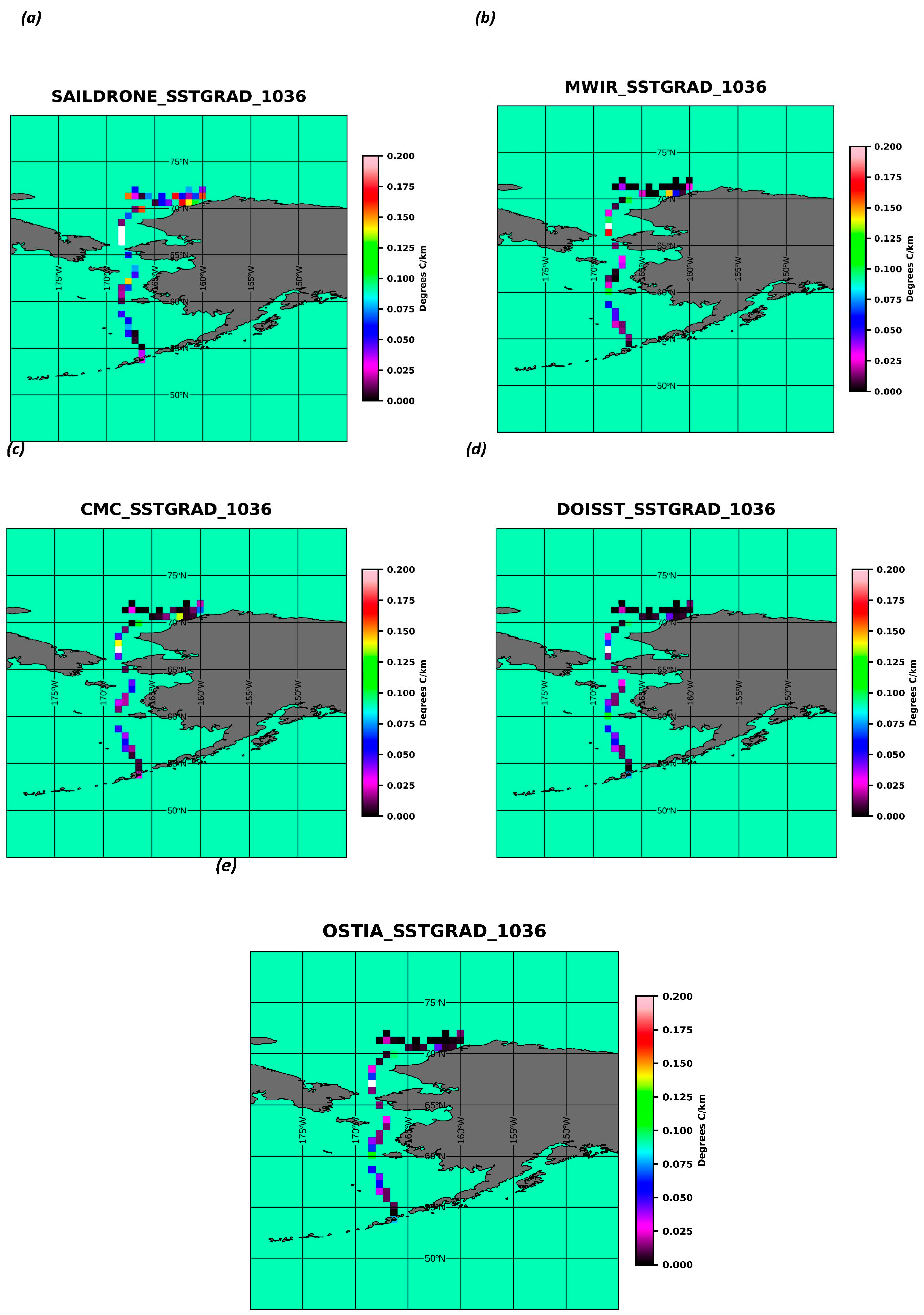
Derive SST gradients from the four satellite products based on the finite difference approach.
(4)
Collocate satellite-derived SST gradients to the daily smoothed SST gradients along the Saildrone deployment. The method used was a nearest-neighbor approach, where for a given day, the satellite-derived SST pixel closest to the Saildrone daily average for that day was chosen.
(5)
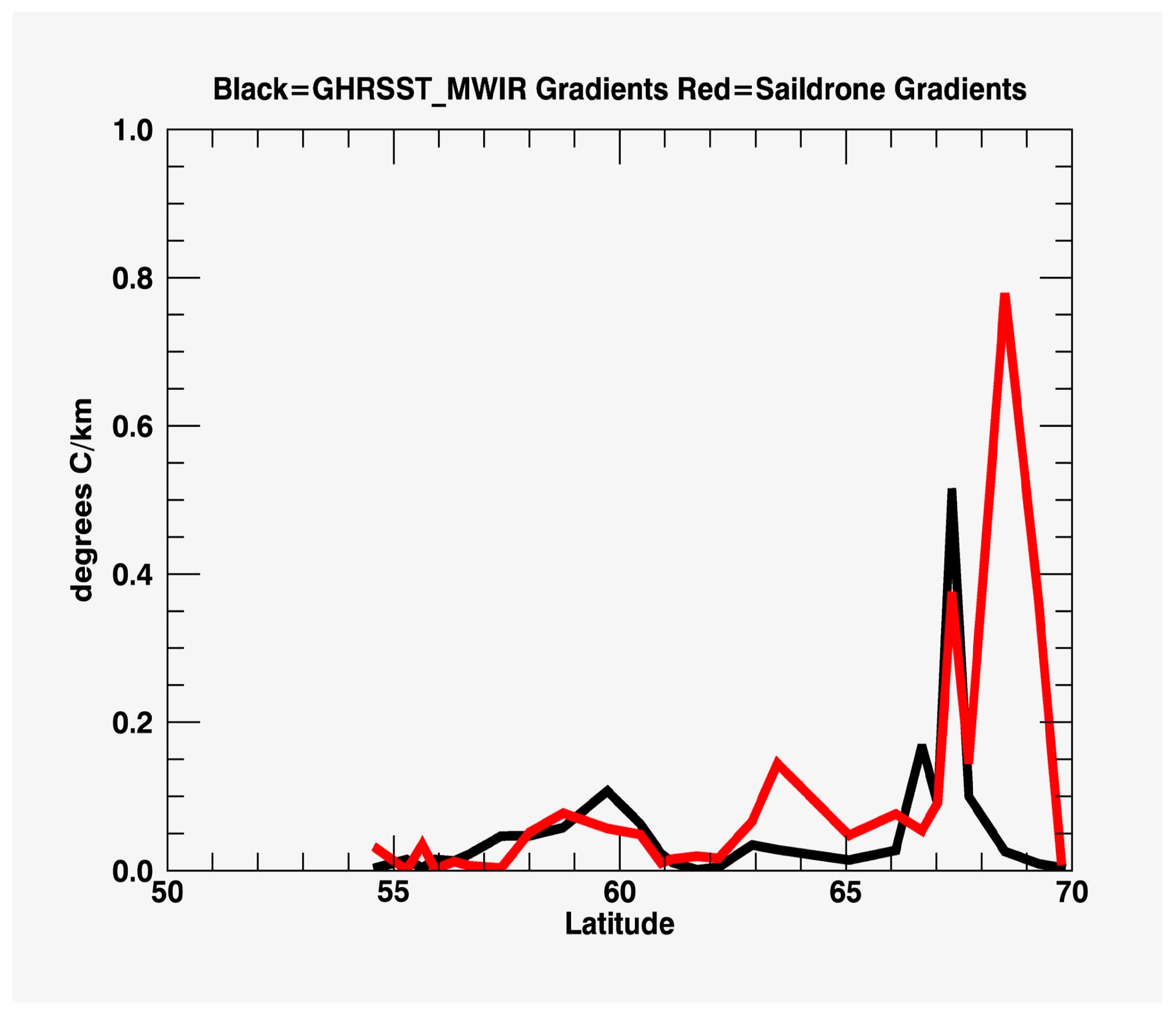
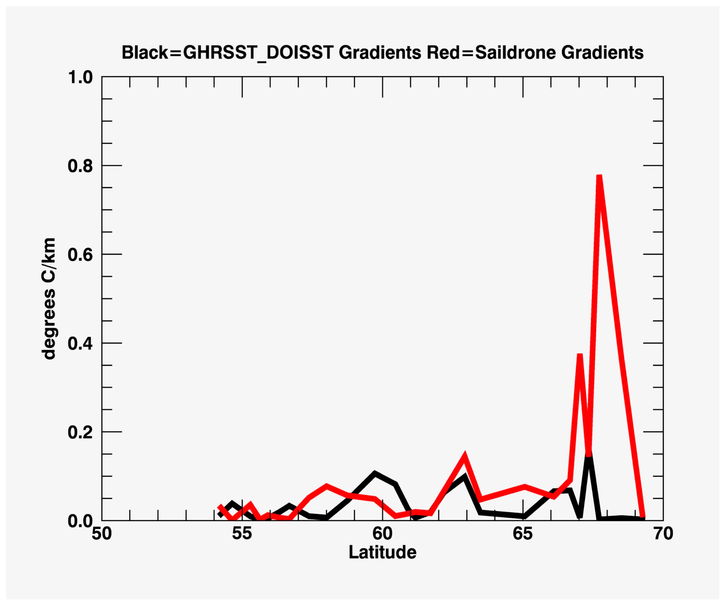
The aspatial gradients for all datasets were computed along the Saildrone track.
(6)
Linear fits were applied to the time series of the satellite-derived SST gradient maps to examine possible trends.
For step 1, the following equation was applied:
SST sail   ( x , y ) = 1 / N i N   S S T s a i l ( i )
where SSTsail (x,y) is the SST derived from the Saildrone at longitude “x” and latitude “y” after smoothing over the sub-daily time steps “N”. The index “i” simply indicates the time step along the Saildrone deployment track.
For step 2, the gradients are then derived at the daily smoothed locations along the Saildrone track.
The spatial gradients are computed, such that we have the following:
SSTsailgradx (xi,yj) = [SSTsail (xi+1,yj) − SSTsail (xi−1,y)]/Δx
SSTsailgrady (xi,yj) = [SSTsail (xi,yj+1) − SSTsail (xi,yj−1)]/Δy
where SSTsailgradx (xi,yj) and SSTsailgrady (xi,yj) are the x (longitude) and y (latitude) components of the gradient at the specified longitude and latitude locations along the Saildrone deployment track. The distances Δx and Δy are the distances in kilometers between the pixels at the specified longitude/latitude locations. The magnitude of the gradient at the location (xi,yj) along the Saildrone deployment track can then be calculated as follows:
SST sailgrad   ( x i , y j ) = S S T s a i l g r a d x ( x i , y j ) 2 + S S T s a i l g r a d y ( x i , y j ) 2
where SSTsailgrad (xi,yj) is the magnitude of Saildrone SST gradient at position (xi,yj) along the Saildrone track.
For step 3, gradients were derived for the satellite MWIR, CMC, DOISST, and OSTIA datasets for each of the daily maps covering the time period of the Saildrone deployment. The equation used is a simple finite difference approach, as follows:
SSTgradx(xi,yj) = [SST(xi+1,yj) − SST(xi−1,yj)]/Δx
SSTgrady(xi,yj) = [SST(xi,yj+1) − SST(xi,yj−1)]/Δy
The magnitude is then defined as follows:
SST sailgrad   ( x i , y j ) = S S T g r a d x ( x i , y j ) 2 + S S T g r a d y ( x i , y j ) 2
Step 4 is then defined as the collocation of values from Equation (6) with values from Equation (4).
The workflow diagram (see Figure 1) below summarizes the above steps in the methodology used for the collocation of the satellite-derived SSTs from the four products with the Saildrone deployment.
The end result consisted of collocated gradients for MWIR, CMC, DOISST, and OSTIA.
Trends of the SST gradient anomaly were derived for the satellite-derived products. The anomaly of the SST gradients was derived by removing the climatology of the satellite-derived products. Furthermore, gradient trends were derived by fitting linear least squares to the time series of the SST gradient anomaly at each satellite pixel. Four locations were also identified to exemplify regional areas where river discharge and SST gradients were identified.

3. Results

We examined the temporal behavior of SST gradients over the time period 2003–2022. SST gradients were derived for the four datasets, MWIR, CMC, DOISST, and OSTIA. Figure 2 shows the geographic study area that includes parts of the Bering Strait, the Bering Sea, and the coast of Alaska. The figure also shows the locations of the Yukon River and the discharge at the Yukon–Kuskokwim (Y-K) Delta.
The mean magnitude of SST gradients was derived for the four different products between 180°W and 165°W and 52°N and 70°N (area shown in Figure 3). To keep consistent version numbers for the products, the mean for MWIR was derived from 2003 to 2022, for CMC from 2003 to 2016, for DOISST from 2003 to 2019, and for OSTIA from 2007 to 2022. Large gradients off the western Alaskan coast for all four products are clearly visible, with values up to 0.05 °C/km, which are, nonetheless, significantly lower than the values of 0.3 °C/km found off the California coast in [14]. This is most likely because the California observations occurred during a major upwelling period, which cooled the waters near the coast. The MWIR shows the largest gradients associated with coastal regions, including the Y-K delta. A significant difference between the MWIR gradients and those from other products involves regional maxima that appear to be associated with coastal dynamics. The DOISST clearly shows the smoothest gradients. These results are consistent with the lower spatial resolution of the DOISST product. It is clear that major differences exist at latitudes greater than 65°N, where differences in sea ice become more pronounced. A common ice mask is not implemented in all the datasets and, thus, differences between the datasets could be due to the application of different ice masks. A detailed study of the ice masks is beyond the scope of this paper but should be the focus of future work in the region.
Figure 4a shows the magnitude of the SST gradients derived directly from the Saildrone data. Gradients reach maxima of 0.1 °C/km, notably near the Y-K delta and at the northern latitudes west of Alaska. Figure 4b shows MWIR SST gradients along the Saildrone deployment track, where the maxima also reach 0.1 °C/km, although no large gradients are evident in the northernmost latitudes at approximately 70°N. This is also true for the other products (CMC—Figure 4c, DOISST—Figure 4d, and OSTIA—Figure 4e). Along the Saildrone track, all the satellite products show similar magnitudes for the SST gradients except at the northernmost latitudes. Scatter plots with a more detailed explanation may be found in Appendix A.
Figure 5a–d show SICs for three dates during the Saildrone deployment. Figure 5d also shows the time series of the mean SIC for the study area between 2003 and 2022. Figure 5a is for 1 January 2019, when there was substantial sea ice north of 70°N. Pixels with significant sea ice coverage are also seen along the Alaskan Coast. Figure 5b is for 14 May 2019. The major difference from 1 January is that a significant portion of northern Alaska is now ice-free. This is an area that was sampled by the Saildrone deployment. Additionally, sea ice along the coastal areas has also disappeared. October 11 shows relatively ice-free areas north of 70°N, although ice appears around 65°N near the coast. The results indicate that sea ice is a factor in the region during the Saildrone deployment, especially along the northern Alaskan coast. It could also be a contributing factor to the large differences seen between Saildrone and the four satellite products north of 70°N. Figure 5d indicates that there is interannual variability in SIC. Note here that most GHRSST datasets refer to the areal coverage of sea ice as “sea ice fraction”, but here we refer to this as SIC to be consistent with the sea ice literature. The relationship between SST and SIC gradients will be examined further in Section 4.
Figure 6, Figure 7, Figure 8 and Figure 9 show SST gradient magnitudes from the four satellite-derived products compared with Saildrone-derived SST gradients. Figure 6 directly compares with the MWIR product. Overall, there is good agreement until approximately > 68°N, where Figure 5 indicates a large SIC at this time. The large gradients seen between 67°N and 68°N are resolved in both the Saildrone and MWIR SSTs. Figure 7 shows similar results for the CMC product, although CMC appears to also pick up the large maxima at approximately 67°N. The Saildrone SST gradient reaches 0.8 °C/km, which is considerably larger than gradients associated with mesoscale and sub-mesoscale fronts due to current instabilities and upwellings [15]. This is more evidence that these fronts are more likely associated with SST changes near ice edges. Figure 8 shows that DOISST reproduces the magnitude of the SST gradients until about 67°N, which is once again consistent with MWIR and CMC, although it fails to resolve the large gradients seen in the Saildrone SST at latitudes > 67°N. Figure 9 shows that OSTIA follows the general trend of the other products, but it best captures the magnitude of the maxima seen in the SST gradient at approximately 67°N. On the other hand, between 61–65°N, the OSTIA product overall underestimates the magnitude of the SST gradients (as do the other SST products). These latitudes are associated with river runoff, including the Y-K delta.
Table 1 compares the four different satellite products and Saildrone, using mean instead of median values in order to preserve the influence of extreme values that might arise from rapid events such as sea ice melt or river discharge (see Figure 10). The signal-to-noise ratio was defined as the standard deviation (STD) of the Saildrone-derived SST divided by the root mean square difference (RMSD) of the Saildrone SST—satellite-derived SST. The CMC and OSTIA had the highest correlation, driven primarily by the ability to resolve gradients at >67°N. DOISST had the lowest correlation, likely owing to an inability to resolve gradients at the northernmost latitude due to a low-resolution ice mask. Figure 4a clearly shows large SST gradients associated with the Saildrone, which are significantly reduced in the MWIR, CMC, DOISST, and OSTIA products. OSTIA had the highest signal-to-noise ratio, while DOISST had the lowest. This reflects the smoothness and resolution of the products, with the resolution of DOISST gridded at 0.25° and OSTIA at a resolution of 0.05°. OSTIA also had the smallest bias at −0.01 °C/km. Although MWIR had a lower correlation (0.31) and signal-to-noise ratio than DOISST and CMC, this was driven primarily by not resolving the gradient at 68–69°N. This is clearly shown in Figure 3 where MWIR shows much larger SST gradients than the other products. It is important to note that the products apply different ice masks which of course in this region will impact the evaluation of the SST gradients. For information purposes, Table 2 lists the source of the ice mask used in the particular product. The EUMETSAT product was used for both the MWIR and OSTIA products.
Figure 11a–c show multi-year linear trends of SST gradient anomalies for MWIR, CMC, DOISST, and OSTIA for the periods of time of coverage of the data. SST gradient anomalies are defined in Section 2.2. Strong trends near coastal areas are evident in all datasets. A negative trend is observed at approximately 60°N. Maximum trend values reach ~0.36 °C/km/year. Generally, OSTIA shows trends of the greatest magnitude, possibly owing to a higher signal-to-noise ratio. Figure 10 clearly shows a significant seasonal cycle in river discharge. Thus, changes in these river discharge cycles would definitely impact possible trends in SST gradients. A detailed analysis of these issues is beyond the scope of this paper but should be the focus of future work.
To examine possible connections between SST gradient anomaly trends and the Pacific Decadal Oscillation (PDO; [16] and https://www.ncei.noaa.gov/access/monitoring/pdo/), we examined three time periods using MWIR, because it extends back to 2003. The time periods chosen were 2003–2007 (negative PDO), 2008–2014 (positive PDO), and 2015–2022 (negative PDO). Large positive trends are evident in the first time period in the Bering Strait and near the Alaskan Coast. During the second time period, negative trends appear near the coast, while positive trends still appear in areas associated with coastal regions. A major difference is the appearance of negative SST gradients just north of 55°N. In the third time period, negative trends in gradients appear along the Alaskan Coast. Strong negative trends in SST gradient anomalies also appear between 55°N and 60°N. Overall, the three time periods show significant differences with trends going from positive to negative along the Alaskan Coast. Overall, the changes in the trends indicate that changes in the region are most likely occurring in steps and not necessarily in a linear fashion. These will be examined further in the next section with respect to relationships to SIC.
Four different locations in the study area (A, B, C, and D) in Figure 12 and Figure 13 were chosen as areas of special interest, e.g., location A near the winter ice edge, locations B and C near the summer ice edge, and location D near the Y-K delta. Figure 13, Figure 14, Figure 15 and Figure 16 show that, overall, DOISST has the lowest SST gradient magnitudes, while MWIR and OSTIA have the largest, with values greater than 0.3 °C/km. No clear long-term trends at the four locations are apparent. Some of the largest magnitudes are seen in location C, which is located off the North Siberian Coast. A peak occurred in the OSTIA gradients in 2004 that reached almost 0.6 °C/km. At position A, MWIR and OSTIA appear to show significant peaks past 2015. This will be examined further in the next section.
The primary goal of these results was to focus on the different magnitudes of the SST gradients for each product. The reduced magnitudes of the DOISST product are most likely due to the inherent smoothness and lower resolution of the product. The DOISST product only uses AVHRR data. The lack of microwave data will lead to gaps due to the cloud cover, which is interpolated across space and time. OSTIA and MWIR contain infrared and microwave data, while OSTIA additionally uses SST from geostationary platforms. The application of different ice masks (see Table 2) could also impact the derivation of SST gradients. A detailed analysis is beyond the scope of this paper but should be considered for future work. We note that these plots indicate SST gradient changes that do not occur linearly but in steps. The SST gradients at location A appear to have increased in variability past 2015. The possible association with changes in the southern ice edge will be examined further in the next section.

4. Discussion

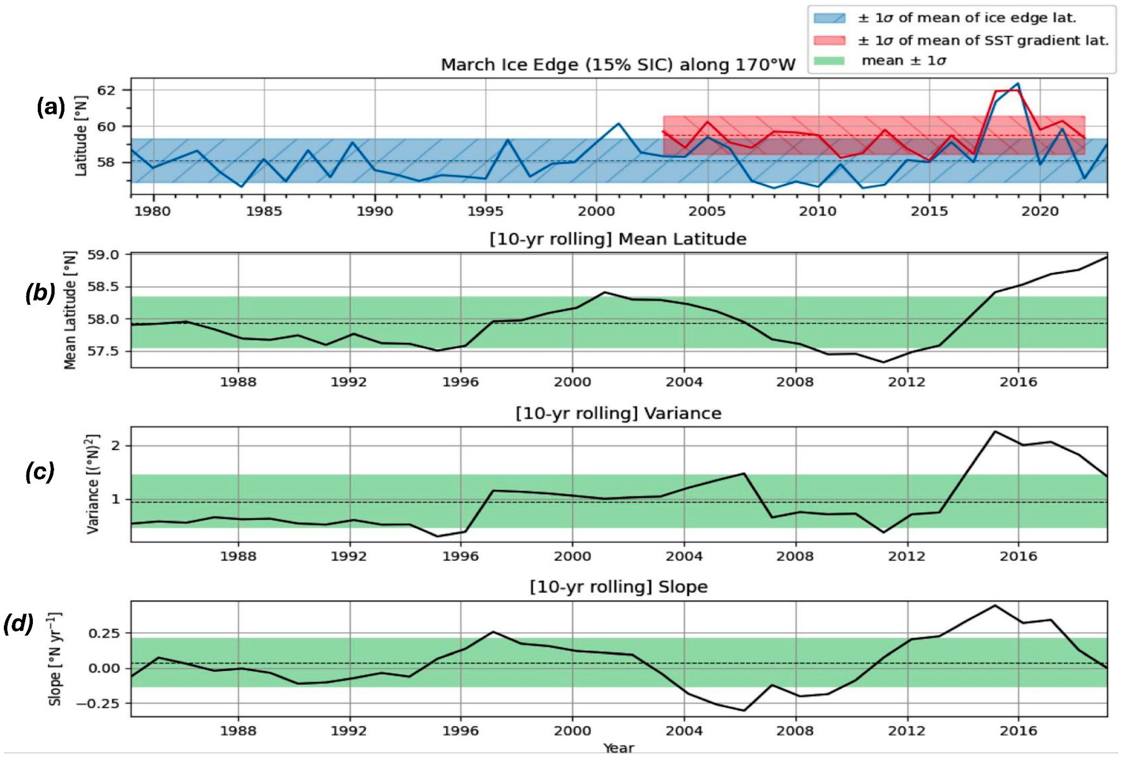
4.1. SST Gradients and Trends

Comparisons of the magnitude of the SST gradient anomalies from Saildrone 1036 with four GHRSST SST products (MWIR, CMC, DOISST, and OSTIA) indicate that, overall, the satellite-derived products do a good job at reproducing SST gradients off the Alaskan Coast. However, differences do exist at latitudes > 67°N. This is most likely due to the products applying different ice masks. OSTIA had the overall largest variability along the Saildrone track of 0.17 °C/km, with much of this driven by a large gradient at a latitude of 67°N (Figure 9). MWIR had a comparable, but smaller variability of 0.10 °C/km along the Saildrone track. These results are consistent with the two products that have the highest spatial resolution, i.e., 5 km for OSTIA, and 9 km for MWIR. The lowest-resolution (i.e., 0.25 degree) OISST product had the lowest variability of 0.04 °C/km. However, no satellite products were able to reproduce the observed 0.19 °C/km maximum gradients of the Saildrone SST. These differences were also reflected in the signal-to-noise ratios where OSTIA had the largest signal-to-noise ratio of 1.76 and DOISST had the lowest signal-to-noise ratio of 1.11. This confirms that although the OSTIA dataset is gridded at a higher resolution (5 km) than the DOISST (25 km), it does not add significant noise to the SST derivation derived from SST gradients. An obvious conclusion is that higher-resolution SST products reproduce true SST gradient variability better than lower-resolution SST products. However, other factors may also influence these intercomparisons, e.g., ice masks, input datasets, etc.
In both the MWIR and CMC products, a negative trend appears in the magnitude of the SST gradients between 55°N to 60°N (Figure 11 and Figure 12). The negative trend in the SST gradients could indicate that differences in temperatures between the North Pacific and the Arctic are decreasing. One possibility could be related to changes in the Aleutian Low. Cheng et al. [17] observed a weakening trend in the Spring Aleutian Low in the Northwest North American region. This would bring cooler temperatures to the region and would be consistent with the weakening of the gradient between waters of the Bering Strait, the Bering Sea, and the North American Coast. The primary reason for the cooling in the Northwest North American region is the reduced warmer water being brought into the high latitudes due to a weakening of the Kuroshio Extension and the North Pacific anticyclonic circulation.
Another trend observed in the higher-resolution products is the increase in gradients near the Y-K Delta (Figure 11). Increasing gradients could be consistent with trends toward increasing river discharge since river discharge temperature is often different from the ambient ocean water near its mouth [16]. Serreze et al. [18] determined that 38 percent of the freshwater input into the Arctic is due to river discharge, so understanding the impact of Arctic river discharge on SST gradients should be a focus of future work. Finally, another force for changing SST gradients could be changing SIC gradients, which will be explored in the next section.

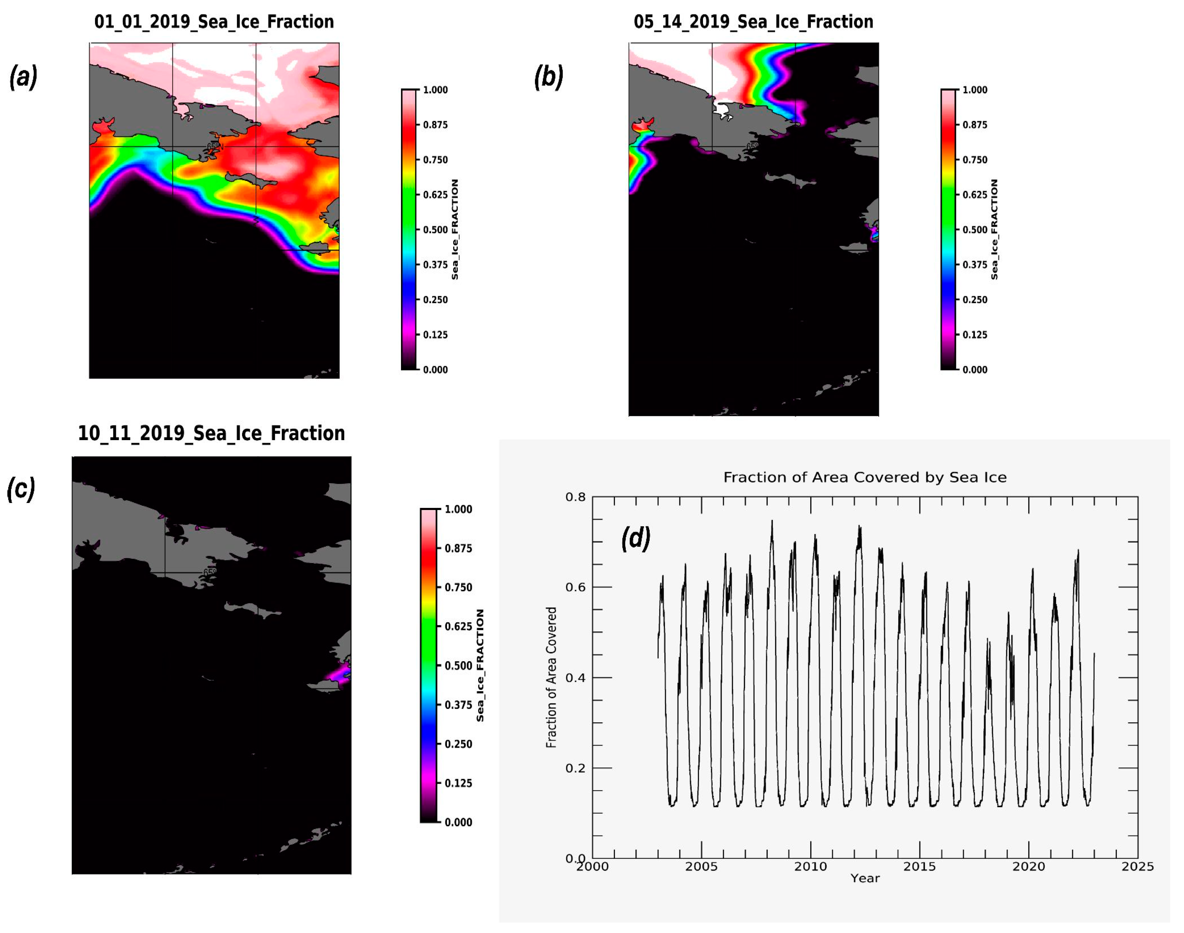
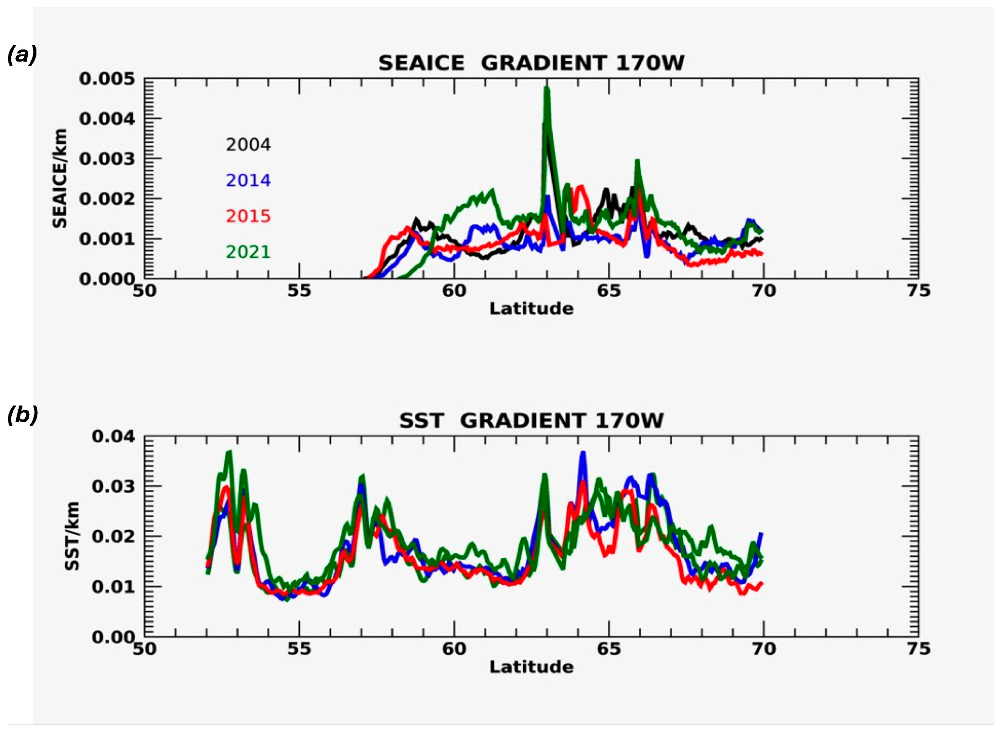
4.2. Relationship between SST and SIC Gradients

A major question that comes out of this study involves how SST and SIC gradients are related. This is also especially important in understanding how the applied ice masks impact SST gradients. Castro et al. [5] applied simulations to determine maximum SST values at the sea ice edge. In comparisons with Saildrone, they also found statistically significant correlations from several SST datasets. The goal of their work was to improve the relationship between SST and SIC, applying a filter that improved SST at ice edges.
In this work, yearly averages of SST and SIC gradients were derived for 4 years, i.e., 2004, 2014, 2015, and 2021 for our study area (Figure 17 and Figure 18). The years are representative of changes in the PDO with 2004 being neutral, 2014 and 2015 being positive, and 2021 being negative (https://www.ncei.noaa.gov/access/monitoring/pdo/). Table 3 shows statistics for the SIC and SST gradients for the four years. Overall, statistically significant correlations exist between the gradients with maxima mean gradients occurring in 2021. The strong correlations indicate a relationship exists between the SST and SIC gradients.
Moving from south to north along 170°W (Figure 19), one sees strong SST gradients at ~52–53°N at the location of the Aleutian Islands, as also seen in Figure 4. Such gradients are typical near land–sea boundaries. The next SST gradient maximum is observed at ~57–59°N, which is the position of the winter maximum (i.e., March mean) ice edge (see Figure 5). We expect strong SST gradients near the ice edge, where relatively warmer open water conditions meet the freezing water found under and near the ice pack. Next, there is a distinct SST gradient peak at 63°N and a very large SIC peak at the same location. This is where the winter polynya to the south of St. Lawrence Island forms, which tends to melt out early in the spring and summer and, thus, warm-up earlier than nearby areas that remain icy for longer. This results in strong gradients in both SIC and SST. Finally, we see strong SST gradients at 64–68°N, which are likely associated with land–sea boundaries at the Bering Strait. Figure 20 presents the same analysis for a longitude of 175°W. We see that Aleutian Island SST gradients are slightly farther south, keeping with the southwest–northeast orientation of the island chain. In contrast, the ice edge SST maximum is slightly farther north, keeping with the northwest–southeast orientation of the winter maximum ice edge in this area. Further north along this longitude, we note the absence of strong peaks in SST and SIC at 63°N that were observed at 170°W. This is likely because 175°W does not intersect St. Lawrence Island, and so does not detect the gradients associated with the Island. Finally, we see strong SST gradients around ~64.5°N to the south of the Chukotka Peninsula, then a gap through the Peninsula, and then strong SST gradients at 67.5°N on the north coast.
The interannual variation in the winter maximum (i.e., March monthly mean) ice edge (i.e., the 15% SIC contour) latitude along a longitude of 170W is shown in Figure 21, along with 10-year running mean latitude, variance, and slope. The variability is relatively small (i.e., within one standard deviation) until the year 2000, when the ice edge position moved significantly (i.e., slightly more than one standard deviation) northward for ~6 years, and after that, a comparable shift southward. After these two periods, the ice edge moved dramatically northward, achieving maximum displacement in 2018 and 2019, before shifting southward again in recent years. This analysis was also performed for January and February monthly means, which show qualitatively similar behavior (although the January ice edge position is generally a degree of latitude farther north than that in February and March). Figure 21 also shows the latitude along 170°W of the maximum SST gradient in March from OSTIA. The correlation between the two time series in Figure 21a is 0.71, indicating that a winter ice edge is a place of strong SST gradients. However, this correlation is dominated by the large northward shift in 2018 and 2019 seen in both time series. In earlier years the latitude of the SST maximum was generally 0–2 degrees north of the latitude of the ice edge, with little interannual correlation.
Throughout the entire time series, we see an increase in ice edge latitude variance, with an especially large jump in recent years. For many years, the position of the winter maximum ice edge was relatively stable (within +/−1 degree of latitude); this has changed as the ice pack has thinned and become more mobile. What does this imply for linear trends in SST gradients that are shown in Figure 11. If the ice edge position along 170°W were to shift from its traditional position at ~58°N to a more northerly position and remain there, we would expect negative SST gradient trends at the former site, and positive trends at the new site (or bands of such values all along the ice edge). However, Figure 11 shows only a band of negative trends at the traditional ice edge position. This can be explained by the enhanced recent variance in the ice edge position, which does not allow a linear trend to develop at a new, stable, more northerly position. If such variance is the “new norm” for the Bering Sea, then we should expect SST gradients associated with the winter ice edge to widely vary in position from year to year.
Overall, the northerly shift in the southern ice edge has not been a linear process but has dramatically increased over the last decade. There is also a complex relationship between SST and SIC gradients: sometimes they are spatially coincident, while in other years, there is a separation of a few degrees of latitude that might be physically real or could be the result of how the SST products fill in values under the ice. Castro et al. [5] examined this relationship in detail. Future work will need to focus on the cause of the northerly shift in the southern ice edge, with an ultimate goal of modeling and possible prediction.
The northward shift of the southern ice edge can also be related to some critical issues related to changes in the Arctic.
Ref. [20] relates Arctic amplification (AA) to sea ice loss. The results in this paper showing the northward movement of the southern ice edge indicate a possible relationship to the Arctic amplification (AA). The AA is directly related to increasing greenhouse gases. Additionally, ref. [20] states that the enhanced greenhouse warming is seen north of 67°N, which is consistent with the results found in this work and the northern movement of the southern ice edge.
Ref. [19] using model simulations showed that oceanic heat transport (OHT) through the Bering Strait had a more significant impact on Arctic warming than previously thought. A key result was also that the increased OHT was dependent on the resolution of the model. This is the motivation for further analysis of the different SST products in the Arctic. Thus, the results presented here provide a starting point for future applications of SST in the Arctic.

5. Conclusions

The validation of SST gradients derived from four GHRSST level 4 products indicates that overall satellite-derived SST gradients can be used to monitor changes in the Arctic, associated with the coast of Alaska, the Bering Strait, and the Bering Sea. Saildrone deployments provided a unique opportunity for validating SST gradients from four GHRSST products (MWIR, CMC, DOISST, and OSTIA GHRSST). OSTIA had the highest correlation and DOISST had the lowest correlation. Trends in the magnitude of the SST gradient anomalies were derived. Overall, increasing trends in the magnitude of the SST gradients were seen near the Alaskan Coast. A negative trend in the magnitude of the SST gradient anomalies was observed in a subarctic region between 55°N and 50°N. A negative trend in the region would indicate that temperatures in the subarctic and the Arctic are becoming more similar. This was also consistent with results showing a northward shift in the southern ice edge after 2018. Future work will focus on identifying the reason for the trend and possible relationships to the North Pacific circulation. Additionally, identifying changes in gradients needs to be examined with respect to changes in glacial melt. This should build on the work of [5]. This is critical as it impacts the fisheries along the Alaskan Coast. The positive results indicate that future work should expand the application of SST gradients over larger spatial scales and longer temporal scales.
A major conclusion of this work is that between 2010 and 2021, an abrupt northward shift in the winter ice edge occurred, with a coincident shift in the SST gradient. Future work needs to examine possible causes for this northward shift and possible impacts. This could include possible relationships with atmospheric forcing, river discharge, and ocean currents.

Author Contributions

J.V.-C. was involved in the conceptualization, methodology, and formal analysis of the work. Additionally, J.V.-C. wrote the initial draft. M.S. and D.S.W. supported much of the integration of the methodology to support the results. M.G.-R. and J.G.-V. were involved in the significant editing of the manuscript as well as the formal data analysis and preparation of the manuscript during the entire revision process. R.S. contributed to the editing and overall organization of the manuscript. Y.W. provided work and key results. All authors have read and agreed to the published version of the manuscript.

Funding

This research was supported through the Multi-Sensor Improved Sea Surface Temperature Project (MISST). MISST is a collaborative effort between NASA, NOAA, and the Office of Naval Research (ONR). JGV was supported by CICESE and CONAHCYT, México. MGR was funded by NASA grant nos. 80NSSC20K1003 and 80NSSC20K0768. This research was supported by NASA, through the Multi-Sensor Improved Sea Surface Temperature (MISST) project. MS and KW were funded by the MISST Project, NASA grant no. 80NSSC20K0768. M. Steele was also funded by NASA grant nos. NNX16AK43G and 80NSSC20K0134, NSF grant no. PLR 1603266, and ONR grant no. N00014-17-1-2545. DSW and JVC were also funded through NASA grant no. 80NSSC23K0643.

Data Availability Statement

All SST products used in this manuscript are available through NASA’s Physical Oceanography Distributed Active Archive Center (PO. DAAC). Information and accessibility to the products may be found at http://podaac.jpl.nasa.gov. The Saildrone data used in the analysis may also be found at https://podaac.jpl.nasa.gov/dataset/SAILDRONE_ARCTIC.

Acknowledgments

The four GHRSST SST products, along with the Saildrone deployments were downloaded from NASA’s Physical Oceanography Distributed Active Archive Center (PO.DAAC). The MWIR was downloaded from https://podaac.jpl.nasa.gov/dataset/MW_IR_OI-REMSS-L4-GLOB-v5.0. The CMC product was downloaded from https://podaac.jpl.nasa.gov/dataset/CMC0.2deg-CMC-L4-GLOB-v2.0. The DOISST product was downloaded from https://podaac.jpl.nasa.gov/dataset/AVHRR_OI-NCEI-L4-GLOB-v2.1. The OSTIA product was downloaded from https://podaac.jpl.nasa.gov/dataset/OSTIA-UKMO-L4-GLOB-v2.0. Saildrone data used in this study can also be downloaded through the PO. DAAC at https://podaac.jpl.nasa.gov/dataset/SAILDRONE_ARCTIC?ids=&values=. The research was carried out at the Jet Propulsion Laboratory, California Institute of Technology, under a contract with the National Aeronautics and Space Administration (80NM0018D0004). All the data were accessed on 10 January 2024.

Conflicts of Interest

The authors declare no conflict of interest.

Appendix A

Figure A1 shows scatter plots of SST gradients from four satellite products versus gradients measured by Saildrone; see also Table 1 for detailed statistics of this comparison. OSTIA performs best at reproducing the magnitude of Saildrone gradients, with a slope of 1.01 and a zero bias. DOISST has the smallest slope (0.45), and in particular, has trouble reproducing the largest SST gradients, likely owing to the smoothness of the product. Large SST gradients in MWIR and CMC are associated with high latitudes > 68°N and are most likely associated with issues of the ice mask. This needs to be the focus of future work. The overall statistics shown in Table 1 indicate that OSTIA performs best in comparison with Saildrone and, thus, this dataset was used for our study of the relationship between SST gradients and the winter ice edge.
Figure A1. SST gradient scatter plots for (a) MWIR versus Saildrone; (b) CMC versus Saildrone; (c) OSTIA versus Saildrone; (d) DOISST versus Saildrone.
Remotesensing 16 02530 g0a1

References

  1. Chin, T.M.; Vazquez-Cuervo, J.; Armstrong, E.M. A multi-scale high-resolution analysis of global sea surface temperature. Remote Sens. Environ. 2017, 200, 154–169. [Google Scholar] [CrossRef]
  2. Minnett, P.J.; Alvera-Azcárate, A.; Chin, T.M.; Corlett, G.K.; Gentemann, C.L.; Karagali, I.; Li, X.; Marsouin, A.; Marullo, S.; Maturi, E.; et al. Half a century of satellite remote sensing of sea-surface temperature. Remote Sens. Environ. 2019, 233, 111366. [Google Scholar] [CrossRef]
  3. Hall, S.B.; Subrahmanyam, B.; Steele, M. The Role of the Russian Shelf in Seasonal and Interannual Variability of Arctic Sea Surface Salinity and Freshwater Content. J. Geophys. Res. Oceans 2023, 128, e2022JC019247. [Google Scholar] [CrossRef]
  4. Zhang, J.; Weijer, W.; Steele, M.; Cheng, W.; Verma, T.; Veneziani, M. Labrador Sea freshening linked to Beaufort Gyre freshwater release. Nat. Commun. 2021, 12, 1229. [Google Scholar] [CrossRef] [PubMed] [PubMed Central]
  5. Castro, S.L.; Wick, G.A.; Eastwood, S.; Steele, M.A.; Tonboe, R.T. Examining the Consistency of Sea Surface Temperature and Sea Ice Concentration in Arctic Satellite Products. Remote Sens. 2023, 15, 2908. [Google Scholar] [CrossRef]
  6. Remote Sensing Systems 2017 MWIR Optimum Interpolated SST Data Set Ver. 50; P.O.D.A.A.C.: Pasadena, CA, USA, 2017. [CrossRef]
  7. Brasnett, B. The impact of satellite retrievals in a global sea-surface-temperature analysis. R. Meteorol. Soc. 2008, 134, 636. [Google Scholar] [CrossRef]
  8. Banzon, V.; Smith, T.M.; Chin, T.M.; Liu, C.; Hankins, W. A long-term record of blended satellite and in situ sea-surface temperature for climate monitoring, modeling and environmental studies. Earth Syst. Sci. Data 2016, 8, 165–176. [Google Scholar] [CrossRef]
  9. Donlon, C.J.; Martin, M.; Stark, J.; Roberts-Jones, J.; Fiedler, E.; Wimmer, W. The Operational Sea Surface Temperature and Sea Ice Analysis (OSTIA) system. Remote Sens. Environ. 2012, 116, 140–158. [Google Scholar] [CrossRef]
  10. Good, S.; Fiedler, E.; Mao, C.; Martin, M.J.; Maycock, A.; Reid, R.; Roberts-Jones, J.; Searle, T.; Waters, J.; While, J.; et al. The Current Configuration of the OSTIA System for Operational Production of Foundation Sea Surface Temperature and Ice Concentration Analyses. Remote Sens. 2020, 12, 720. [Google Scholar] [CrossRef]
  11. Gentemann, C.L.; Minnett, P.; Steele, M.; Castro, S.; Cornillon, P.; Armstrong, E.; Vazquez, J.; Tsontos, V.; Cokelet, E. 2019 Arctic Saildrone Cruise Report (Version 1); Zenodo: Geneva, Switzerland, 2019. [Google Scholar] [CrossRef]
  12. Gentemann, C.L.; Scott, J.P.; Mazzini, P.L.F.; Pianca, C.; Akella, S.; Minnett, P.J.; Cornillon, P.; Fox-Kemper, B.; Cetinic, I.; Chin, T.M.; et al. Saildrone: Adaptively sampling the marine environment. Bull. Am. Meteorol. Soc. 2020, 101, 744–762. [Google Scholar] [CrossRef]
  13. Vazquez-Cuervo, J.; Gentemann, C.; Tang, W.; Carroll, D.; Zhang, H.; Menemenlis, D.; Gomez-Valdes, J.; Bouali, M.; Steele, M. Using Saildrones to Validate Arctic Sea-Surface Salinity from the SMAP Satellite and from Ocean Models. Remote Sens. 2021, 13, 831. [Google Scholar] [CrossRef]
  14. Meier, W.N.; Fetterer, F.; Windnagel, A.K.; Stewart, J.S. NOAA/NSIDC Climate Data Record of Passive Microwave Sea Ice Concentration, Version 4; National Snow and Ice Data Center: Boulder, CO, USA, 2021. [Google Scholar]
  15. Vazquez-Cuervo, J.; García-Reyes, M.; Gómez-Valdés, J. Identification of Sea Surface Temperature and Sea Surface Salinity Fronts along the California Coast: Application Using Saildrone and Satellite Derived Products. Remote Sens. 2023, 15, 484. [Google Scholar] [CrossRef]
  16. Mantua, N.J.; Hare, S.R. The Pacific Decadal Oscillation. J. Oceanogr. 2002, 58, 35–44. [Google Scholar] [CrossRef]
  17. Sun, C.; Kucharski, F.; Li, J.; Wang, K.; Kang, I.S.; Lian, T.; Liu, T.; Ding, R.; Xie, F. Spring Aleutian Low Weakening and Surface Cooling Trend in Northwest North America During Recent Decades. J. Geophys. Res. -Atmos. 2019, 124, 12078–12092. [Google Scholar] [CrossRef]
  18. Serreze, M.C.; Barrett, A.P.; Slater, A.G.; Woodgate, R.A.; Aagaard, R.B.; Lammers, R.B.; Steele, M.; Moritz, R.; Meredith, M.; Lee, C.M. The large-scale freshwater cycle of the Arctic. J. Geophys. Res. 2002, 6, 111. [Google Scholar] [CrossRef]
  19. Xu, G.; Rencurrel, M.C.; Chang, P.; Liu, X.; Danabasoglu, G.; Yeager, S.G.; Steele, M.; Weijer, W.; Li, Y.; Rosenbloom, N.; et al. High-resolution modelling identifies the Bering Strait’s role in amplified Arctic warming. Nat. Clim. Change 2024, 14, 615. [Google Scholar] [CrossRef]
  20. Dai, A.; Luo, D.; Song, M.; Liu, J. Arctic amplification is caused by sea-ice loss under increasing CO2. Nat. Commun. 2019, 10, 121. [Google Scholar] [CrossRef]
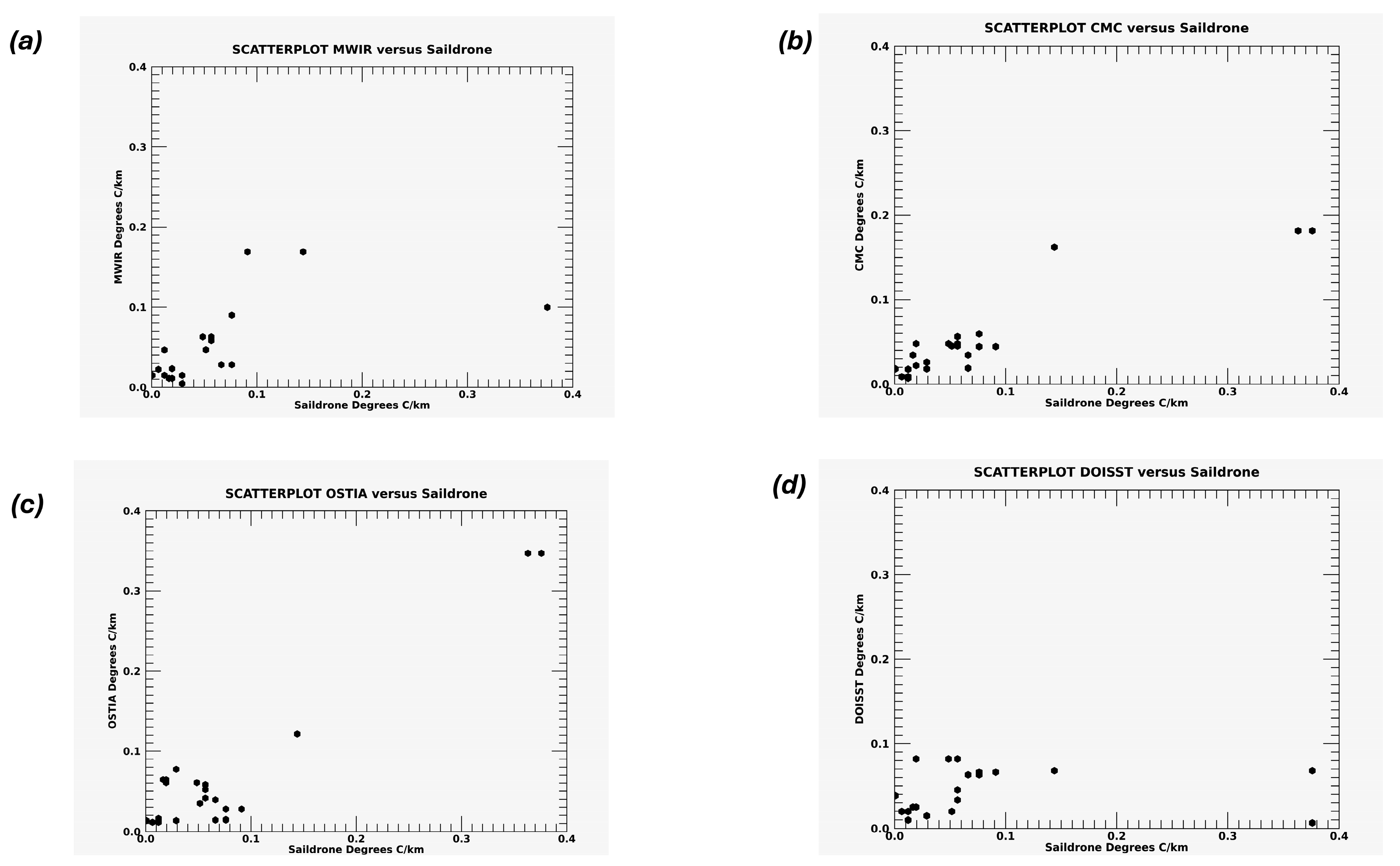
Figure 1. The workflow diagram for the derivation of SST gradients and the collocation of the SST products with the Saildrone.
Remotesensing 16 02530 g001
Figure 2. Area of study that includes the Yukon and Kuskokwim Rivers and the location of the Yukon–Kuskokwim Delta (Y-K).
Remotesensing 16 02530 g002
Figure 3. (ad): Mean SST gradient magnitude for time periods defined for (a) MWIR, (b) CMC, (c) DOISST, and (d) OSTIA.
Remotesensing 16 02530 g003aRemotesensing 16 02530 g003b
Figure 4. (ae): SST gradients along the Saildrone 1036 deployment track for (a) Saildrone deployment 1036, (b) MWIR, (c) CMC, (d) DOISST, and (e) OSTIA.
Remotesensing 16 02530 g004
Figure 5. (ad): SIF taken from OSTIA for (a) 1 January 2019, (b) 14 May 2019, (c) 11 October 2019, (d) time series of mean sea ice fraction of the area defined by Figure 4a–c from 2003 to 2022.
Remotesensing 16 02530 g005
Figure 6. The derived SST gradients versus latitude along the Saildrone 1036 deployment track and the MWIR-collocated-derived SST gradients.
Remotesensing 16 02530 g006
Figure 7. The derived SST gradients versus latitude along the Saildrone 1036 deployment track and the CMC-collocated-derived SST gradients.
Remotesensing 16 02530 g007
Figure 8. The derived SST gradients versus latitude along the Saildrone 1036 deployment track and the DOISST-collocated-derived SST gradients.
Remotesensing 16 02530 g008
Figure 9. The derived SST gradients versus latitude along the Saildrone 1036 deployment track and the OSTIA-collocated-derived SST gradients.
Remotesensing 16 02530 g009
Figure 10. River discharge for 2019. Black solid = United States Geological Survey for Yukon; red dashed = Global Flood Awareness System for Yukon; blue dashed = Anadyr River. Data were retrieved from https://waterdata.usgs.gov/ak/nwis/rt.
Remotesensing 16 02530 g010
Figure 11. (ad): The trend of the SST gradient anomaly for the defined time periods for (a) MWIR, (b) CMC, (c) DOISST, and (d) OSTIA. Labels A–D indicated locations were time series were extracted for comparisons between the data sets.
Remotesensing 16 02530 g011
Figure 12. (ac): The trend of the SST gradient for MWIR is divided into three time periods: (a) 2003–2007, (b) 2008–2014, and (c) 2015–2022.
Remotesensing 16 02530 g012
Figure 13. The time series of the maxima of the SST gradient for each year for MWIR at the 4 locations labeled in Figure 11.
Remotesensing 16 02530 g013
Figure 14. The time series of the maxima of the SST gradient for each year for CMC at the 4 locations labeled in Figure 11.
Remotesensing 16 02530 g014
Figure 15. The time series of the maxima of the SST gradient for each year for DOISST at the 4 locations labeled in Figure 11.
Remotesensing 16 02530 g015
Figure 16. The time series of the maxima of the SST gradient for each year for OSTIA at the 4 locations labeled in Figure 11.
Remotesensing 16 02530 g016
Figure 17. (ad): The mean SST gradient from OSTIA for the years (a) 2004, (b) 2014, (c) 2015, and (d) 2021.
Remotesensing 16 02530 g017
Figure 18. (ad): The mean SIC gradient for the years (a) 2004, (b) 2014, (c) 2015, and (d) 2021.
Remotesensing 16 02530 g018
Figure 19. (a,b): The top panel shows the meridional SIC gradient for years 2004, 2014, 2015, and 2021 at a longitude of 170°W for each latitude in the study area. The bottom panel shows the SST gradient.
Remotesensing 16 02530 g019
Figure 20. (a,b): Similar to Figure 19, but for 175°W. A gap in the SIC concentration exists between 65°N to 68°N, which is reflected by the straight line.
Remotesensing 16 02530 g020
Figure 21. (ad): (a) The latitude of the mean monthly March ice edge (15% SIC contour) along longitude 170°W, using the NSIDC/NOAA Climate Data Record (CDR; Meier et al. [19]) (blue). The latitude of the maximum SST gradient from OSTIA along longitude 170°W in March (red) is also shown. (b) The same as panel a for SIC, but with a 10-year running mean boxcar filter applied (and, thus, missing a few years at the start and end of the time series). Panel (c) Variance of the ice edge latitude, with the same running mean filter as in panel (b). Panel (d) same as panel (c), but for the running mean slope.
Remotesensing 16 02530 g021
Table 1. Statistics based on a comparison of MWIR, CMC, DOISST, and OSTIA with Saildrone.
DatasetCorrelationBias °C/kmRMSD °C/kmSTD Satellite °C/kmSTD Saildrone °C/kmSignal to Noise
MWIR0.31−0.040.160.100.191.17
CMC0.81−0.040.110.080.191.72
DOISST−0.11−0.060.170.040.191.11
OSTIA0.79−0.010.110.170.191.76
Table 2. Satellite products and data sources for sea ice fraction.
ProductSource
MWIRsea ice fraction (sea ice concentration) source = “EUMETSAT OSI-SAF”
CMCsea ice fraction source = “DMSP-F15 DMSP-F17 DMSP-F18 Metop-1 Metop-2 Metop-3 G COM-W1”
DOISSTsea ice fraction source = “MMAB_50KM-NCEP-ICE”
OSTIAsea ice fraction source = “EUMETSAT OSI-SAF”
Table 3. Statistics of comparisons between the SIC and SST gradients for the study region and the selected 4 years of study.
YEARCORRELATIONMEAN SIC Gradients (SIC/KM)MEAN SST Gradients (Degrees C/KM)RMS SIC Gradients SIC/KM)RMS SST Gradients (Degrees C/KM)
20040.960.00080.01750.00080.006
20140.940.00060.01730.00040.006
20150.950.00060.01590.00050.005
20210.960.00080.01850.00080.005
Disclaimer/Publisher’s Note: The statements, opinions and data contained in all publications are solely those of the individual author(s) and contributor(s) and not of MDPI and/or the editor(s). MDPI and/or the editor(s) disclaim responsibility for any injury to people or property resulting from any ideas, methods, instructions or products referred to in the content.

