Article

Characterisation of Two Vineyards in Mexico Based on Sentinel-2 and Meteorological Data

1
Department of Mathematics and Physics, Arkansas State University, Carretera Estatal 100, km 17.5, Municipio de Colón 76270, Querétaro, Mexico
2
Departamento de Física de la Tierra y Astrofísica, Universidad Complutense de Madrid (UCM), Plaza de Ciencias, 1, Ciudad Universitaria, 28040 Madrid, Spain
*
Author to whom correspondence should be addressed.
Remote Sens. 2024, 16(14), 2538; https://doi.org/10.3390/rs16142538
Submission received: 27 April 2024 / Revised: 26 June 2024 / Accepted: 6 July 2024 / Published: 10 July 2024
(This article belongs to the Special Issue Remote Sensing in Viticulture II)

Abstract

:
In Mexico, viticulture represents the second source of employment in the agricultural area after the fruit and vegetable sector. In developed countries, remote sensing is widely used for vineyard monitoring; however, this tool is barely used in the developing countries of Iberoamerica. In this research, our overall objective is to characterise two vineyards in the state of Queretaro (Mexico) using Sentinel-2 and meteorological data, specifically spectral and thermal indices. Results show that spectral indices obtained from Sentinel-2 bands have adequately characterised the phenological dynamics of the different varieties of the vineyards. The Modified Soil-Adjusted Vegetation Index (MSAVI) was adequately used to discriminate between the first stages of vineyards, while the Normalized Difference Vegetation Index (NDVI) was useful for monitoring vineyards during the rest stages of vineyards. Thermal indices have shown that the best grape varieties are those that can adapt to both cooler and warmer temperatures, have a reasonable ripening period, and can produce wines with balanced acidity and flavours. In conclusion, the combination of meteorological (including thermal indices) and remote sensing data (NDVI and MSAVI) provide information for choosing a suitable grape variety for this region.

1. Introduction

Vineyards occupied 7.21 million hectares worldwide in 2023, according to the International Organization of Vine and Wine [1]. Although viticulture is concentrated around Mediterranean countries [1,2], there are other regions in the world in which viticulture shows importance, such as Mexico, where vineyards occupy 36,000 ha and represent the second source of employment in the agricultural sector after the fruit and vegetable sector [3]. Specifically, in the state of Queretaro, viticulture is clearly in expansion, and numerous wineries have been consolidated in the last decade [4]. Grapevine health and productivity are influenced by various factors, such as topography, climate, soil characteristics, types of mechanisation, and pests and diseases. These factors create spatial and temporal variations within vineyards, leading to differences in grape quality and yield [5]. This can result, in some circumstances, in lower-quality wine and reduced volume. The wine industry needs to consider these variabilities in quality and yield to produce a higher-value product.
Remote sensing allows for continuous monitoring at different spatial and temporal scales of crops over large areas [6,7], providing valuable information on their health, growth, and overall condition, and also can be used to estimate crop yields by analysing vegetation indices and other indicators of plant health. Remote sensing information is usually summarized as spectral indices that are related to physiological processes such as photosynthesis [8,9]. The Normalized Difference Vegetation Index (NDVI) [10] is the most widely used vegetation index that quantifies the density and health of vegetation by analysing the difference between the near-infrared (NIR) and red (Red) bands. Other ratio spectral indices are the Enhanced Vegetation Index (EVI) [11] and the Modified Soil-Adjusted Vegetation Index (MSAVI) [12], which is a modification of the Soil-Adjusted Vegetation Index (SAVI) [13] and aims to reduce the sensitivity of the index to soil background effects. The MSAVI considers the vegetation and soil reflectance properties and provides a more accurate measure of vegetation density and health than other indices during the first vegetative stages. The study of vineyards through spectral indices has been widely used in the last decades [14,15,16]. Low spatial resolution sensors, such as the Moderate Resolution Imaging Spectroradiometer (MODIS), have been used to assess vineyard management by estimating growing season length through NDVI [17] or monitoring grapevine requirements through MODIS Land Surface Temperature (LST) [18]. The results of MODIS data analyses have contributed to our understanding of the Earth’s system and informed policy and management decisions [11,19]. Unmanned aerial vehicles (UAVs). and higher-resolution sensors present a new opportunity for monitoring crops in Latin America [20], such as vineyards. In this sense, recent studies have used spectral indices acquired through UAV to assess vineyard zoning in Serbia [21] and Spain [22]. On the other hand, Sentinel-2 has combined higher-resolution images (10 m) with a higher temporal resolution (5 days). There are recent and multiple applications with spectral Sentinel-2 spectral indices in vineyards, such as quantifying the impact of heatwaves [23], the damage of frosts [24], estimating actual evapotranspiration [25], and characterizing vineyards in different regions. In this sense, Devaux et al. [26] showed the ability to monitor vine growth with Sentinel-2 NDVI images in a southern region of France. Additionally, Stolarski et al. [27] used Sentinel-2 NDVI images and unmanned aerial vehicles to assess vigour management and to detect vineyard variability in two vineyards in Portugal. In addition, Vélez et al. [28] used Sentinel-2 NDVI time series to assess relevant phenological stages and agronomic parameters in the vineyards of Spain.
Remote sensing for vineyard monitoring has been widely used in developed countries; however, this tool is barely used in the developing countries of Iberoamerica [29,30]. The use of UAVs is expensive; however, the information provided by satellites, such as Sentinel-2 and Landsat, has a free access policy and their use is increasing in developing countries [31]. It is essential that these regions can access these new tools for satisfying the sustainable development goals (SDG) of the United Nations (web SDG). Goal number 2 (zero hunger) implies the use of technology for crop management to achieve this goal. In addition, goal number 9 highlights “that technological progress is a key factor to finding lasting solutions to both economic and environmental challenges” [32].
On the other hand, thermal indices, based on different temperature data, are widely used in vineyards to assess the suitability of climate conditions for grapevine growth and development and for the health level for calculating plant protection [33,34,35]. Several thermal indices have been developed specifically for viticulture, including the Winkler Index [36,37], the Huglin Index [38], the growing season temperature [33,39], and the Cold Index [40]. The Winkler Index estimates the grapevine’s heat summation during the growing season, which is the sum of the mean daily temperature above 10 °C, while the Huglin Index estimates the potential grape yield based on growing degree days (GDDs) above 10 °C during the growing season. The Growing Season Temperature (GST) Index is another important index that considers both temperature and the timing of key growth stages to provide a measure of the climate suitability for specific grapevine varieties. Finally, the Cold Index (CI) considers the number of frost-free days and the sum of GDD to estimate the suitability of a region for grapevine growth. Thermal indices provide complementary information and allow us to compare our results in Mexico with those from different parts of the world. Altogether, classifying vineyards with thermal indices can provide valuable insights for vineyard management and grape production [41,42]. This kind of information could be accompanied by remote sensing spectral indices to obtain an accurate assessment of vineyards. To the best of our knowledge, this is the first work that combines spectral indices with thermal indices and meteorological information obtained from satellites. This research, based on [43], is a more in-depth study of two vineyards in Queretaro.
In this paper, our overall objective is to characterize two vineyards in the state of Queretaro (Mexico) using Sentinel-2 and meteorological data, with the following specific objectives:
  • To assess the dynamics of the main meteorological elements of the two vineyards.
  • To assess the phenology of the two vineyards through spectral vegetation indices (NDVI and MSAVI).
  • To obtain thermal indices of the two vineyards and compare them with other wine-producing regions.
  • To relate meteorological information to spectral indices.

2. Materials and Methods
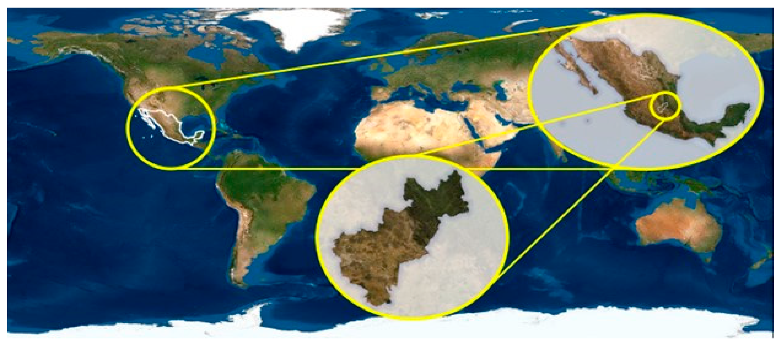
2.1. Study Area

Queretaro is a state in Mexico located between the parallels 21.7°N and 20.0°N, and specifically, the vineyards are located between 20.4°N and 20.8°N. The vineyards are completely outside of the “wine belt”, which is between latitudes 30° and 50° (Figure 1), in both hemispheres. The climate of the studied vineyards is arid, steppe, cold, and Bsk, according to the Köppen–Geiger climate classification [44]. However, the large altitude, close to 2000 m above sea level (asl), produces mild winters that allow the vine to rest. Two separate representative vineyards were selected in Queretaro State, one in the municipality of El Marques (22.7 ha), Puerta del Lobo, henceforth PL, and the other in the municipality of Colon (23.8 ha), Vinaltura, henceforth VA (Figure 2). These two vineyards were selected first for their location in two different municipalities, second for their size; they are among the largest in the region, third because they both have weather stations, and finally, they are the ones where we had access to the variety planted by plot, which allowed studying the relationship between vegetation indices and the phenology of the vines. The predominant soil (more than 60%) in both vineyards is vertisol, with areas of leptosols and phaeozems in PL, and the texture is clay-loam. Vertisols are very heavy clay soils with a high proportion of swelling clays.
The physical characteristics of vineyards play a crucial role in determining the quality and yield of grapes. Table 1 summarizes the key physical characteristics of both vineyards, revealing striking similarities in their extension, precipitation, slope, temperature, and other factors. These similarities are not surprising given that vineyards require specific climatic conditions to flourish, and both are located relatively close (~24 km). As it is observed in Table 1, the average annual temperature for 2022 in both vineyards (PL-18.5 °C and VA-18.5 °C) was 1 °C higher than the average annual temperature of the period 1981–2023 (PL-17.6 °C and VA-17.5 °C). Figure 3 shows the average maximum and minimum monthly temperatures and monthly rainfall for 2022 and for the period 1981–2023. It can be remarked that in both vineyards, the maximum temperatures in May and July of 2022 were higher than in the average period, while in September the maximum temperature was slightly lower. Meanwhile, the annual precipitation was much lower for the year 2022 in both vineyards (PL-353.64 mm and VA-315.42 mm) than for the period 1981–2023 (PL-521. 4 mm and VA-472.5 mm), this year being especially dry. Figure 3 shows the significantly lower amount of precipitation in May, June, and July of 2022 than for that period.

2.2. Phenological Stages

Table 2 shows the average data for all the varieties of the main phenological stages recollected in the field by the winegrowers in the two vineyards. This data will be compared to the phenological stages observed by remote sensing data in results section.

2.3. Remote Sensing and Reanalysis Data

The images used to calculate spectral or vegetation indices (NDVI and MSAVI) are from Sentinel-2, downloaded through Google Earth Engine. The Sentinel-2 mission is part of the Copernicus program, which has been developed and is operated by the European Space Agency (ESA) [45]. The mission relies on a constellation of two identical satellites that provide images with a high spatial (10 m, 20 m, and 60 m) and temporal resolution (5 days).
In this research, Level-2A bottom-of-atmosphere (BOA) images of 10 m were used, which means these images are already atmospheric and topographically corrected from the top-of-atmosphere (TOA) level-1C orthoimage products.
Apart from Sentinel-2, images from the Shuttle Radar Topography Mission (SRTM) [46] were used to calculate the altitude and slope/inclination of the vineyards. Temperatures to calculate the thermal indices were obtained from ERA-5 Land, a reanalysis dataset (spatial resolution ≈ 11 km) produced by Copernicus Climate Data Store [47] and DAYMET-V4 (spatial resolution ≈ 1 km) [48]. The Climate Hazards Group InfraRed Precipitation with Station data (CHIRPS) was used for calculating precipitation (spatial resolution ≈ 5.5 km) to compare with data from the meteorological stations [49].

2.4. Meteorological Data from Automatic Weather Stations (AWSs)

Meteorological information obtained from the Davis Vantage Pro 2 station is of great importance to vineyards. The station can monitor the meteorological conditions of vineyards, including temperature, relative humidity, precipitation, wind, and solar radiation. These meteorological variables affect the growth and development of grapes and, therefore, play a crucial role in the quality and yield of the final wine product. For instance, temperature and humidity influence the ripening process of grapes, while wind and precipitation can damage grapevines and affect the yield.

2.5. Methods

Biweekly Sentinel-2 MSI Level-2A composite images from January 2022 to December 2022 were used, with a maximum cloud cover of 5% in each tile, which, in all cases, resulted in cloud-free images for the studied area, except for the second half of August and the first half of September, when cloudiness was much higher in these areas, and we used 50% maximum coverage to better cancel cloud or clouds’ shadows by calculating the median image. The software used to analyse the data was QGIS 3.22, Google Earth Engine, and Python 3.12.

2.5.1. Spectral Indices

Normalized Difference Vegetation Index (NDVI)

The NDVI [10] ranges from −1 to 1 (Equation (1)), with higher values indicating more dense and healthy vegetation. Table 3 shows the interpretation of the values [50].
NDVI is a useful tool for vineyards to monitor vegetation health and vigour. NDVI values can be used to estimate the amount of photosynthetically active biomass in the vineyard, which is a critical factor in grapevine growth and productivity. By monitoring NDVI values over time, vineyard managers can track changes in vineyard health and identify areas that may require additional irrigation or nutrient management. The NDVI can also be used to map the vineyard and identify areas of stress or variation in growth, which can be used to make informed decisions about planting, pruning, and harvesting. In short, the NDVI is a valuable tool for vineyard management, allowing for efficient and effective monitoring of vineyard health and productivity [51,52].
For Sentinel-2, this index is defined as Equation (1):
N D V I = N I R + R e d N I R R e d = B 8 B 4 B 8 + B 4  
where B8 is the NIR band and B4 is the Red band in Sentinel 2.

Modified Soil-Adjusted Vegetation Index (MSAVI)

The Modified Soil-Adjusted Vegetation Index (MSAVI) [12] (Equation (2)) considers the vegetation and soil reflectance properties and provides a more accurate measure of vegetation density and health than other indices (Table 4, [50]). It is commonly used in remote sensing applications to monitor vegetation growth, drought stress, and other environmental changes during seed germination and leaf development stages. The MSAVI is effective in a variety of vegetation types, including forests, croplands, and grasslands. In general, the MSAVI is a valuable tool for assessing vegetation health and monitoring changes in vegetation density over time [53,54].
For Sentinel-2, this index is defined as:
M S A V I = 2 N I R + 1 2 N I R + 1 2 8 N I R R e d   2   = 2 B 8 + 1 2 B 8 + 1 2 8 B 8 B 4   2                
where B8 is the NIR band and B4 is the Red band in Sentinel 2.

2.5.2. Thermal Indices

Thermal indices were calculated with data taken every 30 min from the weather stations for the year 2022. These results were compared when it was possible from catalogue images of ERA5-Land (Copernicus Climate Data Store [47]) and NASA DAYMET catalogue [48]. In addition, due to the climate variability of the area, the different average climate indices for the period 2000–2022 [43] were compared with our results.

Winkler Index (WI)

The Winkler Index (WI), also referred to as the Winkler Scale or Winkler Regions, first proposed by Amerine and Winkler [36] and later modified by Winkler [37], is a method of categorizing wine-growing regions based on the accumulation of heat or growing degree days (Equation (3)). The technique divides geographical areas into five climate regions, labelled as Regions I to V, based on the temperature that is converted to growing degree days.
    W I = April   1 October   31 ( T mean 10   ° C )      
This index determines the suitability of crop growth in different climates. Region I (cold) produces table wines, light-moderate and with good balance, with only early-ripening varieties achieving high quality; Region II (temperate), early and mid-season table wine varieties, will produce good-quality wines; Region III (temperate-warm) produces dry and sweet table wines and light dessert wines, and is favourable for high production of standard- to good-quality table wines; Region IV (warm) is favourable for high production, but acceptable table wine quality, at best; and Region V (very warm) is typically only suitable for extremely high production, fair-quality table wine or table grape varieties destined for early-season consumption.
Examples of Region I are Champagne and Burgundy (France), Rhine Valley (Germany), and Ribera del Duero (Spain). Examples of Region II are Piedmont (Italy), Anjou (France), and Rioja (Spain). Region III is well represented by Rueda and Priorat (Spain), Sonoma Valley (California), Bordeaux (France), and Chianti and Toscana (Italy). In Region IV, we have Napa Valley (California), Tuscany (Italy), and Reus (Spain). Finally, examples of Region V are Madeira (Portugal), Patras (Greece), and Jerez (Spain).

Huglin Index (HI)

The Huglin Heat Sum Index (HI) is a bioclimatic heat index developed by Huglin [38] for vineyards. It calculates the temperature sum over a threshold of 10 °C by summing the average daily and maximum temperatures for all days from the beginning of April to the end of September (Equation (4)). The calculated total is slightly modified based on the latitude of the area (factor K). The value of K is tabulated for latitudes between 50° and 40°; below this latitude, K = 1 is used, which is the value we have taken [41]. The HI is used to determine the suitability of an area for cultivating different grape varieties over the long term, as each variety requires a specific amount of heat for successful cultivation.
  H I = K April   1 Sept   30 T mean + T max 2 10 ° C    

Cold Nights Index (CI)

The Cold Night Index (CI) is a viticultural climate index developed by Tonietto [40] and Tonietto and Carbonneau [41] to estimate the microthermal condition during the grape maturation period. The index utilizes minimum temperatures (Equation (5)) as an indicator of the region’s potential characteristics related to secondary metabolites, such as polyphenols, aromas, and colour, in grapes and wines [55].
The Cold Night Index is a variable that considers the average minimum night temperatures during the ripening month, extending beyond the ripening period.
    C I = Sept   1 Sept   30 T min 30  

Growing Season Temperature

The growing season temperature (GST) index is a metric used in viticulture to assess the suitability of a specific region for wine production [33,39]. It considers the temperature conditions during the growing season (1 April to 31 October), which are crucial for grape development and ripening (Equation (6)).
The index typically involves calculating the sum of the average daily temperatures during the growing season, which allows for an estimation of the accumulated heat units or degree-days experienced by the grapevines. This information is important for determining grape phenology, such as bud break, flowering, veraison (colour change of grapes), and harvest time.
The GST index indicates the daily mean temperature between 1 April and 31 October in the Northern Hemisphere. This index broadly correlates with the maturity potential of winegrape cultivars.
  G S T = April   1 October   31 T mean n  

2.6. Statistical Analysis

The relationship between vegetation indices and the phenology of the vines has been calculated by comparing our maps (see Section 3.2) with the data collected in the field.
The relationship between NDVI and precipitation (Section 3.3) has been assessed through the Pearson correlation coefficient [56]:
r = i x i x ¯ y i y ¯ i x i x ¯ 2 i y i y ¯ 2       .
However, it is noted that the coefficient ‘ r ’ alone may not robustly determine the statistical significance of observed correlations or the comparative strength between correlations. To substantiate our findings, we employed the complementary error function (erfc) defined as follows [56]:
e r f c = r N 2       .
A diminutive value of Equation (8) signifies a significant correlation between the two distributions.

3. Results

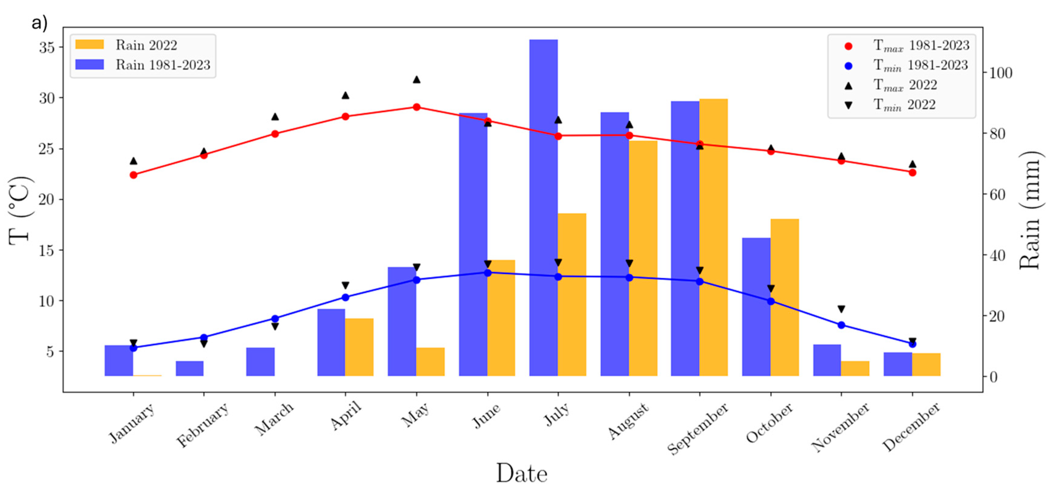
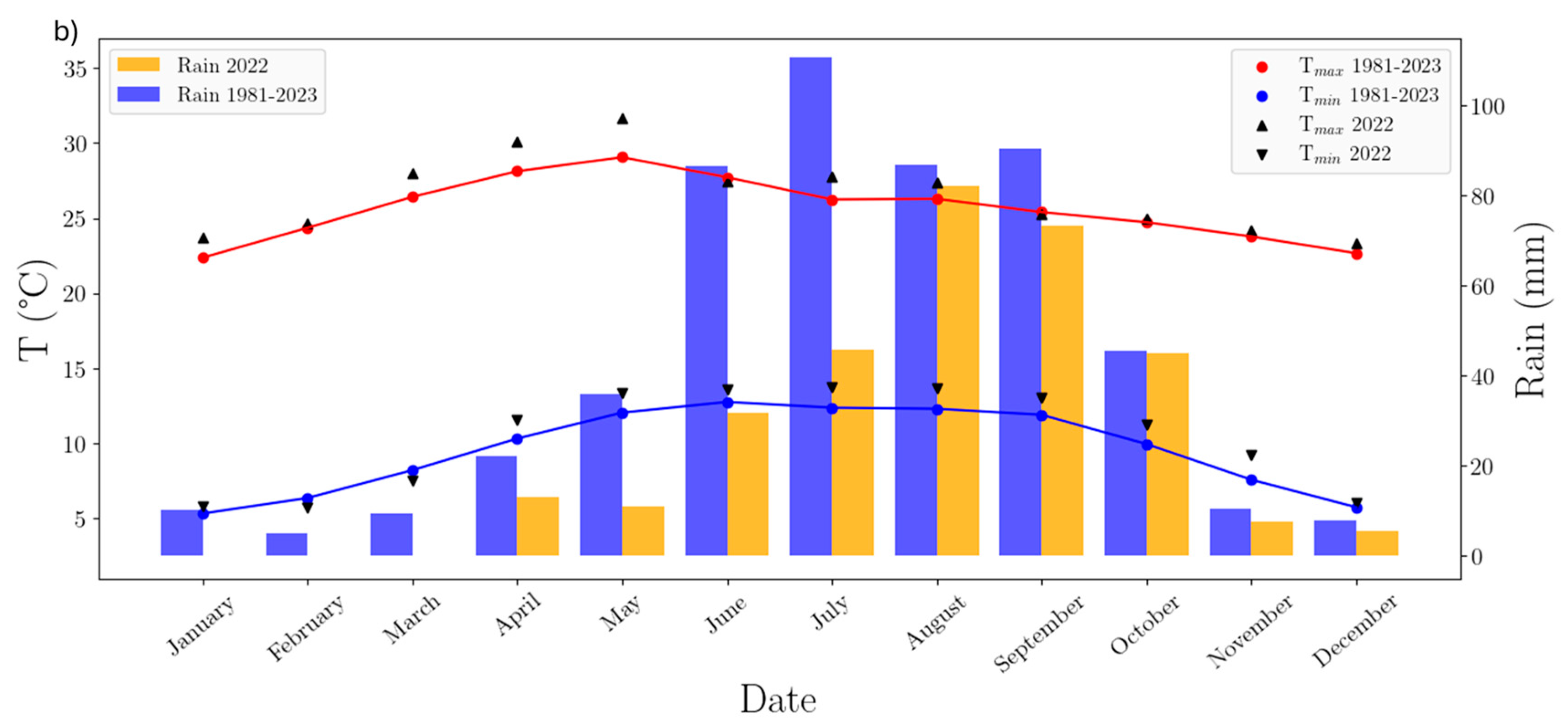
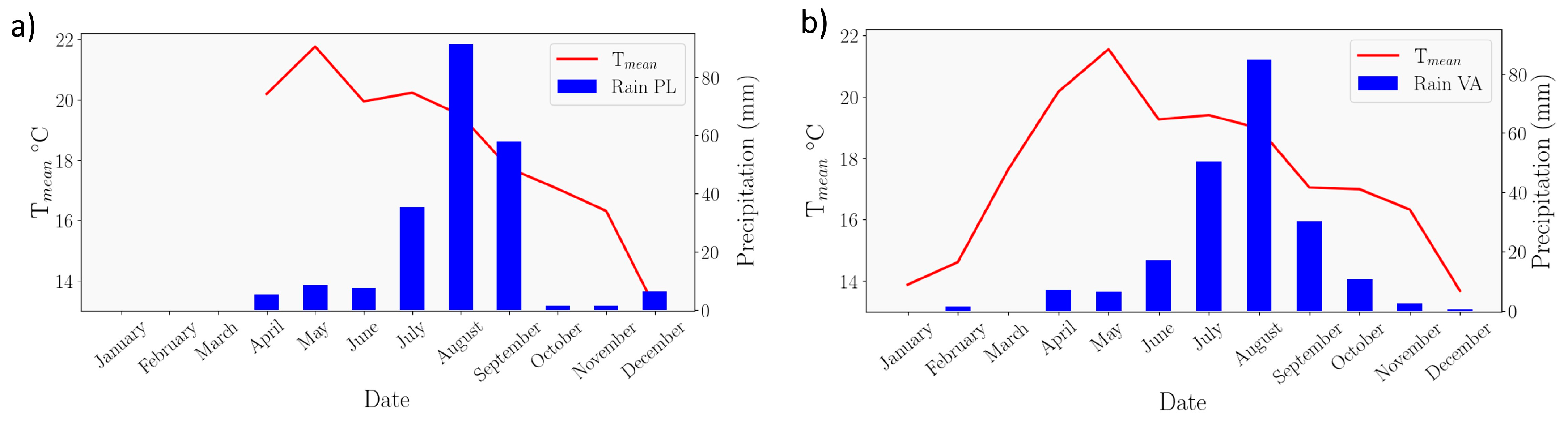
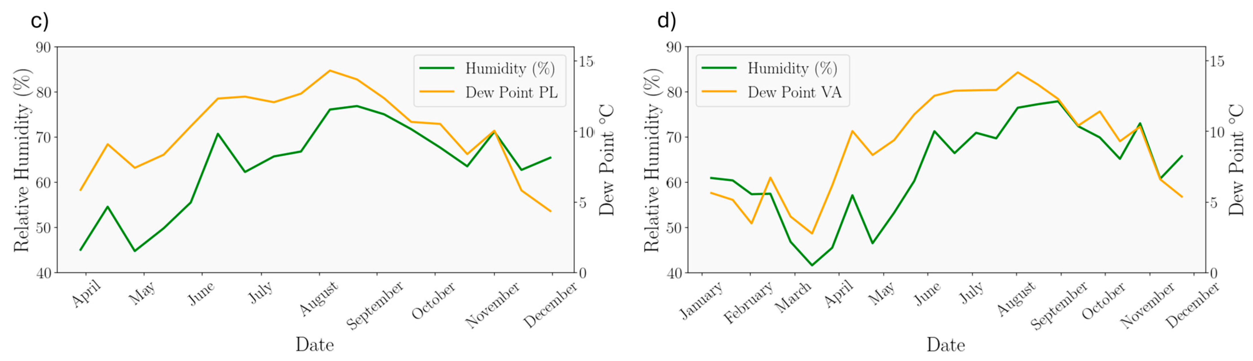
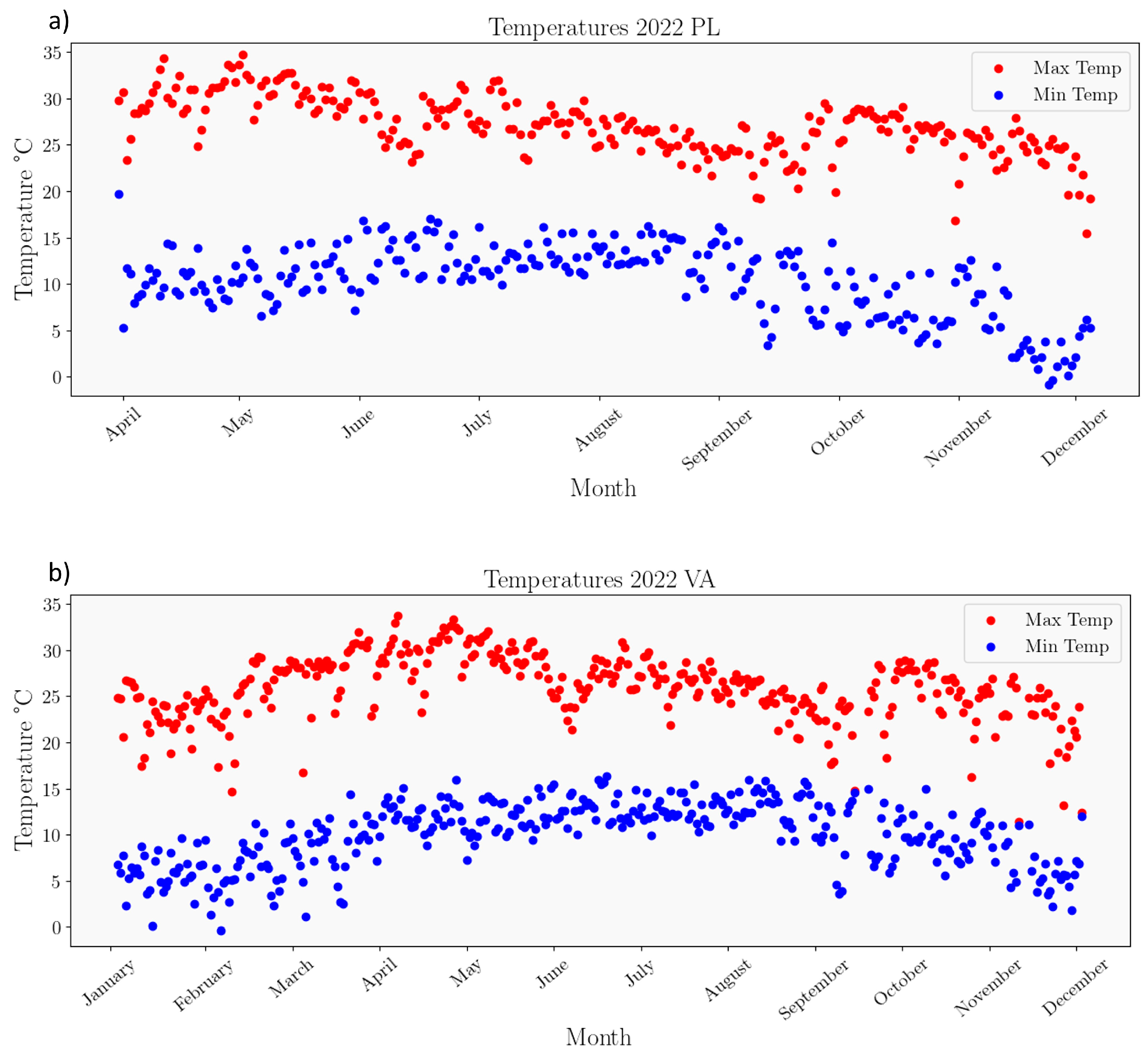
3.1. Dynamics of Meteorological Elements of the Vineyards

Figure 4 shows the dynamics of temperature (°C), precipitation (mm), relative humidity (%), and dew point (°C) during the year 2022 in the two vineyards, according to the meteorological stations. As it can be observed, in PL, there was no data from January to March.
The monthly temperature was minimal during January (14 °C), then increased until May, reaching a maximum of around 21 °C. After May, the monthly temperature decreased approximately steadily until December, when minimum values were reached again.
In this type of climate, the rainy season lasts around 4 months between June and September. Precipitation levels showed their monthly maximum values in August and their minimum values between December and March.
The dynamics of relative humidity and dew point depend strongly on the precipitation and temperature dynamics as well as on the phenology of the vineyards. Both variables showed their minimum in January, and then they increased during the following months with the increase in temperature and especially with the availability of water. Relative humidity reached its maximum in summer due to the high precipitation and the evapotranspiration, which was maximal due to the full development of the vineyards, in addition to the water content accumulated in the soil due to precipitation of the preceding months, although temperature was also high in summer, which could entail a reduction in relative humidity.
Figure 5 shows the dynamics of the daily maximum and minimum temperatures at both sites. In PL, the maximum temperature ranges between 17 °C in December and 35 °C in May, while the minimum temperature ranges between 0 °C in December and 16 °C in June. In VA, temperatures are slightly lower, with the maximum temperature ranging between 11 °C in December and 34 °C in May and the minimum temperature ranging between −1 °C in January and 15 °C in July.

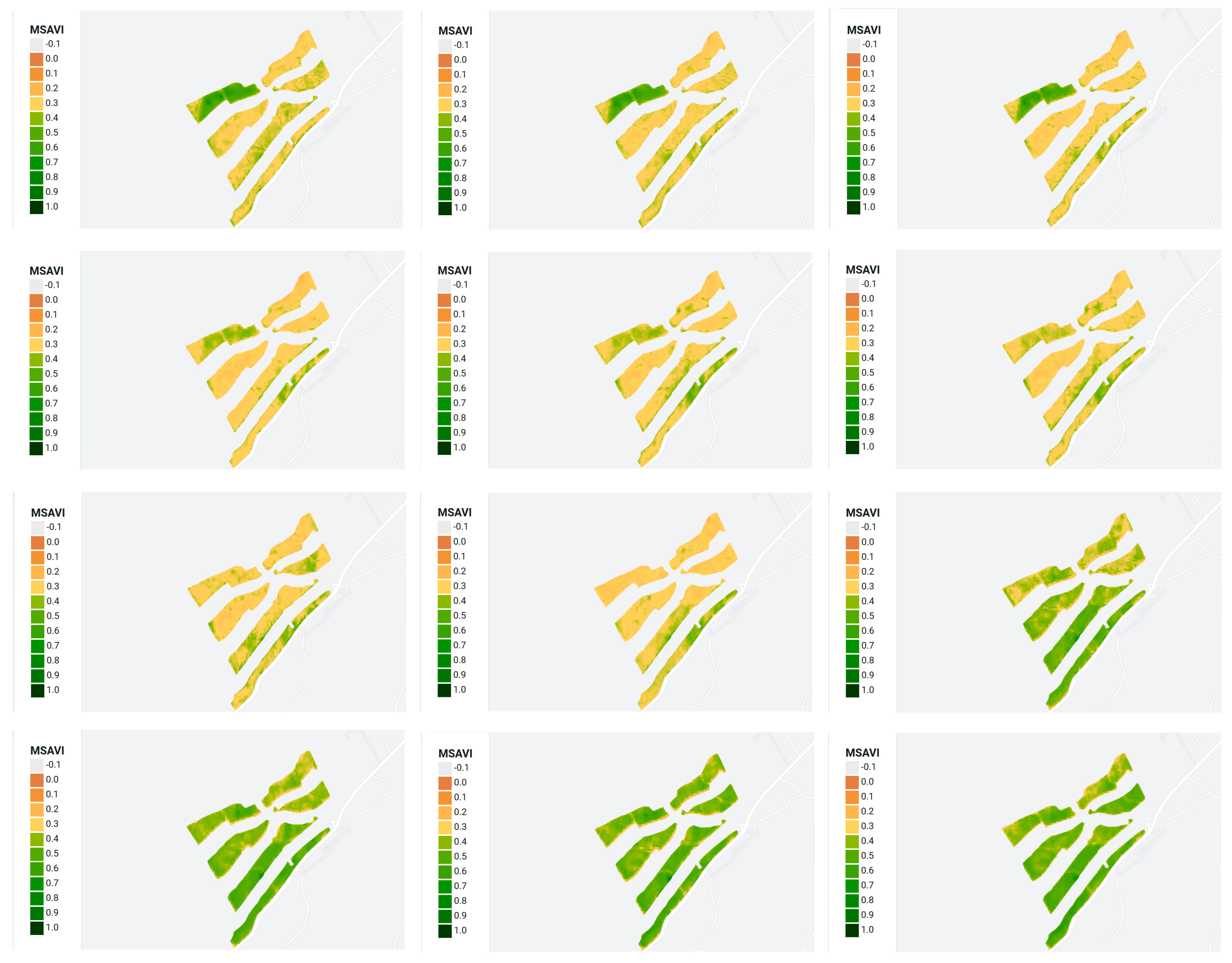
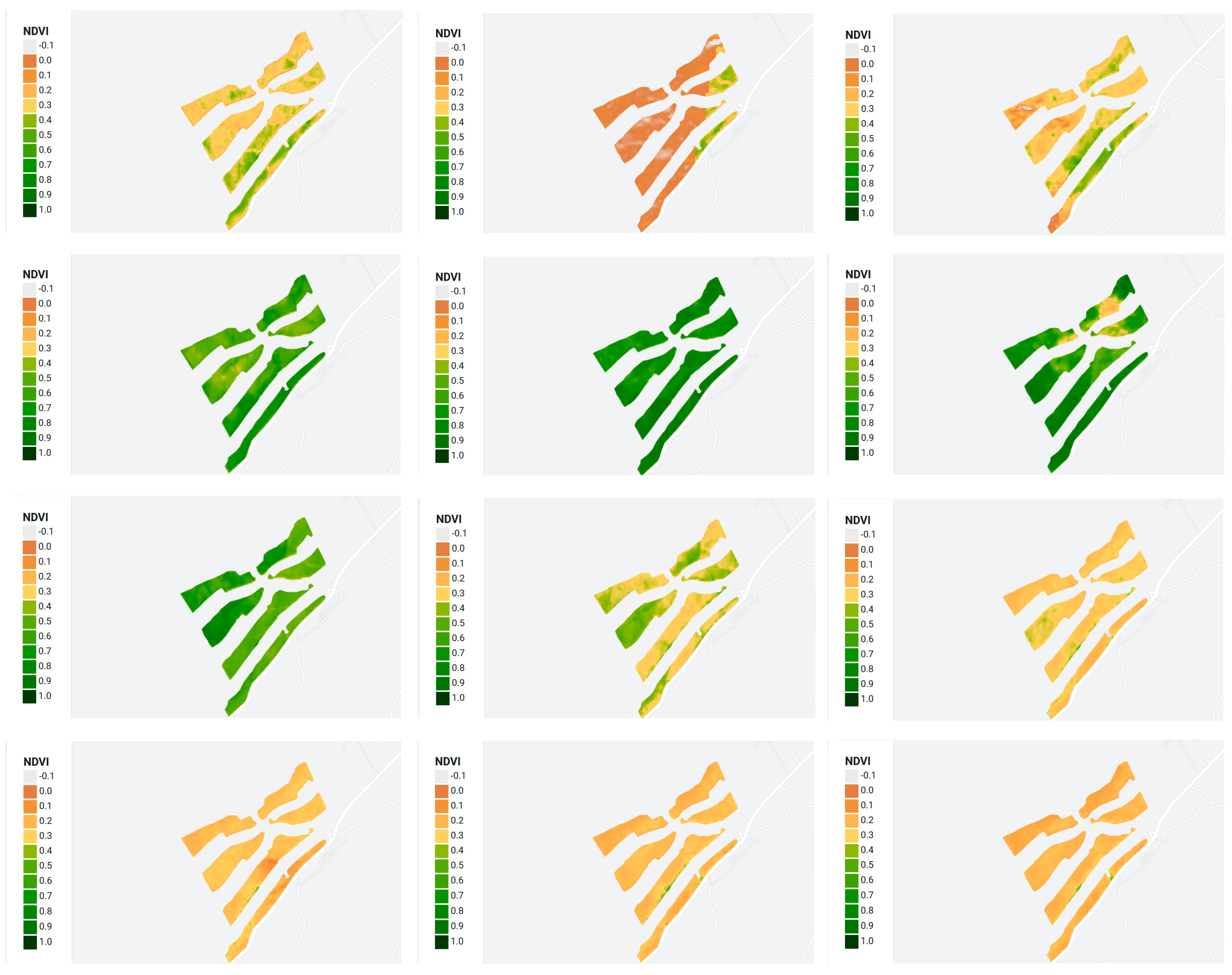
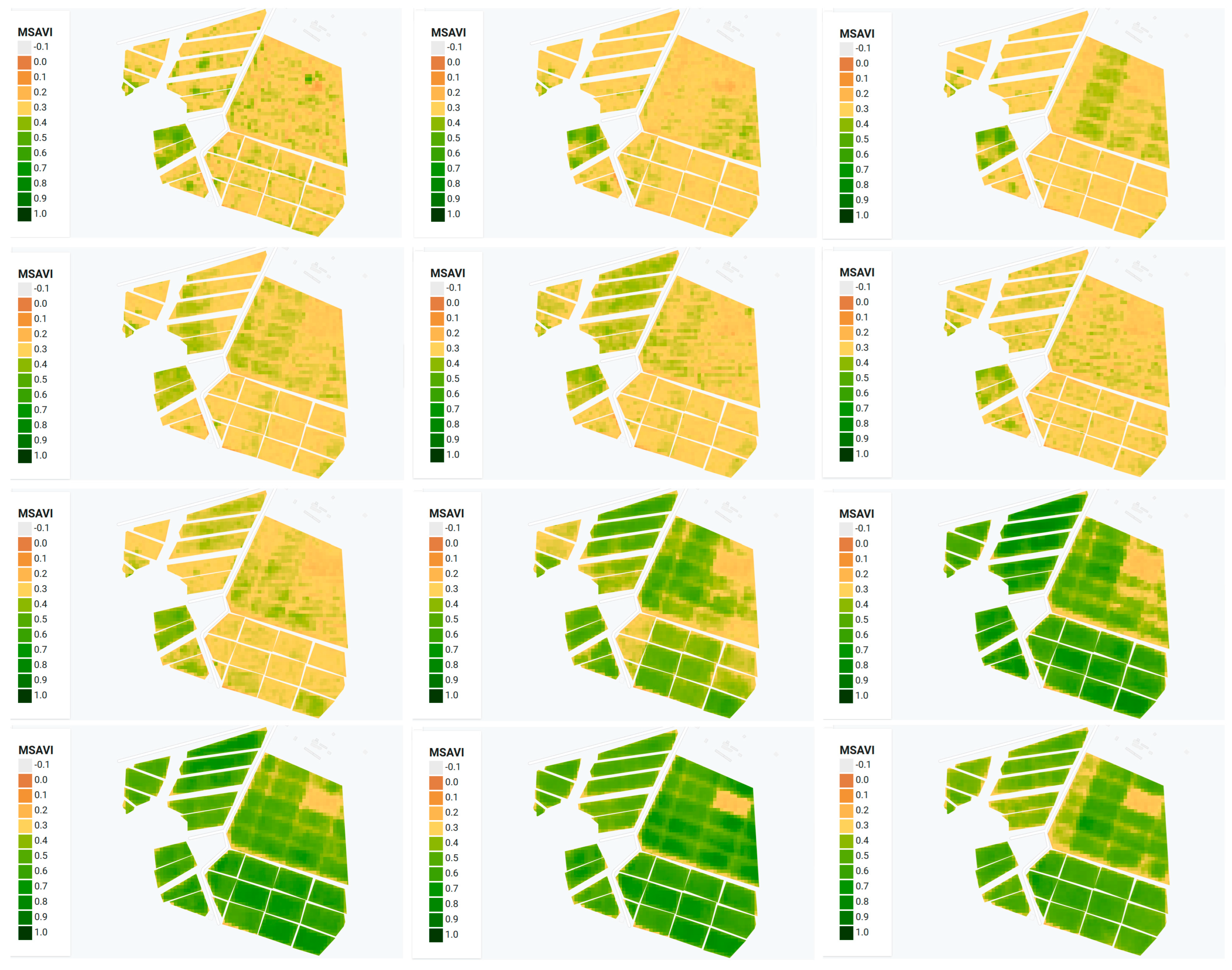
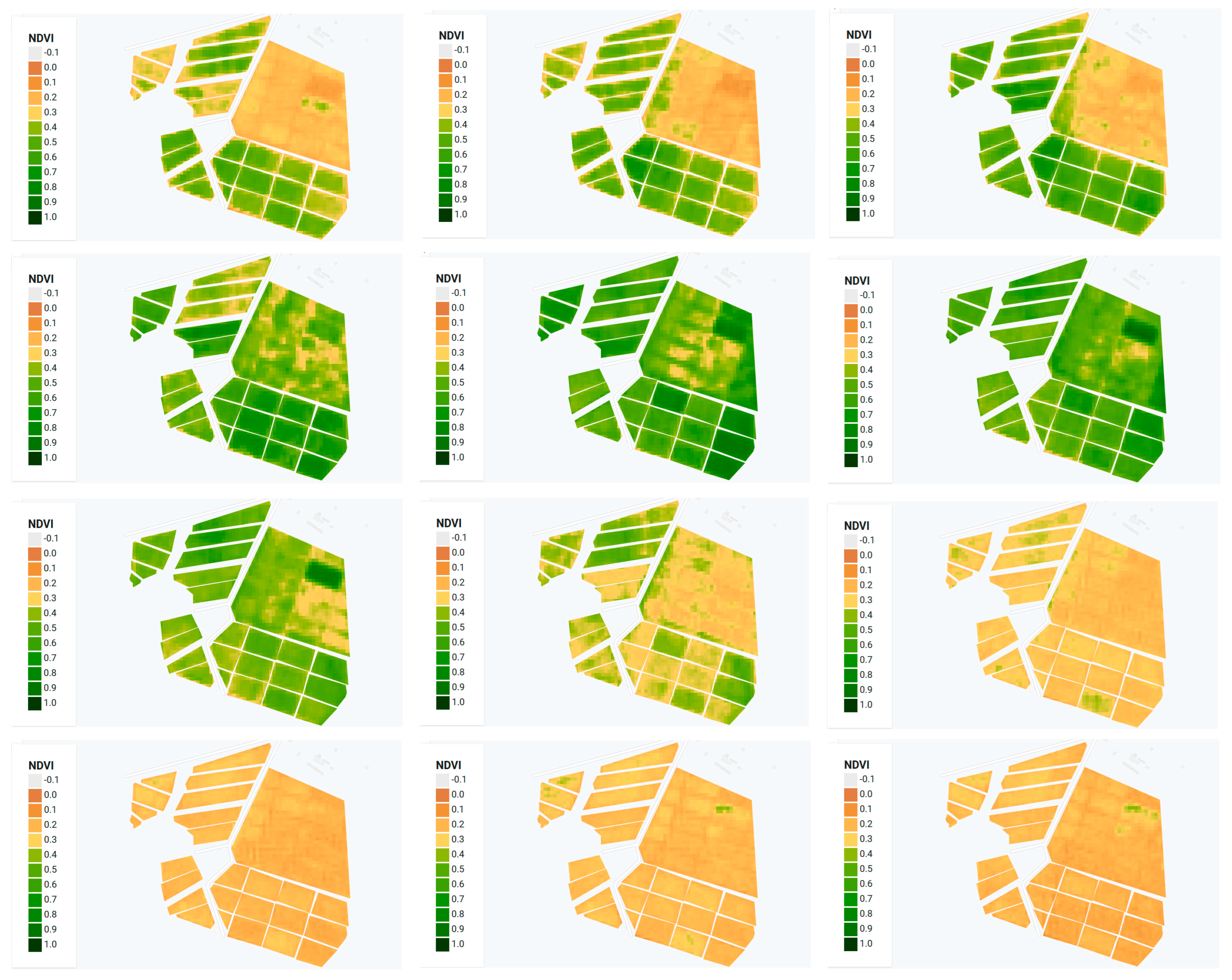
3.2. Phenological Development for the Two Vineyards through NDVI and MSAVI

Figure 6 shows the dynamics of NDVI and MSAVI of the mean of the plots for the two vineyards during the year 2022. As it is observed, the two spectral indices showed very similar dynamics in the two vineyards. NDVI and MSAVI began to increase on the 15th of April when the bud-break occurred. Then, during May and June, the two indices increased during leaf expansion. In VA, during May and June, values were higher than in PL due to the early development of some vine varieties (see Discussion). After that, spectral indices increased during leaf growth and flowering (except for a small decrease in VA at the end of June) until their maximum in mid-September, when most grapevine varieties were harvested.
Figure 7, Figure 8, Figure 9 and Figure 10 show the biweekly images of the NDVI and MSAVI for the two vineyards during the year 2022. From January to June, MSAVI was observed due to its ability to discriminate better in the first phenological stages than NDVI. Then, NDVI was shown from July to December.
These images are consistent with the dynamics of the mean plots shown in Figure 4 for both vineyards. In VA, the growing season started in mid-April in the southwest plots and the northwest plots. During May, all plots showed high MSAVI values, and during June, July, and August, MSAVI continued increasing. In September, NDVI values were their highest in most of the plots. From 2nd mid-October to November, NDVI decreased due to the fall of leaves. In PL, the dynamic was similar to that in VA. It must be highlighted that the growing season started a bit later than in VA and finished earlier in the southern plots than in the northern plots.

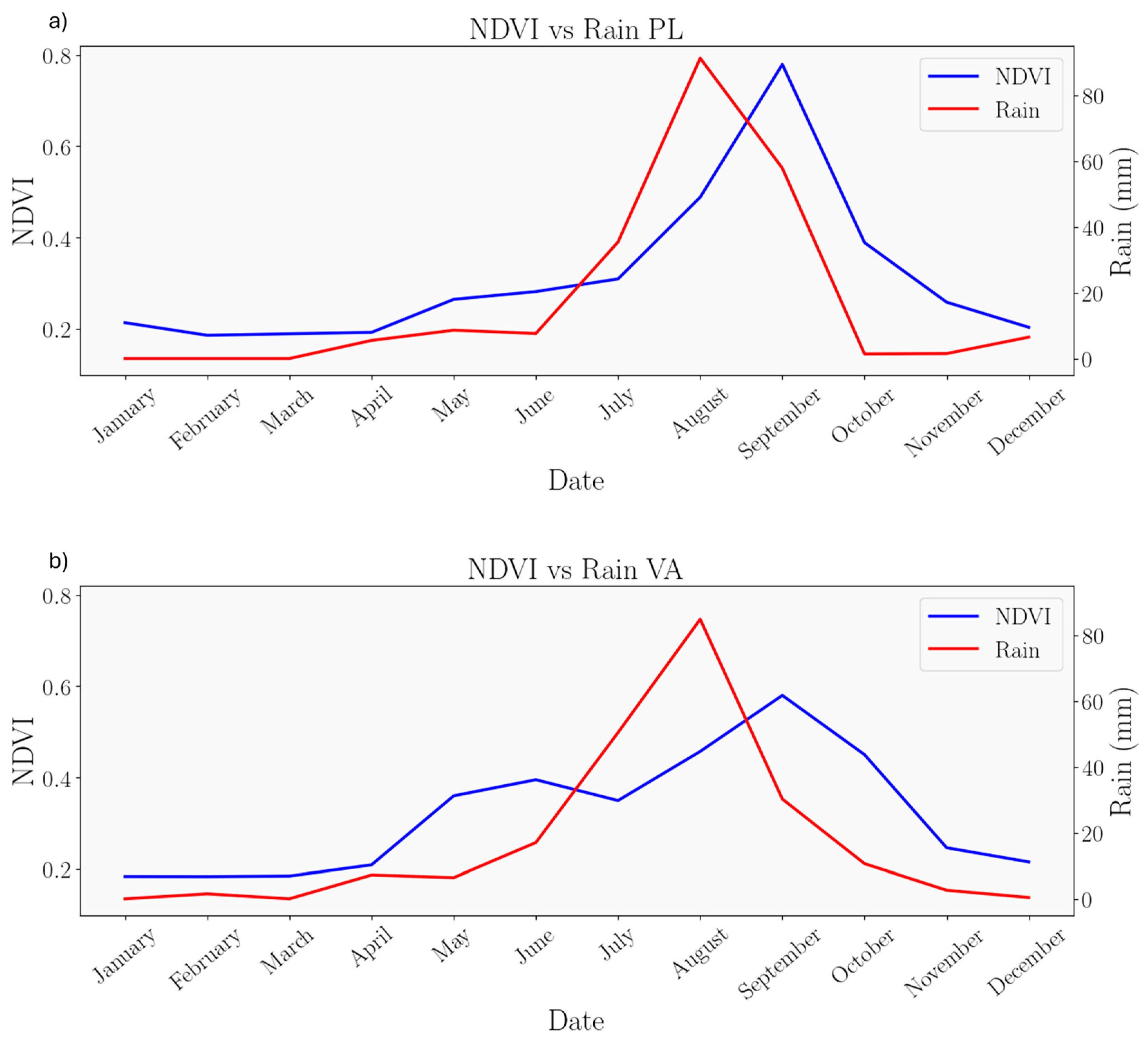
3.3. Relationship between NDVI and Precipitation

Figure 11 shows the dynamics of NDVI and precipitation obtained from CHIRPS in both sites. A high correlation was found between precipitation and NDVI, with a 15-day lag for PL and a one-month lag for VA. The correlation coefficients obtained were r = 0.82 for PL and r = 0.77   for VA, respectively. The complementary error function yielded values of 0.00057 for PL and 0.000174 for VA, indicating a substantial correlation between rainfall and NDVI. Hence, we assert with confidence the presence of a robust correlation between these variables.

3.4. Classification according to Thermal or Bioclimatic Indices

Table 5 shows the classification of the vineyards according to thermal indices obtained from the observations of the meteorological stations and the remote sensing data and reanalysis. As can be observed, the results obtained from both ways were perfectly compatible. In addition, Table 4 shows the classification of the vineyards through thermal indices for the period 2000–2022.
Although PL was classified as Winkler Region IV during 2022, the average for the period 2000–2022 showed that both vineyards were located in Winkler Zone III, similar to Rioja (Spain) or Sonoma Valley (California).
According to Huglin’s classification, the vineyards were located in a warm zone (2400–2700 °C), similar to Toro (Spain) or Napa Valley (California). This region is conducive to growing varieties well-suited to warmer climates, such as Cabernet Sauvignon, Grenache, Tempranillo, or Syrah.
Our vineyards are in the CI + 1 viticultural climate class according to Tonietto and Carbonneau [41], similar to Bordeaux (France), or Sonoma and Napa Valleys (California), where a maximum threshold of night temperature favourable to ripening will not be exceeded for any variety, as seen in Figure 5.
According to the GST index, the results obtained for 2022 from the data from the meteorological stations (19.4 °C for PL and 19.1 °C for VA) placed both vineyards at the lower limit of the warm zone. However, they were located in the temperate zone, taking into account the period 2000–2022. Therefore, they meet the phenological requirements for high- to premium-quality wine production with grapes cultivated in both vineyards.

4. Discussion

4.1. Spectral Indices and Phenology

The phenological development found based on spectral indices (NDVI and MSAVI) is consistent with the field information obtained about the different varieties. In this sense, Bramley et al. [57] used remote sensing data to identify zones of contrasting vineyard performance in a Cabernet Sauvignon vineyard in the Murray Valley region, obtaining satisfactory results. More recently, Vélez et al. [58] showed that NDVI provided by Sentinel-2 images could be used for an agronomic classification of three vineyards in Spain and an evaluation of their wines, and Pádua et al. [59] obtained a vineyard classification using multispectral data in three vineyards located in Portugal and Italy. In addition, Laroche-Pinel et al. [60] achieved an estimation of wine water status through Sentinel-2 spectral indices in France. Although there is little research in Central and South America with remote sensing applied to viticulture, the results were promising when it was used. Ramírez-Juidias et al. [61] used remote sensing images and they obtained yield estimations of the red globe grape variety in the North of Peru. In addition, García-Gutiérrez et al. [62] modelled the phenology in a cabernet sauvignon vineyard in Central Chile through data assimilation techniques and bioclimatic indices.
The main limitations of the study occurred during July and August (rainy season) due to clouds, which entailed low-quality images [63,64]. However, due to the high temporal resolution of Sentinel-2, the study of phenology could be assessed every 15 days.
In the present work, the phenology observed with the spectral indices was in accordance with the observed field data (personal communication and Table 2). Using the MSAVI index, we have observed that the first varieties to bud in VA are Chenin Blanc, Sauvignon Blanc, Syrah, and Chardonnay, towards the end of March, with the index response in the first half of April (see reference image). They are followed by Malbec, Marselan, Merlot, and Tempranillo, with the index response observed in the second half of April. The latest varieties, which bud in May, are Cabernet Franc, Riesling, and Gewürztraminer.
With the NDVI index, we observe significant differences within the same varieties. This is because some winegrowers are studying the effect of early defoliation (in June, Figure 6) on yield components, berry maturity, wine composition, and sensory properties of Malbec and Tempranillo vineyards (N-NE plots). The maximum NDVI value is found in September, when the harvest of all varieties ends, and from then on, the vines start to turn yellow, entering their period of seasonal rest.
Bud break in PL is slightly later, becoming noticeable in the second half of April, with the varieties Tempranillo, Macabeo, Xarel⋅Lo, Sauvignon Blanc, and Verdejo. Meanwhile, Syrah and Merlot vigorously bud in the first half of May. Due to high cloudiness between mid-July to mid-August, the NDVI index is not suitable. However, from the second half of August, we observe that the vineyard is at its peak (maximum greenness). From the first half of October, the vine leaves start to turn yellow, with Tempranillo being the last variety to lose its leaves.

4.2. Thermal Indices

On a worldwide scale, the typical range of temperatures that is considered suitable for viticulture, or grape cultivation, during the growing season falls between 12 °C and 22 °C in each hemisphere. This temperature range of 12–22 °C generally indicates that grape production is well-suited to mid-latitude regions. However, it’s worth noting that there are also many areas in higher elevations within sub-tropical to tropical zones that also fall within this climate range and are viable for winegrape cultivation [65].
In the present day, our understanding of the climate suitability for many well-known grape varieties worldwide reveals that the production of high-quality wine is most realistically achievable within the range of 13 °C to 21 °C for average growing season temperatures. Towards the upper end of this climatic spectrum, some grape production can still be successful, particularly in regions with average growing season temperatures exceeding 21 °C. However, such areas are primarily associated with the production of fortified wines, table grapes, and raisins (up to 24 °C) [66].
Winkler Region III and Huglin ‘Warm’ are both wine region classification systems that consider the climate and growing conditions of a particular area. In general, grapes that do well in warmer climates with longer growing seasons are better suited for Huglin ‘Warm’, while grapes that have a shorter ripening period and can tolerate cooler temperatures are more likely to thrive in Winkler Region III. Some grape varieties may be suitable for both Winkler Region III and Huglin ‘Warm’, such as Tempranillo, Chardonnay, Pinot Noir, Cabernet Franc, Sauvignon Blanc, Merlot, or Syrah.
GST ‘temperate’ indicates a region that has a moderate temperature during the growing season. In such a region, grapes that require a longer ripening period would be suitable. CI ‘cold’ indicates a region that experiences cold temperatures at night during the growing season. In such a region, grapes that are more resistant to cold and have a shorter ripening period would be suitable. Here are some grape varieties that may be suitable for GST ‘temperate’ and CI ‘cold’ regions: Pinot Noir, Chardonnay, Cabernet Franc, Gewürztraminer, Riesling, or Albariño. However, according to GST, a general warming trend was observed, and vineyards were shifting from the temperate zone to the warm zone. Some researchers are studying these changes in viticulture due to climate change [67,68]. Further research is needed to consider the effect of climate change and warming trends for future classifications of vineyards.

4.3. Meteorology, Dynamics, and Relations

In the two vineyards, the data obtained from the in-situ meteorological stations and the satellite data (temperature and precipitation) agreed perfectly, which assures us that we can use this methodology in other vineyards in the area that do not have a meteorological station. The climate in the area allows for the cultivation of various grape varieties. Temperature is not limiting for vine growth, although average minimum temperatures rounded 6 °C in December and January. However, these minimum temperatures did not occur in the growing period and frosts were not common in our study area. On the other hand, the lack of precipitation and soil moisture content are limiting factors for vine growth during the growing period, as corroborated by the high correlation found between precipitation and spectral indices with a one-month lag. Bonifacio et al. [69] also showed a similar period of response of vines to precipitation. The development of the vines in this region is linked to rainfall rather than irrigation or water stored in the subsurface, as observed in other regions [70]. However, a small amount of irrigation is necessary during the first stages of development of the vines during April and May (personal communication). Thus, droughts could be a special factor to consider for the development of vineyards in our study area, as other researchers have found in other regions [23,70].

5. Summary and Conclusions

The vineyards of Querétaro present a unique phenomenon in the viticultural world, as they deviate from the conventional “wine belt” typically found between latitudes 50° and 30° in both hemispheres. Situated as the southernmost wine region in the northern hemisphere, Querétaro boasts an altitude nearing 2000 m above sea level, enabling the cultivation of a diverse array of grape varieties and the production of wines of exceptional quality.
Results showed that spectral indices (MSAVI and NDVI) obtained from Sentinel-2 bands have adequately characterized the phenological dynamics of two vineyards in Queretaro (Mexico). While MSAVI was mainly useful for characterizing the first phenological stages of vineyards, NDVI was a good index to detect the last phenological stages of vineyards. Differences between varieties were detected using both indices.
In this region, precipitation and soil moisture content are limiting factors for vine growth during the growing period. In fact, due to the lack of precipitation during the first months of the year that could coincide with the bud-break of leaves, irrigation could be the only solution to avoid damage in the vineyards.
Thermal indices allow us to compare the vineyards with wine-growing areas throughout the world known for the excellent quality of their wines. These indices have shown that the best grape varieties are those that can adapt to both cooler and warmer temperatures, have a reasonable ripening period, and can produce wines with balanced acidity and flavours. Many of the varieties best adapted to the weather conditions are the ones cultivated in these vineyards. However, there are also successfully cultivated varieties that, at first glance, should not be as comfortable with these soil/rain/temperature combinations, such as Tempranillo, Malbec, or Sauvignon Blanc. This is due to the wide spectrum found, as some indices classify these vineyards as cool-temperate zones, while others classify them as temperate-warm zones. This successfully expands the range of possibilities when choosing a grape variety.
The combination of meteorological, remote sensing data, and thermal indices has managed to characterize the phenological dynamics of the different varieties of vineyards and to provide information for choosing the most suitable grape variety for this region.
This study has been conducted in vineyards equipped with meteorological stations, enabling the comparison of temperature and precipitation measurements with data obtained from various satellite sources. The high degree of agreement between these datasets makes us confident to extend this study to other smaller vineyards that do not have adequate equipment or available land for new vineyard development. This type of study does not require investment on the part of the winegrowers, and once the process is learned, the technicians can monitor the dynamics of the vineyard. Thus, it is a first step to use remote sensing data in combination with thermal indices to characterize vineyards in developing countries. Further research is needed to apply this study to other vineyards and a longer period.

Author Contributions

Conceptualisation, M.S.d.R., V.C. and C.Y.; methodology, M.S.d.R. and V.C.; investigation, M.S.d.R., V.C. and C.Y.; data curation, M.S.d.R. and V.C.; writing—original draft preparation, M.S.d.R. and V.C.; writing—review and editing, M.S.d.R., V.C. and C.Y. All authors have read and agreed to the published version of the manuscript.

Funding

Víctor Cicuéndez was supported by a post-doctoral Juan de la Cierva fellowship (FJC2021-046735-I) funded by the Spanish Ministerio de Ciencia e Innovación MCIN/AEI/10.13039/501100011033 and by the European Union’s «NextGenerationEU»/PRTR». María Soledad del Rio was supported by the Funding for Academic, Scientific, Technological Development and Creative Projects Program from Arkansas State University, Campus Querétaro.

Data Availability Statement

The authors confirm that the data supporting the findings of this study are available within the article.

Acknowledgments

The authors want to thank E. Goyeneche and C. Armas, from Puerta del Lobo, and H.L. Duer and L. Gallardo, from Vinaltura, for their generous help when collecting data from their respective vineyards.

Conflicts of Interest

The authors declare no conflicts of interest. The funders had no role in the design of the study; in the collection, analyses, or interpretation of data; in the writing of the manuscript; or in the decision to publish the results.

References

  1. OIV International Organisation of Vine and Wine. Available online: https://www.oiv.int/ (accessed on 16 October 2023).
  2. Yu, Y.; Rodrigo-Comino, J. Analyzing Regional Geographic Challenges: The Resilience of Chinese Vineyards to Land Degradation Using a Societal and Biophysical Approach. Land 2021, 10, 227. [Google Scholar] [CrossRef]
  3. Uvayvino.Org. Available online: https://uvayvino.org.mx/ (accessed on 16 October 2023).
  4. Cruz-de Aquino, M.A.d.l.; Martínez-Peniche, R.A.; Becerril-Román, A.E.; Chávaro-Ortiz, M.d.S. Physical and Chemical Characterization of Red Wines Produced in Querétaro. Rev. Fitotec. Mex. 2012, 35, 61–67. [Google Scholar]
  5. Sun, Q.; Granco, G.; Groves, L.; Voong, J.; Van Zyl, S. Viticultural Manipulation and New Technologies to Address Environmental Challenges Caused by Climate Change. Climate 2023, 11, 83. [Google Scholar] [CrossRef]
  6. Weiss, M.; Jacob, F.; Duveiller, G. Remote Sensing for Agricultural Applications: A Meta-Review. Remote Sens. Environ. 2020, 236, 111402. [Google Scholar] [CrossRef]
  7. Palacios-Orueta, A.; Huesca, M.; Whiting, M.L.; Litago, J.; Khanna, S.; Garcia, M.; Ustin, S.L. Derivation of Phenological Metrics by Function Fitting to Time-Series of Spectral Shape Indexes AS1 and AS2: Mapping Cotton Phenological Stages Using MODIS Time Series. Remote Sens. Environ. 2012, 126, 148–159. [Google Scholar] [CrossRef]
  8. Cicuéndez, V.; Rodríguez-Rastrero, M.; Huesca, M.; Uribe, C.; Schmid, T.; Inclán, R.; Litago, J.; Sánchez-Girón, V.; Merino-de-Miguel, S.; Palacios-Orueta, A. Assessment of Soil Respiration Patterns in an Irrigated Corn Field Based on Spectral Information Acquired by Field Spectroscopy. Agric. Ecosyst. Environ. 2015, 212, 158–167. [Google Scholar] [CrossRef]
  9. Viña, A.; Gitelson, A.A.; Nguy-Robertson, A.L.; Peng, Y. Comparison of Different Vegetation Indices for the Remote Assessment of Green Leaf Area Index of Crops. Remote Sens. Environ. 2011, 115, 3468–3478. [Google Scholar] [CrossRef]
  10. Tucker, C.J. Red and Photographic Infrared Linear Combinations for Monitoring Vegetation. Remote Sens. Environ. 1979, 8, 127–150. [Google Scholar] [CrossRef]
  11. Huete, A.; Didan, K.; Miura, T.; Rodriguez, E.P.; Gao, X.; Ferreira, L.G. Overview of the Radiometric and Biophysical Performance of the MODIS Vegetation Indices. Remote Sens. Environ. 2002, 83, 195–213. [Google Scholar] [CrossRef]
  12. Qi, J.; Chehbouni, A.; Huete, A.R.; Kerr, Y.H.; Sorooshian, S. A Modified Soil Adjusted Vegetation Index. Remote Sens. Environ. 1994, 48, 119–126. [Google Scholar] [CrossRef]
  13. Huete, A.R. A Soil-Adjusted Vegetation Index (SAVI). Remote Sens. Environ. 1988, 25, 295–309. [Google Scholar] [CrossRef]
  14. Hall, A.; Lamb, D.W.; Holzapfel, B.; Louis, J. Optical Remote Sensing Applications in Viticulture—A Review. Aust. J. Grape Wine Res. 2002, 8, 36–47. [Google Scholar] [CrossRef]
  15. Kazmierski, M.; Glémas, P.; Rousseau, J.; Tisseyre, B. Temporal Stability of Within-Field Patterns of NDVI in Non Irrigated Mediterranean Vineyards. OENO One 2011, 45, 61. [Google Scholar] [CrossRef]
  16. Puig-Sirera, À.; Antichi, D.; Warren Raffa, D.; Rallo, G. Application of Remote Sensing Techniques to Discriminate the Effect of Different Soil Management Treatments over Rainfed Vineyards in Chianti Terroir. Remote Sens. 2021, 13, 716. [Google Scholar] [CrossRef]
  17. Badr, G.; Hoogenboom, G.; Davenport, J.; Smithyman, J. Estimating Growing Season Length Using Vegetation Indices Based on Remote Sensing: A Case Study for Vineyards in Washington State. Trans. ASABE 2015, 58, 551–564. [Google Scholar] [CrossRef]
  18. Zorer, R.; Rocchini, D.; Metz, M.; Delucchi, L.; Zottele, F.; Meggio, F.; Neteler, M. Daily MODIS Land Surface Temperature Data for the Analysis of the Heat Requirements of Grapevine Varieties. IEEE Trans. Geosci. Remote Sens. 2013, 51, 2128–2135. [Google Scholar] [CrossRef]
  19. Shammi, S.A.; Meng, Q. Use Time Series NDVI and EVI to Develop Dynamic Crop Growth Metrics for Yield Modeling. Ecol. Indic. 2021, 121, 107124. [Google Scholar] [CrossRef]
  20. Ribeiro, L.F.O.; da Vitória, E.L.; Soprani Júnior, G.G.; Chen, P.; Lan, Y. Impact of Operational Parameters on Droplet Distribution Using an Unmanned Aerial Vehicle in a Papaya Orchard. Agronomy 2023, 13, 1138. [Google Scholar] [CrossRef]
  21. Gavrilović, M.; Jovanović, D.; Božović, P.; Benka, P.; Govedarica, M. Vineyard Zoning and Vine Detection Using Machine Learning in Unmanned Aerial Vehicle Imagery. Remote Sens. 2024, 16, 584. [Google Scholar] [CrossRef]
  22. Atencia Payares, L.K.; Tarquis, A.M.; Hermoso Peralo, R.; Cano, J.; Cámara, J.; Nowack, J.; Gómez del Campo, M. Multispectral and Thermal Sensors Onboard UAVs for Heterogeneity in Merlot Vineyard Detection: Contribution to Zoning Maps. Remote Sens. 2023, 15, 4024. [Google Scholar] [CrossRef]
  23. Cogato, A.; Pagay, V.; Marinello, F.; Meggio, F.; Grace, P.; Migliorati, M.D.A. Assessing the Feasibility of Using Sentinel-2 Imagery to Quantify the Impact of Heatwaves on Irrigated Vineyards. Remote Sens. 2019, 11, 2869. [Google Scholar] [CrossRef]
  24. Cogato, A.; Meggio, F.; Collins, C.; Marinello, F. Medium-Resolution Multispectral Data from Sentinel-2 to Assess the Damage and the Recovery Time of Late Frost on Vineyards. Remote Sens. 2020, 12, 1896. [Google Scholar] [CrossRef]
  25. García-gutiérrez, V.; Stöckle, C.; Gil, P.M.; Meza, F.J. Evaluation of Penman–Monteith Model Based on Sentinel-2 Data for the Estimation of Actual Evapotranspiration in Vineyards. Remote Sens. 2021, 13, 478. [Google Scholar] [CrossRef]
  26. Devaux, N.; Crestey, T.; Leroux, C.; Tisseyre, B. Potential of Sentinel-2 Satellite Images to Monitor Vine Fields Grown at a Territorial Scale. OENO One 2019, 53, 51–58. [Google Scholar] [CrossRef]
  27. Stolarski, O.; Fraga, H.; Sousa, J.J.; Pádua, L. Synergistic Use of Sentinel-2 and UAV Multispectral Data to Improve and Optimize Viticulture Management. Drones 2022, 6, 366. [Google Scholar] [CrossRef]
  28. Vélez, S.; Rançon, F.; Barajas, E.; Brunel, G.; Rubio, J.A.; Tisseyre, B. Potential of Functional Analysis Applied to Sentinel-2 Time-Series to Assess Relevant Agronomic Parameters at the within-Field Level in Viticulture. Comput. Electron. Agric. 2022, 194, 106726. [Google Scholar] [CrossRef]
  29. Giovos, R.; Tassopoulos, D.; Kalivas, D.; Lougkos, N.; Priovolou, A. Remote Sensing Vegetation Indices in Viticulture: A Critical Review. Agriculture 2021, 11, 457. [Google Scholar] [CrossRef]
  30. Fernandez-Beltran, R.; Baidar, T.; Kang, J.; Pla, F. Rice-Yield Prediction with Multi-Temporal Sentinel-2 Data and 3D CNN: A Case Study in Nepal. Remote Sens. 2021, 13, 1391. [Google Scholar] [CrossRef]
  31. Phiri, D.; Simwanda, M.; Salekin, S.; Nyirenda, V.; Murayama, Y.; Ranagalage, M. Sentinel-2 Data for Land Cover/Use Mapping: A Review. Remote Sens. 2020, 12, 2291. [Google Scholar] [CrossRef]
  32. Sustainable Development Goals. Available online: https://sdgs.un.org/goals (accessed on 16 October 2023).
  33. Jones, G.V. Climate Change in the Western United States Grape Growing Regions. Acta Hortic. 2005, 689, 41–60. [Google Scholar] [CrossRef]
  34. Karoglan, M.; Telišman Prtenjak, M.; Šimon, S.; Osrečak, M.; Anić, M.; Karoglan Kontić, J.; Andabaka, Ž.; Tomaz, I.; Grisogono, B.; Belušić, A.; et al. Classification of Croatian Winegrowing Regions Based on Bioclimatic Indices. In Proceedings of the XII International Terroir Congress, Zaragoza, Spain, 22 June 2018; p. 01032. [Google Scholar]
  35. Badr, G.; Hoogenboom, G.; Abouali, M.; Moyer, M.; Keller, M. Analysis of Several Bioclimatic Indices for Viticultural Zoning in the Pacific Northwest. Clim. Res. 2018, 76, 203–223. [Google Scholar] [CrossRef]
  36. Amerine, M.; Winkler, A. Composition and Quality of Musts and Wines of California Grapes. Hilgardia 1944, 15, 493–675. [Google Scholar] [CrossRef]
  37. Winkler, A.J. General Viticulture; University of California Press: Berkeley, CA, USA, 1974. [Google Scholar]
  38. Huglin, P. Nouveau Mode d’évaluation Des Possibilités Héliothermiques d’un Milieu Viticole. Comptes Rendus de l’Académie d’Agriculture; Académie d’agriculture de France: Paris, France, 1978.
  39. Jones, G.V. Climate and Terroir: Impacts of Climate Variability and Change on Wine. In Fine Wine and Terroir—The Geoscience Perspective; Macqueen, R.W., Meinert, L.D., Eds.; Geological Association of Canada: St John’s, NL, Canada, 2006; pp. 203–216. [Google Scholar]
  40. Tonietto, J. Les Macroclimats Viticoles Mondiaux et l’influence Du Mésoclimat Sur La Typicité de La Syrah et Du Muscat de Hambourg 447 Dans Le Sud de La France: Méthodologie de Caráctérisation; Ecole Nationale Supérieure Agronomique: Montpellier, France, 1999. [Google Scholar]
  41. Tonietto, J.; Carbonneau, A. A Multicriteria Climatic Classification System for Grape-Growing Regions Worldwide. Agric. Meteorol. 2004, 124, 81–97. [Google Scholar] [CrossRef]
  42. Honorio, F.; García-Martín, A.; Moral, F.J.; Paniagua, L.L.; Rebollo, F.J. Spanish Vineyard Classification According to Bioclimatic Indexes. Aust. J. Grape Wine Res. 2018, 24, 335–344. [Google Scholar] [CrossRef]
  43. del Río, M.S.; Raventós, L.; Garza, V. Zoning of the Querétaro Wine Region. BIO Web Conf. 2023, 68, 01029. [Google Scholar] [CrossRef]
  44. Beck, H.E.; Zimmermann, N.E.; McVicar, T.R.; Vergopolan, N.; Berg, A.; Wood, E.F. Present and Future Köppen-Geiger Climate Classification Maps at 1-Km Resolution. Sci. Data 2018, 5, 180214. [Google Scholar] [CrossRef] [PubMed]
  45. European Space Agency. Available online: www.esa.int (accessed on 16 October 2023).
  46. Farr, T.G.; Rosen, P.A.; Caro, E.; Crippen, R.; Duren, R.; Hensley, S.; Kobrick, M.; Paller, M.; Rodriguez, E.; Roth, L.; et al. The Shuttle Radar Topography Mission. Rev. Geophys. 2007, 45, RG2004. [Google Scholar] [CrossRef]
  47. Muñoz-Sabater, J.; Dutra, E.; Agustí-Panareda, A.; Albergel, C.; Arduini, G.; Balsamo, G.; Boussetta, S.; Choulga, M.; Harrigan, S.; Hersbach, H.; et al. ERA5-Land: A State-of-the-Art Global Reanalysis Dataset for Land Applications. Earth Syst. Sci. Data 2021, 13, 4349–4383. [Google Scholar] [CrossRef]
  48. Thornton, M.M.; Shrestha, R.; Wei, Y.; Thornton, P.E.; Kao, S.; Wilson, B.E. Daymet: Daily Surface Weather Data on a 1-Km Grid for North America, Version 4; ORNL DAAC: Oak Ridge, TN, USA, 2020.
  49. Funk, C.; Peterson, P.; Landsfeld, M.; Pedreros, D.; Verdin, J.; Shukla, S.; Husak, G.; Rowland, J.; Harrison, L.; Hoell, A.; et al. The Climate Hazards Infrared Precipitation with Stations—A New Environmental Record for Monitoring Extremes. Sci. Data 2015, 2, 150066. [Google Scholar] [CrossRef]
  50. Eos Data Analytics. Available online: https://www.eos.com/ (accessed on 13 September 2023).
  51. Goldammer, T. The Grape Grower’s Handbook: A Guide to Viticulture for Wine Production; Apex Publishers: Centreville, VA, USA, 2018. [Google Scholar]
  52. Meyers, J.M.; Vanden Heuvel, J.E. Use of Normalized Difference Vegetation Index Images to Optimize Vineyard Sampling Protocols. Am. J. Enol. Vitic. 2014, 65, 250–253. [Google Scholar] [CrossRef]
  53. Martínez, A.; Gomez-Miguel, V.D. Vegetation Index Cartography as a Methodology Complement to the Terroir Zoning for Its Use in Precision Viticulture. OENO One 2017, 51, 289. [Google Scholar] [CrossRef]
  54. Ferro, M.V.; Catania, P.; Miccichè, D.; Pisciotta, A.; Vallone, M.; Orlando, S. Assessment of Vineyard Vigour and Yield Spatio-Temporal Variability Based on UAV High Resolution Multispectral Images. Biosyst. Eng. 2023, 231, 36–56. [Google Scholar] [CrossRef]
  55. Blanco-Ward, D.; Ribeiro, A.; Barreales, D.; Castro, J.; Verdial, J.; Feliciano, M.; Viceto, C.; Rocha, A.; Carlos, C.; Silveira, C.; et al. Climate Change Potential Effects on Grapevine Bioclimatic Indices: A Case Study for the Portuguese Demarcated Douro Region (Portugal). BIO Web Conf. 2019, 12, 01013. [Google Scholar] [CrossRef]
  56. Press, W.H. Numerical Recipes 3rd Edition: The Art of Scientific Computing; Cambridge University Press, Ed.; Cambridge University Press: Cambridge, UK, 2007. [Google Scholar]
  57. Bramley, R.G.V.; Ouzman, J.; Boss, P.K. Variation in Vine Vigour, Grape Yield and Vineyard Soils and Topography as Indicators of Variation in the Chemical Composition of Grapes, Wine and Wine Sensory Attributes. Aust. J. Grape Wine Res. 2011, 17, 217–229. [Google Scholar] [CrossRef]
  58. Vélez, S.; Rubio, J.A.; Andrés, M.I.; Barajas, E. Agronomic Classification between Vineyards (‘Verdejo’) Using NDVI and Sentinel-2 and Evaluation of Their Wines. Vitis J. Grapevine Res. 2019, 58, 33–38. [Google Scholar] [CrossRef]
  59. Pádua, L.; Matese, A.; Di Gennaro, S.F.; Morais, R.; Peres, E.; Sousa, J.J. Vineyard Classification Using OBIA on UAV-Based RGB and Multispectral Data: A Case Study in Different Wine Regions. Comput. Electron. Agric. 2022, 196, 106905. [Google Scholar] [CrossRef]
  60. Laroche-Pinel, E.; Duthoit, S.; Albughdadi, M.; Costard, A.D.; Rousseau, J.; Chéret, V.; Clenet, H. Towards Vine Water Status Monitoring on a Large Scale Using Sentinel-2 Images. Remote Sens. 2021, 13, 1837. [Google Scholar] [CrossRef]
  61. Ramírez-Juidias, E.; Amaro-Mellado, J.-L.; Leiva-Piedra, J.L.; Mediano-Guisado, J.A. Use of Remote Sensing Techniques to Infer the Red Globe Grape Variety in the Chancay-Lambayeque Valley (Northern Peru). Remote Sens. Appl. 2024, 33, 101108. [Google Scholar] [CrossRef]
  62. García-Gutiérrez, V.; Meza, F. Modeling Phenology Combining Data Assimilation Techniques and Bioclimatic Indices in a Cabernet Sauvignon Vineyard (Vitis vinifera L.) in Central Chile. Remote Sens. 2023, 15, 3537. [Google Scholar] [CrossRef]
  63. Coluzzi, R.; Imbrenda, V.; Lanfredi, M.; Simoniello, T. A First Assessment of the Sentinel-2 Level 1-C Cloud Mask Product to Support Informed Surface Analyses. Remote Sens. Environ. 2018, 217, 426–443. [Google Scholar] [CrossRef]
  64. Nazarova, T.; Martin, P.; Giuliani, G. Monitoring Vegetation Change in the Presence of High Cloud Cover with Sentinel-2 in a Lowland Tropical Forest Region in Brazil. Remote Sens. 2020, 12, 1829. [Google Scholar] [CrossRef]
  65. Jones, G.V.; Reid, R.; Vilks, A. Climate, Grapes, and Wine: Structure and Suitability in a Variable and Changing Climate. In The Geography of Wine; Dougherty, P., Ed.; Springer: Dordrecht, The Netherlands, 2012; pp. 109–133. [Google Scholar]
  66. Jones, G.V.; Alves, F. Impact of Climate Change on Wine Production: A Global Overview and Regional Assessment in the Douro Valley of Portugal. Int. J. Glob. Warm. 2012, 4, 383. [Google Scholar] [CrossRef]
  67. Omazić, B.; Telišman Prtenjak, M.; Bubola, M.; Meštrić, J.; Karoglan, M.; Prša, I. Application of Statistical Models in the Detection of Grapevine Phenology Changes. Agric. Meteorol. 2023, 341, 109682. [Google Scholar] [CrossRef]
  68. Droulia, F.; Charalampopoulos, I. A Review on the Observed Climate Change in Europe and Its Impacts on Viticulture. Atmosphere 2022, 13, 837. [Google Scholar] [CrossRef]
  69. Bonifacio, R.; Dugdale, G.; Milford, J.R. Sahelian Rangeland Production in Relation to Rainfall Estimates from Meteosat. Int. J. Remote Sens. 1993, 14, 2695–2711. [Google Scholar] [CrossRef]
  70. De la Casa, A.; Ovando, G. Relación Entre La Precipitación e Índices de Vegetación Durante El Comienzo Del Ciclo Anual de Lluvias En La Provincia de Córdoba, Argentina. RIA Rev. Investig. Agropecu. 2006, 35, 67–85. [Google Scholar]
Figure 1. Queretaro in the world. Images were taken from the ESRI satellite for QGIS.
Remotesensing 16 02538 g001
Figure 2. Images from Google Satellite of the studied vineyards: (a) Puerta del Lobo (PL) and (b) Vinaltura (VA).
Remotesensing 16 02538 g002
Figure 3. Monthly rainfall and average maximum (red line) and minimum (blue line) monthly temperatures for the period 1981-2023: (a) Puerta del Lobo and (b) Vinaltura. The black triangles and the orange circles correspond to the values for the year 2022.
Remotesensing 16 02538 g003aRemotesensing 16 02538 g003b
Figure 4. Dynamics of the studied meteorological variables in the two vineyards during year 2022: (a) dynamics of temperature (°C) and precipitation (mm) in Puerta del Lobo (PL), (b) dynamics of temperature (°C) and precipitation (mm) in VA, (c) dynamics of relative humidity (%) and dew Point (°C) in PL, and (d) dynamics of relative humidity (%) and dew point (°C) in Vinaltura (VA).
Remotesensing 16 02538 g004aRemotesensing 16 02538 g004b
Figure 5. Maximal and minimal daily temperatures in Puerta del Lobo (PL) (a) and in Vinaltura (VA) (b) for the year 2022.
Remotesensing 16 02538 g005
Figure 6. Dynamics of the spectral vegetation indices, NDVI and MSAVI, of the mean of the plots for the two vineyards: (a) Puerta del Lobo (PL) and (b) Vinaltura (VA) for the year 2022. The letters are the different phenological stages identified in field, shown in Table 2: S—Sprouting, LA—Leaf Appearance, F—Flowering, V—Veraison, H—Harvest, B—Browning of leaves.
Remotesensing 16 02538 g006
Figure 7. MSAVI maps showing every 15 days from January to June 2022 for Puerta del Lobo (PL).
Remotesensing 16 02538 g007
Figure 8. NDVI maps showing every 15 days from July to December 2022 for Puerta del Lobo (PL).
Remotesensing 16 02538 g008
Figure 9. MSAVI maps showing every 15 days from January to June 2022 for Vinaltura (VA).
Remotesensing 16 02538 g009
Figure 10. NDVI maps showing every 15 days from July to December 2022 for Vinaltura (VA).
Remotesensing 16 02538 g010
Figure 11. Dynamics of NDVI and precipitation obtained from CHIRPS in Puerta del Lobo (PL) (a) and Vinaltura (VA) (b) for the year 2022.
Remotesensing 16 02538 g011
Table 1. Characteristics of both vineyards: Puerta del Lobo (PL) and Vinaltura (VA). Annual precipitation and average temperature for the period 1981–2023.
VineyardArea (Ha)Average Temperature (°C)Annual Precipitation (mm)Primary SoilSecondary SoilAltitude (masl)Mean Slope
PL22.717.6521.4Vertisol/LeptosolPhaeozems19503.8°
VA23.817.5472.5VertisolVertisol19672.4°
Table 2. The average date for all the varieties of the main phenological stages recollected in the field by the winegrowers in the two vineyards.
PLVA
Pruning 13 March 2022
Sprouting20 March 202221 March 2022
First leaves appearance7 April 20221 April 2022
Flowering2 May 20223 May 2022
Veraison (50%)10 July 20228 July 2022
Harvest19 August 202217 August 2022
Browning of leaves17 October 202218 October 2022
Table 3. Range values for NDVI and interpretation.
ValueInterpretation
<0.1Bare soil, water, or clouds
0.1–0.2Almost absent canopy cover
0.2–0.3Very low canopy cover
0.3–0.4Low canopy cover with low vigour or very low canopy cover with high vigour
0.4–0.5Mid-low canopy cover with low vigour or low canopy cover with high vigour
0.5–0.6Average canopy cover with low vigour or mid-low canopy cover with high vigour
0.6–0.7Mid-high canopy cover with low vigour or average canopy cover with high vigour
0.7–0.8High canopy cover with high vigour
0.8–0.9Very high canopy cover with very high vigour
0.9–1.0Total canopy cover with very high vigour
Table 4. Range values for MSAVI and their interpretation.
ValueInterpretation
−1.0–0.2Bare soil
0.2–0.4Seed germination stage
0.4–0.6Leaf development stage
>0.6Vegetation is dense enough to cover the soil, use NDVI
Table 5. Classification of the vineyards according to thermal indices obtained from the observations of the meteorological stations and the remote sensing data for 2022, and the classification of the vineyards through thermal indices for the period 2000–2022.
IndexPLVA
Local Meteorological StationsWI2020 °C Region IV1911 °C Region III
HI2541 °C Warm2442 °C Warm
GST19.4° C Warm19.1 °C Warm
CI12.4 °C Cold12.3 °C Cold
SatellitesWI2019 °C Region IV1934 °C Region III
HI2652 °C Warm2654 °C Warm
GST19.4 °C Warm19.0 °C Warm
CI13.1 °C Cold13.2 °C Cold
Average
2000–2022
WIRegion IIIRegion III
HIWarmWarm
GSTTemperateTemperate
CIColdCold
Disclaimer/Publisher’s Note: The statements, opinions and data contained in all publications are solely those of the individual author(s) and contributor(s) and not of MDPI and/or the editor(s). MDPI and/or the editor(s) disclaim responsibility for any injury to people or property resulting from any ideas, methods, instructions or products referred to in the content.

