Abstract
Total nitrogen (TN) is a critical nutrient for plant growth, and its monitoring in agricultural soil is vital for farm managers. Traditional methods of estimating soil TN levels involve laborious and costly chemical analyses, especially when applied to large areas with multiple sampling points. Remote sensing offers a promising alternative for identifying, tracking, and mapping soil TN levels at various scales, including the field, landscape, and regional levels. Spaceborne hyperspectral sensing has shown effectiveness in reflecting soil TN levels. This study evaluates the efficiency of spectral reflectance at visible near-infrared (VNIR) and shortwave near-infrared (SWIR) regions to identify the most informative hyperspectral bands responding to the TN content in agricultural soil. In this context, we used PRISMA (PRecursore IperSpettrale della Missione Applicativa) hyperspectral imagery with ensemble learning modeling to identify N-specific absorption features. This ensemble consisted of three multivariate regression techniques, partial least square (PLSR), support vector regression (SVR), and Gaussian process regression (GPR) learners. The soil TN data (n = 803) were analyzed against a hyperspectral PRISMA imagery to perform spectral band selection. The 803 sampled data points were derived from open-access soil property and nutrient maps for Africa at a 30 m resolution over a bare agricultural field in southern Morocco. The ensemble learning strategy identified several bands in the SWIR in the regions of 900–1300 nm and 1900–2200 nm. The models achieved coefficient-of-determination values ranging from 0.63 to 0.73 and root-mean-square error values of 0.14 g/kg for PLSR, 0.11 g/kg for SVR, and 0.12 g/kg for GPR, which had been boosted to an R2 of 0.84, an RMSE of 0.08 g/kg, and an RPD of 2.53 by the ensemble, demonstrating the model’s accuracy in predicting the soil TN content. These results underscore the potential for using spaceborne hyperspectral imagery for soil TN estimation, enabling the development of decision-support tools for variable-rate fertilization and advancing our understanding of soil spectral responses for improved soil management.
1. Introduction
Nitrogen (N) is among the most important agricultural inputs [1] to enhance crop growth. Typically, crop growth responds to the addition of fertilizers, emphasizing their significance in terms of agricultural yield performance [2]. Typically, established techniques including routine soil sampling and subsequent soil chemical analyses are used to evaluate TN levels. Point-scale (i.e., discrete) data on TN levels in soil are obtained using conventional soil-testing techniques [3]. Nonetheless, it is generally acknowledged that these procedures are costly and labor consuming, particularly for monitoring soil TN throughout large croplands on an annual basis. As a result, developing and implementing an in situ, low-cost, and quick analytical method is critical for regular soil fertility assessments.
Soil reflectance spectroscopy over the whole spectrum (i.e., visible near-infrared (VNIR) and shortwave infrared (SWIR) regions) is an approach that has proven to be a quick, inexpensive, and nondestructive alternative method of soil elemental analyses [4,5] including N. This approach has been utilized routinely in the laboratory with proven applications in situ as well as from spaceborne sensors [6,7]. Numerous researchers have demonstrated the efficiency of using reflectance spectroscopy for assessing various forms of soil N [8,9,10,11]. In addition, it is well known that calibrating models using the whole spectrum reflectance to detect the soil N content is a common approach. For instance, many studies have demonstrated a significant correlation between the reflectance spectra of soil and N derived from soil samples (i.e., in [12,13,14,15]). In other studies, Dalal and Henry (1986) also demonstrated the feasibility of calibrating spectra data with corresponding chemical measurements and found that some of the spectrum bands (i.e., 1702, 1870, and 2052 nm) were designated specific bands to the total N [16], while Ehsani et al. [17] demonstrated that it is possible to quantify soil nitrate levels between 1800 nm and 2300 nm. There have also been reports of successful predictions from hyperspectral data of different soil properties such as the SOC, TN, inorganic N content, pH, and cation exchange capacity [18,19,20]. However, spectroscopy has the disadvantage of not allowing spatially continuous coverage.
It is important to mention that most of the above-mentioned studies that used spectroscopy to assess TN levels were performed in a laboratory and lack the spatial representativity at the field level. Until recently, the availability of free hyperspectral imagery was a limiting factor for both assessing and modeling spatial TN variability in soil. Recent advances in remote sensing have now permitted the use of free hyperspectral imagery (i.e., PRecursore IperSpettrale della Missione Applicativa, PRISMA) for TN assessments, among other soil properties. To date, Mzid et al. [21] conducted one of the earliest studies that demonstrated that PRISMA hyperspectral data outperformed the Landsat 8 and Sentinel 2 satellite multispectral sensors in estimating topsoil properties (i.e., organic carbon, clay, sand, and silt). Furthermore, developments in algorithms and models have made it easier to handle hyperspectral information with a larger number of bands and have introduced another dimension in TN monitoring and mapping. In this context, spectra information is commonly used to develop a regression model in which the key information included in the spectra is focused on a few variables that are tailored to offer the best correlation with the estimated attribute. This strategy may significantly enhance model predictions and provide a thorough knowledge of the influence of the specified factors [22,23].
In addition to the availability of hyperspectral data, open-access soil property and nutrient maps for Africa at a 30 m resolution (i.e., Innovated Solutions for Decision Agriculture), referred to here after as ISDA soil maps, which allowed for the derivation of predictions for TN, among other soil chemical and physical properties, using 2-scale 3D Ensemble Machine Learning framework [24], exist. PRISMA information using advanced ensemble machine learning. When conducting dimensionality reduction, regression algorithms like partial least squares regression (PLSR) are widely used to extract latent independent components to perform predictions directly from the measured raw data [25]. However, such models face challenges such as over-fitting and limited transferability, which affect their predictability and interpretability [26]. To circumvent these issues, the use of multimethod ensembles, or decision fusion, has been explored. This technique combines different algorithms to improve the accuracy of predicting remote sensing data by capitalizing on the unique capabilities of each method to identify distinct spectral regions and absorption features [27]. Nevertheless, to our knowledge, multimethod ensembles have never been tested for their potential to provide a reliable band selection for TN levels in semi-arid agricultural lands. Therefore, the main aim of this study is to address this knowledge gap and use an ensemble method with PRISMA hyperspectral imagery and the ISDA soil-derived dataset for estimating the TN content over arid to semi-arid agricultural fields in Morocco. Specific objectives of this study were (i) to test the feasibility of ISDA and hyperspectral data as a tool for assessing the levels of TN, (ii) to identify the spectral bands best suited for characterizing TN levels, and (iii) to assist farmers in deploying a non-destructive, rapid, inexpensive, and environmentally friendly method for determining the TN content of their soil management (i.e., fertilization and farming). The second objective is important, because it would facilitate the identification of TN, mapping specific bands that can be ultimately used by researchers and the drone industry to create new well-optimized nitrogen-specific sensors.
2. Materials and Methods
2.1. Study Area
The study region is located in southern Morocco, more specifically in the Haouz plain (31.5345°N, 8.3745°W). Geographically, this region is confined to the north by the old and low-altitude rugged Jebilet massif and to the south by the High-Atlas Mountains (Figure 1). The investigated area has a farmed land area of 7214 km2, with an elevation range of 300 to 600 m above sea level. The topography is characterized by a decreasing slope from the southwest to the northeast. The investigated area encompasses an intensively irrigated district, with agriculture accounting for roughly 85% of the available water [28]. The most commonly cultivated crops are wheat (Triticum spp.), and olive trees, oranges, and apricots are the most important irrigated crops.
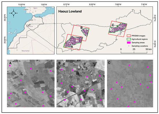
Figure 1.
Location of the study sites in southern Morocco within the Haouz plain. PRISMA images used to cover the three investigated areas: (A) Mejjat; (B) West N’fis; and (C) Central Haouz.
The Haouz plain has been an important experimental setting for investigating a wide range of typical agronomically relevant topics, including soil characterization in arid and semi-arid environments [29,30]. This study was carried out in three agricultural sites (Mejjat, West N’fis, and Central Haouz) (Figure 1) of the Haouz plain, where three PRISMA hyperspectral images were acquired during the no-growing season (June to August), when the bare soil coverage was considered maximal.
The texture of soil varies from loamy sand clay loam to sandy clay, with sand accounting for the majority of it [31]. It has an alkaline pH ranging from 8.1 to 8.78 and a soil organic matter concentration ranging from 0.5 to 2.32% [31]. The soil’s TN distribution of concentrations is detailed in Figure 2.
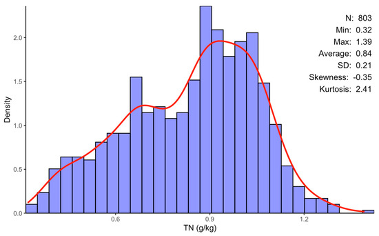
Figure 2.
Summary of descriptive statistics for extracted soil TN content within the Haouz plain: n is the number of samples, Min and Max represent the minimal and the maximal value of the sample, respectively, and SD its standard deviation.
With an average annual precipitation of 250 mm, the study area has a semi-arid continental climate with temperatures ranging from 6 °C in January to 37 °C in August. The winter months (November to April) get the majority of the investigated area’s precipitation (November to April) [30].
2.2. Soil Total Nitrogen Data Mining
In this study, a dataset of 803 samples was generated from open-access soil property and nutrient maps for Africa at a 30 m resolution (i.e., Innovated Solutions for Decision Agriculture, referred to here after as ISDA soil maps). These African digital soil maps were recently made available [24] and include soil data for all of Africa [32]. More details on how the ISDA soil maps were generated are provided by [24]. The locations of the 803 points were chosen across three distinct agricultural sites based on a random stratified method and based on specific criteria: (i) the minimum distance between the samples is 1 km (corresponding to an approximate of 3 × 3 pixels on PRISMA imagery) and (ii) the sampling locations had to fall inside agricultural bare field sites. This selection aimed to ensure a high TN variability in the dataset and, therefore, the robustness of the results. The soil TN contents were then extracted at each of the 803 locations from the ISDA soil layer. The same dataset (803 sampling points) was stacked over the three hyperspectral imageries. To avoid any georeferencing errors between the PRISMA images and the ISDA soil map, each of the 803 samples belonged to a distinct parcel (Figure 1A–C), with each covering a 90 × 90 m square buffer area to obtain homogeneous soil-type samples. To account for any positioning errors, we considered synthetic elementary sampling units (ESUs) with three times the dimensions of the PRISMA sensor spatial resolution [33]. This consideration was achieved through a 3 × 3 cell buffer (1 ha area) that was around each sample point, for which TN values from the 9 cells were extracted and averaged. The values of TN had to be transformed to be converted from a logarithmic scale to g/kg (N) K using the equations prescribed by the map provider as follows:
where is the soil values in field units (g/kg) and y is the raw map soil nutrient values represented in logarithmic scale. Equation (1) was provided from [24].
TN (g/kg) = e(y/100)
2.3. PRISMA Hyperspectral Imagery Acquisition and Processing
In this study, we used three archived cloud-free hyperspectral PRISMA images that were acquired on 12 July 2020 and 2 June and 28 August 2021 over the three investigated sites, as shown in Figure 1. It is important to note that the number of the current PRISMA images over Moroccan agricultural land remain very rare, so the availability of PRISMA images was the primary criterion behind our choice of the investigated sites. Another motivation behind using three images is to have a substantially higher number of sampling locations to train and validate our models. These three images were chosen to capture the agricultural area of each of the three sites, so that the data contains reflectance values from bare soil. The fallow area of the agricultural areas was captured in the images, ensuring that the data only comprises reflectance values from bare soil when determining the best bands for TN characterization. Using the “PRISMAread” R tool, the pictures were integrated into a single raster cube. [34]. Each image has a spatial resolution of 30 m and is composed of 231 small bands with an average spectral resolution of 10 nm or less in the spectral range of 400 to 2500 nm, with overlapped narrow bands between 920 and 1010 nm (Figure 3). The sheer amount of water vapor in the environment caused substantial signal absorption, as evidenced by the spectral data along two regions (1338–1449 nm and 1793–1993 nm). Due to this restriction, twenty-six bands were not considered in our analysis [35]. Further image enhancements were carried out before coupling the ISDA soil map measurements of the soil TN to PRISMA spectral reflectance information, because the first three images were not correctly aligned with the ground data. This was most likely because of a geocoding error brought on by a shift in the ground control point network at the time of the image capture [36]. Therefore, using georeferenced Sentinel 2 pictures that captured the identical regions, we carried out a geometrical correction by image-to-image orthorectification. Reflectance spectra were smoothed using Savitzky–Golay polynomial convolution to reduce the effects of high-frequency random noise, baseline drift, uneven samples, and light scattering and to amplify weak signals. This filter is a mean filter smoothing, and the new value for the midpoint is determined by averaging the spectral reflectance values of all the points inside the selected window (Figure 3) [37]. The used equation is expressed as follows:
where (number of sampling points) is the size of the filter, and is the index of the midpoint. represents the new value of the window’s midpoint. The broader the filter window, the smoother the outcome, but this also increases the odds of losing useful granular spectral information. For this investigation, an optimum filter window size of five was used to establish a balance between these two attributes.
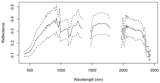
Figure 3.
Soil sample spectra representing the mean TN content after adjustments over the research area. The dotted lines represent the hyperspectral dataset’s variation. The significant signal absorption by the atmosphere in two locations (1338–1449 nm and 1793–1993 nm) owes to the existence of moisture vapor in those specific spectral regions.
To link the PRISMA reflectance information from each of the 803 locations to the ISDA soil map, the same 3 × 3 buffer was used to create a soil spectral information dataset from each of the three hyperspectral images. The resulting mean of the spectral signatures of the 803 samples (i.e., black curve) are shown in Figure 3 together with their variability (i.e., ±SD).
2.4. Ensemble Learning Model
Considering that soil TN and soil reflectance can interact in a complex nonlinear way [6], using multiple feature selection models is a sensible approach to comprehending these intricate relationships. To analyze the relationship between the soil TN acquired from the ISDA soil map and the related soil reflectance, we used an ensemble learning method consisting of 3 methods: partial least square regression (PLSR) [38], support vector regression (SVR) [39], and Gaussian process regression (GPR) [40]. It is crucial to note that the three methods were combined, compared in terms of significant bands, and then applied in both the band selection process and the validity assessment. For estimating soil properties, PLSR has frequently been applied [41,42,43]. This parametric model was developed with the idea that the dependent variable can be estimated using a linear combination of variables [44] while considering the projections of the dependent and explanatory variables with the aim of maximizing the covariance between projections [44]. Latent vectors—linear combinations of the original bands—were used to address the collinearity among the spectral data (i.e., latent vectors [43]). Using the standard equation and the soil reflectance dataset (n = 803), we estimated the soil parameters in our study:
where y is the target variable and a vector containing each soil TN value, is a predictor variable representing the soil reflectance in bands from 1 to N = 205, is the error vector, and represents the estimated weighted regression coefficients. To make the links between output–predictors simpler, latent variables were introduced. A 10-fold cross-validation was used to update the latent vectors for the soil TN concentrations, and the model only saves the latent vectors with the lowest RMSE.
Since GPR is a nonparametric model, we also included it in our ensemble technique. This model assigns a score to the important traits (i.e., bands) that were taken from the input spectral data [45]. Additionally, GPR makes it possible to assess the relative importance of each band to the model, commenting on the model’s development and explicability. In our work, the GPR model creates a relationship between the output soil TN content, denoted as y, and the soil reflectance at each individual band, indicated as x, such that
where is the training soil reflectance, and K is the kernel function measuring the likelihood between the test spectrum and all N training reflectance responses, and is the weight assigned to the training soil reflectance. A scaled Gaussian kernel function was used:
where is a scaling factor, B is the number of bands, and aims to represent the variance of the relations for each band. By optimizing the marginal likelihood in the training set, we can ensure an optimization of the model parameters (, ) and weights [46]. It is important to mention that the multimethod ensemble scheme was based on a previous study that assessed the hyperspectral response of soil organic carbon [20]. Thus, the three models (i.e., PLS, GPR, and SVR) were employed in parallel, and each of them produced statistical output values (i.e., regression coefficient and variable importance) indicating the most important specific spectral bands for TN prediction. The produced band importance values were merged and converted to an ensemble assessment. Therefore, bands with high influence in all three models gained a high ensemble importance and were considered important. The product of the three weighted importance values per band was taken as the ensemble importance; however, a band must be considered important by all three methods (i.e., PLS, GPR, and SVR) to enter the ensemble.
2.5. Model Performance Assessment
To control the band selection and outcome variable significance ranking in this study, an ensemble model including PLSR, SVR, and GPR was used, with a 10-fold cross-validation to examine how well the ensemble model predicted the soil TN. The root-mean-square error (RMSE) and coefficient of determination (R2), which were calculated from Equations (6) and (7), were used to assess the performance of the ensemble models that were produced.
where n is the total number of samples, and is the difference between the vector of predicted values and the observed values.
2.6. Total Nitrogen Specific Band Selection
We evaluated the spectral bands that the ensemble chose for estimating the TN concentrations based on the significant coefficients derived from each component regressed in the ensemble. Since the latent vectors for PLSR are just linear combinations of the original bands, they allow for a simple interpretation of the model and allow for the direct determination of band-related regression coefficients [25]. In contrast to PLSR, SVR does not directly evaluate the pertinent bands. As a result, the literature specifies several techniques for determining whether spectral areas in SVR models are relevant [47].
This study employed a significant criterion based on the spectral band product and the vector, including the support vectors. According to [48,49], these numbers can be understood in the same way as the regression coefficients. The coefficients’ signs indicate whether a relationship can be positive or negative. In GPR, the low values of tell the training function K that a particular band b has greater information content. The optimized weights indicate how far a band is relevant. A flowchart of the technique followed in this investigation is shown in Figure 4.
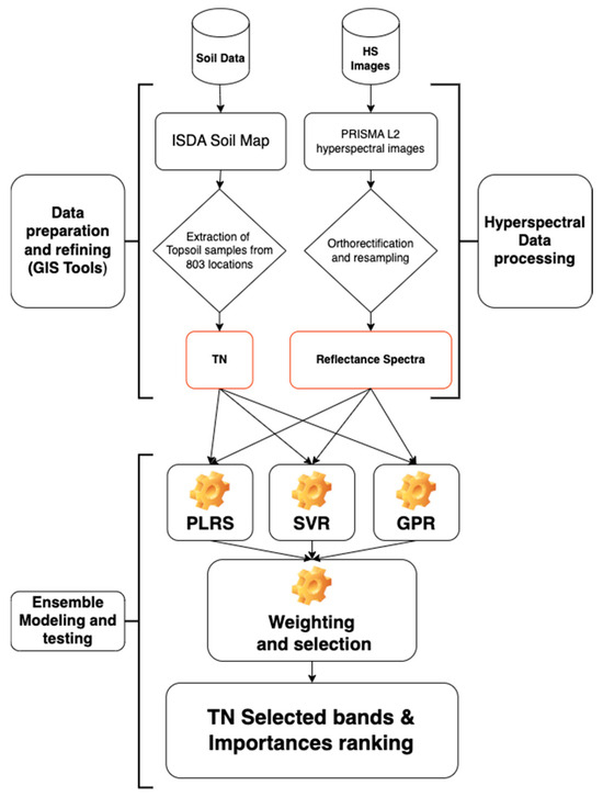
Figure 4.
Diagram illustrating the datasets that were used and the ensemble method that was used to create the relationship between the soil TN dataset and the PRISMA hyperspectral photography dataset. Three learners made up the ensemble method: PLSR (partial least square regression), SVR (support vector regression), and GPR (Gaussian process regression).
3. Results
3.1. Selection of Spectral Bands Specific to Total Nitrogen in Soil
For the 803 analyzed samples, the TN content varied from 0.32 to 1.39 g/kg, with an average value of 0.84 g/kg and a standard deviation (SD) of ±0.21. The ensemble modeling approach used in this study was successful in identifying several spectral bands in the VNIR and SWIR ranges, allowing for estimations of the soil TN contents of the 803 studied samples. Indeed, 27 spectral bands were selected and identified, as shown in Table 1. Most of these selected bands are in the spectral ranges of around 1228–1349 and 1975–2069 nm.

Table 1.
Important bands characterizing soil TN contents selected by the multimethod ensemble approach.
Figure 5 depicts the weighted coefficients of the aggregated method in the ensemble, PLSR, SVR, and GPR, over the wavelength spectrum. It emphasizes the significance of each spectral band in measuring the soil total nitrogen (TN). The PLSR model has substantial variation in its weighted coefficients, indicating the presence of major bands in the ranges of 500–600 nm, 900–1300 nm, and 1900–2100 nm. The SVR model exhibits significant variations, attributing significant importance to bands, especially between the ranges of 500–700 nm, 1400–1600 nm, and 2000–2200 nm. The GPR model, on the other hand, exhibits a more refined and uninterrupted fluctuation, emphasizing significant spectral ranges at around 700–1000 nm and 1200–1300 nm. The ensemble approach aggregates these outcomes, with black shading denoting significant bands and yellow highlights the chosen bands. This integrative approach leverages the strengths of each individual model, ensuring a comprehensive and robust band selection.
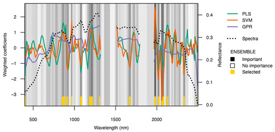
Figure 5.
The coefficients of PLS, SVR, and GPR that were used as measurements of band relevance within the ensemble. Importance was determined by the coefficients of PLS, SVR, and GPR for the relationship between topsoil reflectance and soil TN. The black–white gradients depict the relative significance of each spectral band, while the respective selected bands are marked in yellow.
The spectral bands highlighted by each individual method included in the ensemble are depicted in Figure 5. The GPR concentrated its selection in the region between 1240 and 1349 nm, whereas the PLSR and SVR were all very selective in considering finer regions over the whole spectrum (i.e., 400–2500 nm), particularly at 1000, 478, and 2069 nm, respectively.
Regarding the soil TN content, the PLSR and SVR both performed consistently well, as shown in Table 2. However, the ensemble selection followed a pattern that was more like that of PLSR and GPR than SVR selection, which only comprised bands in the near-infrared (NIR) or SWIR spectrum, respectively. These bands can be found at 739, 749, and within the range of 1228 to 1349 nm.
Table 2.
Ensemble learners fit quantified R2 in 10-fold cross-validation (PLSR and SVR and GPR) for TN.
The most identified specific bands or regions of TN were found at 969, 1078, 1207, 1217, 1975, 1984, 2019, 2061, 2069, and 2077 nm. These findings are consistent with other studies which found that important spectral bands for predicting the soil TN are identified at 1413 and 2207 nm [50]; at 1702, 1870, and 2052 nm [16,17]; from 1800 to 2300 nm; and at 1400 nm, 1900 nm, and 2200 nm. [51,52]. These findings are aligned with previous studies [53] that have reported the potential of an ensemble learner for the selection of spectral bands or regions associated with TN contents for different remote sensing applications. Thus, some of the bands specific to TN in soil that were found in this study agree with the absorption features of TN reported in the literature, whereas others have not been reported before.
3.2. Model Fitting and Spectral Band/Region Selection
The model goodness of fit achieved by the ensemble learners is displayed in Table 2. In most cases, the R2 values obtained with SVR models were the highest. The PLSR and GPR models all achieved similar fits within the ensemble. In general, the models that estimated the TN in the ensemble had values of the coefficient of determination of R2 = 0.63. This demonstrates how well the reflectance levels of the variables’ characteristic band can explain the variation in soil TN concentration. In addition to the coefficient of determination, the distribution of the root-mean-square error (RMSE) resulting from each cross-validation trial was evaluated as a measure of the standard deviation of the unexplained variance by the hyperspectral reflectance (Figure 5). The average RMSE for the component learners of the ensemble model is 0.12 g/kg. In every case, the SVR model had the lowest RMSE values, while the PLSR models had the highest RMSE values. This is consistent with the level of variability explained by the R2 score.
Figure 6 displays the scatter plot comparing the measured versus predicted soil total nitrogen (TN) levels using PLSR, SVR, and GPR. The data points are represented by different colored symbols from one fold of a 10-fold cross-validation process. In this particular fold, the PLSR model on a hand shows a moderate spread around the 1:1 line, indicating reasonable accuracy but with noticeable deviations at higher TN levels. The GPR model aligns closely across lower and mid-range TN levels, though there are slight deviations at higher TN levels. The SVR model on the other hand demonstrates the tightest clustering around the identity line, indicating high precision and consistency across the entire range of TN levels among the previous models.
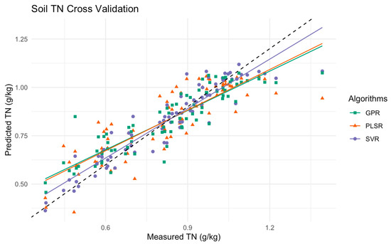
Figure 6.
Scatter plot of measured versus predicted soil TN levels using PLSR, SVR, and GPR models in the multimethod ensemble. This plot represents data that resulted in one-fold from a 10-fold cross-validation, with the black dashed line indicating the ideal 1:1 relationship between measured and predicted values.
4. Discussion
This study aimed to identify a standardized range of spectral bands that can accurately quantify the total nitrogen (TN) content in cropland topsoil using an ensemble learner approach. Our findings indicate that ensemble modeling, integrating PLSR, SVR, and GPR, can effectively identify spectral bands related to the soil TN content. The ensemble model achieved coefficients of determination (R2) values from 0.84, root-mean-square error (RMSE) values from 0.08 g/kg, as well as a robust ratio of performance to deviation (RPD) of 2.53, showcasing its potential for operational soil TN assessments. The goodness of fit metrics found in this study were as high as other studies [54,55] in the literature. The ensemble approach highlighted specific spectral bands in the ranges of 900–1300 nm and 1900–2200 nm. Recent studies have confirmed that it is possible to accurately estimate the soil TN using an aggregation of multi-source optical remote sensing data [56,57,58] and specifically from proximal VNIR spectroscopy [59,60,61]. These regions appear in line with some of the feature importance revealed in different settings in the literature, in which wavebands around 2065, 2071, 2443, 1447.5, 2444.5, and 2443.5 nm were identified using the LUCAS soil spectral library [62] and with bands of around 1520 nm, 1861 nm, 2100 nm, 2286 nm, and 2387 nm that were selected using real-time NIR spectroscopy [63]. Compared to these studies that exclusively deployed in situ spectra, while we find that they highlight different specific wavelengths, all the characteristic wavelengths that we highlighted in our approach appear in similar areas in NIR and SWIR, which demonstrate the capability of PRISMA hyperspectral signals capturing absorption features related to the soil TN. Moreover, previous studies revealed that the wavelength of approximately 1000 nm is related to Fe [64], whereas wavebands of around 940 nm, 1100, and 1350 nm are sensitive wavelengths of soil organic matter (SOM) [65,66], and absorption bands in the SWIR are caused by overtone and combination modes of N and C groups. TN is widely known to have a strong relationship with SOM. This is because of the fact that organic nitrogen reserves are crucial for the provision of accessible nitrogen to crops [67,68]. To verify this claim, we used a soil organic carbon (SOC) layer from the same dataset from which SOM contents were then extracted for every point in our study area. A correlation analysis of our dataset revealed a strong correlation between OM and TN in the area, as illustrated in Figure 7.
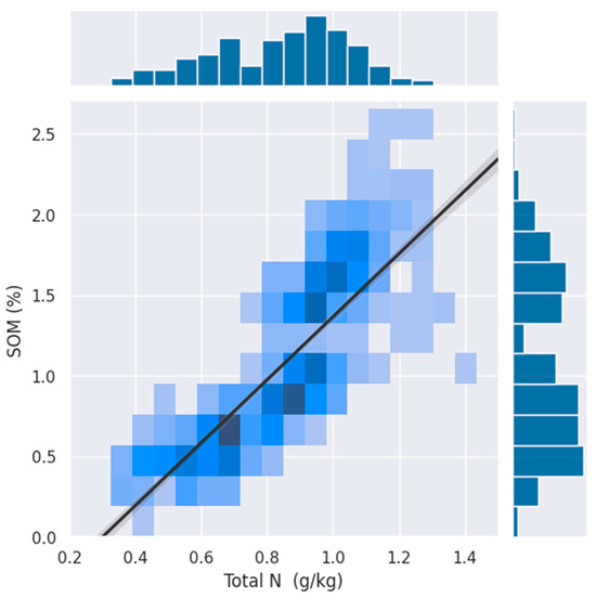
Figure 7.
Relationship between the percentage of the total nitrogen (TN) content (g/kg) and soil organic matter (SOM) in soil samples. The density of the points is indicated by the color intensity, with darker shades of blue representing higher densities of observations. A strong positive correlation is observed, as illustrated by the trend line, suggesting that higher levels of organic matter are associated with an increased total nitrogen content.
Despite the similarities described above, some discrepancies were identified in terms of some specific absorption features, which could be attributed to different reasons. For instance, the hyperspectral signal in our dataset was derived from a spaceborne sensor signal, which was subject to alterations because of the acquisition geometry, as well as noise that incurs while traveling through the atmosphere. On the other hand, the soil TN dataset was sampled from a spatially predicted map with 30 m resolution over the entire African continent and over Morocco with a relatively low number of samples used to calibrate and validate the ISDA soil map near our study area. Yet, it is unclear how accurate current TN soil map predictions of the ISDA maps are. As of today, no study has conducted an evaluation of the site-specific accuracy of the ISDA regional-to-global soil maps over Morocco. For instance, the authors of [69] conducted a study to evaluate both the relative and functional accuracy of ISDA soil maps over Ghana and found that in most cases, these map products are not accurate enough to inform site-specific soil management. This is not surprising given that the TN values we extracted from the ISDA maps are relatively higher to what it is conventionally found in agricultural soils in nearby regions [70]. It is important to note that the ISDA is still one of the rare available soil maps of Africa. It is important to mention that for these studies, accurate information on the TN soil is critical for identifying the management practices needed to improve crop yields. To improve the robustness and applicability of our findings, it is necessary to address several critical areas. Initially, it is imperative to validate the data with a higher resolution. The precision of our model and its usefulness in site-specific soil management could be substantially enhanced by the integration of higher resolution data. Subsequently, it is imperative to conduct an exhaustive uncertainty assessment of the ISDA soil dataset. Although the latest version incorporates higher-resolution Sentinel 2 data and a two-scale modeling approach, these improvements do not completely eliminate uncertainties, and, consequently, the absolute accuracy of the ISDA maps at local scales, particularly in regions such as Morocco, remain unverified. Therefore, to facilitate more informed decision making, it is necessary to evaluate the uncertainty associated with these maps in order to comprehend their limitations and potential errors. Furthermore, the performance of our approach could be improved by contemplating alternative data sources, which could provide additional insights. Combining data from a variety of sources, including local soil surveys, other remote sensing products, and citizen science initiatives at a wider scale, particularly over the north of Africa, can result in a more comprehensive soil profile and reduce dependence on a single dataset. These procedures are essential for the enhancement of soil TN estimation and the subsequent promotion of sustainable agricultural practices. Ultimately, future research should explore the application of this method in diverse regions and with other soil properties. Incorporating additional data sources and experimenting with different machine learning techniques could further enhance model accuracy. Additionally, integrating this approach with drone-based hyperspectral imaging could offer more flexibility and practicality for large-scale agricultural monitoring. In conclusion, our study presents a viable method for soil TN estimation using PRISMA hyperspectral imagery and ensemble learning models. The identified spectral bands and model accuracy underscore the potential of this approach for practical applications in precision agriculture. Further research and technological advancements could enhance the robustness and applicability of this method, contributing to sustainable agricultural practices.
5. Conclusions
In this study, we aimed to establish a standardized range of spectral bands that can accurately quantify the TN content in cropland topsoil using an ensemble learner of of three models (PLS, SVR, and GPR). Some of the selected bands or band regions are like those reported in the literature. Other individual bands or band regions were identified in this study for the first time. This study has also shown that ensemble modeling can conduct operational and quantitative examinations of spectrum signals in relation to the TN soil content. For instance, the ensemble model achieved an R2 ranging from 0.63 to 0.73 and RMSE values from 0.11 to 0.14 g/kg for the single learners, being boosted to an R2 of 0.84, an RMSE of 0.08 g/kg, and an RPD of 2.53, Notably, some of the selected bands are comparable with those reported in the literature, demonstrating the ability of PRISMA imagery to capture specific absorption features similar to those identified using in situ proximal spectroscopy. These findings carry significant implications for the development of precise, cost-effective agricultural management tools, especially for smallholder farmers in Africa. The ensemble learning model’s ability to discern specific spectral bands for TN suggests that remote sensing can be effectively utilized for soil nutrient management, potentially transforming the UAV industry by informing the creation of new, optimized TN-specific sensors. While the results are promising, the performance of the ensemble model and the accuracy of the ISDA soil map predictions used warrant further investigation. Subsequent validations with higher-resolution datasets are essential to refine the accuracy of remote soil TN estimation. This research paves the way for enhanced precision in agricultural practices, leveraging the power of spaceborne hyperspectral sensors to enable more informed and sustainable farming decisions. Still, further evaluations of such modeling techniques are required, particularly for field applications employing datasets with a better resolution, which may improve the accuracy of remote soil TN estimation.
Author Contributions
Conceptualization, K.M. and A.L.; formal analysis, K.M.; funding acquisition, A.C.; investigation, A.L.; methodology, K.M. and A.L.; project administration, A.L.; software, K.M.; supervision, A.L., R.C. and A.C.; validation, K.M., A.L. and P.V.; visualization, K.M.; writing—original draft, K.M.; writing—review and editing, K.M., A.L., P.V., K.K., R.C. and A.C. All authors have read and agreed to the published version of the manuscript.
Funding
This project was financially supported by The Yield Gap project (agreement between OCP Foundation and the Mohammed VI Polytechnic University (UM6P) under reference number 135PR007. The lead author received financial support from UM6P.
Data Availability Statement
The data that support the findings of this study is freely supplied by iSDA Soil at https://doi.org/10.5281/zenodo.4090386. Any requests about data should be directed to the iSDA Soil.
Acknowledgments
The authors acknowledge all the technical support of the PI of Yield Gap project. This manuscript was checked for spelling and grammar by the UM6P English language specialist team. We also thank the academic editor and anonymous reviewers for agreeing to review an earlier version of this manuscript.
Conflicts of Interest
The data that support the findings of this study is freely supplied by iSDA Soil at https://doi.org/10.5281/zenodo.4090386 (accessed on 15 April 2024). Any requests about data should be directed to the iSDA Soil.
References
- Saito, K.; Vandamme, E.; Johnson, J.M.; Tanaka, A.; Senthilkumar, K.; Dieng, I.; Akakpo, C.; Gbaguidi, F.; Segda, Z.; Bassoro, I.; et al. Yield-Limiting Macronutrients for Rice in Sub-Saharan Africa. Geoderma 2019, 338, 546–554. [Google Scholar] [CrossRef]
- Lu, H.J.; Ye, Z.Q.; Zhang, X.L.; Lin, X.Y.; Ni, W.Z. Growth and Yield Responses of Crops and Macronutrient Balance Influenced by Commercial Organic Manure Used as a Partial Substitute for Chemical Fertilizers in an Intensive Vegetable Cropping System. Phys. Chem. Earth 2011, 36, 387–394. [Google Scholar] [CrossRef]
- Skjemstad, J.O.; Janik, L.J.; Taylor, J.A. Non-Living Soil Organic Matter: What Do We Know about It? Aust. J. Exp. Agric. 1998, 38, 667–680. [Google Scholar] [CrossRef]
- Viscarra Rossel, R.A.; Walvoort, D.J.J.; McBratney, A.B.; Janik, L.J.; Skjemstad, J.O. Visible, near Infrared, Mid Infrared or Combined Diffuse Reflectance Spectroscopy for Simultaneous Assessment of Various Soil Properties. Geoderma 2006, 131, 59–75. [Google Scholar] [CrossRef]
- Soriano-Disla, J.M.; Janik, L.J.; Viscarra Rossel, R.A.; MacDonald, L.M.; McLaughlin, M.J. The Performance of Visible, near-, and Mid-Infrared Reflectance Spectroscopy for Prediction of Soil Physical, Chemical, and Biological Properties. Appl. Spectrosc. Rev. 2014, 49, 139–186. [Google Scholar] [CrossRef]
- Rossel, R.V. The Soil Spectroscopy Group and the Development of a Global Soil Spectral Library. NIR News 2009, 20, 14–15. [Google Scholar] [CrossRef]
- Ben-Dor, E.; Chabrillat, S.; Demattê, J.A.M.; Taylor, G.R.; Hill, J.; Whiting, M.L.; Sommer, S. Using Imaging Spectroscopy to Study Soil Properties. Remote Sens. Environ. 2009, 113, S38–S55. [Google Scholar] [CrossRef]
- Dunn, B.W.; Beecher, H.G.; Batten, G.D.; Ciavarella, S. The Potential of Near-Infrared Reflectance Spectroscopy for Soil Analysis—A Case Study from the Riverine Plain of South-Eastern Australia. Aust. J. Exp. Agric. 2002, 42, 607–614. [Google Scholar] [CrossRef]
- Malley, D.F.; Yesmin, L.; Eilers, R.G. Rapid Analysis of Hog Manure and Manure-Amended Soils Using Near-Infrared Spectroscopy. Soil Sci. Soc. Am. J. 2002, 66, 1677–1686. [Google Scholar] [CrossRef]
- Cozzolino, D.; Morón, A. The Potential of Near-Infrared Reflectance Spectroscopy to Analyse Soil Chemical and Physical Characteristics. J. Agric. Sci. 2003, 140, 65–71. [Google Scholar] [CrossRef]
- Islam, K.; Singh, B.; McBratney, A. Simultaneous Estimation of Several Soil Properties by Ultra-Violet, Visible, and near-Infrared Reflectance Spectroscopy. Aust. J. Soil Res. 2003, 41, 1101–1114. [Google Scholar] [CrossRef]
- Lee, W.S.; Sanchez, J.F.; Mylavarapu, R.S.; Choe, J.S. Estimating Chemical Properties of Florida Soils Using Spectral Reflectance. Trans. Am. Soc. Agric. Eng. 2003, 46, 1443–1453. [Google Scholar] [CrossRef]
- Jiang, W.; Liu, X.; Wang, Y.; Zhang, Y.; Qi, W. Responses to Potassium Application and Economic Optimum K Rate of Maize under Different Soil Indigenous K Supply. Sustainability 2018, 10, 2267. [Google Scholar] [CrossRef]
- Wenjun, J.; Zhou, S.; Jingyi, H.; Shuo, L. In Situ Measurement of Some Soil Properties in Paddy Soil Using Visible and Near-Infrared Spectroscopy. PLoS ONE 2014, 9, e105708. [Google Scholar] [CrossRef]
- He, Y.; Huang, M.; García, A.; Hernández, A.; Song, H. Prediction of Soil Macronutrients Content Using Near-Infrared Spectroscopy. Comput. Electron. Agric. 2007, 58, 144–153. [Google Scholar] [CrossRef]
- Dalal, R.C.; Henry, R.J. Simultaneous Determination of Moisture, Organic Carbon, and Total Nitrogen by Near Infrared Reflectance Spectrophotometry. Soil Sci. Soc. Am. J. 1986, 50, 120–123. [Google Scholar] [CrossRef]
- Ehsani, M.R.; Upadhyaya, S.K.; Slaughter, D.; Shafii, S.; Pelletier, M. A NIR Technique for Rapid Determination of Soil Mineral Nitrogen. Precis. Agric. 1999, 1, 217–234. [Google Scholar] [CrossRef]
- Ben-Dor, E.; Banin, A. Near-Infrared Analysis as a Rapid Method to Simultaneously Evaluate Several Soil Properties. Soil Sci. Soc. Am. J. 1995, 59, 364–372. [Google Scholar] [CrossRef]
- Shepherd, K.D.; Walsh, M.G. Development of Reflectance Spectral Libraries for Characterization of Soil Properties. Soil Sci. Soc. Am. J. 2002, 66, 988–998. [Google Scholar] [CrossRef]
- Laamrani, A.; Berg, A.A.; Voroney, P.; Feilhauer, H.; Blackburn, L.; March, M.; Dao, P.D.; He, Y.; Martin, R.C. Ensemble Identification of Spectral Bands Related to Soil Organic Carbon Levels over an Agricultural Field in Southern Ontario, Canada. Remote Sens. 2019, 11, 1298. [Google Scholar] [CrossRef]
- Mzid, N.; Castaldi, F.; Tolomio, M.; Pascucci, S.; Casa, R.; Pignatti, S. Evaluation of Agricultural Bare Soil Properties Retrieval from Landsat 8, Sentinel-2 and PRISMA Satellite Data. Remote Sens. 2022, 14, 714. [Google Scholar] [CrossRef]
- Andersen, C.M.; Bro, R. Variable Selection in Regression—A Tutorial. J. Chemom. 2010, 24, 728–737. [Google Scholar] [CrossRef]
- Genuer, R.; Poggi, J.M.; Tuleau-Malot, C. Variable Selection Using Random Forests. Pattern Recognit. Lett. 2010, 31, 2225–2236. [Google Scholar] [CrossRef]
- Hengl, T.; Miller, M.A.E.; Križan, J.; Shepherd, K.D.; Sila, A.; Kilibarda, M.; Antonijević, O.; Glušica, L.; Dobermann, A.; Haefele, S.M.; et al. African Soil Properties and Nutrients Mapped at 30 m Spatial Resolution Using Two-Scale Ensemble Machine Learning. Sci. Rep. 2021, 11, 6130. [Google Scholar] [CrossRef] [PubMed]
- Wold, S.; Sjöström, M.; Eriksson, L. PLS-Regression: A Basic Tool of Chemometrics. In Proceedings of the Chemometrics and Intelligent Laboratory Systems; Elsevier: Amsterdam, The Netherlands, 2001; Volume 58, pp. 109–130. [Google Scholar]
- Ustin, S.L.; Gitelson, A.A.; Jacquemoud, S.; Schaepman, M.; Asner, G.P.; Gamon, J.A.; Zarco-Tejada, P. Retrieval of Foliar Information about Plant Pigment Systems from High Resolution Spectroscopy. Remote Sens. Environ. 2009, 113, S67–S77. [Google Scholar] [CrossRef]
- Du, P.; Xia, J.; Chanussot, J.; He, X. Hyperspectral Remote Sensing Image Classification Based on the Integration of Support Vector Machine and Random Forest. In Proceedings of the International Geoscience and Remote Sensing Symposium (IGARSS), Munich, Germany, 22–27 July 2012; pp. 174–177. [Google Scholar]
- Duchemin, B.; Hadria, R.; Erraki, S.; Boulet, G.; Maisongrande, P.; Chehbouni, A.; Escadafal, R.; Ezzahar, J.; Hoedjes, J.C.B.; Kharrou, M.H.; et al. Monitoring Wheat Phenology and Irrigation in Central Morocco: On the Use of Relationships between Evapotranspiration, Crops Coefficients, Leaf Area Index and Remotely-Sensed Vegetation Indices. Agric. Water Manag. 2006, 79, 1–27. [Google Scholar] [CrossRef]
- Khabba, S.; Jarlan, L.; Er-Raki, S.; Le Page, M.; Ezzahar, J.; Boulet, G.; Simonneaux, V.; Kharrou, M.H.; Hanich, L.; Chehbouni, G. The SudMed Program and the Joint International Laboratory TREMA: A Decade of Water Transfer Study in the Soil-Plant-Atmosphere System over Irrigated Crops in Semi-Arid Area. Procedia Environ. Sci. 2013, 19, 524–533. [Google Scholar] [CrossRef]
- Ouassanouan, Y.; Fakir, Y.; Simonneaux, V.; Kharrou, M.H.; Bouimouass, H.; Najar, I.; Benrhanem, M.; Sguir, F.; Chehbouni, A. Multi-Decadal Analysis of Water Resources and Agricultural Change in a Mediterranean Semiarid Irrigated Piedmont under Water Scarcity and Human Interaction. Sci. Total Environ. 2022, 834, 155328. [Google Scholar] [CrossRef] [PubMed]
- Sefiani, S.; El Mandour, A.; Laftouhi, N.-E.; Khalil, N.; Kamal, S.; Jarlan, L.; Chehbouni, A.; Hanich, L.; Khabba, S.; Hamaoui, A. Assessment of Soil Quality for a Semi-Arid Irrigated Under Citrus Orchard: Case of the Haouz Plain, Morocco. Eur. Sci. J. 2017, 13, 367. [Google Scholar] [CrossRef][Green Version]
- Miller, M.A.E.; Shepherd, K.D.; Kisitu, B.; Collinson, J. ISDAsoil: The First Continent-Scale Soil Property Map at 30 m Resolution Provides a Soil Information Revolution for Africa. PLoS Biol. 2021, 19, e3001441. [Google Scholar] [CrossRef]
- Marshall, M.; Thenkabail, P. Advantage of Hyperspectral EO-1 Hyperion over Multispectral IKONOS, GeoEye-1, WorldView-2, Landsat ETM+, and MODIS Vegetation Indices in Crop Biomass Estimation. ISPRS J. Photogramm. Remote Sens. 2015, 108, 205–218. [Google Scholar] [CrossRef]
- Busetto, L. Lbusett/Prismaread: Prismaread v0.2.0; Zenodo: Genève, Switzerland, 2020. [Google Scholar] [CrossRef]
- Marshall, M.; Thenkabail, P. Biomass Modeling of Four Leading World Crops Using Hyperspectral Narrowbands in Support of HyspIRI Mission. Photogramm. Eng. Remote Sens. 2014, 80, 757–772. [Google Scholar] [CrossRef]
- Marshall, M.; Belgiu, M.; Boschetti, M.; Pepe, M.; Stein, A.; Nelson, A. Field-Level Crop Yield Estimation with PRISMA and Sentinel-2. ISPRS J. Photogramm. Remote Sens. 2022, 187, 191–210. [Google Scholar] [CrossRef]
- Savitzky, A.; Golay, M.J.E. Smoothing and Differentiation of Data by Simplified Least Squares Procedures. Anal. Chem. 1964, 36, 1627–1639. [Google Scholar] [CrossRef]
- Mevik, B.H.; Wehrens, R. The Pls Package: Principal Component and Partial Least Squares Regression in R. J. Stat. Softw. 2007, 18, 1–23. [Google Scholar] [CrossRef]
- Karatzoglou, A.; Hornik, K.; Smola, A.; Zeileis, A. Kernlab—An S4 Package for Kernel Methods in R. J. Stat. Softw. 2004, 11, 1–20. [Google Scholar] [CrossRef]
- Williams, C.K.I.; Barber, D. Bayesian Classification with Gaussian Processes. IEEE Trans. Pattern Anal. Mach. Intell. 1998, 20, 1342–1351. [Google Scholar] [CrossRef]
- Aldabaa, A.A.A.; Weindorf, D.C.; Chakraborty, S.; Sharma, A.; Li, B. Combination of Proximal and Remote Sensing Methods for Rapid Soil Salinity Quantification. Geoderma 2015, 239, 34–46. [Google Scholar] [CrossRef]
- Yu, H.; Liu, M.; Du, B.; Wang, Z.; Hu, L.; Zhang, B. Mapping Soil Salinity/Sodicity by Using Landsat OLI Imagery and PLSR Algorithm over Semiarid West Jilin Province, China. Sensors 2018, 18, 1048. [Google Scholar] [CrossRef]
- Minu, S.; Shetty, A.; Gopal, B. Review of Preprocessing Techniques Used in Soil Property Prediction from Hyperspectral Data. Cogent Geosci. 2016, 2, 1145878. [Google Scholar] [CrossRef]
- Wang, F.; Gao, J.; Zha, Y. Hyperspectral Sensing of Heavy Metals in Soil and Vegetation: Feasibility and Challenges. ISPRS J. Photogramm. Remote Sens. 2018, 136, 73–84. [Google Scholar] [CrossRef]
- Erler, A.; Riebe, D.; Beitz, T.; Löhmannsröben, H.G.; Gebbers, R. Soil Nutrient Detection for Precision Agriculture Using Handheld Laser-Induced Breakdown Spectroscopy (LIBS) and Multivariate Regression Methods (PLSR, Lasso and GPR). Sensors 2020, 20, 418. [Google Scholar] [CrossRef] [PubMed]
- Rasmussen, C.E. Gaussian Processes in Machine Learning. Lect. Notes Comput. Sci. 2004, 3176, 63–71. [Google Scholar] [CrossRef]
- Macabiog, R.E.N.; Fadchar, N.A.; Cruz, J.C. Dela Soil NPK Levels Characterization Using Near Infrared and Artificial Neural Network. In Proceedings of the 2020 16th IEEE International Colloquium on Signal Processing & Its Applications (CSPA), Langkawi, Malaysia, 28–29 February 2020; pp. 141–145. [Google Scholar]
- Axelsson, C.; Skidmore, A.K.; Schlerf, M.; Fauzi, A.; Verhoef, W. Hyperspectral Analysis of Mangrove Foliar Chemistry Using PLSR and Support Vector Regression. Int. J. Remote Sens. 2013, 34, 1724–1743. [Google Scholar] [CrossRef]
- Üstün, B.; Melssen, W.J.; Buydens, L.M.C. Visualisation and Interpretation of Support Vector Regression Models. Anal. Chim. Acta 2007, 595, 299–309. [Google Scholar] [CrossRef] [PubMed]
- Kawamura, K.; Tsujimoto, Y.; Rabenarivo, M.; Asai, H.; Andriamananjara, A.; Rakotoson, T. Vis-NIR Spectroscopy and PLS Regression with Waveband Selection for Estimating the Total C and N of Paddy Soils in Madagascar. Remote Sens. 2017, 9, 1081. [Google Scholar] [CrossRef]
- Dinakaran, J.; Bidalia, A.; Kumar, A.; Hanief, M.; Meena, A.; Rao, K.S. Near-Infrared-Spectroscopy for Determination of Carbon and Nitrogen in Indian Soils. Commun. Soil Sci. Plant Anal. 2016, 47, 1503–1516. [Google Scholar] [CrossRef]
- Chacón Iznaga, A.; Rodríguez Orozco, M.; Aguila Alcantara, E.; Carral Pairol, M.; Díaz Sicilia, Y.E.; de Baerdemaeker, J.; Saeys, W. Vis/NIR Spectroscopic Measurement of Selected Soil Fertility Parameters of Cuban Agricultural Cambisols. Biosyst. Eng. 2014, 125, 105–121. [Google Scholar] [CrossRef]
- Stenberg, B.; Viscarra Rossel, R.A.; Mouazen, A.M.; Wetterlind, J. Visible and Near Infrared Spectroscopy in Soil Science. Adv. Agron. 2010, 107, 163–215. [Google Scholar] [CrossRef]
- Wang, Y.; Li, M.; Ji, R.; Wang, M.; Zheng, L. Comparison of Soil Total Nitrogen Content Prediction Models Based on Vis-NIR Spectroscopy. Sensors 2020, 20, 7078. [Google Scholar] [CrossRef]
- Feng, Y.; Li, X.; Wang, W.; Liu, C. Detection of Soil Total Nitrogen by Vis-SWNIR Spectroscopy. In Proceedings of the IFIP Advances in Information and Communication Technology; Springer New York LLC: New York, NY, USA, 2011; Volume 347, pp. 184–191. [Google Scholar]
- Zhang, Q.; Liu, M.; Zhang, Y.; Mao, D.; Li, F.; Wu, F.; Song, J.; Li, X.; Kou, C.; Li, C.; et al. Comparison of Machine Learning Methods for Predicting Soil Total Nitrogen Content Using Landsat-8, Sentinel-1, and Sentinel-2 Images. Remote Sens. 2023, 15, 2907. [Google Scholar] [CrossRef]
- Zhang, Y.; Sui, B.; Shen, H.; Ouyang, L. Mapping Stocks of Soil Total Nitrogen Using Remote Sensing Data: A Comparison of Random Forest Models with Different Predictors. Comput. Electron. Agric. 2019, 160, 23–30. [Google Scholar] [CrossRef]
- Xu, Y.; Smith, S.E.; Grunwald, S.; Abd-Elrahman, A.; Wani, S.P.; Nair, V.D. Estimating Soil Total Nitrogen in Smallholder Farm Settings Using Remote Sensing Spectral Indices and Regression Kriging. Catena 2018, 163, 111–122. [Google Scholar] [CrossRef]
- Debaene, G.; Bartmiński, P.; Siłuch, M. In Situ VIS-NIR Spectroscopy for a Basic and Rapid Soil Investigation. Sensors 2023, 23, 5495. [Google Scholar] [CrossRef] [PubMed]
- Clingensmith, C.M.; Grunwald, S. Predicting Soil Properties and Interpreting Vis-NIR Models from across Continental United States. Sensors 2022, 22, 3187. [Google Scholar] [CrossRef] [PubMed]
- Zhou, P.; Li, M.; Yang, W.; Yao, X.; Liu, Z.; Ji, R. Development and Performance Tests of an On-the-Go Detector of Soil Total Nitrogen Concentration Based on near-Infrared Spectroscopy. Precis. Agric. 2021, 22, 1479–1500. [Google Scholar] [CrossRef]
- Wang, Y.; Li, M.; Ji, R.; Wang, M.; Zheng, L. A Deep Learning-Based Method for Screening Soil Total Nitrogen Characteristic Wavelengths. Comput. Electron. Agric. 2021, 187, 106228. [Google Scholar] [CrossRef]
- Zhang, Y.; Li, M.; Zheng, L.; Zhao, Y.; Pei, X. Soil Nitrogen Content Forecasting Based on Real-Time NIR Spectroscopy. Comput. Electron. Agric. 2016, 124, 29–36. [Google Scholar] [CrossRef]
- Palacios-Orueta, A.; Ustin, S.L. Remote sensing of soil properties in the Santa Monica Mountains I. Spectral analysis. Remote Sens. Environ. 1998, 65, 170–183. [Google Scholar] [CrossRef]
- Kweon, G.; Maxton, C. Soil Organic Matter Sensing with an On-the-Go Optical Sensor. Biosyst. Eng. 2013, 115, 66–81. [Google Scholar] [CrossRef]
- Daniel, K.W.; Tripathi, N.K.; Honda, K.; Apisit, E. Analysis of VNIR (400–1100 Nm) Spectral Signatures for Estimation of Soil Organic Matter in Tropical Soils of Thailand. Int. J. Remote Sens. 2004, 25, 83–91. [Google Scholar] [CrossRef]
- Farzadfar, S.; Knight, J.D.; Congreves, K.A. Soil Organic Nitrogen: An Overlooked but Potentially Significant Contribution to Crop Nutrition. Plant Soil 2021, 462, 7–23. [Google Scholar] [CrossRef] [PubMed]
- Yan, M.; Pan, G.; Lavallee, J.M.; Conant, R.T. Rethinking Sources of Nitrogen to Cereal Crops. Glob. Chang. Biol. 2020, 26, 191–199. [Google Scholar] [CrossRef] [PubMed]
- Maynard, J.J.; Yeboah, E.; Owusu, S.; Buenemann, M.; Neff, J.C.; Herrick, J.E. Accuracy of Regional-to-Global Soil Maps for on-Farm Decision-Making: Are Soil Maps “Good Enough”? SOIL 2023, 9, 277–300. [Google Scholar] [CrossRef]
- John, K.; Bouslihim, Y.; Isong, I.A.; Hssaini, L.; Razouk, R.; Kebonye, N.M.; Agyeman, P.C.; Penížek, V.; Zádorová, T. Mapping Soil Nutrients via Different Covariates Combinations: Theory and an Example from Morocco. Ecol. Process 2022, 11, 23. [Google Scholar] [CrossRef]


Disclaimer/Publisher’s Note: The statements, opinions and data contained in all publications are solely those of the individual author(s) and contributor(s) and not of MDPI and/or the editor(s). MDPI and/or the editor(s) disclaim responsibility for any injury to people or property resulting from any ideas, methods, instructions or products referred to in the content. |
© 2024 by the authors. Licensee MDPI, Basel, Switzerland. This article is an open access article distributed under the terms and conditions of the Creative Commons Attribution (CC BY) license (https://creativecommons.org/licenses/by/4.0/).