
Ensemble Learning for the Land Cover Classification of Loess Hills in the Eastern Qinghai–Tibet Plateau Using GF-7 Multitemporal Imagery


Abstract

1. Introduction
2. Study Area and Data Sources
2.1. Research Area
2.2. Data and Preprocessing
2.2.1. GF-7 Images and Preprocessing
2.2.2. DEM Production Based on a GF-7 Stereo Image Pair
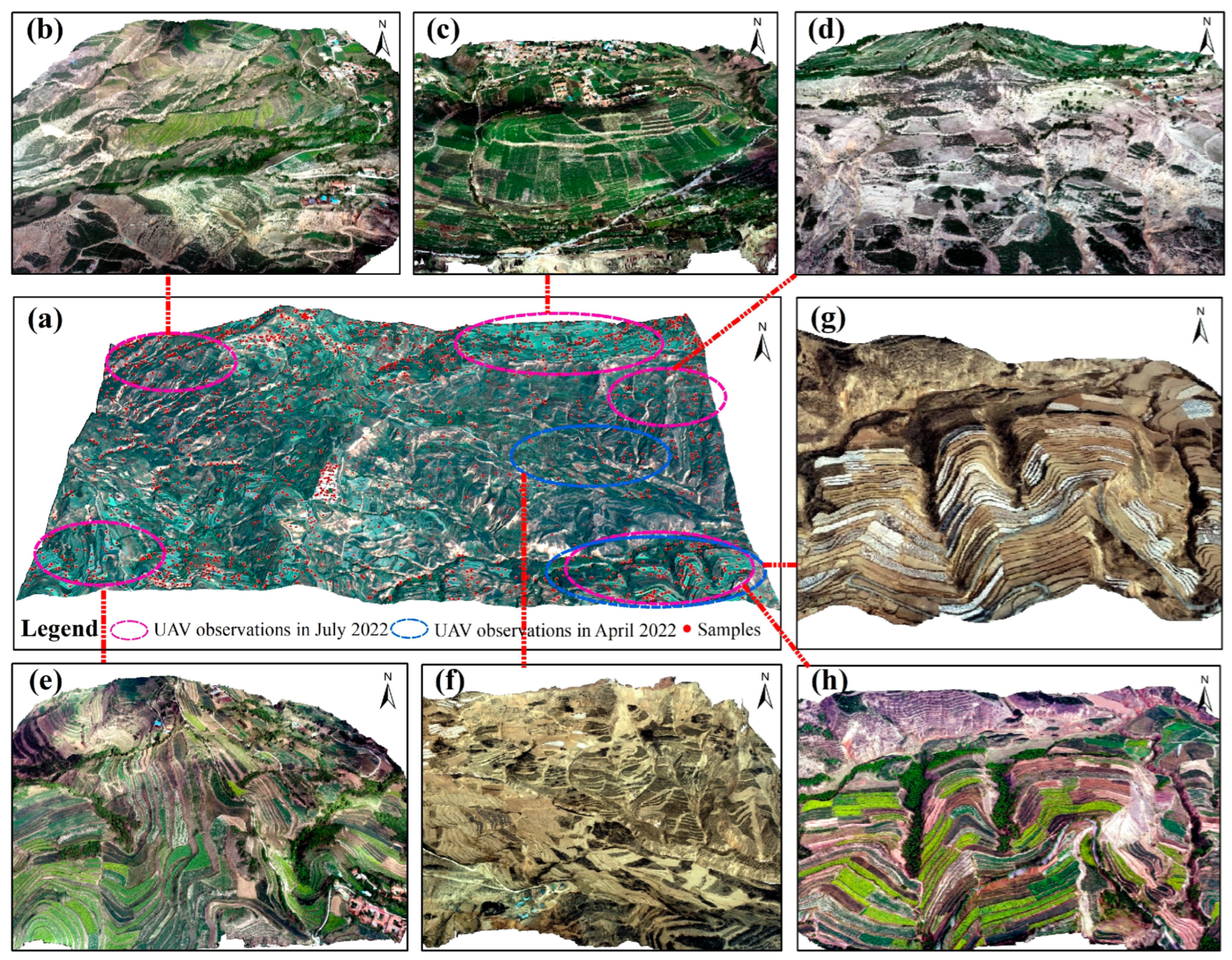
2.2.3. UAV Images and Preprocessing
2.2.4. Classification Sample Data
2.2.5. Classification System
3. Methods
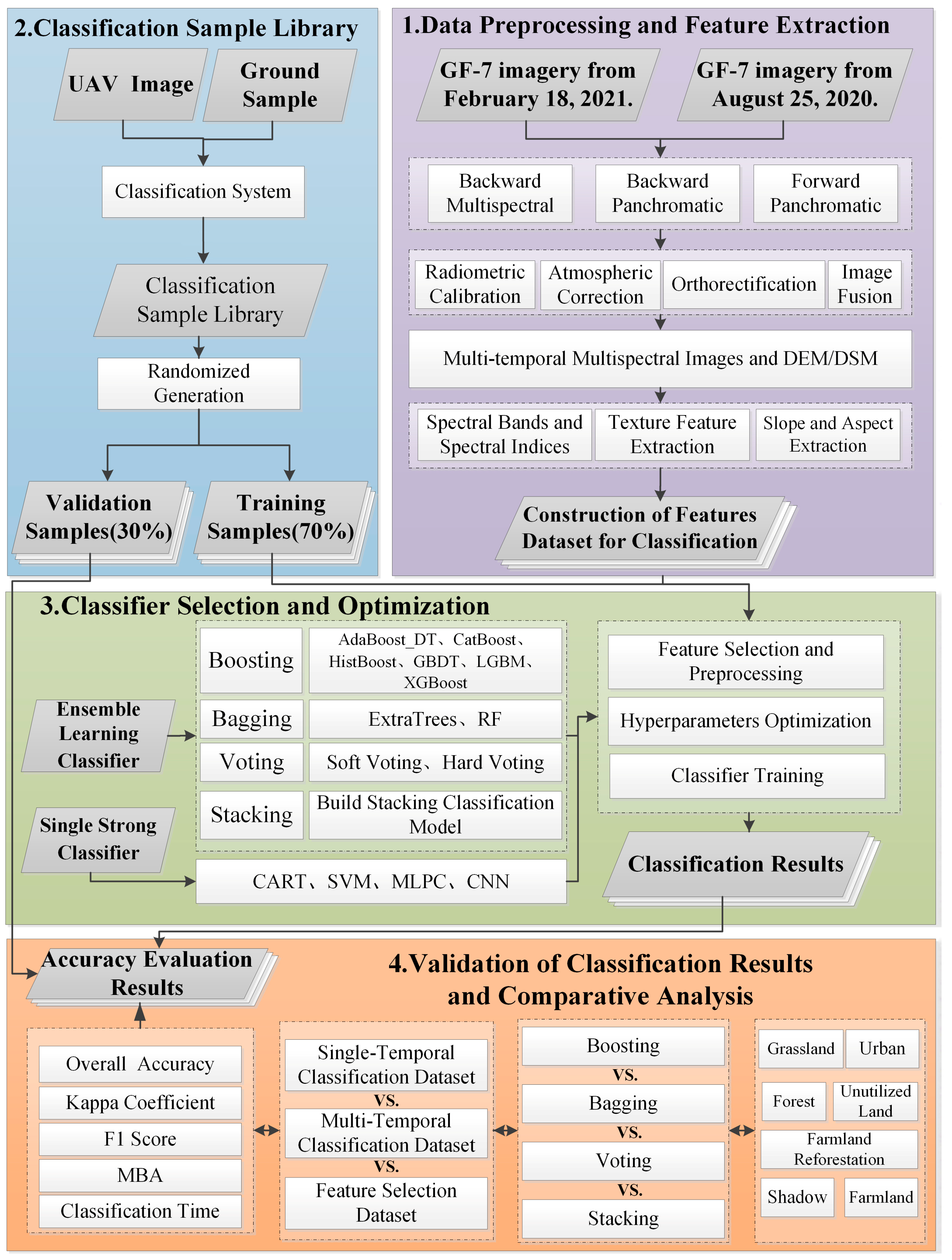
3.1. Overview
3.2. Classifiers
3.2.1. Bagging
3.2.2. Boosting
3.2.3. Stacking
3.2.4. Voting
3.2.5. Single Strong Classifier
3.3. Classification Feature Extraction and Optimization
3.4. Classification Dataset Construction
3.5. Accuracy Evaluation Metrics
4. Classification Results and Accuracy Evaluation
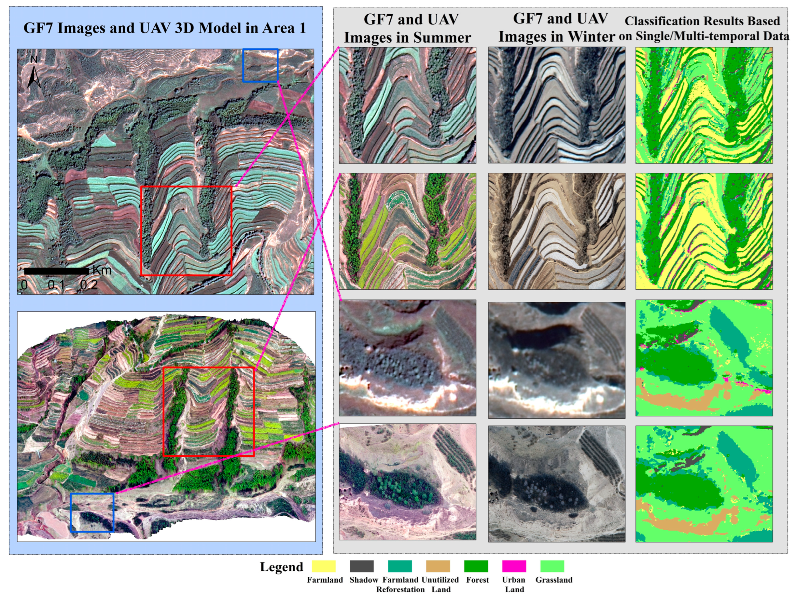
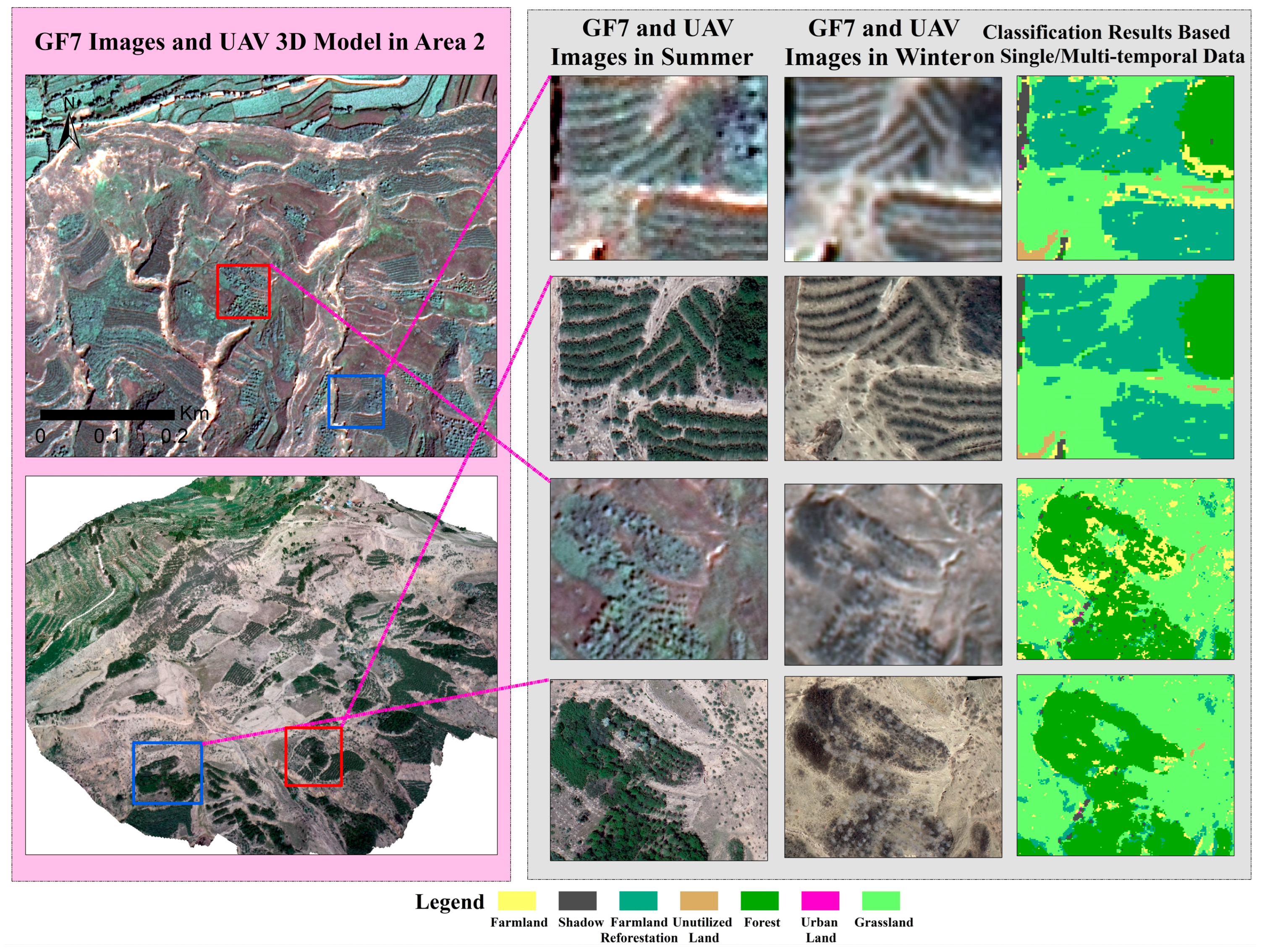
4.1. Classification Results
4.2. Accuracy Evaluation
4.2.1. Evaluation of the Classification Accuracy Using Single-Temporal Data
4.2.2. Evaluation of the Classification Accuracy Using Multitemporal Data
4.3. Classification Feature Optimization and Classification Accuracy Evaluation
4.3.1. Evaluation of Classification Feature Importance and Feature Optimization
4.3.2. Classification Results and Accuracy Evaluation after Classification Feature Optimization
5. Discussion
5.1. Impact of the Classifier on the Classification Results
5.1.1. Comparison of the Overall Accuracies of the Classifiers
5.1.2. Comparison of the Differences in the Recognition Accuracy of the Specific Ground Features by Classifier
5.2. Effect of Classification Data on Separability and the Classification Results of Ground Features
5.2.1. Effect of Classification Datasets on the Classification Accuracy
5.2.2. Effect of Classification Datasets on the Separability of Land Types
5.2.3. Impact of Classification Datasets on Classification Time
5.3. Limitations and Future Work
6. Conclusions
- (1)
- Compared with the accuracies of the CART, SVM, and MLP traditional single classifiers, the accuracies of the 11 ensemble learning classifiers were superior across all three land cover classification datasets. Using ensemble learning classifiers could introduce a 5% to 9% improvement in the accuracy of LULC classification for the study area. For the same classification dataset, the difference in accuracy indicators between the 11 ensemble learning classifiers was generally 1–3%. HistGBoost, LightGBM, and other boosting classifiers that adopted techniques such as histogram processing performed better in terms of accuracy. The performance of the bagging classifier was robust, while the accuracy of the ExtraTrees classifier was better. Stacking improved the overall accuracy of the classifier more significantly relative to its member classifiers than voting.
- (2)
- Compared with the land cover classification accuracies when using the feature optimization and single-temporal datasets, the land cover classification accuracy achieved by each classifier on the multitemporal dataset was better. The differences in accuracy indicators achieved using different classification datasets with the same classifier were generally 1–3%. Using multitemporal datasets could greatly improve differentiation among forestland returned from farmland, grassland, and forestland, which helps to improve the overall classification accuracy.
- (3)
- Classification features such as the NIR-S, DEM, mean, RRI-S, Green-S, and SAVI-W were optimized more times, contributing to the performance of each classifier. Each ensemble classifier reduced the time spent on classification after the feature optimization of the multitemporal dataset, and AdaBoost-DT, stacking, and ExtraTrees maintained a better classification accuracy.
- (4)
- Based on a comprehensive consideration of the accuracy evaluation results of each classifier, the GF-7 satellite data were confirmed to have good applicability in the land cover classification of complex topographic areas and can provide data support for the accurate identification of land cover types in loess hills and similar topographic areas.
Author Contributions
Funding
Data Availability Statement
Acknowledgments
Conflicts of Interest
References
- Camilleri, S.; De Giglio, M.; Stecchi, F.; Pérez-Hurtado, A. Land use and land cover change analysis in predominantly man-made coastal wetlands: Towards a methodological framework. Wetl. Ecol. Manag. 2017, 25, 23–43. [Google Scholar] [CrossRef]
- Defries, R. Terrestrial vegetation in the coupled human-earth system: Contributions of remote sensing. Ann. Rev. Environ. Resour. 2008, 33, 369–390. [Google Scholar] [CrossRef]
- Gong, P.J.; Wang, J.; Yu, L.; Zhao, Y.; Zhao, Y.; Liang, L.; Niu, Z.; Huang, X.; Fu, H.; Liu, S.; et al. Finer resolution observation and monitoring of global land cover: First mapping results with Landsat TM and ETM+ data. Int. J. Remote Sens. 2013, 34, 2607–2654. [Google Scholar] [CrossRef]
- Zhou, Y.; Liu, F.; Zhang, G.; Wang, J. Response of the Normalized Difference Vegetation Index (NDVI) to Snow Cover Changes on the Qinghai–Tibet Plateau. Remote Sens. 2024, 16, 2140. [Google Scholar] [CrossRef]
- Sun, H.; Zheng, D.; Yao, T.; Zhang, Y. Protection and construction of the national ecological security shelter zone on Tibetan Plateau. Acta Geogr. Sin. 2012, 67, 3–12. [Google Scholar]
- Zhang, Y.; Liu, L.; Wang, Z.; Bai, W.; Ding, M.; Wang, X. Spatial and temporal characteristics of land use and cover changes in the Tibetan Plateau. Chin. Sci. Bull. 2019, 64, 2865–2875. [Google Scholar]
- Liu, Z.; Liu, S.; Qi, W.; Jin, H. The settlement intention of floating population and the factors in Qinghai-Tibet Plateau: An analysis from the perspective of short-distance and long-distance migrants. Acta Geogr. Sin. 2022, 76, 1907–1919. [Google Scholar]
- Shi, F.; Zhou, B.; Zhou, H.; Zhang, H.; Li, H.; Li, R.; Guo, Z.; Gao, X. Spatial Autocorrelation Analysis of Land Use and Ecosystem Service Value in the Huangshui River Basin at the Grid Scale. Plants 2022, 11, 2294. [Google Scholar] [CrossRef] [PubMed]
- Tang, M. Land Use/Land Cover Information Extraction from SPOT6 Imagery with Object-Oriented and Random Forest Methods in the Huangshui River Basin. Master’s Thesis, Qinghai Normal University, Xining, China, 2020. [Google Scholar]
- Li, J. Research on Land Use/Land Cover Classification in Complex Terrain Areas. Master’s Thesis, Qinghai Normal University, Xining, China, 2013. [Google Scholar]
- Jia, W. Research on Object-Oriented Land Use Information Extraction in Complex Terrain Areas. Master’s Thesis, Qinghai Normal University, Xining, China, 2015. [Google Scholar]
- Gu, X. Research on Land Use/Land Cover Classification in Huangshui Basin Based on Machine Learning. Master’s Thesis, Qinghai Normal University, Xining, China, 2018. [Google Scholar]
- Ma, H. Land Use/Land Cover Change Detection in Huangshui River Basin Based on Random Forest. Master’s Thesis, Qinghai Normal University, Xining, China, 2018. [Google Scholar]
- Shen, Z. Land Use/Land Cover Classification and Accuracy Assessment in Huangshui Basin Based on GEE’s Landsat Image Long-Term Series Data. Master’s Thesis, Qinghai Normal University, Xining, China, 2020. [Google Scholar]
- Li, R. Research on Land Cover Classification Based on Ensemble Learning—A Case Study of the Huangshui River Basin in the Northeast of Qinghai-Tibet Plateau. Master’s Thesis, Qinghai Normal University, Xining, China, 2020. [Google Scholar]
- Cui, K.; Li, R.; Polk, S.L.; Lin, Y.; Zhang, H.; Murphy, J.M.; Plemmons, R.J.; Chan, R.H. Superpixel-based and Spatially-regularized Diffusion Learning for Unsupervised Hyperspectral Image Clustering. IEEE Trans. Geosci. Remote Sens. 2024, 5, 4. [Google Scholar] [CrossRef]
- Maung, W.S.; Tsuyuki, S.; Guo, Z. Improving Land Use and Land Cover Information of Wunbaik Mangrove Area in Myanmar Using U-Net Model with Multisource Remote Sensing Datasets. Remote Sens. 2024, 16, 76. [Google Scholar] [CrossRef]
- Lam, C.-N.; Niculescu, S.; Bengoufa, S. Monitoring and Mapping Floods and Floodable Areas in the Mekong Delta (Vietnam) Using Time-Series Sentinel-1 Images, Convolutional Neural Network, Multi-Layer Perceptron, and Random Forest. Remote Sens. 2023, 15, 2001. [Google Scholar] [CrossRef]
- Li, H.; Gao, X.; Tang, M. Research on land cover classification of images with different spatial resolutions based on CNN. Remote Sens. Technol. Appl. 2020, 35, 749–758. [Google Scholar]
- Li, H. Research on Land Cover Classification of Sentinel-2 Multi-Seasonal Data Based on Gradient Boosting Tree and Random Forest. Master’s Thesis, Qinghai Normal University, Xining, China, 2021. [Google Scholar]
- Hao, T.; Elith, J.; Lahoz-Monfort, J.J.; Guillera-Arroita, G. Testing whether ensemble modelling is advantageous for maximising predictive performance of species distribution models. Ecography 2020, 43, 549–558. [Google Scholar] [CrossRef]
- Luo, H.; Li, M.; Dai, S.; Li, H.; Li, Y.; Hu, Y.; Zheng, Q.; Yu, X.; Fang, J. Combinations of Feature Selection and Machine Learning Algorithms for Object-Oriented Betel Palms and Mango Plantations Classification Based on Gaofen-2 Imagery. Remote Sens. 2022, 14, 1757. [Google Scholar] [CrossRef]
- Kohavi, R.; Provost, F. Glossary of terms: Machine learning. Appl. Mach. Learn. Knowl. Discov. Process 1998, 30, 271. [Google Scholar]
- Wen, L.; Hughes, M. Coastal Wetland Mapping Using Ensemble Learning Algorithms: A Comparative Study of Bagging, Boosting and Stacking Techniques. Remote Sens. 2020, 12, 1683. [Google Scholar] [CrossRef]
- Castillo-Navarro, J.; Saux, B.L.; Boulch, A.; Audebert, N.; Lefèvre, S. Semi-Supervised Semantic Segmentation in Earth Observation: The MiniFrance Suite, Dataset Analysis and Multi-Task Network Study. Mach. Learn. 2022, 111, 3125–3160. [Google Scholar] [CrossRef]
- Cuypers, S.; Nascetti, A.; Vergauwen, M. Land Use and Land Cover Mapping with VHR and Multi-Temporal Sentinel-2 Imagery. Remote Sens. 2023, 15, 2501. [Google Scholar] [CrossRef]
- Xie, G.; Niculescu, S. Mapping and Monitoring of Land Cover/Land Use (LCLU) Changes in the Crozon Peninsula (Brittany, France) from 2007 to 2018 by Machine Learning Algorithms (Support Vector Machine, Random Forest, and Convolutional Neural Network) and by Post-classification Comparison (PCC). Remote Sens. 2021, 13, 3899. [Google Scholar] [CrossRef]
- Sánchez, A.-M.S.; González-Piqueras, J.; de la Ossa, L.; Calera, A. Convolutional Neural Networks for Agricultural Land Use Classification from Sentinel-2 Image Time Series. Remote Sens. 2022, 14, 5373. [Google Scholar] [CrossRef]
- Kroupi, E.; Kesa, M.; Navarro-Sánchez, V.D.; Saeed, S.; Pelloquin, C.; Alhaddad, B.; Moreno, L.; Soria-Frisch, A.; Ruffini, G. Deep convolutional neural networks for land-cover classification with Sentinel-2 images. J. Appl. Remote Sens. 2019, 13, 024525. [Google Scholar] [CrossRef]
- Polikar, R. Ensemble based systems in decision making. IEEE Circuits Syst. 2006, 6, 21–45. [Google Scholar] [CrossRef]
- Zhou, Z.H. Ensemble Methods: Foundations and Algorithms; CRC Press: Boca Raton, FL, USA; London, UK; New York, NY, USA, 2012. [Google Scholar]
- Qinghai Provincial Bureau of Statistics. Qinghai Statistical Yearbook 2020; China Statistics Press: Beijing, China, 2020; pp. 1–23. [Google Scholar]
- Li, Z.; Chen, Z.; Cheng, Q.; Duan, F.; Sui, R.; Huang, X.; Xu, H. UAV-Based Hyperspectral and Ensemble Machine Learning for Predicting Yield in Winter Wheat. Agronomy 2022, 12, 202. [Google Scholar] [CrossRef]
- Liu, J.; Kuang, W.; Zhang, Z.; Xu, X.; Qin, Y.; Ning, J.; Chi, W. Spatiotemporal characteristics, patterns, and causes of land-use changes in China since the late 1980s. J. Geogr. Sci. 2014, 24, 195–210. [Google Scholar] [CrossRef]
- Chan, J.C.W.; Huang, C.; DeFries, R. Enhanced algorithm performance for land cover classification from remotely sensed data using bagging and boosting. IEEE Trans. Geosci. Remote Sens. 2001, 39, 693–695. [Google Scholar]
- Ahn, J.M.; Kim, J.; Kim, K. Ensemble Machine Learning of Gradient Boosting (XGBoost, LightGBM, CatBoost) and Attention-Based CNN-LSTM for Harmful Algal Blooms Forecasting. Toxins 2023, 15, 608. [Google Scholar] [CrossRef] [PubMed]
- Van der Laan, M.J.; Polley, E.C.; Hubbard, A.E. Super learner. Stat. Appl. Genet. Mol. Biol. 2007, 6, 9. [Google Scholar] [CrossRef] [PubMed]
- Shuai, S.; Zhang, Z.; Zhang, T.; Luo, W.; Tan, L.; Duan, X.; Wu, J. Innovative Decision Fusion for Accurate Crop/Vegetation Classification with Multiple Classifiers and Multisource Remote Sensing Data. Remote Sens. 2024, 16, 1579. [Google Scholar] [CrossRef]
- El-Naqa, I.; Yang, Y.; Wernick, M.N.; Galatsanos, N.P.; Nishikawa, R.M. A Support Vector Machine Approach for Detection of Microcalcifications. IEEE Trans. Med. 2002, 21, 1552–1563. [Google Scholar] [CrossRef] [PubMed]
- Pontil, M.; Verri, A. Support Vector Machines for 3d Object Recognition. IEEE Trans. Pattern Anal. Mach. Intell. 1998, 6, 637–646. [Google Scholar] [CrossRef]
- Ren, J.; Wang, R.; Liu, G.; Wang, Y.; Wu, W. An SVM-Based Nested Sliding Window Approach for Spectral-Spatial Classification of Hyperspectral Images. Remote Sens. 2021, 13, 114. [Google Scholar] [CrossRef]
- Hsu, C.W.; Lin, C.J. A Comparison of Methods for Multiclass Support Vector Machines. IEEE Trans. Neural Netw. 2002, 13, 415–425. [Google Scholar] [PubMed]
- Chan, R.H.; Li, R. A 3-Stage Spectral-Spatial Method for Hyperspectral Image Classification. Remote Sens. 2022, 14, 3998. [Google Scholar] [CrossRef]
- Cheng, F.; Ou, G.; Wang, M.; Liu, C. Remote Sensing Estimation of Forest Carbon Stock Based on Machine Learning Algorithms. Forests 2024, 15, 681. [Google Scholar] [CrossRef]
- Breiman, L.; Friedman, J.H.; Olshen, R. Classification and Regression Trees; Routledge: London, UK, 2017. [Google Scholar]
- Peña-Barragán, J.M.; Ngugi, M.K.; Plant, R.E.; Six, J. Object-based crop identification using multiple vegetation indices, textural features and crop phenology. Remote Sens. Environ. 2011, 115, 1301–1316. [Google Scholar] [CrossRef]
- Reschke, J.; Christian, H. Continuous field mapping of Mediterranean wetlands using sub-pixel spectral signatures and multi-temporal Landsat data. Int. J. Appl. Earth Obs. Geoinf. 2014, 28, 220–229. [Google Scholar]
- Haralick, R.M.; Shanmugam, K.S. Combined spectral and spatial processing of ERTS imagery data. Remote Sens. Environ. 1974, 3, 3–13. [Google Scholar] [CrossRef]
- Padhee, S.K.; Dutta, S. Spatio-Temporal Reconstruction of MODIS NDVI by Regional Land Surface Phenology and Harmonic Analysis of Time-Series. GISci. Remote Sens. 2019, 56, 1261–1288. [Google Scholar]
- Laliberte, A.S.; Browning, D.M.; Rango, A. A comparison of three feature selection methods for object-based classification of sub-decimeter resolution Ultra Cam-L imagery. Int. J. Appl. Earth Obs. 2012, 15, 70–78. [Google Scholar]
- Ferri, C.; Hernández-Orallo, J.; Modroiu, R. An experimental comparison of performance measures for classification. Pattern Recognit. Lett. 2009, 30, 27–38. [Google Scholar] [CrossRef]
- Wang, D.; Huo, Z.; Miao, P.; Tian, X. Comparison of Machine Learning Models to Predict Lake Area in an Arid Area. Remote Sens. 2023, 15, 4153. [Google Scholar] [CrossRef]
- Peppes, N.; Daskalakis, E.; Alexakis, T.; Adamopoulou, E.; Demestichas, K. Performance of Machine Learning-Based Multi-Model Voting Ensemble Methods for Network Threat Detection in Agriculture 4.0. Sensors 2021, 21, 7475. [Google Scholar] [CrossRef] [PubMed]
- Kpienbaareh, D.; Sun, X.; Wang, J.; Luginaah, I.; Bezner Kerr, R.; Lupafya, E.; Dakishoni, L. Crop Type and Land Cover Mapping in Northern Malawi Using the Integration of Sentinel-1, Sentinel-2, and PlanetScope Satellite Data. Remote Sens. 2021, 13, 700. [Google Scholar] [CrossRef]
- Arrechea-Castillo, D.A.; Solano-Correa, Y.T.; Muñoz-Ordóñez, J.F.; Pencue-Fierro, E.L.; Figueroa-Casas, A. Multiclass Land Use and Land Cover Classification of Andean Sub-Basins in Colombia with Sentinel-2 and Deep Learning. Remote Sens. 2023, 15, 2521. [Google Scholar] [CrossRef]
- Cheng, K.; Scott, G.J. Deep Seasonal Network for Remote Sensing Imagery Classification of Multi-Temporal Sentinel-2 Data. Remote Sens. 2023, 15, 4705. [Google Scholar] [CrossRef]
- Vanniel, T.; McVicar, T.; Datt, B. On the relationship between training sample size and data dimensionality: Monte Carlo analysis of broadband multi-temporal classification. Remote Sens. Environ. 2005, 98, 468–480. [Google Scholar] [CrossRef]
- Ajibola, S.; Cabral, P. A Systematic Literature Review and Bibliometric Analysis of Semantic Segmentation Models in Land Cover Mapping. Remote Sens. 2024, 16, 2222. [Google Scholar] [CrossRef]
- Nasiri, V.; Darvishsefat, A.A.; Arefi, H.; Griess, V.C.; Sadeghi, S.M.; Borz, S.A. Modeling Forest Canopy Cover: A Synergistic Use of Sentinel-2, Aerial Photogrammetry Data, and Machine Learning. Remote Sens. 2022, 14, 1453. [Google Scholar] [CrossRef]


| Image Thumbnail | Date Acquired | Image Type | Spatial Resolution (m) | Spectral Ranges (μm) | Cloud Cover (%) |
|---|---|---|---|---|---|
 | 25 August 2020 | Backward multispectral | 2.6 | B1 0.45–0.52 | 0 |
| B2 0.52–0.59 | |||||
| B3 0.63–0.69 | |||||
 | 8 February 2021 | B4 0.77–0.89 | |||
| Backward panchromatic | 0.65 | 0.45–0.9 | |||
| Forward panchromatic | 0.8 |
| Land Cover Types | Description | True-Color Composite Image of GF-7 Satellite on 25 August 2020 | False-Color Composite Image of GF-7 Satellite on 25 August 2020 | True-Color Composite Image of GF-7 Satellite on 18 February 2021 | True-Color Composite Image of Unmanned Aerial Vehicle in 2021 |
|---|---|---|---|---|---|
| Urban land | Urban construction land and urban roads | 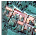 |  |  |  |
| Forestland | Shrubs and woodlands | 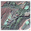 |  | 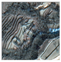 |  |
| Farmland reforestation | Forest land returned from farmland |  |  |  |  |
| Farmland | Cultivated land in loess hilly region |  |  |  | 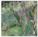 |
| Cultivated land in flat terrain |  |  | 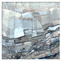 | 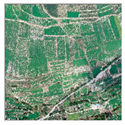 | |
| Grassland | Grassland loess hilly region |  | 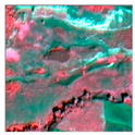 |  |  |
| Unutilized land | Bare land |  |  |  | 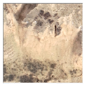 |
| Shadow | Shadows from forested and built-up areas | 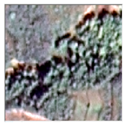 |  |  |  |
| Classifiers | Parameters | Description | Tuning Ranges |
|---|---|---|---|
| HistGBoost, LGBM, AdaBoost_DT, CatBoost, XGBoost, GBDT, and CNN | learning_rate | The learning rate, controlling the update magnitude of model parameters in each iteration. | 0.01–0.3 |
| HistGBoost, LGBM, XGBoost, GBDT, RF, ExtraTrees, and CART | max_depth | The maximum depth of each tree. | 1–50 |
| LGBM, AdaBoost_DT, XGBoost, GBDT, RF, and ExtraTrees | n_estimators | The number of trees, representing the number of iterations. | 1–300 |
| HistGBoost, RF, ExtraTrees, CART, and GBDT | min_samples_leaf | The minimum number of samples a leaf node must have. | 1–20 |
| HistGBoost, RF, ExtraTrees, CART, and GBDT | min_samples_split | The minimum number of samples a node must have to be split. | 1–20 |
| XGBoost | min_child_weight | The minimum sum of instance weight in each leaf node. | 1–50 |
| LGBM | boosting_type | The parameter that specifies the type or strategy of the gradient boosting algorithm. | gbdt |
| min_child_samples | The minimum number of samples in each leaf node. | 1–50 | |
| AdaBoost_DT | algorithm | The algorithm implementation for AdaBoost. | SAMME.R, SAMME |
| CatBoost | iterations | The number of iterations, representing the number of boosting rounds. | 1000 |
| depth | Depth of the trees. | 1–50 | |
| loss_function | The parameter used to specify the loss function utilized during the training process. | MultiClass | |
| GBDT | criterion | The parameter used to define the criterion for measuring split quality. | Friedman_mse |
| RF | max_features | The number of features to consider when looking for the best split. | None |
| SVM | kernel | The kernel parameter used to specify the kernel function employed for transforming the input data. | RBF |
| C | The parameter that controls the penalty of misclassification. | 1–100 | |
| MLPC | hidden_layer_sizes | The parameter that specifies the number of neurons in each hidden layer. | 1–100 |
| activation | The parameter that specifies the activation function for the hidden layers. | Relu, Tanh, Logistic | |
| solver | The parameter that specifies the optimization algorithm used for weight optimization. | Adam, Sgd, Lbfgs | |
| max_iter | The number of iterations. | 1500 | |
| CNN | Number of Convolutional Layers | The parameter that determines the depth and complexity of feature extraction. | 9 |
| Kernel Size | The parameter that specifies the spatial extent of each convolutional filter. | 5.3 | |
| Regularization | The parameter used to prevent overfitting | Dropout | |
| Activation Function | The parameter that introduces non-linearity into the model. | Relu |
| Types | Features | Description | References |
|---|---|---|---|
| Summer and winter temporal spectral bands | Blue band | Use the 1st, 2nd, 3rd, and 4th bands of the GF-7 backward multispectral and backward panchromatic spectral fusion images from 25 August 2020 and 18 February 2021 for calculation, with a spatial resolution of 0.68 m. | [46] |
| Green band | |||
| Red band | |||
| NIR band | |||
| Summer and winter temporal spectral indices | Normalized differential vegetation index (NDVI) | Use the 1st, 2nd, 3rd, and 4th bands of the GF-7 backward multispectral and backward panchromatic spectral fusion images from 25 August 2020 and 18 February 2021 for calculation, with enhancement of vegetation, water bodies, and urban areas. | [46] |
| Normalized differential water index (NDWI) | |||
| Ratio of the resident area index (RRI) | |||
| Green vegetation index (VIgreen) | |||
| Soil-adjusted vegetation index (SAVI) | |||
| Enhanced vegetation index (EVI) | |||
| Time series spectral index | Time series normalized vegetation index (NDVI-TS) | Use GF-7 satellite images from summer and winter to calculate the NDVI-TS and EVI-TS. These indices are utilized to assess the vegetation growth variations during different periods. | [47] |
| Time series enhanced vegetation index (EVI-TS) | |||
| Terrain information | DEM | Use the backward and forward panchromatic image of the GF-7 from 25 August 2020 for digital elevation model (DEM) calculation, with a spatial resolution of 0.68 m. Use the DSM for slope, aspect, and shaded relief calculation, with a spatial resolution of 0.68 m, which mainly indicate the topographic information. | [14,20] |
| Slope | |||
| Aspect | |||
| Shaded relief | |||
| Texture information | Mean | After performing the principal component analysis (PCA) on the 1st, 2nd, 3rd, and 4th bands of the GF-7 backward multispectral and backward panchromatic spectral fusion images from 25 August 2020, the first principal component is used to calculate the gray-level cooccurrence matrix (GLCM) to reflect the information on the distance, grayscale level, and direction in the image. | [48,50] |
| Variance | |||
| Homogeneity | |||
| Contrast | |||
| Dissimilarity | |||
| Entropy | |||
| Second moment | |||
| Correlation |
| Types | Features | Number |
|---|---|---|
| Single-temporal classification dataset (-S) | Summer temporal spectral bands (Blue-S, Green-S, Red-S, NIR-S) Summer temporal spectral indices (NDVI-S, NDWI-S, RRI-S, VIgreen-S, SAVI-S, EVI-S) Terrain information (DEM, slope, aspect, shaded relief) Texture information (mean, variance, homogeneity, contrast, dissimilarity, entropy, second moment, correlation) | 22 |
| Multitemporal classification dataset (-M) | Summer temporal spectral bands (Blue-S, Green-S, Red-S, NIR-S) Winter temporal spectral bands (Blue-W, Green-W, Red-W, NIR-W) Summer temporal spectral indices (NDVI-S, NDWI-S, RRI-S, VIgreen-S, SAVI-S, EVI-S) Winter temporal spectral indices (NDVI-W, NDWI-W, RRI-W, VIgreen-W, SAVI-W, EVI-W) Time series spectral index (NDVI-TS, EVI-TS) Terrain information (DEM, slope, aspect, shaded relief) Texture information (mean, variance, homogeneity, contrast, dissimilarity, entropy, second moment, correlation) | 34 |
| Feature selection dataset for classification (-FS) | Automatically select classification features based on the feature importance scoring methods inherent to each classifier | 10–19 |
| Model | Producer Accuracy (PA) | OA | Kappa | MBA | F1- Score | ||||||
|---|---|---|---|---|---|---|---|---|---|---|---|
| Urban | Unutilized Land | Shadow | Farmland Returned to Forest Land | Grassland | Forest | Farmland | |||||
| AdaBoost_DT | 0.89 | 1.00 | 0.97 | 0.92 | 0.84 | 0.90 | 0.89 | 0.904 | 0.882 | 0.910 | 0.905 |
| CART | 0.81 | 0.95 | 0.95 | 0.85 | 0.81 | 0.82 | 0.86 | 0.856 | 0.824 | 0.851 | 0.856 |
| CatBoost | 0.92 | 0.98 | 0.98 | 0.89 | 0.86 | 0.86 | 0.90 | 0.902 | 0.880 | 0.904 | 0.903 |
| CNN | 0.92 | 0.99 | 0.98 | 0.90 | 0.84 | 0.88 | 0.91 | 0.905 | 0.883 | 0.910 | 0.906 |
| ExtraTrees | 0.92 | 1.00 | 0.97 | 0.86 | 0.86 | 0.87 | 0.91 | 0.904 | 0.882 | 0.905 | 0.904 |
| GBDT | 0.94 | 0.96 | 0.98 | 0.90 | 0.87 | 0.89 | 0.87 | 0.900 | 0.878 | 0.901 | 0.902 |
| Hard Voting | 0.98 | 0.96 | 0.96 | 0.89 | 0.81 | 0.92 | 0.87 | 0.896 | 0.872 | 0.903 | 0.897 |
| HistGBoost | 0.89 | 1.00 | 0.97 | 0.92 | 0.84 | 0.90 | 0.89 | 0.907 | 0.886 | 0.916 | 0.908 |
| LGBM | 0.96 | 0.98 | 0.98 | 0.90 | 0.86 | 0.89 | 0.89 | 0.907 | 0.886 | 0.911 | 0.908 |
| MLPC | 0.52 | 0.59 | 0.88 | 0.75 | 0.78 | 0.95 | 0.91 | 0.809 | 0.768 | 0.779 | 0.806 |
| RF | 0.88 | 1.00 | 0.97 | 0.92 | 0.87 | 0.86 | 0.90 | 0.904 | 0.882 | 0.904 | 0.904 |
| Soft Voting | 0.94 | 0.98 | 0.97 | 0.89 | 0.86 | 0.89 | 0.90 | 0.907 | 0.886 | 0.915 | 0.908 |
| Stacking | 0.94 | 0.98 | 0.97 | 0.91 | 0.87 | 0.87 | 0.90 | 0.907 | 0.886 | 0.915 | 0.908 |
| SVM | 0.81 | 0.95 | 0.89 | 0.78 | 0.77 | 0.92 | 0.90 | 0.855 | 0.824 | 0.860 | 0.854 |
| XGBoost | 0.92 | 0.98 | 0.97 | 0.90 | 0.86 | 0.88 | 0.89 | 0.902 | 0.880 | 0.908 | 0.903 |
| Model | Producer Accuracy (PA) | OA | Kappa | MBA | F1- Score | ||||||
|---|---|---|---|---|---|---|---|---|---|---|---|
| Urban | Unutilized Land | Shadow | Farmland Returned to Forest Land | Grassland | Forest | Farmland | |||||
| AdaBoost-DT | 0.96 | 0.96 | 0.97 | 0.89 | 0.87 | 0.92 | 0.96 | 0.933 | 0.918 | 0.933 | 0.933 |
| CART | 0.85 | 0.90 | 0.97 | 0.84 | 0.79 | 0.86 | 0.92 | 0.876 | 0.849 | 0.880 | 0.876 |
| CatBoost | 0.98 | 0.96 | 0.98 | 0.89 | 0.87 | 0.93 | 0.95 | 0.931 | 0.916 | 0.933 | 0.932 |
| CNN | 0.99 | 0.93 | 0.99 | 0.91 | 0.90 | 0.92 | 0.92 | 0.936 | 0.923 | 0.937 | 0.936 |
| ExtraTrees | 0.96 | 0.96 | 0.93 | 0.87 | 0.88 | 0.91 | 0.95 | 0.922 | 0.905 | 0.923 | 0.921 |
| GBDT | 0.96 | 0.98 | 0.97 | 0.86 | 0.88 | 0.92 | 0.95 | 0.928 | 0.912 | 0.931 | 0.928 |
| Hard Voting | 0.96 | 0.96 | 0.96 | 0.89 | 0.86 | 0.95 | 0.93 | 0.922 | 0.905 | 0.919 | 0.921 |
| HistGBoost | 0.98 | 0.94 | 0.97 | 0.89 | 0.90 | 0.93 | 0.95 | 0.935 | 0.920 | 0.937 | 0.935 |
| LGBM | 0.98 | 0.94 | 0.98 | 0.89 | 0.89 | 0.92 | 0.95 | 0.933 | 0.918 | 0.933 | 0.933 |
| MLPC | 0.74 | 0.79 | 0.94 | 0.82 | 0.70 | 0.83 | 0.94 | 0.834 | 0.796 | 0.806 | 0.831 |
| RF | 0.96 | 0.96 | 0.97 | 0.90 | 0.86 | 0.91 | 0.95 | 0.925 | 0.908 | 0.924 | 0.924 |
| Soft Voting | 0.98 | 0.94 | 0.97 | 0.89 | 0.86 | 0.95 | 0.95 | 0.930 | 0.914 | 0.932 | 0.930 |
| Stacking | 0.98 | 0.94 | 0.97 | 0.90 | 0.90 | 0.92 | 0.94 | 0.931 | 0.916 | 0.933 | 0.932 |
| SVM | 0.86 | 1.00 | 0.92 | 0.80 | 0.81 | 0.89 | 0.97 | 0.889 | 0.866 | 0.897 | 0.892 |
| XGBoost | 0.98 | 0.94 | 0.97 | 0.92 | 0.89 | 0.90 | 0.94 | 0.928 | 0.912 | 0.932 | 0.929 |
| Model | Producer Accuracy (PA) | OA | Kappa | MBA | F1- Score | ||||||
|---|---|---|---|---|---|---|---|---|---|---|---|
| Urban | Unutilized Land | Shadow | Farmland Returned to Forest Land | Grassland | Forest | Farmland | |||||
| AdaBoost-DT | 0.94 | 0.92 | 0.97 | 0.92 | 0.88 | 0.97 | 0.96 | 0.934 | 0.919 | 0.932 | 0.934 |
| CART | 0.91 | 0.96 | 0.93 | 0.83 | 0.81 | 0.81 | 0.92 | 0.876 | 0.848 | 0.880 | 0.876 |
| CatBoost | 0.89 | 0.91 | 0.94 | 0.92 | 0.85 | 0.98 | 0.96 | 0.926 | 0.909 | 0.924 | 0.925 |
| ExtraTrees | 0.96 | 0.98 | 0.93 | 0.91 | 0.86 | 0.92 | 0.97 | 0.930 | 0.915 | 0.928 | 0.931 |
| GBDT | 0.91 | 0.94 | 0.96 | 0.90 | 0.86 | 0.93 | 0.95 | 0.922 | 0.905 | 0.924 | 0.922 |
| Hard Voting | 0.92 | 0.92 | 0.97 | 0.91 | 0.85 | 0.95 | 0.94 | 0.923 | 0.907 | 0.924 | 0.923 |
| HistBoost | 0.89 | 0.98 | 0.95 | 0.87 | 0.90 | 0.88 | 0.97 | 0.923 | 0.907 | 0.924 | 0.924 |
| LGBM | 0.98 | 0.94 | 0.97 | 0.88 | 0.88 | 0.89 | 0.93 | 0.917 | 0.898 | 0.924 | 0.917 |
| RF | 0.94 | 0.90 | 0.96 | 0.89 | 0.86 | 0.93 | 0.96 | 0.925 | 0.909 | 0.923 | 0.925 |
| Soft Voting | 0.92 | 0.92 | 0.96 | 0.91 | 0.83 | 0.96 | 0.96 | 0.925 | 0.909 | 0.923 | 0.925 |
| Stacking | 0.92 | 0.92 | 0.96 | 0.91 | 0.85 | 0.98 | 0.97 | 0.931 | 0.916 | 0.931 | 0.932 |
| XGBoost | 0.85 | 0.89 | 0.97 | 0.84 | 0.83 | 0.95 | 0.93 | 0.902 | 0.880 | 0.913 | 0.901 |
Disclaimer/Publisher’s Note: The statements, opinions and data contained in all publications are solely those of the individual author(s) and contributor(s) and not of MDPI and/or the editor(s). MDPI and/or the editor(s) disclaim responsibility for any injury to people or property resulting from any ideas, methods, instructions or products referred to in the content. |
© 2024 by the authors. Licensee MDPI, Basel, Switzerland. This article is an open access article distributed under the terms and conditions of the Creative Commons Attribution (CC BY) license (https://creativecommons.org/licenses/by/4.0/).
Share and Cite
Shi, F.; Gao, X.; Li, R.; Zhang, H. Ensemble Learning for the Land Cover Classification of Loess Hills in the Eastern Qinghai–Tibet Plateau Using GF-7 Multitemporal Imagery. Remote Sens. 2024, 16, 2556. https://doi.org/10.3390/rs16142556
Shi F, Gao X, Li R, Zhang H. Ensemble Learning for the Land Cover Classification of Loess Hills in the Eastern Qinghai–Tibet Plateau Using GF-7 Multitemporal Imagery. Remote Sensing. 2024; 16(14):2556. https://doi.org/10.3390/rs16142556
Chicago/Turabian StyleShi, Feifei, Xiaohong Gao, Runxiang Li, and Hao Zhang. 2024. "Ensemble Learning for the Land Cover Classification of Loess Hills in the Eastern Qinghai–Tibet Plateau Using GF-7 Multitemporal Imagery" Remote Sensing 16, no. 14: 2556. https://doi.org/10.3390/rs16142556
APA StyleShi, F., Gao, X., Li, R., & Zhang, H. (2024). Ensemble Learning for the Land Cover Classification of Loess Hills in the Eastern Qinghai–Tibet Plateau Using GF-7 Multitemporal Imagery. Remote Sensing, 16(14), 2556. https://doi.org/10.3390/rs16142556